跳到论文正文
W Papers独立论文阅读器 arXiv:2111.07656 论文正文 计算阅读时间 · 0%
引用这篇论文根据当前论文元数据生成,正式投稿前建议核对。


License: arXiv.org perpetual non-exclusive license
arXiv:2111.07656v2 [math.NA] 01 Dec 2022

Adaptive VEM: Stabilization-Free A Posteriori Error Analysis and Contraction Property

L. Beirão da Veiga Thanks: lourenco.beirao@unimib.it Affiliation: Dipartimento di Matematica e Applicazioni, Università degli Studi di Milano Bicocca, Via Roberto Cozzi 55 - 20125 Milano, Italy    C. Canuto Thanks: claudio.canuto@polito.it Affiliation: Dipartimento di Scienze Matematiche G.L. Lagrange, Politecnico di Torino, Corso Duca degli Abruzzi 24 - 10129 Torino, Italy    R. H. Nochetto Thanks: rhn@math.umd.edu Affiliation: Department of Mathematics and Institute for Physical Science and Technology, University of Maryland, College Park - 20742, MD, USA    G. Vacca Thanks: giuseppe.vacca@uniba.it Affiliation: Dipartimento di Matematica, Università degli Studi di Bari, Via Edoardo Orabona 4 - 70125 Bari, Italy    M. Verani Thanks: marco.verani@polimi.it Affiliation: MOX-Laboratory for Modeling and Scientific Computing, Dipartimento di Matematica, Politecnico di Milano, Piazza Leonardo da Vinci 32 - 20133 Milano, Italy
Abstract

In the present paper we initiate the challenging task of building a mathematically sound theory for Adaptive Virtual Element Methods (AVEMs). Among the realm of polygonal meshes, we restrict our analysis to triangular meshes with hanging nodes in 2d – the simplest meshes with a systematic refinement procedure that preserves shape regularity and optimal complexity. A major challenge in the a posteriori error analysis of AVEMs is the presence of the stabilization term, which is of the same order as the residual-type error estimator but prevents the equivalence of the latter with the energy error. Under the assumption that any chain of recursively created hanging nodes has uniformly bounded length, we show that the stabilization term can be made arbitrarily small relative to the error estimator provided the stabilization parameter of the scheme is sufficiently large. This quantitative estimate leads to stabilization-free upper and lower a posteriori bounds for the energy error. This novel and crucial property of VEMs hinges on the largest subspace of continuous piecewise linear functions and the delicate interplay between its coarser scales and the finer ones of the VEM space. An important consequence for piecewise constant data is a contraction property between consecutive loops of AVEMs, which we also prove. Our results apply to H1H^{1}-conforming (lowest order) VEMs of any kind, including the classical and enhanced VEMs.

1 Introduction

A posteriori error estimates have become over the last four decades an indispensable tool for realistic and intricate computations in both science and engineering. They are computable quantities in terms of the discrete solution and data that control the approximation error, typically in the energy norm |⋅|1,Ω|\cdot|_{1,\Omega}, from both above and below. Such estimators can be split into local contributions and exploited to drive adaptive algorithms that equidistribute the approximation error and so the computational effort. This has made simulation of complex phenomena accessible with modest computational resources.

Practice and theory of a posteriori error analysis and ensuing adaptive algorithms is a relatively mature research area for linear elliptic partial differential equations (PDEs), especially with the finite element method (FEM). They give rise to the so-called adaptive FEMs (or AFEMs for short). We refer to the survey papers [43, 44] for an account of the state-of-the-art on the following two fundamental and complementary aspects of this endeavor:

  1. ∙\bullet

    Derivation of a posteriori error estimates: Residual estimators are the first and simplest estimators; see Babuška and Miller [5] and [6]. They exhibit upper and lower bounds (up to data oscillation) with stability constants of moderate size that depend on interpolation constants and thus on the geometry of the underlying meshes. Other estimators have been developed over the years with the goal of getting more precise or even constant free estimates; examples are local problems on elements [7] and stars [41], gradient recovery estimators [48, 45], and flux equilibration estimators [23, 22]. It turns out that they are all equivalent to the energy error. In addition, low order approximation [5, 6, 7] has evolved into high-order methods such as the h​php-FEM [38].

  2. ∙\bullet

    Proof of convergence and optimatity of AFEMs: The study of adaptive loops of the form

    SOLVE⟶ESTIMATE⟶MARK⟶REFINE\texttt{SOLVE}\quad\longrightarrow\quad\texttt{ESTIMATE}\quad\longrightarrow\quad\texttt{MARK}\quad\longrightarrow\quad\texttt{REFINE} (1.1)

    is an oustanding problem in numerical analysis of PDEs. The issue at stake is that discrete solutions at different level of resolution, typically on nested meshes, must be compared. This, in conjunction with the upper bound and Dörfler marking, yields a contraction property for every step of (1.1). Optimality entails further understanding of how the a posteriori estimator changes with the discrete solution and mesh refinement, as well as whether it can be localized to the refined region and yet provide control of the error between discrete solutions. This, combined with marking minimal sets and complexity estimates for mesh refinement strategies, leads to optimality of AFEM in the sense that the energy error decreases with optimal rate (up to a multiplicative constant) in terms of degrees of freedom. Theory for fixed polynomial degree [43, 44] extends somewhat to variable order [27, 28].

Virtual element methods (VEMs). They are a relatively new discretization paradigm which allows for general polytopal meshes, any polynomial degree, and yet conforming H1H^{1}-approximations for second order problems [11, 12]. This geometric flexibility is very useful in some applications (a few examples being [16, 30, 4, 20, 14]), but comes at a price for the design and practical use of adaptive VEMs (or AVEMs for short).

Two natural, but yet open, questions arise:

  1. ∙\bullet

    Procedure: Is it possible to systematically refine general polytopes and preserve shape regularity? Beirão da Veiga and Manzini [9] proposed a first residual based error estimator and introduced a simple refinement rule for any convex polygon. The rule is to connect the barycenter of the polygon with mid-points of edges, where the word “edge” needs to be intended disregarding the existence of hanging nodes generated during the refinement procedure. It is not difficult to check that such procedure guarantees to generate a sequence of shape regular meshes. More sophisticated practical refinement procedures, which guarantee shape regularity, have been recently proposed (see, e.g., [18] and [3]. Note that shape regularity is critical to have robust interpolation estimates regardless of the resolution level.

  2. ∙\bullet

    Complexity: Is it possible to prove that the number of elements generated by REFINE is proportional to the number of elements marked collectively for refinement by MARK? On the one hand, the answer is affirmative if the refinement is completely local. This in turn comes at the expense of unlimited growth of nodes per element, which may be hard to handle computationally and does not add enhanced accuracy. On the other hand, restricting the number of hanging nodes per edge makes the question very delicate, and generally false at every step of (1.1). This is altogether crucial to show that iteration of (1.1) leads to an error decay comparable with the best approximation in terms of degrees of freedom.

The development of a posteriori error estimates for VEMs mimics that of FEMs. The estimator of residual type most relevant to us is that proposed by Cangiani et al. [25]. The upper and lower bounds derived in [25] involve stabilization terms, but are valid for arbitrary polygonal elements, any polynomial degree, and general (coercive) second order operators with variable coefficients. Estimators for the h​php-version of VEMs are developed in [10], for anisotropic VEMs in [2], and for mixed VEMs in [26, 42]. Gradient recovery estimators are derived in [29] whereas those based on equilibrated fluxes are studied in [32, 31].

A key constituent of VEMs to deal with general polytopes is stabilization (although it is possible to design VEMs that do not require any stabilization, see [17], the analysis is still at its infancy). Even though the role of stabilization is clear and precise in the a priori error analysis of VEMs to make the discrete bilinear form coercive, it remains elusive in the a posteriori counterpart. The main contribution of this paper is to show that such a role is not vital.

Setting. Our approach to adaptivity for VEMs is twofold. In this paper, we consider residual estimators, derive stabilization-free a posteriori upper and lower bounds, and prove a contraction property for AVEMs for piecewise constant data. The removal of the stabilization term is essential to study (1.1) for variable data and thereby design a two-step AVEM and prove its convergence and optimal complexity, which will be accomplished in [15]. To achieve these goals, we put ourselves in the simplest possible but relevant setting consisting of the following four simplifying assumptions.

  1. ∙\bullet

    Meshes: We consider partitions 𝒯\mathcal{T} of a polygonal domain Ω\Omega for d=2d=2 made of elements EE, which are triangles with hanging nodes and refined via the newest vertex bisection (NVB). In contrast to FEMs, the hanging nodes carry degrees of freedom in the VEM philosophy. The NVB dictates a unique infinite binary tree with roots in the initial mesh, in which every triangle EE is uniquely determined and traceable back to the roots. This geometric rigidity is crucial to optimal complexity (see [19, 44] for d=2d=2 and [47, 43] for d>2d>2), and plays an essential role in the study of AFEMs [43, 44] as well as in the sequel paper [15] on AVEMs. Quadrilateral partitions with hanging nodes are practical in the VEM context and amenable to analysis, but general polygonal elements are currently out of reach.

  2. ∙\bullet

    Polynomial degree: We restrict our analysis to piecewise linear elements on the skeleton ℰ\mathcal{E} of 𝒯\mathcal{T}. This is not just for convenience to simplify the presentation. It enters in the notion of global index (see Definition 2.1) and the scaled Poincaré inequality (see Proposition 3.1). They lead to the stabilization-free a posteriori error estimators discussed below. Extensions to higher polynomial degrees appear feasible and are currently underway.

  3. ∙\bullet

    Global index: This is a natural number λ⁡(𝒙)\lambda(\bm{x}) that characterizes the level of a hanging node 𝒙\bm{x} generated by successive NVB of an element E∈𝒯E\in\mathcal{T}. We make the key assumption that, for all hanging nodes 𝒙\bm{x} of all meshes 𝒯\mathcal{T}, there exists a universal constant Λ>0\Lambda>0 such that

    λ⁡(𝒙)≤Λ.\lambda(\bm{x})\leq\Lambda. (1.2)

    This novel notion has profound geometric consequences. First, any chain of recursively created hanging nodes has uniformly bounded length, second a side of a triangle EE can contain at most 2Λ−12^{\Lambda}-1 hanging nodes, and third any edge ee of EE has a size comparable with that of EE, namely he≃hEh_{e}\simeq h_{E}. These properties are instrumental to prove the scaled Poincaré inequality, but do not prevent deep refinement in the interior of EE.

  4. ∙\bullet

    Data: We consider Ω\Omega to be polygonal and the symmetric elliptic PDE

    −∇⋅(A∇u)+cu=f in Ω,-\nabla\cdot\left(A\nabla u\right)+cu=f\quad\text{ in }\Omega, (1.3)

    with piecewise constant data 𝒟=(A,c,f)\mathcal{D}=(A,c,f) and vanishing Dirichlet boundary condition. This choice simplifies the presentation and avoids approximation of Ω\Omega and data oscillation terms. We extend the efficiency and reliability estimates to variable data 𝒟\mathcal{D} in Section 9, and postpone the convergence (and complexity) analysis for general data to the forthcoming article [15]. However, piecewise constant data play a fundamental role in the design of AVEMs in [15] because we approximate adaptively 𝒟\mathcal{D} to a desired level of accuracy before we reduce the PDE error to a comparable level. Therefore, the analysis of [15] hinges on having 𝒟\mathcal{D} piecewise constant when dealing with a posteriori error estimators for (1.3).

Our approach is a first attempt to develop mathematically sound AVEMs. This simplest setting serves to highlight similarities and striking differences with respect to AFEMs.

Contributions. We now describe our main contributions. Let 𝕍𝒯\mathbb{V}_{\mathcal{T}} be a general H1H^{1}-conforming (lowest order) VEM space over 𝒯\mathcal{T} (see for instance [11, 1]), which entails a suitable continuous extension of piecewise linear functions on the skeleton ℰ\mathcal{E} to Ω\Omega. Let a𝒯a_{\mathcal{T}} and m𝒯m_{\mathcal{T}} be the VEM bilinear forms corresponding to the second-order and zeroth-order terms in (1.3), and let ℱ𝒯{\cal F}_{\mathcal{T}} be the linear form corresponding to the forcing term; we refer to Section 2.3 for details. If S𝒯S_{\mathcal{T}} denotes the stabilization term, then the discrete solution u𝒯∈𝕍𝒯u_{\mathcal{T}}\in\mathbb{V}_{\mathcal{T}} satisfies

a𝒯​(u𝒯,v)+m𝒯​(u𝒯,v)+γ​S𝒯​(u𝒯,v)=ℱ𝒯​(v)∀v∈𝕍𝒯.a_{\mathcal{T}}(u_{\mathcal{T}},v)+m_{\mathcal{T}}(u_{\mathcal{T}},v)+\gamma S_{\mathcal{T}}(u_{\mathcal{T}},v)={\cal F}_{\mathcal{T}}(v)\quad\forall\,v\in\mathbb{V}_{\mathcal{T}}. (1.4)

Problem (1.4) admits a unique solution u𝒯u_{\mathcal{T}} for all values of the stabilization parameter γ>0\gamma>0. Let η𝒯​(u𝒯,𝒟)\eta_{\mathcal{T}}(u_{\mathcal{T}},\mathcal{D}) be the residual a posteriori error estimator for piecewise constant data 𝒟\mathcal{D} studied in Section 4. Our global a posteriori error estimates read as follows:

ca​p​o​s​t​η𝒯2​(u𝒯,𝒟)−S𝒯​(u𝒯,u𝒯)≤|u−u𝒯|1,Ω2≤Ca​p​o​s​t​(η𝒯2​(u𝒯,𝒟)+S𝒯​(u𝒯,u𝒯)),c_{apost}\eta_{\mathcal{T}}^{2}(u_{\mathcal{T}},\mathcal{D})-S_{\mathcal{T}}(u_{\mathcal{T}},u_{\mathcal{T}})\leq|u-u_{\mathcal{T}}|_{1,\Omega}^{2}\leq C_{apost}\big(\eta_{\mathcal{T}}^{2}(u_{\mathcal{T}},\mathcal{D})+S_{\mathcal{T}}(u_{\mathcal{T}},u_{\mathcal{T}})\big), (1.5)

for suitable constants ca​p​o​s​t<Ca​p​o​s​tc_{apost}<C_{apost}; see Proposition 4.1 and Corollary 4.3. We stress that, in contrast to [25], the stabilization term S𝒯S_{\mathcal{T}} appears without the constant γ\gamma in (1.5). One of our main results is Proposition 4.4: there exists a constant CB>0C_{B}>0 depending on Λ\Lambda but independent of 𝒯,u𝒯\mathcal{T},u_{\mathcal{T}} and γ\gamma such that

γ2​S𝒯​(u𝒯,u𝒯)≤CB​η𝒯2​(u𝒯,𝒟).\gamma^{2}S_{\mathcal{T}}(u_{\mathcal{T}},u_{\mathcal{T}})\leq C_{B}\,\eta_{\mathcal{T}}^{2}(u_{\mathcal{T}},\mathcal{D}). (1.6)

Computations reveal that (1.6) is sharp provided the number of hanging nodes is large relative to the total, and confirm that the stabilization term S𝒯​(u𝒯,u𝒯)S_{\mathcal{T}}(u_{\mathcal{T}},u_{\mathcal{T}}) is of the same asymptotic order as the estimator η𝒯2​(u𝒯,𝒟)\eta_{\mathcal{T}}^{2}(u_{\mathcal{T}},\mathcal{D}); see details in Section 10.2. The significance of (1.6) is that it gives the quantitative condition γ2>CB/ca​p​o​s​t\gamma^{2}>C_{B}/c_{apost} on γ\gamma for S𝒯​(u𝒯,u𝒯)S_{\mathcal{T}}(u_{\mathcal{T}},u_{\mathcal{T}}) to be absorbed within η𝒯2​(u𝒯,𝒟)\eta_{\mathcal{T}}^{2}(u_{\mathcal{T}},\mathcal{D}) and, combined with (1.5), yields the stabilization-free a posteriori error estimates

(ca​p​o​s​t−CBγ2)​η𝒯2​(u𝒯,𝒟)≤|u−u𝒯|1,Ω2≤Ca​p​o​s​t​(1+CBγ2)​η𝒯2​(u𝒯,𝒟).\Big(c_{apost}-\frac{C_{B}}{\gamma^{2}}\Big)\eta_{\mathcal{T}}^{2}(u_{\mathcal{T}},\mathcal{D})\leq|u-u_{\mathcal{T}}|_{1,\Omega}^{2}\leq C_{apost}\Big(1+\frac{C_{B}}{\gamma^{2}}\Big)\eta_{\mathcal{T}}^{2}(u_{\mathcal{T}},\mathcal{D}). (1.7)

In contrast to a priori error estimates, this new estimate sheds light on the secondary role played by stabilization in a posteriori error analysis. Moreover, the relation between discrete solutions on different meshes involves the stabilization terms on each mesh, which complicates the theory of (1.1). Applying once again (1.6), we prove a contraction property for AVEMs of the form (1.1) for piecewise constant data, with γ\gamma chosen perhaps a bit larger than in (1.7). Precisely, we show that a suitable combination of energy error and residual contracts at each iteration of (1.1): for some α∈(0,1)\alpha\in(0,1) and β>0\beta>0, there holds

‖|u−u𝒯∗|‖2+β​η𝒯∗2​(u𝒯∗,𝒟)≤α⁡(‖|u−u𝒯|‖2+β​η𝒯2​(u𝒯,𝒟)),|\!|\!|u-u_{\mathcal{T}_{*}}|\!|\!|^{2}+\beta\eta_{\mathcal{T}_{*}}^{2}(u_{\mathcal{T}_{*}},\mathcal{D})\leq\alpha\left(|\!|\!|u-u_{\mathcal{T}}|\!|\!|^{2}+\beta\eta_{\mathcal{T}}^{2}(u_{\mathcal{T}},\mathcal{D})\right)\,, (1.8)

where 𝒯∗{\mathcal{T}_{*}} denotes the refinement of 𝒯\mathcal{T} produced by AVEM. We use this framework as a building block in the construction and analysis of AVEMs for variable data in [15].

We conclude this introduction with a heuristic explanation of the idea behind (1.6). It is inspired by the analysis of adaptive discontinuous Galerkin methods (dG) by Karakashian and Pascal [35, 36] and Bonito and Nochetto [21]. It turns out that to control the penalty term of dG, which is also of the same order as the estimator, a suitable estimate involving the penalty parameter γ\gamma similar to (1.6) is derived in [36] to prove convergence and is further exploited in [21] to show convergence under minimal regularity and optimality of (1.1). This hinges on the subspace 𝕍𝒯0\mathbb{V}_{\mathcal{T}}^{0} of all continuous, piecewise linear functions over 𝒯\mathcal{T}. It turns out that the stabilization term S𝒯S_{\mathcal{T}} vanishes on the subspace 𝕍𝒯0\mathbb{V}_{\mathcal{T}}^{0}, namely S𝒯​(w,v)=0S_{\mathcal{T}}(w,v)=0 for all v∈𝕍𝒯0,w∈𝕍𝒯v\in\mathbb{V}_{\mathcal{T}}^{0},w\in\mathbb{V}_{\mathcal{T}}. The delicate issue at stake is to relate the coarser scales of 𝕍𝒯0\mathbb{V}_{\mathcal{T}}^{0} with the finer ones of 𝕍𝒯\mathbb{V}_{\mathcal{T}}, which is made possible by the restriction (1.2) on the global index λ\lambda. This leads to the following two fundamental and novel estimates for VEMs.

To state these results, hereafter we will make use of the ≲\lesssim and ≃\simeq symbols to denote bounds up to a constant that is independent of 𝒯\mathcal{T} and any other critical parameter; specifications will be given when needed. The first key estimate is the following scaled Poincaré inequality proved in Section 6:

∑E∈𝒯hE−2​‖v‖0,E2≲|v|1,Ω2∀v∈𝕍𝒯\sum_{E\in\mathcal{T}}h_{E}^{-2}\|v\|_{0,E}^{2}\lesssim|v|_{1,\Omega}^{2}\quad\forall\,v\in\mathbb{V}_{\mathcal{T}} (1.9)

so that vv vanishes at all nodes of 𝒯0\mathcal{T}^{0}, the so-called proper nodes. The second key estimate relates the interpolation errors in 𝕍𝒯0\mathbb{V}_{\mathcal{T}}^{0} and 𝕍𝒯\mathbb{V}_{\mathcal{T}} due to the corresponding piecewise linear Lagrange interpolation operators ℐ𝒯0\mathcal{I}_{\mathcal{T}}^{0} and ℐ𝒯\mathcal{I}_{\mathcal{T}}:

|v−ℐ𝒯0​v|1,Ω≲|v−ℐ𝒯​v|1,𝒯∀v∈𝕍𝒯;|v-\mathcal{I}_{\mathcal{T}}^{0}v|_{1,\Omega}\,\lesssim\,|v-\mathcal{I}_{\mathcal{T}}v|_{1,\mathcal{T}}\qquad\forall v\in\mathbb{V}_{\mathcal{T}}\,; (1.10)

note that in general ℐ𝒯​v\mathcal{I}_{\mathcal{T}}v is discontinuous in Ω\Omega and |⋅|1,𝒯|\cdot|_{1,\mathcal{T}} stands for the broken H1H^{1}-seminorm. This estimate is proved in Section 8 along with (1.6). The constants hidden in both (1.9) and (1.10) depend on Λ\Lambda in (1.2) and blow-up as Λ→∞\Lambda\to\infty. This extends, upon suitably modifying the VEM, to rectangular elements but not to general polygons.

Outline. The paper is organized as follows. In Section 2 we introduce the bilinear forms associated with (1.3) and the VEM discretization with piecewise linear functions on the skeleton ℰ\mathcal{E}. We also discuss the notion of global index λ\lambda and the main restriction (1.2). In Section 3 we present some technical estimates such as (1.9). The a posteriori error analysis is carried out in Section 4. Inequality (1.9) is instrumental to derive (1.5) without the parameter γ\gamma, which combined with (1.6) yields (1.7) immediately. We postpone the proof of (1.9) to Section 6 and those of (1.10) and (1.6) to Section 8. Inequality (1.6) is essential to study the effect of mesh refinements in the a posteriori error estimator η𝒯​(u𝒯,𝒟)\eta_{\mathcal{T}}(u_{\mathcal{T}},\mathcal{D}) and the error |u−u𝒯|1,Ω|u-u_{\mathcal{T}}|_{1,\Omega}, which altogether culminates with a proof of the contraction property of AVEM in Section 5. In Section 9 we extend some of our estimates to variable coefficients. We conclude in Section 10 with two insightful numerical experiments. The first one verifies computationally that the dependence on γ\gamma in (1.6) is generically sharp. The second test, on a highly singular problem with checkerboard pattern, illustrates the ability of AVEM to capture the local solution structure and compares the performance of AVEM with that of conforming AFEM.

2 The problem and its discretization

In a polygonal domain Ω⊂ℝ2\Omega\subset\mathbb{R}^{2}, consider the second-order Dirichlet boundary-value problem

−∇⋅(A∇u)+cu=f in Ω,u=0on ∂Ω,-\nabla\cdot\left(A\nabla u\right)+cu=f\quad\text{ in }\Omega\,,\qquad u=0\quad\text{on }\partial\Omega\,, (2.1)

with data 𝒟=(A,c,f)\mathcal{D}=(A,c,f), where A∈(L∞​(Ω))2×2A\in(L^{\infty}(\Omega))^{2\times 2} is symmetric and uniformly positive-definite in Ω\Omega, c∈L∞​(Ω)c\in L^{\infty}(\Omega) is non-negative in Ω\Omega, and f∈L2​(Ω)f\in L^{2}(\Omega). The variational formulation of the problem is

u∈𝕍:ℬ⁡(u,v)=(f,v)Ω∀v∈𝕍,u\in\mathbb{V}\ :\ {\mathcal{B}}(u,v)=(f,v)_{\Omega}\qquad\forall v\in\mathbb{V}\,, (2.2)

with 𝕍:=H01​(Ω)\mathbb{V}:=H^{1}_{0}(\Omega) and ℬ⁡(u,v):=a⁡(u,v)+m⁡(u,v){\mathcal{B}}(u,v):=a(u,v)+m(u,v) where

a(u,v):=∫Ω(A∇u)⋅∇v,m(u,v):=∫Ωcuva(u,v):=\int_{\Omega}(A\nabla u)\cdot\nabla v\,,\quad m(u,v):=\int_{\Omega}c\,u\,v

are the bilinear forms associated with Problem (2.1). Let |||⋅|||=ℬ⁡(⋅,⋅)|\!|\!|\cdot|\!|\!|=\sqrt{\mathcal{B}(\cdot,\cdot)} be the energy norm, which satisfies

cℬ​|v|1,Ω2≤‖|v|‖2≤cℬ​|v|1,Ω2∀v∈𝕍,c_{\mathcal{B}}|v|_{1,\Omega}^{2}\leq|\!|\!|v|\!|\!|^{2}\leq c^{\mathcal{B}}|v|^{2}_{1,\Omega}\quad\forall v\in\mathbb{V}\,, (2.3)

for suitable constants 0<cℬ≤cℬ0<c_{\mathcal{B}}\leq c^{\mathcal{B}}.

2.1 Triangulations

In view of the adaptive discretization of the problem, let us fix an initial conforming partition 𝒯0\mathcal{T}_{0} of Ω¯\overline{\Omega} made of triangular elements. Let us denote by 𝒯\mathcal{T} any refinement of 𝒯0\mathcal{T}_{0} obtained by a finite number of successive newest-vertex element bisections; the triangulation 𝒯\mathcal{T} need not be conforming, since hanging nodes may be generated by the refinement. Let 𝒩\mathcal{N} denote the set of nodes of 𝒯\mathcal{T}, i.e., the collection of all vertices of the triangles in 𝒯\mathcal{T}; a node z∈𝒩z\in\mathcal{N} is proper if it is a vertex of all triangles containing it; otherwise, it is a hanging node. Thus, 𝒩=𝒫∪ℋ{\cal N}={\cal P}\cup{\cal H} is partitioned into the union of the set 𝒫{\cal P} of proper nodes and the set ℋ{\cal H} of hanging nodes.

Given an element E∈𝒯E\in\mathcal{T}, let 𝒩E{\mathcal{N}_{E}} be the set of nodes sitting on ∂E\partial E; it contains the three vertices and, possibly, some hanging node. If the cardinality |𝒩E|=3|{\mathcal{N}_{E}}|=3, EE is said a proper triangle of 𝒯\mathcal{T}; if |𝒩E|>3|{\mathcal{N}_{E}}|>3, then according to the VEM philosophy EE is not viewed as a triangle, but as a polygon having |𝒩E||{\mathcal{N}_{E}}| edges, some of which are placed consecutively on the same line. Any such edge e⊂∂Ee\subset\partial E is called an interface (with the neighboring element, or with the exterior of the domain); the set of all edges of EE is denoted by ℰE{\mathcal{E}_{E}}. Note that if e⊂∂E∩∂E′e\subset\partial E\cap\partial E^{\prime}, then it is an edge for both elements; consequently, it is meaningful to define the skeleton of the triangulation 𝒯\mathcal{T} by setting ℰ:=⋃E∈𝒯ℰE\mathcal{E}:=\bigcup_{E\in\mathcal{T}}{\mathcal{E}_{E}}. Throughout the paper, we will set hE=|E|1/2h_{E}=|E|^{1/2} for an element and he=|e|h_{e}=|e| for an edge.

The concept of global index of a hanging node will be crucial in the sequel. To define it, let us first observe that any hanging node 𝒙∈ℋ\bm{x}\in{\cal H} has been obtained through a newest-vertex bisection by halving an edge of a triangle in the preceding triangulation; denoting by 𝒙′,𝒙′′∈𝒩\bm{x}^{\prime},\bm{x}^{\prime\prime}\in{\cal N} the endpoints of such edge, let us set ℬ⁡(𝒙)={𝒙′,𝒙′′}{\cal B}(\bm{x})=\{\bm{x}^{\prime},\bm{x}^{\prime\prime}\}.

Definition 2.1 (global index of a node).

The global index λ\lambda of a node 𝐱∈𝒩\bm{x}\in{\cal N} is recursively defined as follows:

  • •

    If 𝒙∈𝒫\bm{x}\in{\cal P}, then set λ⁡(𝒙):=0\lambda(\bm{x}):=0;

  • •

    If 𝒙∈ℋ\bm{x}\in{\cal H}, with 𝒙′,𝒙′′∈ℬ⁡(𝒙)\bm{x}^{\prime},\bm{x}^{\prime\prime}\in{\cal B}(\bm{x}), then set λ⁡(𝒙):=max⁡(λ⁡(𝒙′),λ⁡(𝒙′′))+1\lambda(\bm{x}):=\max(\lambda(\bm{x}^{\prime}),\lambda(\bm{x}^{\prime\prime}))+1.

We require that the largest global index in 𝒯\mathcal{T}, defined as

Λ𝒯:=max𝒙∈𝒩⁡λ⁡(𝒙),\Lambda_{\mathcal{T}}:=\max_{\bm{x}\in{\cal N}}\lambda(\bm{x})\,,

does not blow-up when we take successive refinements of the initial triangulation 𝒯0\mathcal{T}_{0}.

Definition 2.2 (Λ\Lambda-admissible partitions).

Given a constant Λ≥1\Lambda\geq 1, a non-conforming partition 𝒯\mathcal{T} is said to be Λ\Lambda-admissible if

Λ𝒯≤Λ.\Lambda_{\mathcal{T}}\leq\Lambda\,.

Starting from the initial conforming partition 𝒯0\mathcal{T}_{0} (which is trivially Λ\Lambda-admissible), all the subsequent non-conforming partitions generated by the module REFINE introduced later on will remain Λ\Lambda-admissible, due to the algorithm MAKE_ADMISSIBLE described in Section 10.

Remark 2.3.

The condition that 𝒯\mathcal{T} is Λ\Lambda-admissible has the following implications for each element E∈𝒯E\in\mathcal{T}:

i) If L⊂∂EL\subset\partial E is one of the three sides of the triangle EE, then LL may contain at most 2Λ−12^{\Lambda}-1 hanging nodes; consequently, |𝒩E|≤3⋅2Λ|{\cal N}_{E}|\leq 3\cdot 2^{\Lambda}.

ii) If e⊂∂Ee\subset\partial E is any edge , then he≃hEh_{e}\simeq h_{E}, where the hidden constants only depend on the shape of the initial triangulation and possibly on Λ\Lambda.

Fig. 1 displays examples that illustrate the dynamic change of λ⁡(𝒙)\lambda(\bm{x}) for a given 𝒙∈𝒩\bm{x}\in{\cal N}.

\begin{overpic}[mesh1.pdf] \put(2.0,2.0){$0$} \put(2.0,95.0){$0$} \put(92.0,2.0){$0$} \put(92.0,95.0){$0$} \put(45.0,52.0){$1$} \put(93.0,52.0){$1$} \put(65.0,70.0){$2$} \put(69.0,44.0){$2$} \put(93.0,70.0){$2$} \put(75.0,80.0){$3$} \put(79.0,54.0){$3$} \put(93.0,80.0){$3$} \put(82.0,87.0){$4$} \end{overpic}
\begin{overpic}[mesh3.pdf] \put(2.0,2.0){$0$} \put(2.0,95.0){$0$} \put(94.0,2.0){$0$} \put(94.0,95.0){$0$} \put(49.0,53.0){$0$} \put(95.0,53.0){$1$} \put(65.0,70.0){$1$} \put(69.0,44.0){$2$} \put(95.0,70.0){$2$} \put(75.0,80.0){$2$} \put(79.0,54.0){$2$} \put(95.0,80.0){$3$} \put(82.0,87.0){$3$} \end{overpic}
\begin{overpic}[mesh2.pdf] \put(2.0,2.0){$0$} \put(2.0,95.0){$0$} \put(92.0,2.0){$0$} \put(92.0,95.0){$0$} \put(45.0,52.0){$1$} \put(93.0,52.0){$1$} \put(65.0,70.0){$2$} \put(69.0,44.0){$2$} \put(93.0,70.0){$2$} \put(75.0,80.0){$3$} \put(79.0,54.0){$0$} \put(93.0,80.0){$3$} \put(82.0,87.0){$4$} \end{overpic}
Figure 1: Three examples of distributions of proper nodes (red) and hanging nodes (black), with associated global indices λ\lambda. The bisection added in the middle picture converts the centered node into proper, and induces nonlocal changes of global indices on chains associated with it. If Λ=3\Lambda=3, then the leftmost mesh is not admissible and this procedure is instrumental to restore admissibility. The right picture illustrates the creation of a proper node without nonlocal effects on global indices.

2.2 VEM spaces and projectors

In order to define a space of discrete functions in Ω\Omega associated with 𝒯\mathcal{T}, for each element E∈𝒯E\in\mathcal{T} let us first introduce the space of continuous, piecewise affine functions on ∂E\partial E

𝕍∂E:={v∈𝒞0(∂E):v|e∈ℙ1(e)∀e∈ℰE}.{\mathbb{V}_{\partial E}}:=\{v\in{\cal C}^{0}(\partial E):v_{|e}\in\mathbb{P}_{1}(e)\ \forall e\in{\mathcal{E}_{E}}\}. (2.4)

Then, one needs to introduce a finite dimensional space 𝕍E⊂𝒞0​(E){\mathbb{V}_{E}}\subset{\cal C}^{0}(E) satisfying the three following properties:

dim​𝕍E=|𝒩E|,ℙ1​(E)⊆𝕍E,τ∂E​(𝕍E)=𝕍∂E,\text{dim}\,{\mathbb{V}_{E}}=|{\mathcal{N}_{E}}|\,,\qquad\mathbb{P}_{1}(E)\subseteq{\mathbb{V}_{E}}\,,\qquad\tau_{\partial E}({\mathbb{V}_{E}})={\mathbb{V}_{\partial E}}\,, (2.5)

where τ∂E\tau_{\partial E} is the trace operator on the boundary of EE. Obviously, if EE is a proper triangle, then 𝕍E=ℙ1​(E){\mathbb{V}_{E}}=\mathbb{P}_{1}(E) is the usual space of affine functions in EE; otherwise, note that a function in 𝕍E{\mathbb{V}_{E}} is uniquely identified by its trace on ∂E\partial E, but its value in the interior of EE must be defined.

The results of the present paper apply to any generic VEM space satisfying the conditions above and a suitable stability property introduced below. The well known examples are the basic VEM space of [11]

𝕍E:={v∈H1(E):v|∂E∈𝕍∂E,Δv=0}{\mathbb{V}_{E}}:=\big\{v\in H^{1}(E)\ :\ v|_{\partial E}\in{\mathbb{V}_{\partial E}},\ \Delta v=0\big\} (2.6)

and the more advanced “enhanced” space from [1, 13]

𝕍E:={v∈H1(E):v|∂E∈𝕍∂E,Δv∈ℙ1(E),∫E(v−ΠE∇v)q1=0∀q1∈ℙ1(E)},{\mathbb{V}_{E}}:=\big\{v\in H^{1}(E)\ :\ v|_{\partial E}\in{\mathbb{V}_{\partial E}},\ \Delta v\in\mathbb{P}_{1}(E)\,,\int_{E}(v-{\Pi^{\nabla}_{E}}v)q_{1}=0\ \forall q_{1}\in\mathbb{P}_{1}(E)\big\}\,, (2.7)

where the projector ΠE∇:H1​(E)→ℙ1​(E){\Pi^{\nabla}_{E}}:H^{1}(E)\to\mathbb{P}_{1}(E) is defined by the conditions

(∇(v−ΠE∇​v),∇w)E=0∀w∈ℙ1​(E),∫∂E(v−ΠE∇​v)=0.(\nabla(v-{\Pi^{\nabla}_{E}}v),\nabla w)_{E}=0\quad\forall w\in\mathbb{P}_{1}(E),\qquad\int_{\partial E}(v-{\Pi^{\nabla}_{E}}v)=0\,. (2.8)

It is easy to check that the above spaces are well defined and satisfy conditions (2.5).

Once the local spaces 𝕍E{\mathbb{V}_{E}} are defined, we introduce the global discrete space

𝕍𝒯:={v∈𝕍:v|E∈𝕍E∀E∈𝒯}.\mathbb{V}_{\mathcal{T}}:=\{v\in\mathbb{V}:\ v_{|E}\in{\mathbb{V}_{E}}\ \ \forall E\in\mathcal{T}\}\,. (2.9)

Note that functions in 𝕍𝒯\mathbb{V}_{\mathcal{T}} are piecewise affine on the skeleton ℰ\mathcal{E}, and indeed they are uniquely determined by their values therein and are globally continuous. Introducing the spaces of piecewise polynomial functions on 𝒯\mathcal{T}

𝕎𝒯k:={w∈L2(Ω):w|E∈ℙk(E)∀E∈𝒯},k=0,1,\mathbb{W}_{\mathcal{T}}^{k}:=\{w\in L^{2}(\Omega):w_{|E}\in\mathbb{P}_{k}(E)\ \ \forall E\in\mathcal{T}\}\,,\qquad k=0,1\,, (2.10)

we also define the subspace of continuous, piecewise affine functions on 𝒯\mathcal{T}

𝕍𝒯0:=𝕍𝒯∩𝕎𝒯1,\mathbb{V}_{\mathcal{T}}^{0}:=\mathbb{V}_{\mathcal{T}}\cap\mathbb{W}_{\mathcal{T}}^{1}\,, (2.11)

which will play a key role in the sequel.

The discretization of Problem (2.1) will involve certain projection operators, that we are going to define locally and then globally. To this end, let Π𝒯∇:𝕍𝒯→𝕎𝒯1{\Pi^{\nabla}_{\mathcal{T}}}:\mathbb{V}_{\mathcal{T}}\to\mathbb{W}_{\mathcal{T}}^{1} be the operator that restricts to ΠE∇{\Pi^{\nabla}_{E}} on each E∈𝒯E\in\mathcal{T}. Similarly, let ℐE:𝕍E→ℙ1​(E)\mathcal{I}_{E}:{\mathbb{V}_{E}}\to\mathbb{P}_{1}(E) be the Lagrange interpolation operator at the vertices of EE, and let ℐ𝒯:𝕍𝒯→𝕎𝒯1\mathcal{I}_{\mathcal{T}}:\mathbb{V}_{\mathcal{T}}\to\mathbb{W}_{\mathcal{T}}^{1} be the Lagrange interpolation operator that restricts to ℐE\mathcal{I}_{E} on each E∈𝒯E\in\mathcal{T}. Note that Π𝒯∇​v=v{\Pi^{\nabla}_{\mathcal{T}}}v=v and ℐ𝒯​v=v\mathcal{I}_{\mathcal{T}}v=v for all v∈𝕍𝒯0v\in\mathbb{V}_{\mathcal{T}}^{0}. Finally, let ΠE0:L2​(E)→ℙ1​(E){\Pi^{0}_{E}}:L^{2}(E)\to\mathbb{P}_{1}(E), resp. Π𝒯0:L2​(Ω)→𝕎𝒯1{\Pi^{0}_{\mathcal{T}}}:L^{2}(\Omega)\to\mathbb{W}_{\mathcal{T}}^{1}, be the local, resp. global, L2L^{2}-orthogonal projection operator.

Using an integration by parts, it is easy to check that the ΠE∇{\Pi^{\nabla}_{E}} operator is directly computable from the boundary values of v∈𝕍Ev\in{\mathbb{V}_{E}}, and the same clearly holds for ℐE\mathcal{I}_{E}. On the contrary, on a general VEM space the operator ΠE0{\Pi^{0}_{E}} may be not computable. A notable exception is given by the space (2.7), since by definition of the space it easily follows the following property:

For the local space choice (2.7) the operators ​ΠE0​ and ​ΠE∇​ coincide.\textrm{For the local space choice \eqref{vem:choice:2} the operators }{\Pi^{0}_{E}}\textrm{ and }{\Pi^{\nabla}_{E}}\textrm{ coincide.} (2.12)

2.3 The discrete problem

Next, we introduce the discrete bilinear forms to be used in a Galerkin discretization of our problem. Here we make a simplifying assumption on the coefficients of the equation, in order to arrive at the core of our contribution without too much technical burden. In Sect. 9 we will discuss the general situation.

Assumption 2.4 (coefficients and right-hand side of the equation).

The data 𝒟=(A,c,f)\mathcal{D}=(A,c,f) in (2.1) are constant in each element EE of 𝒯\mathcal{T}; their values will be denoted by (AE,cE,fE)(A_{E},c_{E},f_{E}).

Under this assumption, define a𝒯,m𝒯:𝕍𝒯×𝕍𝒯→ℝa_{\mathcal{T}},m_{\mathcal{T}}:\mathbb{V}_{\mathcal{T}}\times\mathbb{V}_{\mathcal{T}}\to\mathbb{R} by

a𝒯(v,w):=∑E∈𝒯∫E(AE∇Π∇Ev)⋅∇Π∇Ew=:∑E∈𝒯aE(v,w),\displaystyle a_{\mathcal{T}}(v,w):=\sum_{E\in\mathcal{T}}\int_{E}(A_{E}\nabla{\Pi^{\nabla}_{E}}v)\cdot\nabla{\Pi^{\nabla}_{E}}w=:\sum_{E\in\mathcal{T}}a_{E}(v,w)\,, (2.13)
m𝒯​(v,w):=∑E∈𝒯cE​∫EΠE∇​v​ΠE∇​w=:∑E∈𝒯mE​(v,w).\displaystyle m_{\mathcal{T}}(v,w):=\sum_{E\in\mathcal{T}}c_{E}\int_{E}{\Pi^{\nabla}_{E}}v\,{\Pi^{\nabla}_{E}}w=:\sum_{E\in\mathcal{T}}m_{E}(v,w)\,.

Next, for any E∈𝒯E\in\mathcal{T}, we introduce the symmetric bilinear form sE:𝕍E×𝕍E→ℝs_{E}:{\mathbb{V}_{E}}\times{\mathbb{V}_{E}}\to\mathbb{R}

sE​(v,w)=∑i=1𝒩Ev⁡(𝐱i)​w​(𝐱i),s_{E}(v,w)=\sum_{i=1}^{{\mathcal{N}_{E}}}v({\bf x}_{i})w({\bf x}_{i})\ , (2.14)

with {𝐱i}i=1𝒩E\{{\bf x}_{i}\}_{i=1}^{{\mathcal{N}_{E}}} denoting the vertexes of EE. Such form will take the role of a stabilization in the numerical method; other choices for the stabilizing form are available in the literature and the results presented here easily extend to such cases. We assume the following condition, stating that the local virtual spaces 𝕍E{\mathbb{V}_{E}} constitute a “stable lifting” of the element boundary values:

cs​|v|1,E2≤sE​(v,v)≤Cs​|v|1,E2∀v∈𝕍E/ℝ,c_{s}|v|_{1,E}^{2}\leq s_{E}(v,v)\leq C_{s}|v|_{1,E}^{2}\qquad\forall v\in{\mathbb{V}_{E}}/{\mathbb{R}}\,, (2.15)

for constants Cs≥cs>0C_{s}\geq c_{s}>0 independent of EE. For a proof of (2.15) for some typical choices of 𝕍E{\mathbb{V}_{E}} and sEs_{E} we refer to [8, 24]; in particular, the result holds for the choices (2.6) or (2.7), and (2.14). With the local form sEs_{E} at hand, we define the local stabilizing form

SE​(v,w):=sE​(v−ℐE​v,w−ℐE​w)∀v,w∈𝕍E,S_{E}(v,w):=s_{E}(v-\mathcal{I}_{E}v,w-\mathcal{I}_{E}w)\qquad\forall\,v,w\in{\mathbb{V}_{E}}\,, (2.16)

as well as the global stabilizing form

S𝒯​(v,w):=∑E∈𝒯SE​(v,w)∀v,w∈𝕍𝒯.S_{\mathcal{T}}(v,w):=\sum_{E\in\mathcal{T}}S_{E}(v,w)\qquad\forall\,v,w\in\mathbb{V}_{\mathcal{T}}\,. (2.17)

Note that from (2.15) we obtain

S𝒯​(v,v)≃|v−ℐ𝒯​v|1,𝒯2∀v∈𝕍𝒯,S_{\mathcal{T}}(v,v)\simeq|v-\mathcal{I}_{\mathcal{T}}v|_{1,\mathcal{T}}^{2}\qquad\forall v\in\mathbb{V}_{\mathcal{T}}\,, (2.18)

where |⋅|1,𝒯|\,\cdot\,|_{1,\mathcal{T}} denotes the broken H1H^{1}-seminorm over the mesh 𝒯\mathcal{T}.

Finally, for all v,w∈𝕍𝒯v,w\in\mathbb{V}_{\mathcal{T}} we define the complete bilinear form

ℬ𝒯:𝕍𝒯×𝕍𝒯→ℝ,ℬ𝒯​(v,w):=a𝒯​(v,w)+γ​S𝒯​(v,w)+m𝒯​(v,w),\mathcal{B}_{\mathcal{T}}:\mathbb{V}_{\mathcal{T}}\times\mathbb{V}_{\mathcal{T}}\to\mathbb{R}\,,\qquad\mathcal{B}_{\mathcal{T}}(v,w):=a_{\mathcal{T}}(v,w)+\gamma S_{\mathcal{T}}(v,w)+m_{\mathcal{T}}(v,w)\,, (2.19)

where γ≥γ0\gamma\geq\gamma_{0} for some fixed γ0>0\gamma_{0}>0 is a stabilization constant independent of 𝒯\mathcal{T}, which will be chosen later on.

The following properties are an easy consequence of the definitions and bounds outlined above.

Lemma 2.5 (properties of bilinear forms).

i) For any v∈𝕍𝒯v\in\mathbb{V}_{\mathcal{T}} and any w∈𝕍𝒯0w\in\mathbb{V}_{\mathcal{T}}^{0}, it holds

a𝒯​(v,w)=a⁡(v,w),S𝒯​(v,w)=0.a_{\mathcal{T}}(v,w)=a(v,w)\,,\qquad S_{\mathcal{T}}(v,w)=0\,. (2.20)

ii) The form ℬ𝒯\mathcal{B}_{\mathcal{T}} satisfies

β|v|1,Ω2≤ℬ𝒯(v,v),|ℬ𝒯(v,w)|≤B|v|1,Ω|w|1,Ω,∀v,w∈𝕍𝒯,\beta|v|_{1,\Omega}^{2}\leq\mathcal{B}_{\mathcal{T}}(v,v),\qquad|\mathcal{B}_{\mathcal{T}}(v,w)|\leq B|v|_{1,\Omega}|w|_{1,\Omega}\,,\qquad\forall v,w\in\mathbb{V}_{\mathcal{T}}\,, (2.21)

with continuity and coercivity constants B≥β>0B\geq\beta>0 independent of the triangulation 𝒯\mathcal{T}. The constant β\beta is a non-decreasing function of γ\gamma; hence, if we increase the value of γ\gamma there is no risk of getting a vanishing β\beta.

Proof.

Condition i) follows easily recalling Assumption 2.4 and noting that ∇Π∇Ev\nabla{\Pi^{\nabla}_{E}}v corresponds to the L2​(E)L^{2}(E) projection of ∇v\nabla v on the constant vector fields (living on E). Condition ii) follows from (2.18) with trivial arguments. ∎

Regarding the approximation of the loading term, we here consider

ℱ𝒯​(v):=∑E∈𝒯fE​∫EΠE∇​v∀v∈H01​(Ω).{\cal F}_{\mathcal{T}}(v):=\sum_{E\in\mathcal{T}}f_{E}\int_{E}{\Pi^{\nabla}_{E}}v\qquad\forall v\in H^{1}_{0}(\Omega)\,. (2.22)

We now have all the ingredients to set the Galerkin discretization of Problem (2.1): find u𝒯∈𝕍𝒯u_{\mathcal{T}}\in\mathbb{V}_{\mathcal{T}} such that

ℬ𝒯​(u𝒯,v)=ℱ𝒯​(v)∀v∈𝕍𝒯.\mathcal{B}_{\mathcal{T}}(u_{\mathcal{T}},v)={\cal F}_{\mathcal{T}}(v)\qquad\forall v\in\mathbb{V}_{\mathcal{T}}\,. (2.23)

Lemma 2.5 guarantees existence, uniqueness and stability of the Galerkin solution. We now establish a useful version of Galerkin orthogonality.

Lemma 2.6 (Galerkin quasi-orthogonality).

The solutions uu of (2.2) and u𝒯u_{\mathcal{T}} of (2.23) satisfy

ℬ⁡(u−u𝒯,v)=∑E∈𝒯cE​∫E(Π𝒯∇​u𝒯−u𝒯)​v∀v∈𝕍𝒯0.{\mathcal{B}}(u-u_{\mathcal{T}},v)=\sum_{E\in\mathcal{T}}c_{E}\int_{E}\big({\Pi^{\nabla}_{\mathcal{T}}}u_{\mathcal{T}}-u_{\mathcal{T}}\big)v\qquad\forall\,v\in\mathbb{V}_{\mathcal{T}}^{0}. (2.24)

In particular, the choice (2.7) of enhanced VEM space further implies

ℬ⁡(u−u𝒯,v)=0∀v∈𝕍𝒯0.{\mathcal{B}}(u-u_{\mathcal{T}},v)=0\qquad\forall\,v\in\mathbb{V}_{\mathcal{T}}^{0}. (2.25)
Proof.

The definitions (2.2) and (2.23) imply

ℬ⁡(u−u𝒯,v)=((f,v)Ω−ℱ𝒯​(v))+(ℬ𝒯​(u𝒯,v)−ℬ⁡(u𝒯,v))∀v∈𝕍𝒯.{\mathcal{B}}(u-u_{\mathcal{T}},v)=\big((f,v)_{\Omega}-{\cal F}_{\mathcal{T}}(v)\big)+\big(\mathcal{B}_{\mathcal{T}}(u_{\mathcal{T}},v)-{\mathcal{B}}(u_{\mathcal{T}},v)\big)\qquad\forall\,v\in\mathbb{V}_{\mathcal{T}}.

If v∈𝕍𝒯0v\in\mathbb{V}_{\mathcal{T}}^{0}, then Π𝒯∇​v=v{\Pi^{\nabla}_{\mathcal{T}}}v=v and ℱ𝒯​(v)=(f,v)Ω{\cal F}_{\mathcal{T}}(v)=(f,v)_{\Omega} according to (2.22). On the other hand, (2.20) yields

ℬ𝒯​(u𝒯,v)−ℬ⁡(u𝒯,v)=m𝒯​(u𝒯,v)−m⁡(u𝒯,v)=∑E∈𝒯cE​∫E(ΠE∇​u𝒯−u𝒯)​v∀v∈𝕍𝒯0,\mathcal{B}_{\mathcal{T}}(u_{\mathcal{T}},v)-{\mathcal{B}}(u_{\mathcal{T}},v)=m_{\mathcal{T}}(u_{\mathcal{T}},v)-m(u_{\mathcal{T}},v)=\sum_{E\in\mathcal{T}}c_{E}\int_{E}\big({\Pi^{\nabla}_{E}}u_{\mathcal{T}}-u_{\mathcal{T}}\big)v\qquad\forall\,v\in\mathbb{V}_{\mathcal{T}}^{0},

which in turn leads to (2.24). Finally, for the choice (2.7) the right-hand side of (2.24) vanishes because v∈ℙ1​(E)v\in\mathbb{P}_{1}(E) for all E∈𝒯E\in\mathcal{T}. This completes the proof. ∎

We finally remark that Galerkin quasi-orthogonality easily implies the useful estimate

|ℬ⁡(u−u𝒯,v)|≲S𝒯​(u𝒯,u𝒯)1/2​|v|1,Ω∀v∈𝕍𝒯0.|\mathcal{B}(u-u_{\mathcal{T}},v)|\lesssim S_{\mathcal{T}}(u_{\mathcal{T}},u_{\mathcal{T}})^{1/2}|v|_{1,\Omega}\qquad\forall v\in\mathbb{V}_{\mathcal{T}}^{0}. (2.26)

3 Preparatory results

In preparation for the subsequent a posteriori error analysis, we collect here some useful results involving functions in 𝕍𝒯\mathbb{V}_{\mathcal{T}} or in 𝕍𝒯0\mathbb{V}_{\mathcal{T}}^{0}.

The first result is a scaled Poincaré inequality in 𝕍𝒯\mathbb{V}_{\mathcal{T}}, which will be crucial in the sequel. We recall that 𝒫{\cal P} denotes the set of proper nodes in 𝒯\mathcal{T}.

Proposition 3.1 (scaled Poincaré inequality in 𝕍𝒯\mathbb{V}_{\mathcal{T}}).

There exists a constant CΛ>0C_{\Lambda}>0 depending on Λ\Lambda but independent of 𝒯\mathcal{T}, such that

∑E∈𝒯hE−2​‖v‖0,E2≤CΛ​|v|1,Ω2∀v∈𝕍𝒯​ such that ​v​(𝒙)=0​∀𝒙∈𝒫.\sum_{E\in\mathcal{T}}h_{E}^{-2}\|v\|_{0,E}^{2}\leq C_{\Lambda}|v|_{1,\Omega}^{2}\qquad\forall v\in\mathbb{V}_{\mathcal{T}}\text{ such that }v(\bm{x})=0\ \forall\bm{x}\in{\cal P}. (3.1)

Due to the technical nature of the proof, we postpone it to Sect. 6.

Next, we go back to the space 𝕍𝒯0\mathbb{V}_{\mathcal{T}}^{0} introduced in (2.11). We note that functions in this space are uniquely determined by their values at the proper nodes of 𝒯\mathcal{T}. Indeed, a function v∈𝕍𝒯0v\in\mathbb{V}_{\mathcal{T}}^{0} is affine in each element of 𝒯\mathcal{T}, hence, it is uniquely determined by its values at the three vertices of the element: if the vertex 𝒙\bm{x} is a hanging node, with ℬ⁡(𝒙)={𝒙′,𝒙′′}{\cal B}(\bm{x})=\{\bm{x}^{\prime},\bm{x}^{\prime\prime}\}, then v⁡(𝒙)=12​(v⁡(𝒙′)+v⁡(𝒙′′))v(\bm{x})=\frac{1}{2}\big(v(\bm{x}^{\prime})+v(\bm{x}^{\prime\prime})\big).

In particular, 𝕍𝒯0\mathbb{V}_{\mathcal{T}}^{0} is span by the Lagrange basis

∀𝒙∈𝒫:ψ𝒙∈𝕍𝒯0satisfiesψ𝒙(𝒛)={1if ​𝒛=𝒙,0if ​𝒛∈𝒫∖{𝒙}\forall\bm{x}\in{\cal P}:\qquad\psi_{\bm{x}}\in\mathbb{V}_{\mathcal{T}}^{0}\quad\text{satisfies}\quad\psi_{\bm{x}}(\bm{z})=\begin{cases}1&\text{if }\bm{z}=\bm{x}\,,\\ 0&\text{if }\bm{z}\in{\cal P}\setminus\{\bm{x}\}\end{cases} (3.2)

(see Fig. 2 for an example of such a basis function, which looks different from the standard pyramidal basis functions on conforming meshes).
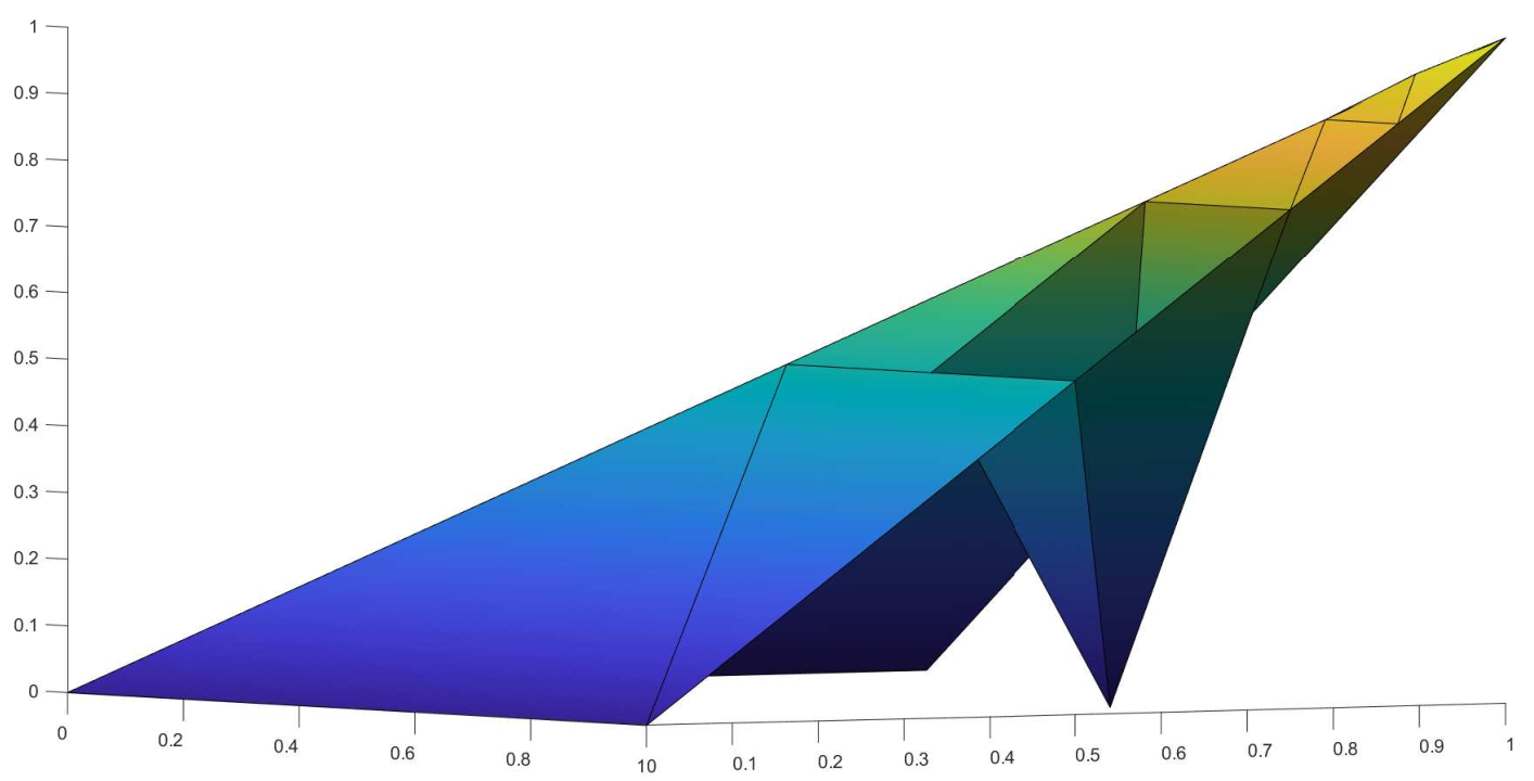
\begin{overpic}[mesh_VT0.pdf] \put(93.0,95.0){$\bm{x}$} \put(78.0,53.0){$\bm{x}^{*}$} \end{overpic}Refer to caption
Figure 2: Left: detail of a mesh 𝒯\mathcal{T}, in which red nodes 𝒙\bm{x} and 𝒙∗\bm{x^{*}} are proper nodes. Right: basis function ψ𝒙∈𝕍𝒯0\psi_{\bm{x}}\in\mathbb{V}_{\mathcal{T}}^{0}; notice that ψ𝒙​(𝒙∗)=0\psi_{\bm{x}}(\bm{x}^{*})=0 and the basis function ψ𝒙∗∈𝕍𝒯0\psi_{\bm{x}^{*}}\in\mathbb{V}_{\mathcal{T}}^{0} is the usual hat function supported in the square centered at 𝒙∗\bm{x}^{*} (not depicted).

Thus, it is natural to introduce the operator

ℐ𝒯0:𝕍𝒯→𝕍𝒯0\mathcal{I}_{\mathcal{T}}^{0}:\mathbb{V}_{\mathcal{T}}\to\mathbb{V}_{\mathcal{T}}^{0}

defined as the Lagrange interpolation operator at the nodes in 𝒫{\cal P}. The following result will be crucial in the forthcoming analysis.

Proposition 3.2 (comparison between interpolation operators).

Let 𝒯\mathcal{T} be Λ\Lambda-admissible. Then, there exists a constant CI>0C_{I}>0, depending on Λ\Lambda but independent of 𝒯\mathcal{T}, such that

|v−ℐ𝒯0​v|1,Ω≤CI​|v−ℐ𝒯​v|1,𝒯∀v∈𝕍𝒯.|v-\mathcal{I}_{\mathcal{T}}^{0}v|_{1,\Omega}\,\leq C_{I}\,|v-\mathcal{I}_{\mathcal{T}}v|_{1,\mathcal{T}}\qquad\forall v\in\mathbb{V}_{\mathcal{T}}\,. (3.3)

Note that the result is non-trivial, since the ‘non-conforming’ ℐ𝒯\mathcal{I}_{\mathcal{T}} may operate at a finer scale than the ‘conforming’ ℐ𝒯0\mathcal{I}_{\mathcal{T}}^{0}, although not too fine due to the condition of Λ\Lambda-admissibility. The proof of the result is postponed to Sect. 7.

We will also need some Clément quasi-interpolation operators. Precisely, let us denote by ℐ~𝒯0:𝕍→𝕍𝒯0\widetilde{\mathcal{I}}_{\mathcal{T}}^{0}:\mathbb{V}\to\mathbb{V}_{\mathcal{T}}^{0} the classical Clément operator on the finite-element space 𝕍𝒯0\mathbb{V}_{\mathcal{T}}^{0}; that is, the value at each internal (proper) node is the average of the target function on the support of the associated basis function. Similarly, let ℐ~𝒯:𝕍→𝕍𝒯\widetilde{\mathcal{I}}_{\mathcal{T}}:\mathbb{V}\to\mathbb{V}_{\mathcal{T}} be the Clément operator on the virtual-element space 𝕍𝒯\mathbb{V}_{\mathcal{T}}, as defined in [39].

Lemma 3.3 (Clement interpolation estimate).

The following inequality holds

∑E∈𝒯hE−2​‖v−ℐ~𝒯0​v‖0,E2≲|v|1,Ω2∀v∈𝕍,\sum_{E\in\mathcal{T}}h_{E}^{-2}\|v-\widetilde{\mathcal{I}}_{\mathcal{T}}^{0}v\|_{0,E}^{2}\lesssim|v|_{1,\Omega}^{2}\qquad\forall v\in\mathbb{V}\,, (3.4)

where the hidden constant depends on the maximal index Λ\Lambda but not on 𝒯\mathcal{T}.

Proof.

Let v𝒯=ℐ~𝒯​v∈𝕍𝒯v_{\mathcal{T}}=\widetilde{\mathcal{I}}_{\mathcal{T}}v\in\mathbb{V}_{\mathcal{T}}. Since v−ℐ~𝒯0​v=(v−v𝒯)+(v𝒯−ℐ~𝒯0​v𝒯)+(ℐ~𝒯0​v𝒯−ℐ~𝒯0​v)v-\widetilde{\mathcal{I}}_{\mathcal{T}}^{0}v=(v-v_{\mathcal{T}})+(v_{\mathcal{T}}-\widetilde{\mathcal{I}}_{\mathcal{T}}^{0}v_{\mathcal{T}})+(\widetilde{\mathcal{I}}_{\mathcal{T}}^{0}v_{\mathcal{T}}-\widetilde{\mathcal{I}}_{\mathcal{T}}^{0}v) and ℐ~𝒯0\widetilde{\mathcal{I}}_{\mathcal{T}}^{0} is locally stable in L2L^{2}, we deduce

∑E∈𝒯hE−2​‖v−ℐ~𝒯0​v‖0,E2\displaystyle\sum_{E\in\mathcal{T}}\!\!h_{E}^{-2}\|v-\widetilde{\mathcal{I}}_{\mathcal{T}}^{0}v\|_{0,E}^{2} ≲\displaystyle\lesssim ∑E∈𝒯hE−2​‖v−v𝒯‖0,E2+hE−2​‖v𝒯−ℐ~𝒯0​v𝒯‖0,E2≲|v|1,Ω2+∑E∈𝒯hE−2​‖v𝒯−ℐ~𝒯0​v𝒯‖0,E2.\displaystyle\sum_{E\in\mathcal{T}}\!\!h_{E}^{-2}\|v-v_{\mathcal{T}}\|_{0,E}^{2}+h_{E}^{-2}\|v_{\mathcal{T}}-\widetilde{\mathcal{I}}_{\mathcal{T}}^{0}v_{\mathcal{T}}\|_{0,E}^{2}\lesssim|v|_{1,\Omega}^{2}+\!\sum_{E\in\mathcal{T}}\!\!h_{E}^{-2}\|v_{\mathcal{T}}-\widetilde{\mathcal{I}}_{\mathcal{T}}^{0}v_{\mathcal{T}}\|_{0,E}^{2}.

Thus, we need to prove

∑E∈𝒯hE−2​‖v𝒯−ℐ~𝒯0​v𝒯‖0,E2≲|v𝒯|1,Ω2.\sum_{E\in\mathcal{T}}h_{E}^{-2}\|v_{\mathcal{T}}-\widetilde{\mathcal{I}}_{\mathcal{T}}^{0}v_{\mathcal{T}}\|_{0,E}^{2}\lesssim|v_{\mathcal{T}}|_{1,\Omega}^{2}.

To show this bound, write v𝒯−ℐ~𝒯0​v𝒯=(v𝒯−ℐ𝒯0​v𝒯)+ℐ~𝒯0​(ℐ𝒯0​v𝒯−v𝒯)v_{\mathcal{T}}-\widetilde{\mathcal{I}}_{\mathcal{T}}^{0}v_{\mathcal{T}}=(v_{\mathcal{T}}-{\mathcal{I}}_{\mathcal{T}}^{0}v_{\mathcal{T}})+\widetilde{\mathcal{I}}_{\mathcal{T}}^{0}({\mathcal{I}}_{\mathcal{T}}^{0}v_{\mathcal{T}}-v_{\mathcal{T}}) because ℐ~𝒯0\widetilde{\mathcal{I}}_{\mathcal{T}}^{0} is invariant in 𝕍𝒯0\mathbb{V}_{\mathcal{T}}^{0}, i.e. ℐ𝒯0​v𝒯=ℐ~𝒯0​(ℐ𝒯0​v𝒯){\mathcal{I}}_{\mathcal{T}}^{0}v_{\mathcal{T}}=\widetilde{\mathcal{I}}_{\mathcal{T}}^{0}({\mathcal{I}}_{\mathcal{T}}^{0}v_{\mathcal{T}}). We finally use again the stability of ℐ~𝒯0\widetilde{\mathcal{I}}_{\mathcal{T}}^{0} in L2L^{2} together with Proposition 3.1 to obtain

∑E∈𝒯hE−2​‖v𝒯−ℐ~𝒯0​v𝒯‖0,E2≲∑E∈𝒯hE−2​‖v𝒯−ℐ𝒯0​v𝒯‖0,E2≲CΛ​|v𝒯|1,Ω2.\sum_{E\in\mathcal{T}}h_{E}^{-2}\|v_{\mathcal{T}}-\widetilde{\mathcal{I}}_{\mathcal{T}}^{0}v_{\mathcal{T}}\|_{0,E}^{2}\lesssim\sum_{E\in\mathcal{T}}h_{E}^{-2}\|v_{\mathcal{T}}-{\mathcal{I}}_{\mathcal{T}}^{0}v_{\mathcal{T}}\|_{0,E}^{2}\lesssim C_{\Lambda}|v_{\mathcal{T}}|_{1,\Omega}^{2}.

This concludes the proof. ∎

4 A posteriori error analysis

Since we are interested in building adaptive discretizations, we rely on a posteriori error control. Following [25], we first introduce a residual-type a posteriori estimator. To this end, recalling that 𝒟=(A,c,f)\mathcal{D}=(A,c,f) denotes the set of piecewise constant data, for any v∈𝕍𝒯v\in\mathbb{V}_{\mathcal{T}} and any element EE let us define the internal residual over EE

r𝒯​(E,v,𝒟):=fE−cE​ΠE∇​v.r_{\mathcal{T}}(E;v,\mathcal{D}):=f_{E}\,-\,c_{E}\,{\Pi^{\nabla}_{E}}v\,. (4.1)

Similarly, for any two elements E1,E2∈𝒯E_{1},E_{2}\in\mathcal{T} sharing an edge e∈ℰE1∩ℰE2e\in\mathcal{E}_{E_{1}}\cap\mathcal{E}_{E_{2}}, let us define the jump residual over ee

j𝒯(e;v,𝒟):=[[A∇Π𝒯∇v]]e=(AE1∇ΠE1∇v|E1)⋅𝒏1+(AE2∇ΠE2∇v|E2)⋅𝒏2,j_{\mathcal{T}}(e;v,\mathcal{D}):=[\![\,A\nabla\,\Pi^{\nabla}_{\mathcal{T}}v\,]\!]_{e}=(A_{E_{1}}\nabla\,\Pi^{\nabla}_{E_{1}}v_{|E_{1}})\cdot\bm{n}_{1}+(A_{E_{2}}\nabla\,\Pi^{\nabla}_{E_{2}}v_{|E_{2}})\cdot\bm{n}_{2}\,, (4.2)

where 𝒏i\bm{n}_{i} denotes the unit normal vector to ee pointing outward with respect to EiE_{i}; set j𝒯​(e,v)=0j_{\mathcal{T}}(e;v)=0 if e⊂∂Ωe\subset\partial\Omega. Then, taking into account Remark 2.3, we define the local residual estimator associated with EE

η𝒯2​(E,v,𝒟):=hE2​‖r𝒯​(E,v,𝒟)‖0,E2+12​∑e∈ℰEhE​‖j𝒯​(e,v,𝒟)‖0,e2,\eta_{\mathcal{T}}^{2}(E;v,\mathcal{D}):=h_{E}^{2}\|r_{\mathcal{T}}(E;v,\mathcal{D})\|_{0,E}^{2}\ +\ \tfrac{1}{2}\sum_{e\in{\mathcal{E}_{E}}}h_{E}\|j_{\mathcal{T}}(e;v,\mathcal{D})\|_{0,e}^{2}\;, (4.3)

as well as the global residual estimator

η𝒯2​(v,𝒟):=∑E∈𝒯η𝒯2​(E,v,𝒟).\eta_{\mathcal{T}}^{2}(v,\mathcal{D}):=\sum_{E\in\mathcal{T}}\eta_{\mathcal{T}}^{2}(E;v,\mathcal{D})\,. (4.4)

An upper bound of the energy error is provided by the following result. The proof follows [25, Theorem 13], with the remarkable technical difference that the stabilization term S𝒯​(u𝒯,u𝒯)S_{\mathcal{T}}(u_{\mathcal{T}},u_{\mathcal{T}}) is not scaled by the constant γ\gamma in (4.5).

Proposition 4.1 (upper bound).

There exists a constant Capost>0C_{\text{apost}}>0 depending on Λ\Lambda and 𝒟\mathcal{D} but independent of uu, 𝒯\mathcal{T}, u𝒯u_{\mathcal{T}} and γ\gamma, such that

|u−u𝒯|1,Ω2≤Capost​(η𝒯2​(u𝒯,𝒟)+S𝒯​(u𝒯,u𝒯)).|u-u_{\mathcal{T}}|_{1,\Omega}^{2}\leq C_{\text{apost}}\left(\eta_{\mathcal{T}}^{2}(u_{\mathcal{T}},\mathcal{D})+S_{\mathcal{T}}(u_{\mathcal{T}},u_{\mathcal{T}})\right)\,. (4.5)
Proof.

We let v∈H01​(Ω)v\in H^{1}_{0}(\Omega) and proceed as in [25, Theorem 13] to write

ℬ⁡(u−u𝒯,v)=((f,v−v𝒯)Ω−ℬ⁡(u𝒯,v−v𝒯))+ℬ⁡(u−u𝒯,v𝒯)=:I+I​I,{\mathcal{B}}(u-u_{\mathcal{T}},v)=\big((f,v-v_{\mathcal{T}})_{\Omega}-{\mathcal{B}}(u_{\mathcal{T}},v-v_{\mathcal{T}})\big)+{\mathcal{B}}(u-u_{\mathcal{T}},v_{\mathcal{T}})=:I+II,

except that we choose v𝒯=ℐ~𝒯0​v∈𝕍𝒯0v_{\mathcal{T}}=\widetilde{\mathcal{I}}_{\mathcal{T}}^{0}v\in\mathbb{V}_{\mathcal{T}}^{0}, where ℐ~𝒯0\widetilde{\mathcal{I}}_{\mathcal{T}}^{0} is the Clément quasi-interpolation operator on 𝕍𝒯0\mathbb{V}_{\mathcal{T}}^{0}. This choice has a remarkable impact on (4.5) compared with [25, Theorem 13].

We start by estimating the term II: one has

I\displaystyle I =∑E∈𝒯{(f,v−v𝒯)E−(AE∇ΠE∇u𝒯,∇(v−v𝒯))E−cE(ΠE∇u𝒯,v−v𝒯)E}\displaystyle=\sum_{E\in\mathcal{T}}\left\{(f,v-v_{\mathcal{T}})_{E}-(A_{E}\nabla\Pi^{\nabla}_{E}u_{\mathcal{T}},\nabla(v-v_{\mathcal{T}}))_{E}-c_{E}(\Pi^{\nabla}_{E}u_{\mathcal{T}},v-v_{\mathcal{T}})_{E}\right\}
+∑E∈𝒯{(AE∇(ΠE∇u𝒯−u𝒯),∇(v−v𝒯))E+cE((ΠE∇u𝒯−u𝒯),v−v𝒯)E}=:I1+I2.\displaystyle+\sum_{E\in\mathcal{T}}\left\{(A_{E}\nabla(\Pi^{\nabla}_{E}u_{\mathcal{T}}-u_{\mathcal{T}}),\nabla(v-v_{\mathcal{T}}))_{E}+c_{E}((\Pi^{\nabla}_{E}u_{\mathcal{T}}-u_{\mathcal{T}}),v-v_{\mathcal{T}})_{E}\right\}=:I_{1}+I_{2}.

Integrating by parts, employing Lemma 3.3 and proceeding as in [25], we get

|I1|\displaystyle|I_{1}| ≲η𝒯​(u𝒯,𝒟)​|v|1,Ω\displaystyle\lesssim\eta_{\mathcal{T}}(u_{\mathcal{T}},\mathcal{D})|v|_{1,\Omega} (4.6)
|I2|\displaystyle|I_{2}| ≲(∑E∈𝒯‖∇(ΠE∇​u𝒯−u𝒯)‖0,E2+hE​‖ΠE∇​u𝒯−u𝒯‖0,E2)1/2​|v|1,Ω≲S𝒯​(u𝒯,u𝒯)1/2​|v|1,Ω.\displaystyle\lesssim\left(\sum_{E\in\mathcal{T}}\|\nabla(\Pi^{\nabla}_{E}u_{\mathcal{T}}-u_{\mathcal{T}})\|^{2}_{0,E}+h_{E}\|\Pi^{\nabla}_{E}u_{\mathcal{T}}-u_{\mathcal{T}}\|^{2}_{0,E}\right)^{1/2}|v|_{1,\Omega}\lesssim S_{\mathcal{T}}(u_{\mathcal{T}},u_{\mathcal{T}})^{1/2}|v|_{1,\Omega}\,. (4.7)

We now deal with term I​III. We first apply Lemma 2.6 to obtain

ℬ⁡(u−u𝒯,v𝒯)=∑E∈𝒯cE​∫E(ΠE∇​u𝒯−u𝒯)​v𝒯,{\mathcal{B}}(u-u_{\mathcal{T}},v_{\mathcal{T}})=\sum_{E\in\mathcal{T}}c_{E}\int_{E}(\Pi^{\nabla}_{E}u_{\mathcal{T}}-u_{\mathcal{T}})v_{\mathcal{T}},

because v𝒯∈𝕍𝒯0v_{\mathcal{T}}\in\mathbb{V}_{\mathcal{T}}^{0}; this is the key difference with [25, Theorem 13]. We next recall the definition (2.8) of ΠE∇\Pi^{\nabla}_{E}, and corresponding scaled Poincaré inequality ‖ΠE∇​u𝒯−u𝒯‖0,E≲hE​|ΠE∇​u𝒯−u𝒯|1,E\|\Pi^{\nabla}_{E}u_{\mathcal{T}}-u_{\mathcal{T}}\|_{0,E}\lesssim h_{E}\,|\Pi^{\nabla}_{E}u_{\mathcal{T}}-u_{\mathcal{T}}|_{1,E} for all E∈𝒯E\in\mathcal{T}, to arrive at

ℬ⁡(u−u𝒯,v𝒯)≲hE​S𝒯​(u𝒯,u𝒯)1/2​|v𝒯|1,Ω.{\mathcal{B}}(u-u_{\mathcal{T}},v_{\mathcal{T}})\lesssim h_{E}\,S_{\mathcal{T}}(u_{\mathcal{T}},u_{\mathcal{T}})^{1/2}|v_{\mathcal{T}}|_{1,\Omega}.

Finally, taking v=u−u𝒯∈H01​(Ω)v=u-u_{\mathcal{T}}\in H^{1}_{0}(\Omega), employing the coercivity of ℬ⁡(⋅,⋅){\mathcal{B}}(\cdot,\cdot) and combining the above estimates yield the assertion. ∎

We state the following result, which is proven in [25] for the choice (2.7) but it holds with the same proof for any other admissible choice of 𝕍E{\mathbb{V}_{E}}.

Proposition 4.2 (local lower bound).

There holds

η𝒯2​(E,u𝒯,𝒟)≲∑E′∈ωE(|u−u𝒯|1,E′2+SE′​(u𝒯,u𝒯))\eta_{\mathcal{T}}^{2}(E;u_{\mathcal{T}},\mathcal{D})\lesssim\sum_{E^{\prime}\in\omega_{E}}\left(|u-u_{\mathcal{T}}|^{2}_{1,E^{\prime}}+S_{E^{\prime}}(u_{\mathcal{T}},u_{\mathcal{T}})\right) (4.8)

where ωE:={E′:|∂E∩∂E′|≠0}\omega_{E}:=\{E^{\prime}:|\partial E\cap\partial E^{\prime}|\not=0\}. The hidden constant is independent of γ,h,u\gamma,h,u and u𝒯u_{\mathcal{T}}.

Corollary 4.3 (global lower bound).

There exists a constant capost>0c_{\text{apost}}>0, depending on Λ\Lambda but independent of uu, 𝒯\mathcal{T}, u𝒯u_{\mathcal{T}} and γ\gamma, such that

capost​η𝒯2​(u𝒯,𝒟)≤|u−u𝒯|1,Ω2+S𝒯​(u𝒯,u𝒯).c_{\text{apost}}\,\eta_{\mathcal{T}}^{2}(u_{\mathcal{T}},\mathcal{D})\leq|u-u_{\mathcal{T}}|^{2}_{1,\Omega}+S_{\mathcal{T}}(u_{\mathcal{T}},u_{\mathcal{T}})\,. (4.9)

We now state one of the two main results contained in this paper. Due to the technical nature of the proof, we postpone it to Sect. 8.

Proposition 4.4 (bound of the stabilization term by the residual).

There exists a constant CB>0C_{B}>0 depending on Λ\Lambda but independent of 𝒯\mathcal{T}, u𝒯u_{\mathcal{T}} and γ\gamma such that

γ2​S𝒯​(u𝒯,u𝒯)≤CB​η𝒯2​(u𝒯,𝒟).\gamma^{2}S_{\mathcal{T}}(u_{\mathcal{T}},u_{\mathcal{T}})\leq C_{B}\,\eta_{\mathcal{T}}^{2}(u_{\mathcal{T}},\mathcal{D})\,. (4.10)

Combining Proposition 4.1, Corollary 4.3 and Proposition 4.4, we get the following stabilization-free (global) upper and lower bounds.

Corollary 4.5 (stabilization-free a posteriori error estimates).

Assume that the parameter γ\gamma is chosen to satisfy γ2>CBcapost\gamma^{2}>\displaystyle{\frac{C_{B}}{c_{\text{apost}}}}. Then it holds

CL​η𝒯2​(u𝒯,𝒟)≤|u−u𝒯|1,Ω2≤CU​η𝒯2​(u𝒯,𝒟),C_{L}\eta_{\mathcal{T}}^{2}(u_{\mathcal{T}},\mathcal{D})\leq|u-u_{\mathcal{T}}|_{1,\Omega}^{2}\leq C_{U}\eta_{\mathcal{T}}^{2}(u_{\mathcal{T}},\mathcal{D})\,, (4.11)

with CL=capost−CB​γ−2C_{L}=c_{\text{apost}}-C_{B}\gamma^{-2} and CU=Capost​(1+CB​γ−2)C_{U}=C_{\text{apost}}\,\left(1+C_{B}\gamma^{-2}\right).

The sharpness of (4.11) will be investigated also from the numerical standpoint in Section 10.2.

5 Adaptive VEM with contraction property

In Section 5.1, we introduce an Adaptive Virtual Element Method (AVEM), called GALERKIN, for approximating (2.2) to a given tolerance under Assumption 2.4 (piecewise constant data). We investigate the effect of local mesh refinements on our error estimator in Section 5.2, and prove a contraction property of GALERKIN in Section 5.3. The design and analysis of an AVEM able to handle also variable data is postponed to [15].

5.1 The module GALERKIN

Given a Λ\Lambda-admissible input mesh 𝒯0\mathcal{T}_{0}, piecewise constant input data 𝒟\mathcal{D} on 𝒯0\mathcal{T}_{0} and a tolerance ε>0\varepsilon>0, the call

[𝒯,u𝒯]=𝙶𝙰𝙻𝙴𝚁𝙺𝙸𝙽⁡(𝒯0,𝒟,ε)[\mathcal{T},u_{\mathcal{T}}]={\tt GALERKIN}(\mathcal{T}_{0},\mathcal{D},\varepsilon) (5.1)

produces a Λ\Lambda-admissible bisection refinement 𝒯\mathcal{T} of 𝒯0\mathcal{T}_{0} and the Galerkin approximation u𝒯∈𝕍𝒯u_{\mathcal{T}}\in\mathbb{V}_{\mathcal{T}} to the solution u{u} of problem (2.1) with piecewise constant data 𝒟\mathcal{D} on 𝒯0\mathcal{T}_{0}, such that

‖|u−u𝒯|‖≤CG​ε,|\!|\!|u-u_{\mathcal{T}}|\!|\!|\leq C_{G}\,\varepsilon\,, (5.2)

with CG=cℬ​CUC_{G}=\sqrt{c^{\mathcal{B}}C_{U}}, where cℬc^{\mathcal{B}} is defined in (2.3) and CUC_{U} is the upper bound constant in Corollary 4.5. This is obtained by iterating the classical paradigm

SOLVE⟶ESTIMATE⟶MARK⟶REFINE\texttt{SOLVE}\,\,\longrightarrow\,\,\texttt{ESTIMATE}\,\,\longrightarrow\,\,\texttt{MARK}\,\,\longrightarrow\,\,\texttt{REFINE} (5.3)

thereby producing a sequence of Λ\Lambda-admissible meshes {𝒯k}k≥0\{\mathcal{T}_{k}\}_{k\geq 0}, and associated Galerkin solutions uk∈𝕍𝒯ku_{k}\in\mathbb{V}_{\mathcal{T}_{k}} to the problem (2.1) with data 𝒟\mathcal{D}. The iteration stops as soon as η𝒯k​(uk,𝒟)≤ε\eta_{\mathcal{T}_{k}}(u_{k},\mathcal{D})\leq\varepsilon, which is possible thanks to the convergence result stated in Theorem 5.1 below.

The modules in (5.3) are defined as follows: given piecewise constant data 𝒟\mathcal{D} on 𝒯0\mathcal{T}_{0},

  1. ∙\bullet

    [u𝒯]=SOLVE​(𝒯,𝒟)[u_{\mathcal{T}}]=\texttt{SOLVE}(\mathcal{T},\mathcal{D}) produces the Galerkin solution on the mesh 𝒯\mathcal{T} for data 𝒟\mathcal{D};

  2. ∙\bullet

    [{η𝒯​(⋅,u𝒯,𝒟)}]=ESTIMATE​(𝒯,u𝒯)[\{\eta_{\mathcal{T}}(\,\cdot\,;u_{\mathcal{T}},\mathcal{D})\}]=\texttt{ESTIMATE}(\mathcal{T},u_{\mathcal{T}}) computes the local residual estimators (4.3) on the mesh 𝒯\mathcal{T}, which depend on the Galerkin solution u𝒯u_{\mathcal{T}} and data 𝒟\mathcal{D};

  3. ∙\bullet

    [ℳ]=MARK​(𝒯,{η𝒯​(⋅,u𝒯,𝒟)},θ)[\mathcal{M}]=\texttt{MARK}(\mathcal{T},\{\eta_{\mathcal{T}}(\,\cdot\,;u_{\mathcal{T}},\mathcal{D})\},\theta) implements the Dörfler criterion [33], namely for a given parameter θ∈(0,1)\theta\in(0,1) an almost minimal set ℳ⊂𝒯\mathcal{M}\subset\mathcal{T} is found such that

    θ​η𝒯2​(u𝒯,𝒟)≤∑E∈ℳη𝒯2​(E,u𝒯,𝒟);\theta\eta_{\mathcal{T}}^{2}(u_{\mathcal{T}},\mathcal{D})\leq\sum_{E\in\mathcal{M}}\eta_{\mathcal{T}}^{2}(E;u_{\mathcal{T}},\mathcal{D})\,; (5.4)
  4. ∙\bullet

    [𝒯∗]=REFINE​(𝒯,ℳ,Λ)[{\mathcal{T}_{*}}]=\texttt{REFINE}(\mathcal{T},\mathcal{M},\Lambda) produces a Λ\Lambda-admissible refinement 𝒯∗{\mathcal{T}_{*}} of 𝒯\mathcal{T}, obtained by newest-vertex bisection of all the elements in ℳ\mathcal{M} and, possibly, some other elements of 𝒯\mathcal{T}.

In the procedure REFINE, non-admissible hanging nodes, i.e., hanging nodes with global index larger than Λ\Lambda, might be created while refining elements in ℳ\mathcal{M}. Thus, in order to obtain a Λ\Lambda-admissible partition 𝒯∗{\mathcal{T}_{*}}, REFINE possibly refines other elements in 𝒯\mathcal{T} (completion). A practical completion procedure, called MAKE_ADMISSIBLE, is described in Section 10.1, while the complexity analysis of such a procedure is discussed in the forthcoming paper [15].

The following crucial property of GALERKIN guarantees its convergence in a finite number of iterations proportional to |log⁡ε||\log\varepsilon|. We postpone its proof to Section 5.3.

Theorem 5.1 (contraction property of GALERKIN).

Let ℳ⊂𝒯\mathcal{M}\subset\mathcal{T} be the set of marked elements relative to the Galerkin solution u𝒯∈𝕍𝒯u_{\mathcal{T}}\in\mathbb{V}_{\mathcal{T}}. If 𝒯∗{\mathcal{T}_{*}} is the refinement of 𝒯\mathcal{T} obtained by applying REFINE, then for γ\gamma sufficiently large, there exist constants α∈(0,1)\alpha\in(0,1) and β>0\beta>0 such that one has

‖|u−u𝒯∗|‖2+β​η𝒯∗2​(u𝒯∗,𝒟)≤α⁡(‖|u−u𝒯|‖2+β​η𝒯2​(u𝒯,𝒟)).\displaystyle|\!|\!|u-u_{\mathcal{T}_{*}}|\!|\!|^{2}+\beta\eta_{\mathcal{T}_{*}}^{2}(u_{\mathcal{T}_{*}},\mathcal{D})\leq\alpha\left(|\!|\!|u-u_{\mathcal{T}}|\!|\!|^{2}+\beta\eta_{\mathcal{T}}^{2}(u_{\mathcal{T}},\mathcal{D})\right). (5.5)

5.2 Error estimator under local mesh refinements

In this section we prove three crucial properties of the error estimator that will be employed in studying the convergence of GALERKIN.

Let 𝒯∗{\mathcal{T}_{*}} be a refinement of 𝒯\mathcal{T} produced by REFINE by bisection. Consider an element E∈𝒯E\in\mathcal{T} which has been split into two elements E1,E2∈𝒯∗E_{1},E_{2}\in{\mathcal{T}_{*}}. If v∈𝕍𝒯v\in\mathbb{V}_{\mathcal{T}}, then vv is known on ∂E\partial E, hence in particular at the new vertex of E1,E2E_{1},E_{2} created by bisection. Thus, vv is known at all nodes (vertices and possibly hanging nodes) sitting on ∂E1\partial E_{1} and ∂E2\partial E_{2}, since the new edge e=E1∩E2e=E_{1}\cap E_{2} does not contain internal nodes. This uniquely identifies a function in 𝕍E1\mathbb{V}_{E_{1}} and a function in 𝕍E2\mathbb{V}_{E_{2}}, which are continuous across ee. In this manner, we associate to any v∈𝕍𝒯v\in\mathbb{V}_{\mathcal{T}} a unique function v∗∈𝕍𝒯∗v_{*}\in\mathbb{V}_{\mathcal{T}_{*}}, that coincides with vv on the skeleton ℰ\mathcal{E} (but possibly not on ℰ∗{\mathcal{E}_{*}}). We will actually write vv for v∗v_{*} whenever no confusion is possible.

a. Comparison of residuals under refinement

Let 𝒯∗{\mathcal{T}_{*}} be a refinement of 𝒯\mathcal{T} as above, and let E∈𝒯E\in\mathcal{T} be an element that has been split into two elements E1,E2∈𝒯∗E_{1},E_{2}\in{\mathcal{T}_{*}}; observe that hEi=12​hEh_{E_{i}}=\frac{1}{\sqrt{2}}h_{E}, i=1,2i=1,2. Given v∈𝕍𝒯v\in\mathbb{V}_{\mathcal{T}}, we aim at comparing the local residual estimator η𝒯​(E,v,𝒟)\eta_{\mathcal{T}}(E;v,\mathcal{D}) defined in (4.3) to the local estimator η𝒯∗​(E,v,𝒟)\eta_{\mathcal{T}_{*}}(E;v,\mathcal{D}) defined by

η𝒯∗2​(E,v,𝒟):=∑i=12η𝒯∗2​(Ei,v,𝒟)=∑i=12hEi2​‖fEi−cEi​ΠEi∇​v‖0,Ei2+12​∑i=12∑e∈ℰEihEi​‖j𝒯∗​(e,v)‖0,e2\eta_{\mathcal{T}_{*}}^{2}(E;v,\mathcal{D}):=\sum_{i=1}^{2}\eta_{\mathcal{T}_{*}}^{2}(E_{i};v,\mathcal{D})=\sum_{i=1}^{2}h_{E_{i}}^{2}\|f_{E_{i}}\,-\,c_{E_{i}}\,{\Pi^{\nabla}_{E_{i}}}v\|_{0,E_{i}}^{2}+\tfrac{1}{2}{\sum_{i=1}^{2}\sum_{e\in{\cal E}_{E_{i}}}h_{E_{i}}\|j_{{\mathcal{T}_{*}}}(e;v)\|_{0,e}^{2}}\; (5.6)

where it is important to observe that, as 𝒟\mathcal{D} does not change under refinement, we have fEi=fE|Eif_{E_{i}}=f_{E}|_{E_{i}}, cEi=cE|Eic_{E_{i}}=c_{E}|_{E_{i}}, AEi=AE|EiA_{E_{i}}=A_{E}|_{E_{i}}.

Lemma 5.2 (local estimator reduction).

There exist constants μ∈(0,1)\mu\in(0,1) and ce​r,1>0{c_{er,1}}>0 independent of 𝒯\mathcal{T} such that for any element E∈𝒯E\in\mathcal{T} which is split into two children E1,E2∈𝒯∗E_{1},E_{2}\in{\mathcal{T}_{*}}, one has

η𝒯∗​(E,v,𝒟)≤μ​η𝒯​(E,v,𝒟)+ce​r,1​S𝒯⁡(E)1/2​(v,v)∀v∈𝕍𝒯,\eta_{\mathcal{T}_{*}}(E;v,\mathcal{D})\leq\mu\ \eta_{\mathcal{T}}(E;v,\mathcal{D})+{c_{er,1}}\,S^{1/2}_{\mathcal{T}(E)}(v,v)\qquad\forall v\in\mathbb{V}_{\mathcal{T}}\,, (5.7)

where S𝒯⁡(E)​(v,v):=∑E′∈𝒯⁡(E)SE′​(v,v)S_{\mathcal{T}(E)}(v,v):=\sum_{E^{\prime}\in\mathcal{T}(E)}S_{E^{\prime}}(v,v) with 𝒯⁡(E):={E′∈𝒯:ℰE∩ℰE′≠∅}\mathcal{T}(E):=\{E^{\prime}\in\mathcal{T}:{\cal E}_{E}\cap{\cal E}_{E^{\prime}}\not=\emptyset\}.

Proof.

As fEf_{E} and cEc_{E} do not change under refinement, we simplify the notation and write rE=f−c​ΠE∇​vr_{E}=f-c{\Pi^{\nabla}_{E}}v, rEi=f−c​ΠEi∇​vr_{E_{i}}=f-c{\Pi^{\nabla}_{E_{i}}}v (i=1,2) with f=fEf=f_{E} and c=cEc=c_{E}. We have rEi=f−c​ΠEi∇​v=rE+c⁡(ΠE∇​v−ΠEi∇​v)r_{E_{i}}=f-c{\Pi^{\nabla}_{E_{i}}}v=r_{E}+c({\Pi^{\nabla}_{E}}v-{\Pi^{\nabla}_{E_{i}}}v), whence

∑i=12hEi2​‖rEi‖0,Ei2\displaystyle\sum_{i=1}^{2}h_{E_{i}}^{2}\|r_{E_{i}}\|_{0,E_{i}}^{2} ≤∑i=12hEi2​((1+ϵ)​‖rE‖0,Ei2+(1+1ϵ)​‖c⁡(ΠE∇​v−ΠEi∇​v)‖0,Ei2)\displaystyle\leq\sum_{i=1}^{2}h_{E_{i}}^{2}\left((1+\epsilon)\|r_{E}\|_{0,E_{i}}^{2}+\left(1+\frac{1}{\epsilon}\right)\|c({\Pi^{\nabla}_{E}}v-{\Pi^{\nabla}_{E_{i}}}v)\|_{0,E_{i}}^{2}\right) (5.8)
≤1+ϵ2​hE2​‖rE‖0,E2+hE2​(1+1ϵ)​cE22​∑i=12‖ΠE∇​v−ΠEi∇​v‖0,Ei2.\displaystyle\leq\frac{1+\epsilon}{2}h_{E}^{2}\|r_{E}\|_{0,E}^{2}+h_{E}^{2}\left(1+\frac{1}{\epsilon}\right)\frac{{c_{E}^{2}}}{2}\sum_{i=1}^{2}\|{\Pi^{\nabla}_{E}}v-{\Pi^{\nabla}_{E_{i}}}v\|_{0,E_{i}}^{2}.

In addition, we see that ∑i=12‖ΠE∇​v−ΠEi∇​v‖0,Ei2≤2​‖v−ΠE∇​v‖0,E2+2​∑i=12‖v−ΠEi∇​v‖0,Ei2.\displaystyle{\sum_{i=1}^{2}\|{\Pi^{\nabla}_{E}}v-{\Pi^{\nabla}_{E_{i}}}v\|_{0,E_{i}}^{2}\leq 2\|v-{\Pi^{\nabla}_{E}}v\|_{0,E}^{2}+2\sum_{i=1}^{2}\|v-{\Pi^{\nabla}_{E_{i}}}v\|_{0,E_{i}}^{2}}. Applying the Poincaré inequality and the minimality of ΠE∇{\Pi^{\nabla}_{E}}, we get

‖v−ΠE∇​v‖0,E2\displaystyle\|v-{\Pi^{\nabla}_{E}}v\|_{0,E}^{2} ≲|ΠE∇​v−v|1,E2≤|ℐE​v−v|1,E2,\displaystyle\lesssim|{\Pi^{\nabla}_{E}}v-v|_{1,E}^{2}\leq|\mathcal{I}_{E}v-v|_{1,E}^{2}\,,
∑i=12‖v−ΠEi∇​v‖0,Ei2\displaystyle\sum_{i=1}^{2}\|v-{\Pi^{\nabla}_{E_{i}}}v\|_{0,E_{i}}^{2} ≲∑i=12|v−ΠEi∇​v|1,Ei2≲|v−ΠE∇​v|1,E2≤|v−ℐE​v|1,E2.\displaystyle\lesssim\sum_{i=1}^{2}|v-{\Pi^{\nabla}_{E_{i}}}v|_{1,E_{i}}^{2}\lesssim|v-{\Pi^{\nabla}_{E}}v|_{1,E}^{2}\leq|v-\mathcal{I}_{E}v|_{1,E}^{2}.

Therefore, choosing ϵ=12\epsilon=\frac{1}{2}, setting μ:=1+ϵ2=34\mu:=\frac{1+\epsilon}{2}=\frac{3}{4} in (5.8), and employing (2.18) we infer that

∑i=12hEi2​‖rEi‖0,Ei2≤μ​hE2​‖rE‖0,E2+C​hE2​|v−ℐE​v|1,E2≤μ​hE2​‖rE‖0,E2+C​hE2​SE​(v,v).\displaystyle\sum_{i=1}^{2}h_{E_{i}}^{2}\|r_{E_{i}}\|_{0,E_{i}}^{2}\leq\mu\,h_{E}^{2}\|r_{E}\|_{0,E}^{2}+Ch_{E}^{2}|v-\mathcal{I}_{E}v|_{1,E}^{2}\leq\mu\,h_{E}^{2}\|r_{E}\|_{0,E}^{2}+Ch_{E}^{2}S_{E}(v,v). (5.9)

Concerning the jump terms, we first observe that writing j𝒯∗​(e,v)=j𝒯​(e,v)+(j𝒯∗​(e,v)−j𝒯​(e,v))j_{{\mathcal{T}_{*}}}(e;v)=j_{\mathcal{T}}(e;v)+\big(j_{{\mathcal{T}_{*}}}(e;v)-j_{\mathcal{T}}(e;v)\big), one has for any ϵ>0\epsilon>0

∑i=12∑e∈ℰEihEi​‖j𝒯∗​(e,v)‖0,e2≤(1+ϵ)​T1+(1+1ϵ)​T2,\sum_{i=1}^{2}\sum_{e\in{\cal E}_{E_{i}}}h_{E_{i}}\|j_{{\mathcal{T}_{*}}}(e;v)\|_{0,e}^{2}\leq(1+\epsilon)T_{1}+\left(1+\tfrac{1}{\epsilon}\right)T_{2}\,, (5.10)

with T1:=∑i=12∑e∈ℰEihEi​‖j𝒯​(e,v)‖0,e2T_{1}:=\displaystyle{\sum_{i=1}^{2}\sum_{e\in{\cal E}_{E_{i}}}h_{E_{i}}\|j_{\mathcal{T}}(e;v)\|_{0,e}^{2}}, T2:=∑i=12∑e∈ℰEihEi​‖j𝒯∗​(e,v)−j𝒯​(e,v)‖0,e2T_{2}:=\displaystyle{\sum_{i=1}^{2}\sum_{e\in{\cal E}_{E_{i}}}h_{E_{i}}\|j_{{\mathcal{T}_{*}}}(e;v)-j_{\mathcal{T}}(e;v)\|_{0,e}^{2}}.

Considering T1T_{1}, notice that j𝒯​(e,v)=0j_{\mathcal{T}}(e;v)=0 on the new edge created by the bisection of EE; hence,

T1≤12​∑e∈ℰEhE​‖j𝒯​(e,v)‖0,e2.T_{1}\leq\frac{1}{\sqrt{2}}\sum_{e\in{\cal E}_{E}}h_{E}\|j_{\mathcal{T}}(e;v)\|_{0,e}^{2}\,. (5.11)

In order to bound the second term T2T_{2}, define 𝒯∗​(Ei):={E′∈𝒯∗:ℰEi∩ℰE′≠∅}{\mathcal{T}_{*}}(E_{i}):=\{E^{\prime}\in{\mathcal{T}_{*}}:{\cal E}_{E_{i}}\cap{\cal E}_{E^{\prime}}\not=\emptyset\}; for an edge e∈ℰEie\in{\cal E}_{E_{i}}, let Ei,e∈𝒯∗​(Ei)E_{i,e}\in{\mathcal{T}_{*}}(E_{i}) be such that e=∂Ei∩∂Ei,ee=\partial E_{i}\cap\partial E_{i,e}. Then,

‖j𝒯∗​(e,v)−j𝒯​(e,v)‖0,e\displaystyle\|j_{{\mathcal{T}_{*}}}(e;v)-j_{\mathcal{T}}(e;v)\|_{0,e} =∥[[A∇(Π∇𝒯∗−Π∇𝒯)v]]∥0,e\displaystyle=\|[\![\,A\nabla(\Pi^{\nabla}_{\mathcal{T}_{*}}-\Pi^{\nabla}_{\mathcal{T}})v\,]\!]\|_{0,e}
≤∥AE∇(Π∇Ei−Π∇E)v∥0,e+∥AE^i,e∇(Π∇Ei,e−Π∇E^i,e)v∥0,e,\displaystyle\leq\|A_{E}\nabla(\Pi^{\nabla}_{E_{i}}-\Pi^{\nabla}_{E})v\|_{0,e}+\|A_{\widehat{E}_{i,e}}\nabla(\Pi^{\nabla}_{E_{i,e}}-\Pi^{\nabla}_{\hat{E}_{i,e}})v\|_{0,e}\,,

where, in general, F^∈𝒯\widehat{F}\in\mathcal{T} denotes the parent element of F∈𝒯∗F\in{\mathcal{T}_{*}}. Hence, using the trace inequality and the equivalence hEi≃hEi,eh_{E_{i}}\simeq h_{E_{i,e}}, we easily get

T2\displaystyle T_{2} ≲∑i=12∑E′∈𝒯∗​(Ei)∥∇(Π∇E′−Π∇E^′)v∥0,E′2≲∑i=12∑E′∈𝒯∗​(Ei)(∥∇(v−Π∇E′v)∥0,E′2+∥∇(v−Π∇E^′v)∥0,E′2).\displaystyle\lesssim\sum_{i=1}^{2}\sum_{E^{\prime}\in{\mathcal{T}_{*}}(E_{i})}\|\nabla(\Pi^{\nabla}_{E^{\prime}}-\Pi^{\nabla}_{\widehat{E}^{\prime}})v\|_{0,E^{\prime}}^{2}\lesssim\sum_{i=1}^{2}\sum_{E^{\prime}\in{\mathcal{T}_{*}}(E_{i})}\big(\|\nabla(v-\Pi^{\nabla}_{E^{\prime}}v)\|_{0,E^{\prime}}^{2}+\|\nabla(v-\Pi^{\nabla}_{\widehat{E}^{\prime}}v)\|_{0,E^{\prime}}^{2}\big)\,.

The minimality property of the orthogonal projections ΠE′∇\Pi^{\nabla}_{E^{\prime}} and ΠE^′∇\Pi^{\nabla}_{\widehat{E}^{\prime}} yields

‖∇(v−ΠE′∇​v)‖0,E′≤‖∇(v−ℐE^′​v)‖0,E′≤‖∇(v−ℐE^′​v)‖0,E^′\|\nabla(v-\Pi^{\nabla}_{E^{\prime}}v)\|_{0,E^{\prime}}\leq\|\nabla(v-{\cal I}_{\widehat{E}^{\prime}}v)\|_{0,E^{\prime}}\leq\|\nabla(v-{\cal I}_{\widehat{E}^{\prime}}v)\|_{0,\widehat{E}^{\prime}}

and

‖∇(v−ΠE^′∇​v)‖0,E′≤‖∇(v−ΠE^′∇​v)‖0,E^′≤‖∇(v−ℐE^′​v)‖0,E^′.\|\nabla(v-\Pi^{\nabla}_{\widehat{E}^{\prime}}v)\|_{0,E^{\prime}}\leq\|\nabla(v-\Pi^{\nabla}_{\widehat{E}^{\prime}}v)\|_{0,\widehat{E}^{\prime}}\leq\|\nabla(v-{\cal I}_{\widehat{E}^{\prime}}v)\|_{0,\widehat{E}^{\prime}}\,.

This gives

T2≤C​∑E′∈𝒯⁡(E)‖∇(v−ℐE′​v)‖0,E′2≤C​∑E′∈𝒯⁡(E)SE′​(v,v),T_{2}\leq C\sum_{E^{\prime}\in\mathcal{T}(E)}\|\nabla(v-{\cal I}_{{E}^{\prime}}v)\|_{0,{E}^{\prime}}^{2}\leq C\sum_{E^{\prime}\in\mathcal{T}(E)}S_{E^{\prime}}(v,v)\,, (5.12)

thanks to (2.15) and (2.16). Using (5.9), (5.10) with a sufficiently small ϵ\epsilon, (5.11) and (5.12), we arrive at the desired result. ∎

b. Lipschitz continuity of the residual estimator

Since the following result can be proven by standard arguments, we only sketch its proof.

Lemma 5.3 (Lipschitz continuity of error estimator).

There exists a constant ce​r,2>0{c_{er,2}}>0 independent of 𝒯\mathcal{T} such that for any element E∈𝒯E\in\mathcal{T}, one has

|η𝒯​(E,v,𝒟)−η𝒯​(E,w,𝒟)|≤ce​r,2​|v−w|1,𝒯⁡(E)∀v,w∈H1​(Ω),\big|\eta_{\mathcal{T}}(E;v,\mathcal{D})-\eta_{\mathcal{T}}(E;w,\mathcal{D})\big|\leq{c_{er,2}}\,|v-w|_{1,\mathcal{T}(E)}\qquad\forall v,w\in{H^{1}(\Omega)}\,, (5.13)

where |v−w|1,𝒯⁡(E)2:=∑E′∈𝒯⁡(E)|v−w|1,E′2|v-w|_{1,\mathcal{T}(E)}^{2}:=\sum_{E^{\prime}\in\mathcal{T}(E)}|v-w|_{1,E^{\prime}}^{2}.

Proof.

By standard FE arguments, using the fact that η𝒯​(E,v,𝒟)\eta_{\mathcal{T}}(E;v,\mathcal{D}) and η𝒯​(E,w,𝒟)\eta_{\mathcal{T}}(E;w,\mathcal{D}) are written in terms of ΠE∇​v{\Pi^{\nabla}_{E}}v and ΠE∇​w{\Pi^{\nabla}_{E}}w, which are polynomials, and employing inverse estimates, we easily obtain

|η𝒯​(E,v,𝒟)−η𝒯​(E,w,𝒟)|≤C​|Π𝒯⁡(E)∇​(v−w)|1,𝒯⁡(E)≤C​|v−w|1,𝒯⁡(E),\displaystyle\big|\eta_{\mathcal{T}}(E;v,\mathcal{D})-\eta_{\mathcal{T}}(E;w,\mathcal{D})\big|\leq C\,|\Pi^{\nabla}_{\mathcal{T}(E)}(v-w)|_{1,\mathcal{T}(E)}\leq C\,|v-w|_{1,\mathcal{T}(E)}\,, (5.14)

where the last inequality uses the definition of ΠE∇{\Pi^{\nabla}_{E}}. ∎

c. Reduction property for the local residual estimators

Concatenating Lemma 5.2 with Lemma 5.3 we arrive at the following reduction property for the local residual estimators.

Proposition 5.4 (estimator reduction property on refined elements).

There exist constants μ∈(0,1){\mu}\in(0,1), ce​r,1>0{c_{er,1}}>0 and ce​r,2>0{c_{er,2}}>0 independent of 𝒯\mathcal{T} such that for any v∈𝕍𝒯v\in\mathbb{V}_{\mathcal{T}} and w∈𝕍𝒯∗w\in\mathbb{V}_{\mathcal{T}_{*}}, and any element E∈𝒯E\in\mathcal{T} which is split into two children E1,E2∈𝒯∗E_{1},E_{2}\in{\mathcal{T}_{*}}, one has

η𝒯∗​(E,w,𝒟)≤μ​η𝒯​(E,v,𝒟)+ce​r,1​S𝒯⁡(E)1/2​(v,v)+ce​r,2​|v−w|1,𝒯⁡(E).\eta_{\mathcal{T}_{*}}(E;w,\mathcal{D})\leq{\mu}\ \eta_{\mathcal{T}}(E;v,\mathcal{D})+{c_{er,1}}\,S^{1/2}_{\mathcal{T}(E)}(v,v)+{c_{er,2}}\,|v-w|_{1,\mathcal{T}(E)}\,. (5.15)
Proof.

Employing Lemma 5.3 with 𝒯\mathcal{T} replaced by 𝒯∗{\mathcal{T}_{*}}, we get

η𝒯∗​(E,w,𝒟)≤η𝒯∗​(E,v,𝒟)+ce​r,2​|v−w|1,𝒯∗​(E).\eta_{\mathcal{T}_{*}}(E;w,\mathcal{D})\leq\eta_{\mathcal{T}_{*}}(E;v,\mathcal{D})+{c_{er,2}}\,|v-w|_{1,{\mathcal{T}_{*}}(E)}\,.

Finally, noting that 𝒯∗​(E){\mathcal{T}_{*}}(E) is a refinement of 𝒯⁡(E)\mathcal{T}(E), we conclude using Lemma 5.2. ∎

5.3 Convergence of AVEM

In this section we aim at proving Theorem 5.1 (contraction property of REFINE). To do so, since we first need to quantify the estimator and error reduction under refinement, we divide our argument into three steps.

a. Estimator reduction

We first study the effect of mesh refinement on the estimator.

Proposition 5.5 (estimator reduction).

Let ℳ⊂𝒯\mathcal{M}\subset\mathcal{T} be the set of marked elements in MARK, relative to the Galerkin solution u𝒯∈𝕍𝒯u_{\mathcal{T}}\in\mathbb{V}_{\mathcal{T}}, and let 𝒯∗{\mathcal{T}_{*}} be the refinement produced by REFINE. Then, there exist constants ρ<1\rho<1 and Ce​r,1,Ce​r,2>0C_{er,1},C_{er,2}>0 independent of 𝒯\mathcal{T} such that for all w∈𝕍𝒯∗w\in\mathbb{V}_{\mathcal{T}_{*}} one has

η𝒯∗2​(𝒯∗,w,𝒟)≤ρ​η𝒯2​(𝒯,u𝒯,𝒟)+Ce​r,1​S𝒯​(u𝒯,u𝒯)+Ce​r,2​|u𝒯−w|1,Ω2.\eta_{\mathcal{T}_{*}}^{2}({\mathcal{T}_{*}};w,\mathcal{D})\leq\rho\ \eta_{\mathcal{T}}^{2}(\mathcal{T};u_{\mathcal{T}},\mathcal{D})+C_{er,1}\,S_{\mathcal{T}}(u_{\mathcal{T}},u_{\mathcal{T}})+C_{er,2}\,|u_{\mathcal{T}}-w|^{2}_{1,\Omega}\,. (5.16)
Proof.

For simplicity of notation, let us set v=u𝒯v=u_{\mathcal{T}} and let ℛ=ℛ𝒯→𝒯∗\mathcal{R}=\mathcal{R}_{\mathcal{T}\to{\mathcal{T}_{*}}} be the set of all elements of 𝒯\mathcal{T} that are refined by REFINE to obtain 𝒯∗{\mathcal{T}_{*}}. If E∈ℛE\in\mathcal{R}, then Proposition 5.4 (estimator reduction property on refined elements) yields for all 0<δ≤10<\delta\leq 1

η𝒯∗2​(E,w,𝒟)≤(1+δ)​μ2​η𝒯2​(E,v,𝒟)+2​(1+1δ)​(ce​r,12​S𝒯⁡(E)​(v,v)+ce​r,22​|v−w|1,𝒯⁡(E)2).\eta_{\mathcal{T}_{*}}^{2}(E;w,\mathcal{D})\leq(1+\delta){\mu^{2}}\ \eta_{\mathcal{T}}^{2}(E;v,\mathcal{D})+{2\left(1+\frac{1}{\delta}\right)\left(c_{er,1}^{2}\,S_{\mathcal{T}(E)}(v,v)+c_{er,2}^{2}\,|v-w|^{2}_{1,\mathcal{T}(E)}\right)\,.}

If E∉ℛE\not\in\mathcal{R}, then Lemma 5.3 (Lipschitz continuity of estimator) implies

η𝒯∗2​(E,w,𝒟)≤(1+δ)​η𝒯2​(E,v,𝒟)+(1+1δ)​ce​r,22​|v−w|1,𝒯⁡(E)2.\eta_{\mathcal{T}_{*}}^{2}(E;w,\mathcal{D})\leq(1+\delta)\ \eta_{\mathcal{T}}^{2}(E;v,\mathcal{D})+\left(1+\frac{1}{\delta}\right){c_{er,2}^{2}}\,|v-w|^{2}_{1,\mathcal{T}(E)}.

Hence, adding the two inequalities, there exist positive constants Ce​r,1=Ce​r,1​(δ)C_{er,1}=C_{er,1}(\delta) and Ce​r,2=Ce​r,2​(δ)C_{er,2}=C_{er,2}(\delta) such that

η𝒯∗2​(𝒯∗,w,𝒟)≤(1+δ)​η𝒯2​(𝒯,v,𝒟)−(1+δ)​(1−μ2)​η𝒯2​(ℛ,v,𝒟)+Ce​r,1​S𝒯​(v,v)+Ce​r,2​|v−w|1,Ω2.\eta_{\mathcal{T}_{*}}^{2}({\mathcal{T}_{*}};w,\mathcal{D})\leq(1+\delta)\ \eta_{\mathcal{T}}^{2}(\mathcal{T};v,\mathcal{D})-(1+\delta)(1-{\mu^{2}})\ \eta_{\mathcal{T}}^{2}(\mathcal{R};v,\mathcal{D})+C_{er,1}\,S_{\mathcal{T}}(v,v)+C_{er,2}\,|v-w|^{2}_{1,\Omega}.

Since η𝒯2​(ℛ,v,𝒟)≥η𝒯2​(ℳ,v,𝒟)\eta_{\mathcal{T}}^{2}(\mathcal{R};v,\mathcal{D})\geq\eta_{\mathcal{T}}^{2}(\mathcal{M};v,\mathcal{D}) due to the property ℳ⊆ℛ\mathcal{M}\subseteq\mathcal{R}, making use of (5.4) yields

η𝒯2​(𝒯,v,𝒟)−(1−μ2)​η𝒯2​(ℛ,v,𝒟)≤(1−θ⁡(1−μ2))​η𝒯2​(𝒯,v,𝒟).\eta_{\mathcal{T}}^{2}(\mathcal{T};v,\mathcal{D})-(1-{\mu^{2}})\eta_{\mathcal{T}}^{2}(\mathcal{R};v,\mathcal{D})\leq\big(1-\theta(1-{\mu^{2}})\big)\eta_{\mathcal{T}}^{2}(\mathcal{T};v,\mathcal{D}). (5.17)

Choosing δ>0\delta>0 sufficiently small so that

(1+δ)​(1−θ⁡(1−μ2))=1−θ⁡(1−μ2)2,(1+\delta)(1-\theta(1-{\mu^{2}}))=1-\frac{\theta(1-{\mu^{2}})}{2},

and setting ρ:=1−θ⁡(1−μ2)2<1\rho:=1-\frac{\theta(1-{\mu^{2}})}{2}<1 concludes the proof. ∎

b. Comparison of errors under refinement

Let u𝒯∈𝕍𝒯u_{\mathcal{T}}\in\mathbb{V}_{\mathcal{T}} be again the solution of Problem (2.23), and let u𝒯∗∈𝕍𝒯∗u_{\mathcal{T}_{*}}\in\mathbb{V}_{\mathcal{T}_{*}} be the solution of the analogous problem on the refined mesh 𝒯∗{\mathcal{T}_{*}}. We aim at comparing ‖|u−u𝒯|‖|\!|\!|u-u_{\mathcal{T}}|\!|\!| with ‖|u−u𝒯∗|‖|\!|\!|u-u_{\mathcal{T}_{*}}|\!|\!|.

Lemma 5.6 (lack of orthogonality).

There exists a constant CD>0C_{D}>0 independent of 𝒯\mathcal{T} and 𝒯∗{\mathcal{T}_{*}} such that for all ϵ>0\epsilon>0

|ℬ⁡(u−u𝒯∗,u𝒯∗−u𝒯)|\displaystyle\big|\mathcal{B}(u-u_{\mathcal{T}_{*}},u_{\mathcal{T}_{*}}-u_{\mathcal{T}})\big| ≤ϵ​|u−u𝒯∗|1,Ω2+ϵ|​u𝒯−u𝒯∗|1,Ω2\displaystyle\leq\epsilon|u-u_{\mathcal{T}_{*}}|_{1,\Omega}^{2}+\epsilon|u_{\mathcal{T}}-u_{\mathcal{T}_{*}}|^{2}_{1,\Omega} (5.18)
+CD​(1+1ϵ)​(S𝒯∗​(u𝒯∗,u𝒯∗)+S𝒯​(u𝒯,u𝒯)).\displaystyle+C_{D}\left(1+\frac{1}{\epsilon}\right)\big(S_{{\mathcal{T}_{*}}}(u_{\mathcal{T}_{*}},u_{\mathcal{T}_{*}})+S_{\mathcal{T}}(u_{\mathcal{T}},u_{\mathcal{T}})\big)\,.
Proof.

Write ℬ⁡(u−u𝒯∗,u𝒯∗−u𝒯)=I+I​I+I​I​I\mathcal{B}(u-u_{\mathcal{T}_{*}},u_{\mathcal{T}_{*}}-u_{\mathcal{T}})=I+II+III with

I:=ℬ⁡(u−u𝒯∗,u𝒯∗−I𝒯∗0​u𝒯∗),I​I:=−ℬ⁡(u−u𝒯∗,u𝒯−I𝒯0​u𝒯),I​I​I:=ℬ⁡(u−u𝒯∗,I𝒯∗0​u𝒯∗−I𝒯0​u𝒯).I:=\mathcal{B}(u-u_{\mathcal{T}_{*}},u_{\mathcal{T}_{*}}-I^{0}_{{\mathcal{T}_{*}}}u_{\mathcal{T}_{*}}),\quad II:=-\mathcal{B}(u-u_{\mathcal{T}_{*}},u_{\mathcal{T}}-I^{0}_{\mathcal{T}}u_{\mathcal{T}}),\quad III:=\mathcal{B}(u-u_{\mathcal{T}_{*}},I^{0}_{{\mathcal{T}_{*}}}u_{\mathcal{T}_{*}}-I^{0}_{\mathcal{T}}u_{\mathcal{T}}).

We recall the crucial estimate, stemming from Proposition 3.2 and eq. (2.18),

|v−ℐ𝒯0​v|1,Ω≲|v−ℐ𝒯​v|1,𝒯≲S𝒯​(v,v)∀v∈𝕍𝒯.|v-\mathcal{I}^{0}_{\mathcal{T}}v|_{1,\Omega}\lesssim|v-\mathcal{I}_{\mathcal{T}}v|_{1,\mathcal{T}}\lesssim S_{\mathcal{T}}(v,v)\qquad\forall v\in\mathbb{V}_{\mathcal{T}}. (5.19)

Invoking this estimate twice, and employing Young’s inequality with ϵ>0\epsilon>0, we obtain

|I|≲|u−u𝒯∗|1,Ω​S𝒯∗1/2​(u𝒯∗,u𝒯∗)≤ϵ​|u−u𝒯∗|1,Ω2+Cϵ​S𝒯∗​(u𝒯∗,u𝒯∗)\displaystyle|I|\lesssim|u-u_{\mathcal{T}_{*}}|_{1,\Omega}\ S_{\mathcal{T}_{*}}^{1/2}(u_{\mathcal{T}_{*}},u_{\mathcal{T}_{*}}){\leq\epsilon|u-u_{\mathcal{T}_{*}}|^{2}_{1,\Omega}+\frac{C}{\epsilon}S_{\mathcal{T}_{*}}(u_{\mathcal{T}_{*}},u_{\mathcal{T}_{*}})}
|I​I|≲|u−u𝒯∗|1,Ω​S𝒯1/2​(u𝒯,u𝒯)≤ϵ​|u−u𝒯∗|1,Ω2+Cϵ​S𝒯​(u𝒯,u𝒯).\displaystyle|II|\lesssim|u-u_{\mathcal{T}_{*}}|_{1,\Omega}\ S_{\mathcal{T}}^{1/2}(u_{\mathcal{T}},u_{\mathcal{T}})\leq\epsilon|u-u_{\mathcal{T}_{*}}|^{2}_{1,\Omega}+\frac{C}{\epsilon}S_{\mathcal{T}}(u_{\mathcal{T}},u_{\mathcal{T}}). (5.20)

For the term I​I​IIII, we observe that I𝒯∗0​u𝒯∗−I𝒯0​u𝒯∈𝕍𝒯∗0I^{0}_{{\mathcal{T}_{*}}}u_{\mathcal{T}_{*}}-I^{0}_{\mathcal{T}}u_{\mathcal{T}}\in\mathbb{V}_{\mathcal{T}_{*}}^{0} in view of 𝕍𝒯0⊂𝕍𝒯∗0\mathbb{V}_{\mathcal{T}}^{0}\subset\mathbb{V}_{\mathcal{T}_{*}}^{0}, which allows us to apply Lemma 2.6 (Galerkin quasi-orthogonality) with 𝒯\mathcal{T} replaced by 𝒯∗{\mathcal{T}_{*}}. Thus, I​I​IIII is zero in the enhanced case (2.7) due to (2.25). In the other cases, bound (2.26) yields

|I​I​I|≲S𝒯∗​(u𝒯∗,u𝒯∗)1/2​|I𝒯∗0​u𝒯∗−I𝒯0​u𝒯|1,Ω.|III|\lesssim S_{\mathcal{T}_{*}}(u_{\mathcal{T}_{*}},u_{\mathcal{T}_{*}})^{1/2}|I^{0}_{\mathcal{T}_{*}}u_{\mathcal{T}_{*}}-I^{0}_{\mathcal{T}}u_{\mathcal{T}}|_{1,\Omega}.

Furthermore,

|I𝒯∗0​u𝒯∗−I𝒯0​u𝒯|1,Ω\displaystyle|I^{0}_{\mathcal{T}_{*}}u_{\mathcal{T}_{*}}-I^{0}_{\mathcal{T}}u_{\mathcal{T}}|_{1,\Omega} ≤\displaystyle\leq |I𝒯∗0​u𝒯∗−u𝒯∗|1,Ω+|I𝒯0​u𝒯−u𝒯|1,Ω+|u𝒯∗−u𝒯|1,Ω\displaystyle|I^{0}_{\mathcal{T}_{*}}u_{\mathcal{T}_{*}}-u_{\mathcal{T}_{*}}|_{1,\Omega}+|I^{0}_{\mathcal{T}}u_{\mathcal{T}}-u_{\mathcal{T}}|_{1,\Omega}+|u_{\mathcal{T}_{*}}-u_{\mathcal{T}}|_{1,\Omega}
≲\displaystyle\lesssim S𝒯∗​(u𝒯∗,u𝒯∗)1/2+S𝒯​(u𝒯,u𝒯)1/2+|u𝒯∗−u𝒯|1,Ω,\displaystyle S_{\mathcal{T}_{*}}(u_{\mathcal{T}_{*}},u_{\mathcal{T}_{*}})^{1/2}+S_{\mathcal{T}}(u_{\mathcal{T}},u_{\mathcal{T}})^{1/2}+|u_{\mathcal{T}_{*}}-u_{\mathcal{T}}|_{1,\Omega},

whence using again Young’s inequality

|I​I​I|≤ϵ​|u𝒯∗−u𝒯|1,Ω2+C⁡(1+1ϵ)​(S𝒯∗​(u𝒯∗,u𝒯∗)+S𝒯​(u𝒯,u𝒯)).|III|\leq\epsilon|u_{\mathcal{T}_{*}}-u_{\mathcal{T}}|^{2}_{1,\Omega}+{C(1+\frac{1}{\epsilon})}(S_{\mathcal{T}_{*}}(u_{\mathcal{T}_{*}},u_{\mathcal{T}_{*}})+S_{\mathcal{T}}(u_{\mathcal{T}},u_{\mathcal{T}})).

This completes the proof. ∎

Proposition 5.7 (comparison of energy errors under refinement).

For any δ>0\delta>0 there exists a constant CE>0C_{E}>0 independent of 𝒯\mathcal{T} such that

‖|u−u𝒯∗|‖2≤(1+δ)​‖|u−u𝒯|‖2−‖|u𝒯∗−u𝒯|‖2+CE​(1+1δ)​(S𝒯​(u𝒯,u𝒯)+S𝒯∗​(u𝒯∗,u𝒯∗)).|\!|\!|u-u_{\mathcal{T}_{*}}|\!|\!|^{2}\leq(1+\delta)|\!|\!|u-u_{\mathcal{T}}|\!|\!|^{2}{-|\!|\!|u_{\mathcal{T}_{*}}-u_{\mathcal{T}}|\!|\!|^{2}}+{C_{E}}\left(1+\frac{1}{\delta}\right)\big(S_{\mathcal{T}}(u_{\mathcal{T}},u_{\mathcal{T}})+S_{\mathcal{T}_{*}}(u_{\mathcal{T}_{*}},u_{\mathcal{T}_{*}})\big). (5.21)
Proof.

We first observe that

ℬ⁡(u−u𝒯∗,u−u𝒯∗)=ℬ⁡(u−u𝒯,u−u𝒯)−ℬ⁡(u𝒯−u𝒯∗,u𝒯−u𝒯∗)+2​ℬ​(u−u𝒯∗,u𝒯−u𝒯∗).\mathcal{B}(u-u_{\mathcal{T}_{*}},u-u_{\mathcal{T}_{*}})=\mathcal{B}(u-u_{\mathcal{T}},u-u_{\mathcal{T}})-\mathcal{B}(u_{\mathcal{T}}-u_{\mathcal{T}_{*}},u_{\mathcal{T}}-u_{\mathcal{T}_{*}})+2\mathcal{B}(u-u_{\mathcal{T}_{*}},u_{\mathcal{T}}-u_{\mathcal{T}_{*}})\,.

and that (5.18) gives an estimate for the last term. This, in conjunction with (2.3), yields for all ϵ>0\epsilon>0

‖|u−u𝒯∗|‖2\displaystyle|\!|\!|u-u_{\mathcal{T}_{*}}|\!|\!|^{2} =‖|u−u𝒯|‖2−‖|u𝒯∗−u𝒯|‖2+2​ℬ​(u−u𝒯∗,u𝒯−u𝒯∗)\displaystyle=|\!|\!|u-u_{\mathcal{T}}|\!|\!|^{2}-|\!|\!|u_{\mathcal{T}_{*}}-u_{\mathcal{T}}|\!|\!|^{2}+2\mathcal{B}(u-u_{\mathcal{T}_{*}},u_{\mathcal{T}}-u_{\mathcal{T}_{*}})
≤‖|u−u𝒯|‖2+K​ϵ​‖|u−u𝒯∗|‖2−(1−K​ϵ)​‖|u𝒯−u𝒯∗|‖2\displaystyle\leq|\!|\!|u-u_{\mathcal{T}}|\!|\!|^{2}+K\epsilon|\!|\!|u-u_{\mathcal{T}_{*}}|\!|\!|^{2}-(1-K\epsilon)|\!|\!|u_{\mathcal{T}}-u_{\mathcal{T}_{*}}|\!|\!|^{2}
+2​CD​(1+1ϵ)​S𝒯∗​(u𝒯∗,u𝒯∗)+2​CD​(1+1ϵ)​S𝒯​(u𝒯,u𝒯),\displaystyle\quad+2C_{D}\left(1+\frac{1}{\epsilon}\right)S_{\mathcal{T}_{*}}(u_{\mathcal{T}_{*}},u_{\mathcal{T}_{*}})+2C_{D}\left(1+\frac{1}{\epsilon}\right)S_{\mathcal{T}}(u_{\mathcal{T}},u_{\mathcal{T}})\,,

with K=2​cℬ−1K=2c_{\mathcal{B}}^{-1}, whence

‖|u−u𝒯∗|‖2≤11−K​ϵ​‖|u−u𝒯|‖2−‖|u𝒯−u𝒯∗|‖2+2​CD1−K​ϵ​(1+1ϵ)​(S𝒯∗​(u𝒯∗,u𝒯∗)+S𝒯​(u𝒯,u𝒯)).\displaystyle|\!|\!|u-u_{\mathcal{T}_{*}}|\!|\!|^{2}\leq{\frac{1}{1-K\epsilon}}|\!|\!|u-u_{\mathcal{T}}|\!|\!|^{2}-|\!|\!|u_{\mathcal{T}}-u_{\mathcal{T}_{*}}|\!|\!|^{2}+\ \frac{2C_{D}}{1-K\epsilon}\Big(1+\frac{1}{\epsilon}\Big)\big(S_{\mathcal{T}_{*}}(u_{\mathcal{T}_{*}},u_{\mathcal{T}_{*}})+S_{\mathcal{T}}(u_{\mathcal{T}},u_{\mathcal{T}})\big).

For any δ>0\delta>0, let us define ϵ>0\epsilon>0 so that

11−K​ϵ=1+δ\frac{1}{1-K\epsilon}=1+\delta

namely ϵ=δK⁡(1+δ)\epsilon=\frac{\delta}{K(1+\delta)}. Inserting this into the previous estimate implies (5.21) for a suitable choice of the constant CEC_{E}. ∎

Let us now prove a simple consequence of the above result that exploits Proposition 4.4 (bound of the stabilization term by the residual).

Corollary 5.8 (quasi-orthogonality of energy errors without stabilization).

Let γ\gamma be the stabilization parameter in (2.19). Given any δ∈(0,14)\delta\in(0,\frac{1}{4}), there exists γδ>0\gamma_{\delta}>0 such that for any γ≥γδ\gamma\geq\gamma_{\delta} it holds

‖|u−u𝒯∗|‖2≤(1+4​δ)​‖|u−u𝒯|‖2−‖|u𝒯∗−u𝒯|‖2.\begin{split}|\!|\!|u-u_{\mathcal{T}_{*}}|\!|\!|^{2}&\leq(1+4\delta)|\!|\!|u-u_{\mathcal{T}}|\!|\!|^{2}-|\!|\!|u_{\mathcal{T}_{*}}-u_{\mathcal{T}}|\!|\!|^{2}.\end{split} (5.22)
Proof.

Let e=‖|u−u𝒯|‖e=|\!|\!|u-u_{\mathcal{T}}|\!|\!|, e∗=‖|u−u𝒯∗|‖e_{*}=|\!|\!|u-u_{\mathcal{T}_{*}}|\!|\!|, S=S𝒯​(u𝒯,u𝒯)S=S_{\mathcal{T}}(u_{\mathcal{T}},u_{\mathcal{T}}), S∗=S𝒯∗​(u𝒯∗,u𝒯∗)S_{*}=S_{\mathcal{T}_{*}}(u_{\mathcal{T}_{*}},u_{\mathcal{T}_{*}}) and E=‖|u𝒯−u𝒯∗|‖E=|\!|\!|u_{\mathcal{T}}-u_{\mathcal{T}_{*}}|\!|\!|. We combine (4.10) with (4.11) and (2.3) to deduce

S≤CBγ2​CL​cℬ​e2andS∗≤CBγ2​CL​cℬ​e∗2.S\leq\frac{C_{B}}{\gamma^{2}C_{L}c_{\mathcal{B}}}\,e^{2}\qquad\text{and}\qquad S_{*}\leq\frac{C_{B}}{\gamma^{2}C_{L}c_{\mathcal{B}}}\,e_{*}^{2}.

Employing these inequalities in conjunction with (5.21), we get

e∗2≤(1+δ)​e2−E2+CE​(1+1δ)​CBγ2​CL​cℬ​(e2+e∗2),e_{*}^{2}\leq(1+\delta)e^{2}-E^{2}+C_{E}\left(1+\frac{1}{\delta}\right)\frac{C_{B}}{\gamma^{2}C_{L}c_{\mathcal{B}}}(e^{2}+e_{*}^{2})\,,

which can be rewritten as

(1−Dγ2)​e∗2≤(1+δ+Dγ2)​e2−E2\displaystyle\left(1-\frac{D}{\gamma^{2}}\right)e_{*}^{2}\leq\left(1+\delta+\frac{D}{\gamma^{2}}\right)e^{2}-E^{2} (5.23)

with D=(1+1δ)​CE​CBCL​cℬD=\left(1+\frac{1}{\delta}\right)\frac{C_{E}C_{B}}{C_{L}c_{\mathcal{B}}}. Let us choose γ\gamma such that

Dγ2≤δ,i.e.,γ2≥γδ2:=CE​CBCL​cℬ​1+δδ2.\frac{D}{\gamma^{2}}\leq\delta\,,\qquad\text{i.e.},\qquad\gamma^{2}\geq\gamma_{\delta}^{2}:=\frac{C_{E}C_{B}}{C_{L}c_{\mathcal{B}}}\frac{1+\delta}{\delta^{2}}\,. (5.24)

Then, (5.23) yields (1−δ)​e∗2≤(1+2​δ)​e2−E2(1-\delta)e_{*}^{2}\leq(1+2\delta)e^{2}-E^{2}, which in turn implies

e∗2≤1+2​δ1−δ​e2−E2.e_{*}^{2}\leq\frac{1+2\delta}{1-\delta}e^{2}-E^{2}\,.

We conclude the proof by observing that 1+2​δ1−δ≤1+4​δ\frac{1+2\delta}{1-\delta}\leq 1+4\delta if δ≤14\delta\leq\frac{1}{4}. ∎

c. Proof of Theorem 5.1 (contraction property of GALERKIN)

To simplify notation, set e2=‖|u−u𝒯|‖2e^{2}=|\!|\!|u-u_{\mathcal{T}}|\!|\!|^{2}, e∗2=‖|u−u𝒯∗|‖2e^{2}_{*}=|\!|\!|u-u_{\mathcal{T}_{*}}|\!|\!|^{2}, E2=‖|u𝒯−u𝒯∗|‖E^{2}=|\!|\!|u_{\mathcal{T}}-u_{\mathcal{T}_{*}}|\!|\!|, η2=η𝒯2​(u𝒯,𝒟)\eta^{2}=\eta_{\mathcal{T}}^{2}(u_{\mathcal{T}},\mathcal{D}), η∗2=η𝒯∗2​(u𝒯∗,𝒟)\eta_{*}^{2}=\eta_{\mathcal{T}_{*}}^{2}(u_{\mathcal{T}_{*}},\mathcal{D}) and S=S𝒯​(u𝒯,u𝒯)S=S_{\mathcal{T}}(u_{\mathcal{T}},u_{\mathcal{T}}). By employing (5.22) together with (5.16) and (2.3), we obtain

e∗2+β​η∗2\displaystyle e_{*}^{2}+\beta\eta_{*}^{2} ≤\displaystyle\leq (1+4​δ)​e2+[β​Ce​r,2cℬ−1]​E2+β​ρ​η2+β​Ce​r,1​S.\displaystyle(1+4\delta)e^{2}+\Big[{\frac{\beta C_{er,2}}{c_{\mathcal{B}}}-1}\Big]E^{2}+\beta\rho\eta^{2}+\beta C_{er,1}S\,.

Choose β=cℬCe​r,2\beta={\frac{c_{\mathcal{B}}}{C_{er,2}}} and recall that S≤CBγ2​η2S\leq\frac{C_{B}}{\gamma^{2}}\eta^{2} from (4.10). This implies

e∗2+β​η∗2≤(1+4​δ)​e2+β⁡(ρ+Ce​r,1​CBγ2)​η2.e_{*}^{2}+\beta\eta_{*}^{2}\leq\left(1+4\delta\right)e^{2}+\beta\Big(\rho+\frac{C_{er,1}C_{B}}{\gamma^{2}}\Big)\eta^{2}.

The coefficient of η2\eta^{2} satisfies

β⁡(ρ+Ce​r,1​CBγ2)≤β​1+ρ2\beta\Big(\rho+\frac{C_{er,1}C_{B}}{\gamma^{2}}\Big)\leq\beta\frac{1+\rho}{2}

provided

Ce​r,1​CBγ2≤1−ρ2.\frac{C_{er,1}C_{B}}{\gamma^{2}}\leq\frac{1-\rho}{2}.

Recalling the condition (5.24) on γ\gamma, which stems from the proof of Corollary 5.8 (quasi-orthogonality of energy errors without stabilization), we thus impose

γ2≥max⁡(2​Ce​r,1​CB1−ρ,CE​CBCL​cℬ​1+δδ).\gamma^{2}\geq\max\left(\frac{2C_{er,1}C_{B}}{1-\rho},\frac{{C_{E}}C_{B}}{C_{L}c_{\mathcal{B}}}\frac{1+\delta}{\delta}\right).

Therefore, we get

e∗2+β​η∗2≤(1+4​δ)​e2+β​1+ρ2​η2=(1+4​δ)​e2−β​1−ρ4​η2+β​3+ρ4​η2.e_{*}^{2}+\beta\eta_{*}^{2}\leq(1+4\delta)e^{2}+\beta\frac{1+\rho}{2}\eta^{2}=(1+4\delta)e^{2}-\beta\frac{1-\rho}{4}\eta^{2}+\beta\frac{3+\rho}{4}\eta^{2}\,.

Rewriting the a posteriori error bound (4.11) as e2≤cℬ​Ca​p​o​s​t​(1+CBγ2)​η2e^{2}\leq{c^{\mathcal{B}}}C_{apost}\left(1+\frac{C_{B}}{\gamma^{2}}\right)\eta^{2}, we obtain

e∗2+β​η∗2\displaystyle e_{*}^{2}+\beta\eta_{*}^{2} ≤\displaystyle\leq ((1+4​δ)−β⁡(1−ρ)4​cℬ​Ca​p​o​s​t​(1+CBγ2))​e2+β​3+ρ4​η2.\displaystyle\left((1+4\delta)-\frac{\beta(1-\rho)}{4{c^{\mathcal{B}}}C_{apost}(1+\frac{C_{B}}{\gamma^{2}})}\right)e^{2}+\beta\frac{3+\rho}{4}\eta^{2}.

We finally choose δ\delta. Let us assume that γ≥1\gamma\geq 1 and let us pick δ\delta satisfying

δ≤β⁡(1−ρ)20​cℬ​Ca​p​o​s​t​(1+CB)≤β⁡(1−ρ)20​cℬ​Ca​p​o​s​t​(1+CBγ2),\delta\leq\frac{\beta(1-\rho)}{20{c^{\mathcal{B}}}C_{apost}(1+C_{B})}\leq\frac{\beta(1-\rho)}{20{c^{\mathcal{B}}}C_{apost}(1+\frac{C_{B}}{\gamma^{2}})}\,,

which implies

e∗2+β​η∗2≤(1−δ)​e2+3+ρ4​β​η2≤α⁡(e2+β​η2)e_{*}^{2}+\beta\eta_{*}^{2}\leq(1-\delta)e^{2}+\frac{3+\rho}{4}\beta\eta^{2}\leq\alpha(e^{2}+\beta\eta^{2}) (5.25)

provided

α=max⁡(1−δ,3+ρ4)<1.\alpha=\max(1-\delta,\frac{3+\rho}{4})<1.

We eventually realize that the final choice of parameters is

β=cℬCe​r,2,δ=min⁡(14,β⁡(1−ρ)20​cℬ​Ca​p​o​s​t​(1+CB)),γ2≥max⁡(1,2​Ce​r,1​CB1−ρ,CE​CBCL​cℬ​1+δδ),\beta=\frac{c_{\mathcal{B}}}{C_{er,2}}\,,\quad\delta=\min\left(\frac{1}{4},\frac{\beta(1-\rho)}{20c^{\mathcal{B}}C_{apost}(1+C_{B})}\right)\,,\quad\gamma^{2}\geq\max\left(1,\frac{2C_{er,1}C_{B}}{1-\rho},\frac{{C_{E}}C_{B}}{C_{L}c^{\mathcal{B}}}\frac{1+\delta}{\delta}\right)\,,

which is admissible. This concludes the proof of Theorem 5.1.

6 Scaled Poincaré inequality in 𝕍𝒯\mathbb{V}_{\mathcal{T}}: proof of Proposition 3.1

We first introduce some useful definitions. Let 𝕋\mathbb{T} denote the infinite binary tree obtained by newest-vertex bisection from the initial partition 𝒯0\mathcal{T}_{0}. If T∈𝕋T\in\mathbb{T} is not a root, denote its parent by A⁡(T)A(T), and let 𝒜⁡(T){\cal A}(T) the chain of its ancestors, i.e.,

𝒜(T)={A1(T)=A(T),Aj(T)=A(Aj−1(T)) for j≥2 until the root is reached}.{\cal A}(T)=\{A_{1}(T)=A(T),A_{j}(T)=A(A_{j-1}(T))\text{ for }j\geq 2\text{ until the root is reached}\}.

Given an integer m≥1m\geq 1, let 𝒜m​(T){\cal A}_{m}(T) be the subchain containing the first mm ancestors of TT.

Given any T∈𝒯T\in\mathcal{T}, with vertices 𝒙1\bm{x}_{1}, 𝒙2\bm{x}_{2}, 𝒙3\bm{x}_{3}, define the cumulative index of TT to be

λ⁡(T):=∑i=13λ⁡(𝒙i),\lambda(T):=\sum_{i=1}^{3}\lambda(\bm{x}_{i})\,,

where λ⁡(𝒙i)\lambda(\bm{x}_{i}) is the global index of the node 𝒙i\bm{x}_{i}.

Let v∈𝕍𝒯v\in\mathbb{V}_{\mathcal{T}} satisfy v⁡(𝒙)=0v(\bm{x})=0 for all 𝒙∈𝒫\bm{x}\in{\cal P}. We divide the proof into several steps.

Step 1. Local bounds of norms. Let E∈𝒯E\in\mathcal{T} be fixed. If one of its vertices is a proper node, we immediately have

hE−2​‖v‖0,E2≲|v|1,E2.h_{E}^{-2}\|v\|_{0,E}^{2}\lesssim|v|_{1,E}^{2}\,. (6.1)

So, from now on, we assume that none of the vertices of EE is a proper node. Since vv need not vanish in EE, we use the inequality

hE−2​‖v‖0,E2≲(|v⁡(𝒙0)|2+|v|1,E2),h_{E}^{-2}\|v\|_{0,E}^{2}\lesssim\left(|v(\bm{x}_{0})|^{2}+|v|_{1,E}^{2}\right)\,, (6.2)

where 𝒙0\bm{x}_{0} is any point in EE. Let us choose 𝒙0\bm{x}_{0} as the newest vertex of EE. In the two previous inequalities, the hidden constants only depend on dim​𝕍E\text{dim}\,{\mathbb{V}_{E}}, which by (2.5) and Remark 2.3 can be bounded by 3⋅2Λ3\cdot 2^{\Lambda}.

Step 2. Path to a proper node. Denote by i,j,ki,j,k the global indices of the vertices of EE, with ii being the global index of 𝒙0\bm{x}_{0}; by assumption, they are all >0>0. Consider the parent T=A⁡(E)T=A(E) of EE, and let ℓ≥0\ell\geq 0 be the global index of the vertex of TT not belonging to EE. We claim that

ℓ<i.\ell<i\,. (6.3)

To prove this, observe that 𝒙0\bm{x}_{0} is the midpoint of an edge ee of TT, whose endpoints have global indices ℓ\ell and (say) kk (see Fig. 3).

\begin{overpic}[figura1.pdf] \put(40.0,28.0){\Large{${E}$}} \put(40.0,11.0){$\bm{x}_{0}$} \put(60.0,40.0){\Large{${T}$}} \put(50.0,1.0){$i$} \put(75.0,75.0){$j$} \put(3.0,1.0){$k$} \put(95.0,1.0){$\ell$} \end{overpic}
Figure 3: Sample of element E∈𝒯E\in\mathcal{T}, where T=A⁡(E)T=A(E) is the parent of EE, i,j,ki,j,k are the global indices of the vertices of EE (ii being the global index of 𝒙0\bm{x}_{0}), and ℓ\ell is global index of the remaining vertex of TT.

By definition of global index of a hanging node, it holds i=max⁡(k,ℓ)+1i=\max(k,\ell)+1: if k≤ℓk\leq\ell, then i=ℓ+1i=\ell+1 whence ℓ=i−1<i\ell=i-1<i, whereas if ℓ<k\ell<k, then i=k+1i=k+1 whence ℓ<i−1<i\ell<i-1<i. Inequality (6.3) implies that the cumulative index decreases in going from EE to TT, i.e., λ⁡(E)>λ⁡(T)\lambda(E)>\lambda(T).

By repeating the argument above with EE replaced by TT, and then arguing recursively, we realize that when we move along the chain 𝒜⁡(E){\cal A}(E) of ancestors of EE, the cumulative index strictly decreases by at least 1 unit each time, until it becomes <3<3, indicating the presence of a proper node. In this way, after observing that λ⁡(E)≤3​Λ\lambda(E)\leq 3\Lambda by Definition 2.2, we obtain the existence of a subchain of ancestors

𝒜M​(E)={T0=E,T1,…,TM}{\cal A}_{M}(E)=\{T_{0}=E,T_{1},\dots,T_{M}\} (6.4)

with the following properties:

  1. 1.

    TMT_{M} is the first element in the chain which has a proper node, say 𝒙P\bm{x}^{P}, as a vertex;

  2. 2.

    M<3​ΛM<3\Lambda;

  3. 3.

    for m>0m>0, each TmT_{m} has an edge gmg_{m} whose midpoint is the newest vertex of Tm−1T_{m-1}; the path g1→g2→⋯→gMg_{1}\rightarrow g_{2}\rightarrow\cdots\rightarrow g_{M} connects the node 𝒙0∈E\bm{x}_{0}\in E (the midpoint of g1g_{1}) to the proper node 𝒙P∈TM\bm{x}^{P}\in T_{M} (the endpoint of gMg_{M}) (see Fig. 4).

\begin{overpic}[figura2.pdf] \put(0.0,14.0){$\bm{x}^{P}$} \put(20.5,14.0){$\bm{x}^{P}$} \put(41.0,14.0){$\bm{x}^{P}$} \put(61.5,14.0){$\bm{x}^{P}$} \put(82.0,14.0){$\bm{x}^{P}$} \put(7.0,5.0){$\bm{x}_{0}$} \put(31.0,10.0){$\bm{x}_{1}$} \put(45.0,7.0){$\bm{x}_{2}$} \put(73.0,6.0){$\bm{x}_{3}$} \put(90.0,14.0){$\bm{x}_{4}$} \put(92.0,9.0){$T_{4}$} \put(87.0,5.0){$T_{5}$} \put(69.0,6.5){$T_{3}$} \put(49.0,8.0){$T_{2}$} \put(29.0,6.7){$T_{1}$} \put(6.5,8.0){$T_{0}$} \end{overpic}
\begin{overpic}[figura2a.pdf] \put(44.0,42.0){$E$} \put(42.0,32.0){$\bm{x}_{0}$} \put(51.0,32.0){$g_{1}$} \put(55.0,60.0){$g_{2}$} \put(25.0,20.0){$g_{3}$} \put(77.0,50.0){$g_{4}$} \put(25.0,73.0){$g_{5}$} \put(0.0,73.0){$\bm{x}^{P}$} \end{overpic}
Figure 4: The chain of ancestors of E=T0E=T_{0} leading to T5T_{5} having a proper node as a vertex (above). The path g1→g2→⋯→g5g_{1}\rightarrow g_{2}\rightarrow\cdots\rightarrow g_{5} connecting 𝒙0∈E\bm{x}_{0}\in E to the proper node 𝒙P∈T5\bm{x}^{P}\in T_{5} (below)

Step 3. Properties of edges with hanging nodes. Consider an edge gg shared by two triangles T,T′∈𝕋T,T^{\prime}\in\mathbb{T}, with T′∈𝒯T^{\prime}\in\mathcal{T}; suppose that the midpoint 𝒙^\hat{\bm{x}} of gg is a hanging node for T′T^{\prime}, created by a refinement of TT to produce elements in 𝒯\mathcal{T}. Then, gg cannot contain proper nodes except possibly the endpoints, since their presence would be possible only by a refinement of T′T^{\prime}, which is ruled out by the assumption on 𝒙^\hat{\bm{x}}.

Consequently, the edge gg is partitioned by the hanging nodes into a number of edges e~\tilde{e} of elements E~∈𝒯\tilde{E}\in\mathcal{T} contained in TT; recalling Remark 2.3, the number of such edges is bounded by 2Λ2^{\Lambda}.

Step 4. Sequence of elements along the path. We apply the conclusions of Step 3. to each edge gmg_{m} of the path defined in Step 2. We obtain the existence of a sequence of edges ene_{n} (1≤n≤NE1\leq n\leq N_{E} for some integer NEN_{E}) and corresponding elements En∈𝒯E_{n}\in\mathcal{T}, such that (see Fig. 5)

  1. 1.

    en⊂∂Ene_{n}\subset\partial E_{n};

  2. 2.

    en⊆gme_{n}\subseteq g_{m} for some mm, and correspondingly En⊆TmE_{n}\subseteq T_{m}, with

    |En|≃|en|2≥2−2​Λ​|gm|2≃2−2​Λ​|Tm|,|E_{n}|\simeq|e_{n}|^{2}\geq 2^{-2\Lambda}|g_{m}|^{2}\simeq 2^{-2\Lambda}|T_{m}|\,,

    where the hidden constants only depend on the shape of the initial triangulation but not on Λ\Lambda;

  3. 3.

    the number NEN_{E} of such elements is bounded by M​2Λ<3​Λ​2ΛM2^{\Lambda}<3\Lambda 2^{\Lambda};

  4. 4.

    writing en=[𝒙n−1,𝒙n]e_{n}=[\bm{x}_{n-1},\bm{x}_{n}], then 𝒙0\bm{x}_{0} is the newest vertex of EE, whereas 𝒙N\bm{x}_{N} is the proper node 𝒙P\bm{x}^{P}.

\begin{overpic}[figura3.pdf] \put(19.0,14.0){\Large{$T_{m}$}} \put(11.0,18.0){$g_{m}$} \put(65.0,18.0){$g_{m}$} \put(70.0,22.0){$e_{n}$} \put(73.0,23.0){$E_{n}$} \end{overpic}
Figure 5: The edge gmg_{m} of the ancestor TmT_{m} of EE (left). The partition of gmg_{m} into edges ene_{n} of elements En∈𝒯E_{n}\in\mathcal{T} (right)

Step 5. Bound of |v⁡(𝐱0)||v(\bm{x}_{0})|. Let us write v(𝒙0)=v(𝒙0)−v(𝒙P)=∑n=1NE(v(𝒙n−1)−v(𝒙n))=∑n=1NE∇v|En⋅(𝒙n−1−𝒙n)v(\bm{x}_{0})=v(\bm{x}_{0})-v(\bm{x}^{P})=\sum_{n=1}^{N_{E}}\left(v(\bm{x}_{n-1})-v(\bm{x}_{n})\right)=\sum_{n=1}^{N_{E}}\nabla v_{|E_{n}}\cdot(\bm{x}_{n-1}-\bm{x}_{n}). Then,

|v(𝒙0)|2≤NE∑n=1NE∥∇v|En∥2∥𝒙n−1−𝒙n∥2≲NE∑n=1NE∥∇v|En∥2|En|=NE∑n=1NE|v|1,En2.|v(\bm{x}_{0})|^{2}\leq N_{E}\sum_{n=1}^{N_{E}}\|\nabla v_{|E_{n}}\|^{2}\|\bm{x}_{n-1}-\bm{x}_{n}\|^{2}\lesssim N_{E}\sum_{n=1}^{N_{E}}\|\nabla v_{|E_{n}}\|^{2}|E_{n}|=N_{E}\sum_{n=1}^{N_{E}}|v|_{1,E_{n}}^{2}\,.

Inserting this into (6.2) yields

hE−2​‖v‖0,E2≲(|v|1,E2+NE​∑n=1NE|v|1,En2).h_{E}^{-2}\|v\|_{0,E}^{2}\lesssim\left(|v|_{1,E}^{2}+N_{E}\sum_{n=1}^{N_{E}}|v|_{1,E_{n}}^{2}\right)\,. (6.5)

Taking into account also (6.1), we end up with the bound

∑E∈𝒯hE−2​‖v‖0,E2≲(∑E∈𝒯|v|1,E2+3​Λ​2Λ​∑E∈𝒯h∑n=1NE|v|1,En2),\sum_{E\in\mathcal{T}}h_{E}^{-2}\|v\|_{0,E}^{2}\lesssim\left(\sum_{E\in\mathcal{T}}|v|_{1,E}^{2}+3\Lambda 2^{\Lambda}\sum_{E\in\mathcal{T}^{h}}\sum_{n=1}^{N_{E}}|v|_{1,E_{n}}^{2}\right)\,, (6.6)

where 𝒯h\mathcal{T}^{h} denotes the set of elements in 𝒯\mathcal{T} whose vertices are all hanging nodes. Thus, we will arrive at the desired result (3.1) if we show that an element En∈𝒯E_{n}\in\mathcal{T} may occur in the double summation on the right-hand side a number of times bounded by some constant depending only on Λ\Lambda.

Step 6. Combinatorial count. Let E⋆=EnE_{\star}=E_{n} be such an element, which is contained in some triangle T⋆=TmT_{\star}=T_{m} according to Step 4., where T⋆T_{\star} belongs to a subchain of ancestors 𝒜M​(E){\cal A}_{M}(E) defined in (6.4), for some E∈𝒯hE\in\mathcal{T}^{h}.

Notice that T⋆∈𝒜⁡(E⋆)T_{\star}\in{\cal A}(E_{\star}) and its measure satisfies |T⋆|≲22​Λ​|E⋆||T_{\star}|\lesssim 2^{2\Lambda}|E_{\star}| by Step 4. Thus, the number KK of admissible T⋆T_{\star}’s satisfies

2K​|E⋆|=|T⋆|≲22​Λ​|E⋆|,2^{K}|E_{\star}|=|T_{\star}|\lesssim 2^{2\Lambda}|E_{\star}|\,,

whence K≤2​Λ+cK\leq 2\Lambda+c for some cc independent of Λ\Lambda.

On the other hand, a triangle T⋆T_{\star} may belong to a subchain of ancestors 𝒜M​(E){\cal A}_{M}(E), for at most 23​Λ2^{3\Lambda} descendants EE, since we have seen in Step 2. that M<3​ΛM<3\Lambda.

We conclude that E⋆E_{\star} may occur in the double summation on the right-hand side of (6.6) at most (2​Λ+c)​23​Λ(2\Lambda+c)2^{3\Lambda} times. This concludes the proof of Proposition 3.1.

7 Interpolation errors: proof of Proposition 3.2

This section is devoted to the proof of Proposition 3.2, which is crucial for the proof of Proposition 4.4 in the next section.

Note that by the triangle inequality

|v−ℐ𝒯0​v|1,Ω=|v−ℐ𝒯0​v|1,𝒯≤|v−ℐ𝒯​v|1,𝒯+|​ℐ𝒯​v−ℐ𝒯0​v|1,𝒯,|v-\mathcal{I}_{\mathcal{T}}^{0}v|_{1,\Omega}=|v-\mathcal{I}_{\mathcal{T}}^{0}v|_{1,\mathcal{T}}\leq|v-\mathcal{I}_{\mathcal{T}}v|_{1,\mathcal{T}}+|\mathcal{I}_{\mathcal{T}}v-\mathcal{I}_{\mathcal{T}}^{0}v|_{1,\mathcal{T}}\,,

it is enough to prove the bound

|ℐ𝒯​v−ℐ𝒯0​v|1,𝒯≲|v−ℐ𝒯​v|1,𝒯.|\mathcal{I}_{\mathcal{T}}v-\mathcal{I}_{\mathcal{T}}^{0}v|_{1,\mathcal{T}}\lesssim|v-\mathcal{I}_{\mathcal{T}}v|_{1,\mathcal{T}}\,. (7.1)

To this end, we need several preparatory results that allow us to express both semi-norms as sums of hierarchical details. Let us start by considering the right-hand side.

Let EE be any element in 𝒯\mathcal{T}. Define

𝒩E={𝒙:𝒙​ is a node of ​𝒯​ sitting on ​∂E},\displaystyle{\cal N}_{E}=\{\bm{x}:\bm{x}\text{ is a node of }\mathcal{T}\text{ sitting on }\partial E\},
𝒱E={𝒙:𝒙​ is a vertex of ​E},\displaystyle{\cal V}_{E}=\{\bm{x}:\bm{x}\text{ is a vertex of }E\},
ℋE=𝒩E∖𝒱E={𝒙:𝒙​ is a hanging node for ​E}.\displaystyle{\cal H}_{E}={\cal N}_{E}\setminus{\cal V}_{E}=\{\bm{x}:\bm{x}\text{ is a hanging node for }E\}.

To each function v∈𝕍Ev\in{\mathbb{V}_{E}} we associate a vector d⁡(v)={d⁡(v,𝒛)}𝒛∈𝒩Ed(v)=\{d(v,\bm{z})\}_{\bm{z}\in{\cal N}_{E}} that collects the following values, so called hierarchical details of vv:

d⁡(v,𝒛)={v⁡(𝒛)if ​𝒛∈𝒱E,v⁡(𝒛)−12​(v⁡(𝒛′)+v⁡(𝒛′′))if ​𝒛∈ℋE,d(v,\bm{z})=\begin{cases}v(\bm{z})&\text{if }\bm{z}\in{\cal V}_{E},\\ v(\bm{z})-\frac{1}{2}(v(\bm{z}^{\prime})+v(\bm{z}^{\prime\prime}))&\text{if }\bm{z}\in{\cal H}_{E}\,,\end{cases} (7.2)

where for 𝒛∈ℋE\bm{z}\in{\cal H}_{E} we denote by 𝒛′,𝒛′′∈ℬ⁡(𝒛)\bm{z}^{\prime},\bm{z}^{\prime\prime}\in{\cal B}(\bm{z}) the endpoints of the edge halved to create 𝒛\bm{z}. While the collection {v⁡(𝒛)}𝒛∈𝒩E\{v(\bm{z})\}_{\bm{z}\in{\cal N}_{E}} represents the coefficients expressing v∈𝕍Ev\in{\mathbb{V}_{E}} in terms of the (local) dual basis associated to the degrees of freedom, the collection {d⁡(v,𝒛)}𝒛∈𝒩E\{d(v,\bm{z})\}_{\bm{z}\in{\cal N}_{E}} represents the coefficients with respect to a hierarchical-type basis.

The following lemma introduces a relation between the H1H^{1} semi-norm of a function v∈𝕍Ev\in{\mathbb{V}_{E}} and the Euclidean norm of d⁡(v)d(v).

Lemma 7.1 (local interpolation error vs hierarchical details).

Let 𝒯\mathcal{T} be Λ\Lambda-admissible. For all E∈𝒯E\in\mathcal{T} the relation

∑𝒙∈ℋEd2​(v,𝒙)≲|v−ℐE​v|1,E2≲∑𝒙∈ℋEd2​(v,𝒙),∀v∈𝕍E\sum_{\bm{x}\in{\cal H}_{E}}d^{2}(v,\bm{x})\lesssim|v-{\cal I}_{E}v|_{1,E}^{2}\lesssim\sum_{\bm{x}\in{\cal H}_{E}}d^{2}(v,\bm{x}),\qquad\forall v\in\mathbb{V}_{E}\, (7.3)

holds with hidden constants only depending on Λ\Lambda.

Proof.

We recall that, according to [8, 24], the stability property (2.15) holds true for the particular choice (2.14) of stabilization (which need not be the stabilization used in our Galerkin scheme). Hence, we obtain

|v−ℐE​v|1,E2≃∑𝒙∈ℋE|v⁡(𝒙)−ℐE​(𝒙)|2∀v∈𝕍E,|v-{\cal I}_{E}v|_{1,E}^{2}\simeq\sum_{\bm{x}\in{\cal H}_{E}}|v(\bm{x})-{\cal I}_{E}(\bm{x})|^{2}\quad\forall v\in\mathbb{V}_{E}\,, (7.4)

where the symbol ≃\simeq denotes an equivalence up to uniform constants. Since d⁡(v,𝒙)=d⁡(v−ℐE​v,𝒙)d(v,\bm{x})=d(v-{\cal I}_{E}v,\bm{x}) for 𝒙∈ℋE\bm{x}\in{\cal H}_{E}, equation (7.4) yields that (7.3) is equivalent to

∑𝒙∈ℋEd2​(v−ℐE,𝒙)≃∑𝒙∈ℋE|v⁡(𝒙)−ℐE​(𝒙)|2∀v∈𝕍E,\sum_{\bm{x}\in{\cal H}_{E}}d^{2}(v-{\cal I}_{E},\bm{x})\simeq\sum_{\bm{x}\in{\cal H}_{E}}|v(\bm{x})-{\cal I}_{E}(\bm{x})|^{2}\qquad\forall v\in\mathbb{V}_{E}\,,

which in turn corresponds to

∑𝒙∈ℋEd2​(w,𝒙)≃∑𝒙∈ℋE|w⁡(𝒙)|2∀w∈𝕍~E,\sum_{\bm{x}\in{\cal H}_{E}}d^{2}(w,\bm{x})\simeq\sum_{\bm{x}\in{\cal H}_{E}}|w(\bm{x})|^{2}\qquad\forall w\in{\widetilde{\mathbb{V}}}_{E}\,, (7.5)

where 𝕍~E={v∈𝕍E:v⁡(𝒙)=0​∀𝒙∈𝒱E}{\widetilde{\mathbb{V}}}_{E}=\{v\in{\mathbb{V}_{E}}\ :\ v(\bm{x})=0\ \forall\bm{x}\in{\cal V}_{E}\}. The two quantities appearing in (7.5) are norms on the finite dimensional space 𝕍~E{\widetilde{\mathbb{V}}}_{E}. Furthermore, since both depend only on {w⁡(𝒙)}𝒙∈ℋE\{w(\bm{x})\}_{\bm{x}\in{\cal H}_{E}}, the values of ww at the hanging nodes, such norms do not depend on the position (that is, the coordinates) of the nodes of EE. On the other hand, an inspection of (7.2) reveals that the norm at the left hand side depends on the particular node “pattern” on EE, i.e. on which sequential edge subdivision led to the appearance of hanging nodes on ∂E\partial E. Nevertheless, since 𝒯\mathcal{T} is Λ\Lambda-admissible, not only the number of hanging nodes is uniformly bounded, but also the number of possible patterns is finite. As a consequence, property (7.5) easily follows from the equivalence of norms in finite dimensional spaces, with hidden constants only depending on Λ\Lambda. ∎

In order to get the global equivalence, we observe that the set ℋ=⋃E∈𝒯ℋE{\cal H}=\bigcup_{E\in\mathcal{T}}{\cal H}_{E} of all hanging nodes of 𝒯\mathcal{T} is a disjoint union, i.e., 𝒙∈ℋ\bm{x}\in{\cal H} if and only if there exists a unique E∈𝒯E\in\mathcal{T} such that 𝒙∈ℋE\bm{x}\in{\cal H}_{E}. Combining this with (7.3), and recalling that (v−ℐ𝒯v)|E=v|E−ℐEv|E(v-\mathcal{I}_{\mathcal{T}}v)_{|E}=v_{|E}-{\cal I}_{E}v_{|E} for any E∈𝒯E\in\mathcal{T}, we obtain the following result.

Corollary 7.2 (global interpolation error vs hierarchical details).

The following semi-norm equivalence holds:

cD​∑𝒙∈ℋd2​(v,𝒙)≤|v−ℐ𝒯​v|1,𝒯2≤CD​∑𝒙∈ℋd2​(v,𝒙),∀v∈𝕍𝒯,c_{D}\sum_{\bm{x}\in{\cal H}}d^{2}(v,\bm{x})\leq|v-\mathcal{I}_{\mathcal{T}}v|_{1,\mathcal{T}}^{2}\leq C_{D}\sum_{\bm{x}\in{\cal H}}d^{2}(v,\bm{x}),\qquad\forall v\in\mathbb{V}_{\mathcal{T}}\,, (7.6)

where the constants CD≥cD>0C_{D}\geq c_{D}>0 depend on Λ\Lambda but are independent of the triangulation 𝒯\mathcal{T}.

Let us now focus on the left-hand side of (7.1). Since ℐ𝒯​v−ℐ𝒯0​v\mathcal{I}_{\mathcal{T}}v-\mathcal{I}_{\mathcal{T}}^{0}v is affine on each element of 𝒯\mathcal{T}, one has

|ℐ𝒯​v−ℐ𝒯0​v|1,𝒯2=∑E∈𝒯|ℐ𝒯​v−ℐ𝒯0​v|1,E2≃∑E∈𝒯∑𝒙∈𝒱E(ℐE​v−ℐ𝒯0​v)2​(𝒙).|\mathcal{I}_{\mathcal{T}}v-\mathcal{I}_{\mathcal{T}}^{0}v|_{1,\mathcal{T}}^{2}=\sum_{E\in\mathcal{T}}|\mathcal{I}_{\mathcal{T}}v-\mathcal{I}_{\mathcal{T}}^{0}v|_{1,E}^{2}\simeq\sum_{E\in\mathcal{T}}\sum_{\bm{x}\in{\cal V}_{E}}({\cal I}_{E}v-\mathcal{I}_{\mathcal{T}}^{0}v)^{2}(\bm{x})\,.

Note that (ℐE​v)​(𝒙)=v⁡(𝒙)({\cal I}_{E}v)(\bm{x})=v(\bm{x}) if 𝒙∈𝒱E\bm{x}\in{\cal V}_{E}. Furthermore, (ℐ𝒯0​v)​(𝒙)=v⁡(𝒙)(\mathcal{I}_{\mathcal{T}}^{0}v)(\bm{x})=v(\bm{x}) if 𝒙\bm{x} is a proper node of 𝒯\mathcal{T}. Thus, for any 𝒙∈ℋ\bm{x}\in{\cal H}, let us define the detail

δ⁡(v,𝒙)=v⁡(𝒙)−(ℐ𝒯0​v)​(𝒙),\delta(v,\bm{x})=v(\bm{x})-(\mathcal{I}_{\mathcal{T}}^{0}v)(\bm{x}),

so that

|ℐ𝒯​v−ℐ𝒯0​v|1,𝒯2≃∑𝒙∈ℋδ2​(v,𝒛).|\mathcal{I}_{\mathcal{T}}v-\mathcal{I}_{\mathcal{T}}^{0}v|_{1,\mathcal{T}}^{2}\simeq\sum_{\bm{x}\in{\cal H}}\delta^{2}(v,\bm{z})\,. (7.7)

Recalling (7.6), the desired result (7.1) follows if we prove the bound

∑𝒙∈ℋδ2​(v,𝒙)≲∑𝒙∈ℋd2​(v,𝒙)∀v∈𝕍𝒯.\sum_{\bm{x}\in{\cal H}}\delta^{2}(v,\bm{x})\lesssim\sum_{\bm{x}\in{\cal H}}d^{2}(v,\bm{x})\qquad\forall v\in\mathbb{V}_{\mathcal{T}}\,. (7.8)

From now on, to ease the notation, we assume vv fixed and we write d⁡(𝒙):=d⁡(v,𝒙)d(\bm{x}):=d(v,\bm{x}), δ⁡(𝒙):=δ⁡(v,𝒙)\delta(\bm{x}):=\delta(v,\bm{x}), and v∗:=ℐ𝒯0​vv^{*}:=\mathcal{I}_{\mathcal{T}}^{0}v. Setting

𝜹=(δ⁡(𝒙))𝒙∈ℋ,𝒅=(d⁡(𝒙))𝒙∈ℋ,\bm{\delta}=\big(\delta(\bm{x})\big)_{\bm{x}\in{\cal H}}\,,\qquad\bm{d}=\big(d(\bm{x})\big)_{\bm{x}\in{\cal H}}\,,

the desired inequality (7.8) is equivalent to

‖𝜹‖l2​(ℋ)≲‖𝒅‖l2​(ℋ).\|\bm{\delta}\|_{l^{2}({\cal H})}\lesssim\|\bm{d}\|_{l^{2}({\cal H})}\,. (7.9)

We can relate 𝜹\bm{\delta} to 𝒅\bm{d} as follows: let 𝒙∈ℋ\bm{x}\in{\cal H}, and let 𝒙′,𝒙′′∈ℬ⁡(𝒙)\bm{x}^{\prime},\bm{x}^{\prime\prime}\in{\cal B}(\bm{x}); since v∗v^{*} is linear on the segment [𝒙′,𝒙′′][\bm{x}^{\prime},\bm{x}^{\prime\prime}], one has

δ⁡(𝒙)\displaystyle\delta(\bm{x}) =\displaystyle= v⁡(𝒙)−v∗​(𝒙)=v⁡(𝒙)−12​(v∗​(𝒙′)+v∗​(𝒙′′))\displaystyle v(\bm{x})-v^{*}(\bm{x})=v(\bm{x})-\tfrac{1}{2}(v^{*}(\bm{x}^{\prime})+v^{*}(\bm{x}^{\prime\prime})) (7.10)
=\displaystyle= v⁡(𝒙)−12​(v⁡(𝒙′)+v⁡(𝒙′′))+12​(v⁡(𝒙′)−v∗​(𝒙′))+12​(v⁡(𝒙′′)−v∗​(𝒙′′))\displaystyle v(\bm{x})-\tfrac{1}{2}(v(\bm{x}^{\prime})+v(\bm{x}^{\prime\prime}))+\tfrac{1}{2}(v(\bm{x}^{\prime})-v^{*}(\bm{x}^{\prime}))+\tfrac{1}{2}(v(\bm{x}^{\prime\prime})-v^{*}(\bm{x}^{\prime\prime}))
=\displaystyle= d⁡(𝒙)+12​δ​(𝒙′)+12​δ​(𝒙′′).\displaystyle d(\bm{x})+\tfrac{1}{2}\delta(\bm{x}^{\prime})+\tfrac{1}{2}\delta(\bm{x}^{\prime\prime}).

Thus, we have 𝜹=𝑾​𝒅\bm{\delta}=\bm{W}\bm{d} for a suitable matrix of weights 𝑾:l2​(ℋ)→l2​(ℋ)\bm{W}:l^{2}({\cal H})\to l^{2}({\cal H}), and (7.9) holds true for any 𝒅\bm{d} if and only if

‖𝑾‖2≲1.\|\bm{W}\|_{2}\lesssim 1\,.

To establish this bound, it is convenient to organize the hanging nodes in a block-wise manner according to the values of the global index λ∈[1,Λ𝒯]\lambda\in[1,\Lambda_{\mathcal{T}}]. Let

ℋ=⋃1≤λ≤Λ𝒯ℋλwith ​ℋλ={𝒙∈ℋ:λ⁡(𝒙)=λ},{\cal H}=\bigcup_{1\leq\lambda\leq\Lambda_{\mathcal{T}}}{\cal H}_{\lambda}\qquad\text{with \ }{\cal H}_{\lambda}=\{\bm{x}\in{\cal H}:\lambda(\bm{x})=\lambda\}\,,

and let 𝜹=(𝜹λ)1≤λ≤Λ𝒯\bm{\delta}=\big(\bm{\delta}_{\lambda}\big)_{1\leq\lambda\leq\Lambda_{\mathcal{T}}}, 𝒅=(𝒅λ)1≤λ≤Λ𝒯\bm{d}=\big(\bm{d}_{\lambda}\big)_{1\leq\lambda\leq\Lambda_{\mathcal{T}}} be the corresponding decompositions on the vectors 𝜹\bm{\delta} and 𝒅\bm{d}; then, the matrix 𝑾\bm{W}, considered as a block matrix, can be factorized as

𝑾=𝑾Λ𝒯𝑾Λ𝒯−1⋯𝑾λ⋯𝑾2𝑾1,\bm{W}=\bm{W}_{\Lambda_{\mathcal{T}}}\bm{W}_{\Lambda_{\mathcal{T}}-1}\cdots\bm{W}_{\lambda}\cdots\bm{W}_{2}\bm{W}_{1}\,, (7.11)

where the lower-triangular matrix 𝑾λ\bm{W}_{\lambda} realizes the transformation (7.10) for the hanging nodes of index λ\lambda, leaving unchanged the other ones. In particular, 𝑾1=𝑰\bm{W}_{1}=\bm{I} since δ⁡(𝒙′)=δ⁡(𝒙′′)=0\delta(\bm{x}^{\prime})=\delta(\bm{x}^{\prime\prime})=0 when 𝒙′\bm{x}^{\prime} and 𝒙′′\bm{x}^{\prime\prime} are proper nodes; on the other hand, any other 𝑾λ\bm{W}_{\lambda} differs from the identity matrix only in the rows corresponding to the block λ\lambda: each such row contains at most two non-zero entries, equal to 12\frac{1}{2}, in the off-diagonal positions, and 1 on the diagonal (see Fig. 6, left). In order to estimate the norm of 𝑾λ\bm{W}_{\lambda}, we use Hölder’s inequality ‖𝑾λ‖2≤(‖𝑾λ‖1​‖𝑾λ‖∞)1/2\|\bm{W}_{\lambda}\|_{2}\leq\left(\|\bm{W}_{\lambda}\|_{1}\|\bm{W}_{\lambda}\|_{\infty}\right)^{1/2}. Easily one has

‖𝑾λ‖∞≤12+12+1=2,‖𝑾λ‖1≤5⁤12+1=72,\|\bm{W}_{\lambda}\|_{\infty}\leq\frac{1}{2}+\frac{1}{2}+1=2\,,\qquad\|\bm{W}_{\lambda}\|_{1}\leq 5\frac{1}{2}+1=\frac{7}{2}\,,

the latter inequality stemming from the fact that a hanging node of index <λ<\lambda may appear on the right-hand side of (7.10) at most 5 times (since at most 5 edges meet at a node, see Fig. 6, right).

12\frac{1}{2}12\frac{1}{2}00111111hanging nodes of index <λ<\lambdahanging nodes of index λ\lambda
\begin{overpic}[pp2.pdf] \put(31.0,43.0){$\bm{x}^{\prime}$} \put(15.0,44.0){$\bm{x_{1}}$} \put(22.0,60.0){$\bm{x_{2}}$} \put(34.0,76.0){$\bm{x_{3}}$} \put(50.0,60.0){$\bm{x_{4}}$} \put(50.0,44.0){$\bm{x_{5}}$} \end{overpic}
Figure 6: Left: structure of one factor 𝑾λ\bm{W}_{\lambda} in the factorization (7.11). Right: given an hanging node 𝒙′\bm{x}^{\prime} with λ⁡(𝒙′)<λ\lambda(\bm{x}^{\prime})<\lambda, at most 5 hanging nodes 𝒙𝒊\bm{x_{i}} for i=1,…,5i=1,\dots,5 of index λ\lambda may be such that 𝒙′∈B⁡(𝒙𝒊)\bm{x}^{\prime}\in B(\bm{x_{i}}).

Hence, ‖𝑾λ‖2≤71/2\|\bm{W}_{\lambda}\|_{2}\leq 7^{1/2}, which yields

‖𝑾‖2≤∏2≤λ≤Λ𝒯‖𝑾λ‖2≤7(Λ𝒯−1)/2≤7(Λ−1)/2\|\bm{W}\|_{2}\leq\prod_{2\leq\lambda\leq\Lambda_{\mathcal{T}}}\|\bm{W}_{\lambda}\|_{2}\leq 7^{(\Lambda_{\mathcal{T}}-1)/2}\leq 7^{(\Lambda-1)/2}

as desired. Concatenating (7.7), (7.8) and (7.6), we conclude the proof of Proposition 3.2.

8 Bounding the stabilization term by the residual: proof of Proposition 4.4

By (2.20) and the definition (2.19), for all w∈𝕍𝒯0w\in\mathbb{V}_{\mathcal{T}}^{0} we obtain

γ​S𝒯​(u𝒯,u𝒯)=γ​S𝒯​(u𝒯,u𝒯−w)=ℬ𝒯​(u𝒯,u𝒯−w)−a𝒯​(u𝒯,u𝒯−w)−m𝒯​(u𝒯,u𝒯−w).\gamma S_{\mathcal{T}}(u_{\mathcal{T}},u_{\mathcal{T}})=\gamma S_{\mathcal{T}}(u_{\mathcal{T}},u_{\mathcal{T}}-w)=\mathcal{B}_{\mathcal{T}}(u_{\mathcal{T}},u_{\mathcal{T}}-w)-a_{\mathcal{T}}(u_{\mathcal{T}},u_{\mathcal{T}}-w)-m_{\mathcal{T}}(u_{\mathcal{T}},u_{\mathcal{T}}-w)\,.

By (2.23), (4.1), the scaled Poincaré inequality and the continuity of Π𝒯∇{\Pi^{\nabla}_{\mathcal{T}}} with respect to the H1H^{1} broken seminorm we get

ℬ𝒯​(u𝒯,u𝒯−w)\displaystyle\mathcal{B}_{\mathcal{T}}(u_{\mathcal{T}},u_{\mathcal{T}}-w) −m𝒯​(u𝒯,u𝒯−w)=(f−c​Π𝒯∇​u𝒯,Π𝒯∇​(u𝒯−w))Ω\displaystyle-m_{\mathcal{T}}(u_{\mathcal{T}},u_{\mathcal{T}}-w)=(f-c{\Pi^{\nabla}_{\mathcal{T}}}u_{\mathcal{T}},{\Pi^{\nabla}_{\mathcal{T}}}(u_{\mathcal{T}}-w))_{\Omega}
≤∑E∈𝒯hE​‖r𝒯​(E,u𝒯,𝒟)‖0,E​hE−1​(‖u𝒯−w‖0,E+hE​|u𝒯−w|1,E).\displaystyle\leq\sum_{E\in\mathcal{T}}h_{E}\|r_{\mathcal{T}}(E;u_{\mathcal{T}},\mathcal{D})\|_{0,E}\,h_{E}^{-1}\left(\|u_{\mathcal{T}}-w\|_{0,E}+h_{E}|u_{\mathcal{T}}-w|_{1,E}\right)\,.

On the other hand, by (2.13), (2.8) and (4.1)

a𝒯​(u𝒯,u𝒯−w)=∑E∈𝒯(AE∇Π∇Eu𝒯,∇Π∇E(u𝒯−w))E=∑E∈𝒯(AE∇Π∇Eu𝒯,∇(u𝒯−w))E=∑E∈𝒯((AE∇Π∇Eu𝒯)⋅𝒏,u𝒯−w)∂E=∑e∈ℰ(j𝒯(e;u𝒯,𝒟),u𝒯−w)e≤12∑E∈𝒯∑e∈ℰEhE1/2∥j𝒯(e;u𝒯,𝒟)∥0,ehE−1/2∥u𝒯−w∥0,e.\begin{split}a_{\mathcal{T}}(u_{\mathcal{T}},u_{\mathcal{T}}-w)&=\sum_{E\in\mathcal{T}}(A_{E}\nabla{\Pi^{\nabla}_{E}}u_{\mathcal{T}},\nabla{\Pi^{\nabla}_{E}}(u_{\mathcal{T}}-w))_{E}=\sum_{E\in\mathcal{T}}(A_{E}\nabla{\Pi^{\nabla}_{E}}u_{\mathcal{T}},\nabla(u_{\mathcal{T}}-w))_{E}\\ &=\sum_{E\in\mathcal{T}}((A_{E}\nabla{\Pi^{\nabla}_{E}}u_{\mathcal{T}})\cdot\bm{n},u_{\mathcal{T}}-w)_{\partial E}=\sum_{e\in\mathcal{E}}(j_{\mathcal{T}}(e;u_{\mathcal{T}},\mathcal{D}),u_{\mathcal{T}}-w)_{e}\\ &\leq\tfrac{1}{2}\sum_{E\in\mathcal{T}}\sum_{e\in{\mathcal{E}_{E}}}h_{E}^{1/2}\|j_{\mathcal{T}}(e;u_{\mathcal{T}},\mathcal{D})\|_{0,e}\ h_{E}^{-1/2}\|u_{\mathcal{T}}-w\|_{0,e}\,.\end{split}

Recalling (4.3) and (4.4), we thus obtain for any δ>0\delta>0

γ​S𝒯​(u𝒯,u𝒯)≤12​δ​η𝒯2​(u𝒯,𝒟)+δ2​Φ𝒯​(u𝒯−w)∀w∈𝕍𝒯0,\gamma S_{\mathcal{T}}(u_{\mathcal{T}},u_{\mathcal{T}})\leq\frac{1}{2\delta}\,\eta_{\mathcal{T}}^{2}(u_{\mathcal{T}},\mathcal{D})+\frac{\delta}{2}\,\Phi_{\mathcal{T}}(u_{\mathcal{T}}-w)\qquad\forall w\in\mathbb{V}_{\mathcal{T}}^{0}\,, (8.1)

with

Φ𝒯​(u𝒯−w)\displaystyle\Phi_{\mathcal{T}}(u_{\mathcal{T}}-w) =∑E∈𝒯(hE−2​‖u𝒯−w‖0,E2+|u𝒯−w|1,E2+∑e∈ℰEhE−1​‖u𝒯−w‖0,e2)\displaystyle=\sum_{E\in\mathcal{T}}\left(h_{E}^{-2}\|u_{\mathcal{T}}-w\|_{0,E}^{2}+|u_{\mathcal{T}}-w|_{1,E}^{2}+\sum_{e\in{\mathcal{E}_{E}}}h_{E}^{-1}\|u_{\mathcal{T}}-w\|_{0,e}^{2}\right)
≲∑E∈𝒯(hE−2​‖u𝒯−w‖0,E2+|u𝒯−w|1,E2).\displaystyle\lesssim\sum_{E\in\mathcal{T}}\left(h_{E}^{-2}\|u_{\mathcal{T}}-w\|_{0,E}^{2}+|u_{\mathcal{T}}-w|^{2}_{1,E}\right)\,.

At this point, we choose w=ℐ𝒯0​u𝒯w=\mathcal{I}_{\mathcal{T}}^{0}u_{\mathcal{T}} in (8.1) and apply (3.1) to u𝒯−ℐ𝒯0​u𝒯u_{\mathcal{T}}-\mathcal{I}_{\mathcal{T}}^{0}u_{\mathcal{T}}, getting Φ𝒯​(u𝒯−ℐ𝒯0​u𝒯)≲|u𝒯−ℐ𝒯0​u𝒯|1,Ω2\Phi_{\mathcal{T}}(u_{\mathcal{T}}-\mathcal{I}_{\mathcal{T}}^{0}u_{\mathcal{T}})\,\lesssim\,|u_{\mathcal{T}}-\mathcal{I}_{\mathcal{T}}^{0}u_{\mathcal{T}}|_{1,\Omega}^{2}. Then recalling (3.3) and (2.18), we derive the existence of a constant CΦ>1C_{\Phi}>1 independent of 𝒯\mathcal{T} and u𝒯u_{\mathcal{T}}, such that Φ𝒯​(u𝒯−ℐ𝒯0​u𝒯)≤CΦ​S𝒯​(u𝒯,u𝒯)\Phi_{\mathcal{T}}(u_{\mathcal{T}}-\mathcal{I}_{\mathcal{T}}^{0}u_{\mathcal{T}})\leq C_{\Phi}\,S_{\mathcal{T}}(u_{\mathcal{T}},u_{\mathcal{T}}). We obtain the desired result by choosing δ=γCΦ\delta=\frac{\gamma}{C_{\Phi}} in (8.1), and setting CB:=CΦC_{B}:=C_{\Phi}.

9 Variable data

We briefly consider the extension of Propositions 4.1 and 4.2 to the case of variable data 𝒟=(A,c,f)\mathcal{D}=(A,c,f), while we postpone to the forthcoming paper [15] the development of an AVEM for variable data. To this end, we denote by 𝒟^=(A^,c^,f^)\widehat{\mathcal{D}}=(\widehat{A},\widehat{c},\widehat{f}) a piecewise constant approximation to 𝒟\mathcal{D}. The discrete virtual problem is obtained from (2.23) by taking AE=A^E,cE=c^EA_{E}=\widehat{A}_{E},c_{E}=\widehat{c}_{E} and fE=f^Ef_{E}=\widehat{f}_{E} in (2.13) and (2.22), respectively. Similarly, we define η𝒯2​(u𝒯,𝒟^)\eta_{\mathcal{T}}^{2}(u_{\mathcal{T}},\widehat{\mathcal{D}}) from (4.1)-(4.2). The following result generalizes Proposition 4.1 (upper bound) to variable data.

Proposition 9.1 (global upper bound).

There exists a constant C^apost>0\widehat{C}_{\text{apost}}>0 depending on Λ\Lambda and 𝒟\mathcal{D}, but independent of uu, 𝒯\mathcal{T}, u𝒯u_{\mathcal{T}} and γ\gamma, such that

|u−u𝒯|1,Ω2≤C^apost​(η𝒯2​(u𝒯,𝒟^)+S𝒯​(u𝒯,u𝒯)+Ψ𝒯2​(u𝒯,𝒟^))|u-u_{\mathcal{T}}|_{1,\Omega}^{2}\leq\widehat{C}_{\text{apost}}\left(\eta_{\mathcal{T}}^{2}(u_{\mathcal{T}},\widehat{\mathcal{D}})+S_{\mathcal{T}}(u_{\mathcal{T}},u_{\mathcal{T}})+{\Psi}_{\mathcal{T}}^{2}(u_{\mathcal{T}},\widehat{\mathcal{D}})\right) (9.1)

where

Ψ𝒯2​(u𝒯,𝒟^)=∑E∈𝒯Ψ𝒯2​(E,u𝒯,𝒟^),\displaystyle{\Psi}_{\mathcal{T}}^{2}(u_{\mathcal{T}},\widehat{\mathcal{D}})=\sum_{E\in\mathcal{T}}{\Psi}_{\mathcal{T}}^{2}(E;u_{\mathcal{T}},\widehat{\mathcal{D}})\ ,
Ψ𝒯2(E;u𝒯,𝒟^)=hE2∥f−f^E∥0,E2+∥(A−A^E)∇ΠE∇u𝒯∥0,E2+∥(c−c^E)ΠE∇u𝒯∥0,E2.\displaystyle{\Psi}_{\mathcal{T}}^{2}(E;u_{\mathcal{T}},\widehat{\mathcal{D}})=h_{E}^{2}\|f-\widehat{f}_{E}\|_{0,E}^{2}+\|(A-\widehat{A}_{E})\nabla\Pi^{\nabla}_{E}u_{\mathcal{T}}\|_{0,E}^{2}+\|(c-\widehat{c}_{E})\Pi^{\nabla}_{E}u_{\mathcal{T}}\|_{0,E}^{2}.
Proof.

We proceed as in the proof of Proposition 4.1. We set v𝒯=ℐ~𝒯0​vv_{\mathcal{T}}=\widetilde{\mathcal{I}}_{\mathcal{T}}^{0}v and we get

ℬ⁡(u−u𝒯,v)\displaystyle{\mathcal{B}}(u-u_{\mathcal{T}},v) =\displaystyle= ∑E∈𝒯{(f^,v−v𝒯)E−(A^E∇ΠE∇u𝒯,∇(v−v𝒯))E−(c^EΠE∇u𝒯,v−v𝒯)E}\displaystyle\sum_{E\in\mathcal{T}}\left\{(\widehat{f},v-v_{\mathcal{T}})_{E}-(\widehat{A}_{E}\nabla\Pi^{\nabla}_{E}u_{\mathcal{T}},\nabla(v-v_{\mathcal{T}}))_{E}-(\widehat{c}_{E}\Pi^{\nabla}_{E}u_{\mathcal{T}},v-v_{\mathcal{T}})_{E}\right\}
+∑E∈𝒯{((A^E−A)∇ΠE∇u𝒯,∇v)E+((c^E−c)ΠE∇u𝒯,v)E}\displaystyle+\sum_{E\in\mathcal{T}}\left\{((\widehat{A}_{E}-A)\nabla\Pi^{\nabla}_{E}u_{\mathcal{T}},\nabla v)_{E}+((\widehat{c}_{E}-c)\Pi^{\nabla}_{E}u_{\mathcal{T}},v)_{E}\right\}
+∑E∈𝒯{(A∇(ΠE∇−I)u𝒯,∇v)E+(c(ΠE∇−I)u𝒯,v)E}\displaystyle+\sum_{E\in\mathcal{T}}\left\{(A\nabla(\Pi^{\nabla}_{E}-I)u_{\mathcal{T}},\nabla v)_{E}+(c(\Pi^{\nabla}_{E}-I)u_{\mathcal{T}},v)_{E}\right\}
+γ​S𝒯​(u𝒯,v𝒯)+(f−f^,v)\displaystyle+~\gamma S_{\mathcal{T}}(u_{\mathcal{T}},v_{\mathcal{T}})+(f-\widehat{f},v)

from which the thesis easily follows using standard arguments. ∎

Remark 9.2.

In the a posteriori bound (9.1) we highlight the presence of the oscillation term Ψ𝒯​(u𝒯,𝒟^){\Psi}_{\mathcal{T}}(u_{\mathcal{T}},\widehat{\mathcal{D}}) measuring the impact of data approximation on the error.

The following is a generalization of Proposition 4.2 to variable coefficients.

Proposition 9.3 (local lower bound).

There holds

η𝒯2​(E,u𝒯,𝒟^)≲∑E′∈ωE(‖u−u𝒯‖1,E′2+SE′​(u𝒯,u𝒯)+Ψ𝒯2​(E,u𝒯,𝒟^))\eta_{\mathcal{T}}^{2}(E;u_{\mathcal{T}},\widehat{\mathcal{D}})\lesssim\sum_{E^{\prime}\in\omega_{E}}\left(\|u-u_{\mathcal{T}}\|^{2}_{1,E^{\prime}}+S_{E^{\prime}}(u_{\mathcal{T}},u_{\mathcal{T}})+{\Psi}_{\mathcal{T}}^{2}(E;u_{\mathcal{T}},\widehat{\mathcal{D}})\right) (9.2)

where ωE:={E′:|∂E∩∂E′|≠0}\omega_{E}:=\{E^{\prime}:|\partial E\cap\partial E^{\prime}|\not=0\}. The hidden constant is independent of γ,h,u\gamma,h,u and u𝒯u_{\mathcal{T}}.

Proof.

Using standard arguments of a posteriori analysis the thesis follows as in [25]. ∎

With these results at hand, we can extend the validity of Corollary (4.5) to the variable-coefficient case, as follows.

Corollary 9.4 (stabilization-free a posteriori error estimates).

There exist constants C^apost≥c^apost>0\widehat{C}_{\text{apost}}\geq\widehat{c}_{\text{apost}}>0 depending on Λ\Lambda and 𝒟\mathcal{D}, but independent of uu, 𝒯\mathcal{T}, u𝒯u_{\mathcal{T}} and γ\gamma, such that if γ\gamma is chosen to satisfy γ2>CBc^apost\gamma^{2}>\displaystyle{\frac{C_{B}}{\widehat{c}_{\text{apost}}}}, it holds

|u−u𝒯|1,Ω2≤C^apost​((1+CB​γ−2)​η𝒯2​(u𝒯,𝒟)+Ψ𝒯2​(u𝒯,𝒟^)).|u-u_{\mathcal{T}}|_{1,\Omega}^{2}\leq\widehat{C}_{\text{apost}}\,\left(\,\left(1+C_{B}\gamma^{-2}\right)\eta_{\mathcal{T}}^{2}(u_{\mathcal{T}},\mathcal{D})+{\Psi}_{\mathcal{T}}^{2}(u_{\mathcal{T}},\widehat{\mathcal{D}})\right)\,. (9.3)
(c^apost−CB​γ−2)​η𝒯2​(u𝒯,𝒟)≤|u−u𝒯|1,Ω2+Ψ𝒯2​(u𝒯,𝒟^).\left(\widehat{c}_{\text{apost}}-C_{B}\gamma^{-2}\right)\eta_{\mathcal{T}}^{2}(u_{\mathcal{T}},\mathcal{D})\leq|u-u_{\mathcal{T}}|_{1,\Omega}^{2}+{\Psi}_{\mathcal{T}}^{2}(u_{\mathcal{T}},\widehat{\mathcal{D}})\,. (9.4)
Remark 9.5.

So far, we have considered homogeneous Dirichlet boundary conditions. Following [46], it is possible to extend our analysis to the case of non-homogeneous conditions, which amounts to incorporate the oscillation of the boundary data measured in H1/2​(∂Ω)H^{1/2}(\partial\Omega) into the term Ψ𝒯2​(u𝒯,𝒟^){\Psi}_{\mathcal{T}}^{2}(u_{\mathcal{T}},\widehat{\mathcal{D}}). Since this endeavor is similar to AFEMs, we omit the technical details and refer to [46].

10 Numerical results

This section contains a discussion on the enforcement of Λ\Lambda-admissibility and two sets of numerical experiments which corroborate our theoretical findings and elucidate some computational properties of AVEM.

10.1 Enforcing Λ\Lambda-admissibility

In the VEM framework, clearly meshes generated by REFINE need not be conforming. However, as already noted, we require that our meshes are Λ\Lambda-admissible, i.e., the global index is uniformly bounded by Λ\Lambda. We now described how this is achieved within REFINE.

Let BISECTION​(𝒯,E)\texttt{BISECTION}(\mathcal{T},E) be the procedure that implements the newest-vertex bisection of an element E∈𝒯E\in\mathcal{T}. In the first part, the algorithm REFINE bisects all the marked elements E∈ℳE\in\mathcal{M} employing BISECTION​(𝒯,E)\texttt{BISECTION}(\mathcal{T},E). This procedure clearly may in principle generate a mesh not Λ\Lambda-admissible. Assume that there exists 𝒙^∈𝒩\widehat{\bm{x}}\in\mathcal{N} such that λ⁡(𝒙^)=Λ𝒯>Λ\lambda(\widehat{\bm{x}})=\Lambda_{\mathcal{T}}>\Lambda. Since the input mesh 𝒯\mathcal{T} of REFINE is Λ\Lambda-admissible, necessarily λ⁡(𝒙^)=Λ+1\lambda(\widehat{\bm{x}})=\Lambda+1. Furthermore λ⁡(𝒙^)>0\lambda(\widehat{\bm{x}})>0, therefore 𝒙^\widehat{\bm{x}} is an hanging node for an element (say) E^\widehat{E} (see Fig. 7). In order to restore the Λ\Lambda-admissibility of the mesh we need to refine E^\widehat{E}. Two possible cases arise. Case A: if the node 𝒙^\widehat{\bm{x}} belongs to the opposite edge to the newest-vertex of E^\widehat{E}, then BISECTION​(𝒯,E^)\texttt{BISECTION}(\mathcal{T},\widehat{E}) immediately yields λ⁡(𝒙^)≤Λ\lambda(\widehat{\bm{x}})\leq\Lambda (see Fig. 7). Case B: if the node 𝒙^\widehat{\bm{x}} belongs to the same edge of the newest-vertex of E^\widehat{E}, then in order to reduce the global index of 𝒙^\widehat{\bm{x}} we need to refine twice the element E^\widehat{E}, namely after the first bisection, the new element (say) E^′\widehat{E}^{\prime} having 𝒙^\widehat{\bm{x}} as hanging node is further bisected (see Fig. 7). Notice that in the latter case the procedure can create a new node (the blue node in Fig.7) possibly having global index greater than Λ\Lambda. However in [15] we prove that the algorithm REFINE here detailed is optimal in terms of degrees of freedom, very much in the spirit of the completion algorithm for conforming bisection meshes by Binev, Dahmen, and DeVore [19]; see also [43, 44, 47].

\begin{overpic}[ff1.pdf] \put(50.0,60.0){$\widehat{E}$} \put(65.0,35.0){$\widehat{\bm{x}}$} \end{overpic}
\begin{overpic}[ff2.pdf] \put(60.0,100.0){$\bm{nv}(\widehat{E})$} \put(50.0,60.0){$\widehat{E}$} \put(65.0,35.0){$\widehat{\bm{x}}$} \put(40.0,7.0){{Case A}} \end{overpic}
\begin{overpic}[ff3.pdf] \put(-10.0,25.0){$\bm{nv}(\widehat{E})$} \put(50.0,60.0){$\widehat{E}$} \put(65.0,35.0){$\widehat{\bm{x}}$} \put(45.0,42.0){$\widehat{E}^{\prime}$} \put(40.0,7.0){{Case B}} \end{overpic}
Figure 7: Left: mesh element E^\widehat{E} having 𝒙^\widehat{\bm{x}} as hanging node, with 𝒙^\widehat{\bm{x}} such that λ⁡(𝒙^)=Λ𝒯>Λ\lambda(\widehat{\bm{x}})=\Lambda_{\mathcal{T}}>\Lambda. Middle: case A the node 𝒙^\widehat{\bm{x}} belongs to the opposite edge to the newest-vertex of E^\widehat{E}, therefore one bisection is needed. Right: case B the node 𝒙^\widehat{\bm{x}} belongs to the same edge of the newest-vertex of E^\widehat{E}, therefore two bisections are needed.

The modules REFINE and MAKE_ADMISSIBLE consist of the following steps:

[𝒯∗]=REFINE​(𝒯,ℳ,Λ)[{\mathcal{T}_{*}}]=\texttt{REFINE}(\mathcal{T},\mathcal{M},\Lambda)
for ​E∈ℳ\quad\text{for }E\in\mathcal{M}
[𝒯]=BISECTION​(𝒯,E)\quad\quad[\mathcal{T}]=\texttt{BISECTION}(\mathcal{T},E)
 end for
while ​Λ𝒯>Λ\quad\text{while }\Lambda_{\mathcal{T}}>\Lambda
E^=element having as hanging node a vertex with maximum global index x^\quad\quad\widehat{E}=\text{element having as hanging node a vertex with maximum global index $\widehat{x}$}
[𝒯]=MAKE_ADMISSIBLE​(𝒯,E^)\quad\quad[\mathcal{T}]=\texttt{MAKE\_ADMISSIBLE}(\mathcal{T},\widehat{E})
 end while
return​(𝒯)\quad\text{return}(\mathcal{T})
[𝒯∗]=MAKE_ADMISSIBLE​(𝒯,E^)[{\mathcal{T}_{*}}]=\texttt{MAKE\_ADMISSIBLE}(\mathcal{T},\widehat{E})
 if Case A
[𝒯]=BISECTION​(𝒯,E^)\quad\quad[\mathcal{T}]=\texttt{BISECTION}(\mathcal{T},\widehat{E})
 else
[𝒯]=BISECTION​(𝒯,E^)\quad\quad[\mathcal{T}]=\texttt{BISECTION}(\mathcal{T},\widehat{E})
E^′=element having as hanging node a vertex with maximum global index x^\quad\quad\widehat{E}^{\prime}=\text{element having as hanging node a vertex with maximum global index $\widehat{x}$}
[𝒯]=BISECTION​(𝒯,E^′)\quad\quad[\mathcal{T}]=\texttt{BISECTION}(\mathcal{T},\widehat{E}^{\prime})
 end if
return​(𝒯)\quad\text{return}(\mathcal{T})

10.2 Test 1: Control of stabilization by the estimator

The aim of this first test is to confirm the theoretical predictions of Proposition 4.4 and in particular to assess the sharpness of inequality (4.10). To this end we solve a Poisson problem (2.1) combining the VEM setting (2.23) with the adaptive algorithm GALERKIN described in Section 5.1. We run GALERKIN and iterate the loop (5.3) with the following stopping criterion based on the total number of degrees of freedom NDoFs, rather than a tolerance ε\varepsilon,

NDoFs≥N_Max.\texttt{NDoFs}\geq\texttt{N\_Max}\,. (10.1)

In the present test we consider the L-shaped domain Ω=(−1,1)×(−1,1)∖[0,1]×[−1,0]\Omega=(-1,1)\times(-1,1)\setminus[0,1]\times[-1,0] and solve the Poisson problem (2.1) with A=IA=I, c=0c=0, f=1f=1 and vanishing boundary conditions. The exact solution has a singular behaviour at the re-entrant corner. In the test we adopt the loop (5.3) with Dörfler parameter θ=0.5\theta=\texttt{0.5}, and N_Max=2000\texttt{N\_Max}=\texttt{2000}, furthermore we pick Λ=10\Lambda=\texttt{10}. We adopt the dofi-dofi stabilization (2.14). To assess the effectiveness of bound (4.10) we consider the following quantity

ratio:=γ2​S𝒯​(u𝒯,u𝒯)η𝒯2​(u𝒯,𝒟).\texttt{ratio}:=\frac{\gamma^{2}S_{\mathcal{T}}(u_{\mathcal{T}},u_{\mathcal{T}})}{\eta_{\mathcal{T}}^{2}(u_{\mathcal{T}},\mathcal{D})}\,.

In Fig. 8 we display the quantity ratio for different values of the stabilization parameter γ\gamma obtained with the adaptive algorithm (5.3). Notice that for all the proposed values of γ\gamma the quantity ratio at the first iteration of the algorithm is zero since the starting mesh 𝒯=𝒯0\mathcal{T}=\mathcal{T}_{0} is made of triangular elements consequently S𝒯​(u𝒯,u𝒯)=0S_{\mathcal{T}}(u_{\mathcal{T}},u_{\mathcal{T}})=0. Fig. 8 shows that the estimate of Proposition 4.4 is sharp and for the proposed problem the constant CBC_{B} in (4.10) is bounded from above by 0.1.

Figure 8: Test 1. Sharpness of bound (4.10): ratio between the term γ2​S𝒯​(u𝒯,u𝒯)\gamma^{2}S_{\mathcal{T}}(u_{\mathcal{T}},u_{\mathcal{T}}) and the term η𝒯2​(u𝒯,𝒟)\eta_{\mathcal{T}}^{2}(u_{\mathcal{T}},\mathcal{D}) obtained with the adaptive algorithm (5.3).

10.3 Test 2: Kellogg’s checkerboard pattern

The purpose of this numerical experiment is twofold. First, we again confirm the theoretical results in Proposition 4.4 and Corollary 4.5. Second, we discuss the practical performance of GALERKIN with a rather demanding example and compare it with the corresponding AFEM. In order to compute the VEM error between the exact solution uexu_{\rm ex} and the VEM solution u𝒯u_{\mathcal{T}}, we consider the computable H1H^{1}-like error quantity:

H^1-error:=(∑E∈𝒯‖∇(uex−ΠE∇​u𝒯)‖0,E2)1/2‖∇uex‖0,Ω.\texttt{H\textasciicircum 1-error}:=\frac{\left(\sum_{E\in\mathcal{T}}\|\nabla(u_{\rm ex}-{\Pi^{\nabla}_{E}}u_{\mathcal{T}})\|_{0,E}^{2}\right)^{1/2}}{\|\nabla u_{\rm ex}\|_{0,\Omega}}\,.

Notice that H^1-error (as well as the discrete problem (2.23)) depends only on the DoFs values of the discrete solution u𝒯u_{\mathcal{T}}, hence, it is independent of the choice of the VEM space 𝕍E{\mathbb{V}_{E}} in (2.9). If the mesh 𝒯\mathcal{T} does not contain hanging nodes, obviously H^1-error coincides with the ‘true’ H1H^{1}-relative error. In the numerical test we use the dofi-dofi stabilization (2.14) with stabilization parameter γ=1\gamma=\texttt{1} (cf. (2.19)), we pick Λ=10\Lambda=\texttt{10} (cf. Definition 2.2) and Dörfler parameter θ=0.5\theta=\texttt{0.5} (cf. (5.4)), whereas the stopping parameter N_Max (cf. (10.1)) will be specified later.

We consider from [40, Example 5.3] the Poisson problem (2.1) with piecewise constant coefficients and vanishing load with the following data: Ω=(−1,1)2\Omega=(-1,1)^{2}, A=a​IA=aI, with a=161.4476387975881a=\texttt{161.4476387975881} in the first and third quadrant and a=1a=\texttt{1} in the second and fourth quadrant, c=0c=0 and f=0f=0. According to Kellogg formula [37] the exact solution is given in polar coordinates by uex​(r,α)=rδ​ν​(α)u_{\rm ex}(r,\alpha)=r^{\delta}\nu(\alpha) where

ν⁡(α):={cos⁡((π2−σ)​δ)​cos⁡((α−π2+ρ)​δ)if 0≤α≤π/2,cos⁡(ρ​δ)​cos⁡((α−π+σ)​δ)if π/2≤α≤π,cos⁡(σ​δ)​cos⁡((α−π−ρ)​δ)if π≤α≤3​π/2,cos⁡((π2−ρ)​δ)​cos⁡((α−3​π2−σ)​δ)if 3​π/2≤α≤2​π,\nu(\alpha):=\left\{\begin{array}[]{lll}\cos\left(\left(\frac{\pi}{2}-\sigma\right)\delta\right)\cos\left(\left(\alpha-\frac{\pi}{2}+\rho\right)\delta\right)&&\text{if $0\leq\alpha\leq\pi/2$,}\\ \cos\left(\rho\delta\right)\cos\left(\left(\alpha-\pi+\sigma\right)\delta\right)&&\text{if $\pi/2\leq\alpha\leq\pi$,}\\ \cos\left(\sigma\delta\right)\cos\left(\left(\alpha-\pi-\rho\right)\delta\right)&&\text{if $\pi\leq\alpha\leq 3\pi/2$,}\\ \cos\left(\left(\frac{\pi}{2}-\rho\right)\delta\right)\cos\left(\left(\alpha-\frac{3\pi}{2}-\sigma\right)\delta\right)&&\text{if $3\pi/2\leq\alpha\leq 2\pi$,}\end{array}\right.

and where the numbers δ\delta, ρ\rho, σ\sigma satisfy suitable nonlinear relations. In particular we pick δ=0.1\delta=\texttt{0.1}, ρ=pi/4\rho=\texttt{pi/4} and σ=-14.92256510455152\sigma=\texttt{-14.92256510455152}. Notice that the exact solution uexu_{\rm ex} is in the Sobolev space H1+ϵH^{1+\epsilon} only for ϵ<0.1\epsilon<\texttt{0.1} and thus is very singular at the origin.

In Fig. 9 (plot on the left) we display H^1-error, the estimator η𝒯​(u𝒯,𝒟)\eta_{\mathcal{T}}(u_{\mathcal{T}},\mathcal{D}) and the stabilization term S𝒯​(u𝒯,u𝒯)1/2S_{\mathcal{T}}(u_{\mathcal{T}},u_{\mathcal{T}})^{1/2} obtained with the adaptive algorithm (5.1) with stopping parameter N_Max = 25000. The predictions of Proposition 4.4 and Corollary 4.5 are confirmed: the estimator bounds from above both the energy error and the stabilization term. Furthermore, one can appreciate that, after a fairly long transient due to the highly singular structure of the solution, the error decay reaches asymptotically the theoretical optimal rate NDoFs^- 0.5 (whereas the estimator decays with this rate along the whole refinement history).

Figure 9: Test 2. Left: H^1-error, estimator η𝒯​(u𝒯,𝒟)\eta_{\mathcal{T}}(u_{\mathcal{T}},\mathcal{D}), stabilization term S𝒯​(u𝒯,u𝒯)1/2S_{\mathcal{T}}(u_{\mathcal{T}},u_{\mathcal{T}})^{1/2}. Right: H^1-error and estimator η𝒯​(u𝒯,𝒟)\eta_{\mathcal{T}}(u_{\mathcal{T}},\mathcal{D}) obtained with VEM and FEM. In both figures the optimal decay is indicated by the dashed line with slope -0.5.

To validate the practical performances of the proposed numerical scheme (2.23), we compare the results obtained with our VEM to those obtained with a standard ℙ1\mathbb{P}_{1} FEM, implemented as a VEM with Λ=0\Lambda=\texttt{0} (cf. Definition 2.2). The results for both methods are obtained with an “in-house” code, yet the FEM outcomes coincide (up to machine precision) with those obtained with the code developed in [34]. In Fig. 9 (plot on the right) we display H^1-error and estimator η𝒯​(u𝒯,𝒟)\eta_{\mathcal{T}}(u_{\mathcal{T}},\mathcal{D}) obtained with VEM and FEM coupled with the adaptive algorithm (5.3) and stopping parameter N_Max=25000\texttt{N\_Max}=\texttt{25000}. Notice that for FEM H^1-error is the “true” H1H^{1}-relative error. Both methods yield very similar results in terms of behaviour of the error and the estimator.

However, a deeper analysis shows important differences between VEM and FEM approximations in terms of the final grids denoted respectively with 𝒯VEM\mathcal{T}_{\texttt{VEM}} and 𝒯FEM\mathcal{T}_{\texttt{FEM}}. In Fig. 10 we display the meshes 𝒯VEM\mathcal{T}_{\texttt{VEM}} and 𝒯FEM\mathcal{T}_{\texttt{FEM}} obtained with stopping parameter N_Max=5000\texttt{N\_Max}=\texttt{5000}. The number of nodes N_vertices and elements N_elements are N_vertices​(𝒯VEM)=5259\texttt{N\_vertices}(\mathcal{T}_{\texttt{VEM}})=\texttt{5259}, N_elements​(𝒯VEM)=8725\texttt{N\_elements}(\mathcal{T}_{\texttt{VEM}})=\texttt{8725}, N_vertices​(𝒯FEM)=5070\texttt{N\_vertices}(\mathcal{T}_{\texttt{FEM}})=\texttt{5070}, N_elements​(𝒯FEM)=10094\texttt{N\_elements}(\mathcal{T}_{\texttt{FEM}})=\texttt{10094}, i.e. the mesh 𝒯FEM\mathcal{T}_{\texttt{FEM}} has 16% more elements than the mesh 𝒯VEM\mathcal{T}_{\texttt{VEM}}. Furthermore the number of polygons in 𝒯VEM\mathcal{T}_{\texttt{VEM}} (elements with more than three vertices) is 1653: 1563 quadrilaterals, 86 pentagons, 2 hexagons, 1 heptagon and 1 nonagon.

Refer to caption
Refer to caption
Figure 10: Test 2. Left: final grid 𝒯VEM\mathcal{T}_{\texttt{VEM}} obtained with VEM. Right: final grid 𝒯FEM\mathcal{T}_{\texttt{FEM}} obtained with FEM. Mesh elements having more than three vertices are drawn in red.

The grids 𝒯VEM\mathcal{T}_{\texttt{VEM}} and 𝒯FEM\mathcal{T}_{\texttt{FEM}} are highly graded at the origin along the bisector of the first and third quadrants. However from Fig. 11 we can appreciate how grid 𝒯VEM\mathcal{T}_{\texttt{VEM}} still exhibits a rather strong grading also for the zoom scaled to 10−910^{-9}, thus revealing the singularity structure much better than 𝒯FEM\mathcal{T}_{\texttt{FEM}}.

Refer to caption
Refer to caption
Figure 11: Test 2. Left: final grid 𝒯VEM\mathcal{T}_{\texttt{VEM}}. Right: final grid 𝒯FEM\mathcal{T}_{\texttt{FEM}}. Zoom to (−10−9,10−9)2(-10^{-9},10^{-9})^{2}. Mesh elements having more than three vertices are drawn in red.

Finally, in Fig. 12 we plot the zoom to (−10−10,10−10)2(-10^{-10},10^{-10})^{2} for the grid 𝒯VEM\mathcal{T}_{\texttt{VEM}} and the plot of the discrete solution for the finer grid. We highlight the presence of the nonagon with two nodes having global index λ=\lambda= 3. It is worth noting that the largest global index is λ=3\lambda=\texttt{3}, whence the threshold Λ=10\Lambda=\texttt{10} is never reached by the module REFINE. Therefore, the condition λ≤Λ\lambda\leq\Lambda is not restrictive in practice.

Refer to captionRefer to caption
Figure 12: Test 2. Left: final grid 𝒯VEM\mathcal{T}_{\texttt{VEM}}, zoom to (−10−10,10−10)2(-10^{-10},10^{-10})^{2} (mesh elements having more than three vertices are drawn in red, and the mesh element drawn in black is a nonagon). Right: graph of the discrete solution.

11 Conclusions

The analysis of this paper relies crucially on the existence of a subspace 𝕍𝒯0⊆𝕍𝒯\mathbb{V}_{\mathcal{T}}^{0}\subseteq\mathbb{V}_{\mathcal{T}} satisfying the following properties:

  1.  ∙\bullet

    The discrete forms satisfy the consistency property (2.20) on 𝕍𝒯0\mathbb{V}_{\mathcal{T}}^{0};

  2.  ∙\bullet

    There exists a subset 𝒫{\cal P} of mesh nodes such that the collection of linear operators v→{v⁡(𝒙)}𝒙∈𝒫v\rightarrow\{v(\bm{x})\}_{\bm{x}\in{\cal P}} constitutes a set of degrees of freedom for 𝕍𝒯0\mathbb{V}_{\mathcal{T}}^{0};

  3.  ∙\bullet

    Propositions 3.1 and 3.2 hold for the above choice of 𝕍𝒯0\mathbb{V}_{\mathcal{T}}^{0} and 𝒫{\cal P}.

We have established these properties for meshes made of triangles, which is the most common situation in finite element methods. Yet, there are other cases in which the above construction can be easily applied. One notable example is that of square meshes, where we assume a standard quadtree element refinement procedure that subdivides each square into four squares; in this framework the advantage of allowing hanging nodes is evident. In such case, the space 𝕍𝒯0\mathbb{V}_{\mathcal{T}}^{0} is chosen as

𝕍𝒯0={v∈𝕍𝒯 such that v|E∈ℚ1(E)∀E∈𝒯},\mathbb{V}_{\mathcal{T}}^{0}=\big\{v\in\mathbb{V}_{\mathcal{T}}\textrm{ such that }v|_{E}\in\mathbb{Q}_{1}(E)\ \forall E\in\mathcal{T}\big\}\,,

where ℚ1\mathbb{Q}_{1} denotes the space of bilinear polynomials, and 𝒫{\cal P} is the set of proper (i.e., non-hanging) nodes of the mesh. It is not difficult to adapt to the new framework the arguments given in the paper, and prove the validity of the three conditions above, thereby arriving at the same conclusions obtained for triangles. Obviously, heterogeneous meshes formed by triangles and squares could be handled as well.

The extension of the techniques presented above to general polygonal meshes (for which even a deep understanding of the refinement strategies is currently missing) seems highly non-trivial. However, we believe that the main results of this paper, namely the bound of the stabilization term by the a posteriori error estimator and the contraction property of the proposed adaptive algorithm, should hold in a wide variety of situations. We also hope that some of the ideas that we have elaborated here will turn useful to attack the challenge of providing a sound mathematical framework to adaptive virtual element methods (AVEM) in a more general setting.

Furthermore, the results presented herein will serve as a basis in the sequel paper [15], in which we will design and analyze a two-step AVEM (still on triangular partitions admitting hanging nodes) able to handle variable coefficients. The primary goal of [15] is to develop a complexity analysis.

Acknowledgements

LBdV, CC and MV where partially supported by the Italian MIUR through the PRIN grants n. 201744KLJL (LBdV, MV) and n. 201752HKH8 (CC). CC was also supported by the DISMA Excellence Project (CUP: E11G18000350001). RHN has been supported in part by NSF grant DMS-1908267. These supports are gratefully acknowledged. LBdV, CC, MV and GV are members of the INdAM research group GNCS.

References

  • [1] B. Ahmad, A. Alsaedi, F. Brezzi, L. D. Marini, and A. Russo. Equivalent projectors for virtual element methods. Comput. Math. Appl., 66(3):376–391, 2013.
  • [2] P.F. Antonietti, S. Berrone, A. Borio, A. D’Auria, M. Verani, and S. Weisser. Anisotropic a posteriori error estimate for the virtual element method. IMA J. Numer. Anal., 42(2):1273–1312, 2022.
  • [3] P.F. Antonietti and E. Manuzzi. Refinement of polygonal grids using convolutional neural networks with applications to polygonal discontinuous galerkin and virtual element methods. J. Comp. Phys., 452:110900, 2022.
  • [4] E. Artioli, S. Marfia, and E. Sacco. Vem-based tracking algorithm for cohesive/frictional 2d fracture. Comput. Meth. Appl. Mech. Engrg., 365:112956, 2020.
  • [5] I. Babuška and A. Miller. A feedback finite element method with a posteriori error estimation. I. The finite element method and some basic properties of the a posteriori error estimator. Comput. Meth. Appl. Mech. Engrg., 61(1):1–40, 1987.
  • [6] I. Babuška and W. C. Rheinboldt. Error estimates for adaptive finite element computations. SIAM J. Numer. Anal., 15(4):736–754, 1978.
  • [7] R. E. Bank and A. Weiser. Some a posteriori error estimators for elliptic partial differential equations. Math. Comp., 44(170):283–301, 1985.
  • [8] L. Beirão da Veiga, C. Lovadina, and A. Russo. Stability analysis for the virtual element method. Math. Models Methods Appl. Sci., 27(13):2557–2594, 2017.
  • [9] L. Beirão da Veiga and G. Manzini. Residual a posteriori error estimation for the virtual element method for elliptic problems. ESAIM Math. Model. Numer. Anal., 49(2):577–599, 2015.
  • [10] L. Beirão da Veiga, G. Manzini, and L. Mascotto. A posteriori error estimation and adaptivity in h​php virtual elements. Numer. Math., 143(1):139–175, 2019.
  • [11] L. Beirão da Veiga, F. Brezzi, A. Cangiani, G. Manzini, L. D. Marini, and A. Russo. Basic principles of virtual element methods. Math. Models Methods Appl. Sci., 23(1):199–214, 2013.
  • [12] L. Beirão da Veiga, F. Brezzi, L. D. Marini, and A. Russo. The Hitchhiker’s Guide to the Virtual Element Method. Math. Models Methods Appl. Sci., 24(8):1541–1573, 2014.
  • [13] L. Beirão da Veiga, F. Brezzi, L. D. Marini, and A. Russo. Virtual Element Method for general second-order elliptic problems on polygonal meshes. Math. Models Methods Appl. Sci., 24(4):729–750, 2016.
  • [14] L. Beirão da Veiga, C. Canuto, R. H. Nochetto, and G. Vacca. Equilibrium analysis of an immersed rigid leaflet by the virtual element method. Math. Models Methods in Appl. Sci., 31(07):1323–1372, 2021.
  • [15] L. Beirão da Veiga, C. Canuto, R. H. Nochetto, G. Vacca, and M. Verani. Adaptive VEM for variable data: Convergence and optimality. (in preparation), 2022.
  • [16] M. F. Benedetto, S. Berrone, S. Pieraccini, and S. Scialo. The virtual element method for discrete fracture network simulations. Comput. Meth. Appl. Mech. Engrg., 280:135–156, 2014.
  • [17] S. Berrone, A. Borio, and F. Marcon. Lowest order stabilization free virtual element method for the Poisson equation. Technical report, arXiv:2103.16896, 2021.
  • [18] S. Berrone and A. D’Auria. A new quality preserving polygonal mesh refinement algorithm for polygonal element methods. Finite Elements in Analysis and Design, 207, 2022.
  • [19] P. Binev, W. Dahmen, and R. DeVore. Adaptive finite element methods with convergence rates. Numer. Math., 97(2):219–268, 2004.
  • [20] C. Böhm, B. Hudobivnik, M. Marino, and P. Wriggers. Electro-magneto-mechanically response of polycrystalline materials: Computational homogenization via the virtual element method. Comput. Meth. Appl. Mech. Engrg., 380:113775, 2021.
  • [21] A. Bonito and R. H. Nochetto. Quasi-optimal convergence rate of an adaptive discontinuous Galerkin method. SIAM J. Numer. Anal., 48(2):734–771, 2010.
  • [22] D. Braess, V. Pillwein, and J. Schöberl. Equilibrated residual error estimates are pp-robust. Comput. Meth. Appl. Mech. Engrg., 198(13-14):1189–1197, 2009.
  • [23] D. Braess and J. Schöberl. Equilibrated residual error estimator for edge elements. Math. Comp., 77(262):651–672, 2008.
  • [24] S. C. Brenner and L.Y. Sung. Virtual element methods on meshes with small edges or faces. Math. Models Methods Appl. Sci., 28(7):1291–1336, 2018.
  • [25] A. Cangiani, E. H. Georgoulis, T. Pryer, and O. J. Sutton. A posteriori error estimates for the virtual element method. Numer. Math., 137(4):857–893, 2017.
  • [26] A. Cangiani and M. M. Munar. A posteriori error estimates for mixed virtual element methods. arXiv:1904.10054v1.
  • [27] C. Canuto, R. H. Nochetto, R. Stevenson, and M. Verani. Adaptive spectral Galerkin methods with dynamic marking. SIAM J. Numer. Anal., 54(6):3193–3213, 2016.
  • [28] C. Canuto, R. H. Nochetto, R. Stevenson, and M. Verani. Convergence and optimality of h​php-AFEM. Numer. Math., 135(4):1073–1119, 2017.
  • [29] H. Chi, L. Beirão da Veiga, and G. H. Paulino. A simple and effective gradient recovery scheme and a posteriori error estimator for the virtual element method (VEM). Comput. Meth. Appl. Mech. Engrg., 347:21–58, 2019.
  • [30] H. Chi, A. Pereira, I.F.M. Menezes, and G.H. Paulino. Virtual element method (vem)-based topology optimization: an integrated framework. Struct. Multidisc. Optim., 62:1089–1114, 2020.
  • [31] F. Dassi, J. Gedicke, and L. Mascotto. Adaptive virtual elements based on hybridized, reliable, and efficient flux reconstructions. arXiv:2107.03716v2.
  • [32] F. Dassi, J. Gedicke, and L. Mascotto. Adaptive virtual element methods with equilibrated fluxes. Appl. Numer. Math., 173:249–278, 2022.
  • [33] W. Dörfler. A convergent adaptive algorithm for Poisson’s equation. SIAM J. Numer. Anal., 33(3):1106–1124, 1996.
  • [34] S. Funken, D. Praetorius, and P. Wissgott. Efficient implementation of adaptive P1-FEM in Matlab. Comput. Methods Appl. Math., 11(4):460–490, 2011.
  • [35] O. A. Karakashian and F. Pascal. A posteriori error estimates for a discontinuous Galerkin approximation of second-order elliptic problems. SIAM J. Numer. Anal., 41(6):2374–2399, 2003.
  • [36] O. A. Karakashian and F. Pascal. Convergence of adaptive discontinuous Galerkin approximations of second-order elliptic problems. SIAM J. Numer. Anal., 45(2):641–665, 2007.
  • [37] R. B. Kellogg. On the Poisson equation with intersecting interfaces. Appl. Anal., 4:101–129, 1975.
  • [38] J. M. Melenk and B. I. Wohlmuth. On residual-based a posteriori error estimation in h​php-FEM. Adv. Comput. Math., 15(1-4):311–331 (2002), 2001.
  • [39] D. Mora, G. Rivera, and R. Rodríguez. A virtual element method for the Steklov eigenvalue problem. Math. Models Methods Appl. Sci., 25(8):1421–1445, 2015.
  • [40] P. Morin, R. H. Nochetto, and K. G. Siebert. Data oscillation and convergence of adaptive FEM. SIAM J. Numer. Anal., 38(2):466–488, 2000.
  • [41] P. Morin, R. H. Nochetto, and K. G. Siebert. Local problems on stars: a posteriori error estimators, convergence, and performance. Math. Comp., 72(243):1067–1097, 2003.
  • [42] M. Munar and F. A. Sequeira. A posteriori error analysis of a mixed virtual element method for a nonlinear Brinkman model of porous media flow. Comput. Math. Appl., 80(5):1240–1259, 2020.
  • [43] R. H. Nochetto, K. G. Siebert, and A. Veeser. Theory of adaptive finite element methods: an introduction. In Multiscale, nonlinear and adaptive approximation, pages 409–542. Springer, Berlin, 2009.
  • [44] R. H. Nochetto and A. Veeser. Primer of adaptive finite element methods. In Multiscale and adaptivity: modeling, numerics and applications, volume 2040 of Lecture Notes in Math., pages 125–225. Springer, Heidelberg, 2012.
  • [45] R. Rodríguez. Some remarks on Zienkiewicz-Zhu estimator. Numer. Methods Partial Differential Equations, 10(5):625–635, 1994.
  • [46] R. Sacchi and A. Veeser. Locally efficient and reliable a posteriori error estimators for Dirichlet problems. Math. Models Methods Appl. Sci., 16(3):319–346, 2006.
  • [47] R. Stevenson. The completion of locally refined simplicial partitions created by bisection. Math. Comp., 77(261):227–241, 2008.
  • [48] O. C. Zienkiewicz and J. Z. Zhu. A simple error estimator and adaptive procedure for practical engineering analysis. Internat. J. Numer. Methods Engrg., 24(2):337–357, 1987.