Analytic solution to the dynamical friction acting on circularly moving perturbers

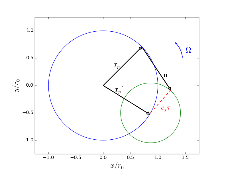
Consider an (infinite) uniform gaseous medium of density $\bar{\rho}_{g}$ and sound speed $c_{s}$. The medium is perturbed by a point mass in a fixed circular orbit of radius $r_{0}$ and angular velocity $\Omega>0$, in the $x-y$ plane. Let $\textbf{r}_{p}=\textbf{r}_{p}(t)$ and ${\textbf{r}_{p}}^{\prime}=\textbf{r}_{p}(t-\tau)$ be the position of the perturber at ”present-day” time $t$ and ”retarded” time $t^{\prime}=t-\tau$, respectively. We have $\textbf{r}_{p}(t)=r_{0}(\cos\Omega t\,\mathrm{\hat{\bf{x}}}+\sin\Omega t\,\mathrm{\hat{\bf{y}}})$. The Mach number is $\mathcal{M}\equiv v_{p}/c_{s}$, where $v_{p}=\Omega r_{0}$ is the perturber’s circular velocity. Furthermore, let u be the (three-dimensional) separation vector between $\textbf{r}_{p}(t)$ and the wavefront of the sound waves produced at time $t^{\prime}$ (see Fig. 1 for a schematic illustration).

Restricting the analysis to a linear response of the medium (Ostriker 1999, as in) leads to the driven sound wave equation

where $\alpha(\textbf{u},t)>0$ is the response fractional overdensity. The Green function method can be applied in various ways to solve for $\alpha(\textbf{u},t)$ and compute $\textbf{F}_{\text{DF}}(t)$. One possibility is to calculate $\alpha$ explicitly through the relation (Ostriker 1999)

The function $h(t)$ determines when the perturber is on or off. In a steady state we have $h=1$ at all times whereas, for a finite time perturbation, $h(t)=1$ for $t>0$ and zero otherwise. The retarded Green function $\frac{1}{r}\delta_{D}(\tau-r/c_{s})$ of the (sound) wave equation ensures causality, that is, the absence of solutions for $\tau<0$. The second equality, in which $\textbf{r}_{i}\equiv\textbf{r}_{p}(t)+\textbf{u}-\textbf{r}_{p}(t-\tau_{i})$ and $\textbf{v}_{i}\equiv\frac{d\textbf{r}_{p}}{dt}(t-\tau_{i})$, expresses $\alpha(\textbf{u},t)$ in terms of the Liénard-Wiechert (LW) potential (Landau & Lifshitz 1975, e.g.), a formulation convenient for numerical implementations. The roots $\tau_{i}$ are the time intervals for which the argument of the Dirac distribution vanishes. The drag force then follows from

Observe that $\textbf{F}_{\text{DF}}(t)$ is the gradient of a time-dependent potential so that $\oint\textbf{F}_{\text{DF}}\cdot d\textbf{r}\neq 0$.

In the supersonic case $\mathcal{M}>1$, the LW potential is singular on the Mach cone near the perturber (Kim & Kim 2007, see Appendix A of). More precisely, if $s=r_{0}\Omega\tau$ is the path length along the orbit (measured from the current perturber’s position), DF computed from the LW potential approximately scales as

in the vicinity of the perturber. Here, $\mathrm{\hat{\bf{r}}}(t)$ is a unit vector in the radial direction from the center of circular motion to the position of the perturber at $t$, and $\hat{\boldsymbol{\varphi}}(t)$ is a unit vector in the tangential direction (parallel to the velocity). Clearly, a divergence will arise in the $\hat{\boldsymbol{\varphi}}$-direction as $s\to 0$. This can be spotted in Fig. 2, which shows the density wake in the orbital plane of a perturber moving circularly with Mach number $\mathcal{M}=2$. Therefore, we expect that a Green function implementation recovers the radial DF, but generally fails at predicting the tangential DF in numerical investigations.

To tackle this complication, we consider a different route in which $\textbf{F}_{\text{DF}}(t)$ is evaluated directly. For this purpose, we express the retarded Green function as the Fourier transform (Landau & Lifshitz 1975; Jackson 1975, see)

where our convention is $\int_{\omega}\equiv\frac{1}{2\pi}\int_{-\infty}^{+\infty}\!d\omega$ and $\int_{\textbf{k}}=\frac{1}{(2\pi)^{3}}\int_{0}^{2\pi}\!d\varphi_{k}\int_{-1}^{+1}\!d\cos\vartheta_{k}\int_{-\infty}^{+\infty}\!dkk^{2}$ (in spherical coordinates $\textbf{k}=(k,\vartheta_{k},\varphi_{k})$). Moreover, $\epsilon>0$ so that the resonant poles (i.e. resonances) are in the lower-half of the complex $\omega$ plane to ensure causality. The advantages of a Fourier treatment over a configuration space approach are i) to bypass the computation of possibly singular LW potentials and ii) to regularize the resonances by contour deformation.

As we shall see shortly, the divergence at $\mathcal{M}>1$ remains, but it is encrypted in a maximum multipole $\ell_{\text{max}}$ that plays the role of small-scale cutoff.

We start from Eq. (3). After substituting $\frac{1}{r}\delta_{D}(\tau-r/c_{s})$ by its Fourier space expression (5), we replace both $e^{i\textbf{k}\cdot\textbf{r}_{p}}$ and $e^{-i\textbf{k}\cdot{\textbf{r}_{p}}^{\prime}}$ by their respective Rayleigh expansions (see Appendix §A for details of the calculation). However, we retain $e^{i\textbf{k}\cdot\textbf{u}}$ and take advantage of the Fourier transform of the Coulomb potential to perform the integral over u:

It is convenient to decompose the wavemode k onto the helicity basis $(\mathrm{\hat{\bf{z}}},\textbf{e}_{+},\textbf{e}_{-})$ where $\textbf{e}_{\pm}=\frac{1}{\sqrt{2}}\big(i\mathrm{\hat{\bf{y}}}\mp\mathrm{\hat{\bf{x}}}\big)$ are the positive and negative helicity modes. Namely,

with $Y_{l}^{m}(\mathrm{\hat{\bf{r}}})=Y_{l}^{m}(\vartheta,\varphi)$ being the usual spherical harmonics. Likewise, the drag force decomposes into

We must have $F^{(0)}\!(t)\equiv 0$ since the circular motion takes place in the plane $x-y$. Furthermore, we also have $F^{(+1)*}=-F^{(-1)}$ since the drag force is a real vector.

The Rayleigh expansions bring about factors of $Y_{l}^{m*}(\mathrm{\hat{\bf{r}}}_{p})$ and $Y_{l}^{m*}({\mathrm{\hat{\bf{r}}}_{p}}^{\prime})$. Since the azimuthal angle satisfies $\varphi_{p}-\varphi_{p}^{\prime}=\Omega\tau$, we find $Y_{l}^{m*}({\mathrm{\hat{\bf{r}}}_{p}}^{\prime})=e^{im\Omega\tau}Y_{l}^{m*}(\mathrm{\hat{\bf{r}}}_{p})$. On substituting this relation into the Rayleigh expansion of $e^{-i\textbf{k}\cdot{\textbf{r}_{p}}^{\prime}}$ and performing the angle integral over $\mathrm{\hat{\bf{k}}}$ (which reduces to the Gaunt integral), we arrive at

where the brackets denote Wigner 3j symbols, $j_{l}(x)$ are spherical Bessel functions, and

is the ”scattering” amplitude of radial (standing) waves. Note that $S_{l_{1},l_{2}}^{m_{2}*}=S_{l_{1},l_{2}}^{-m_{2}}$.

The symmetry properties of the Wigner 3j symbols imply that there is a non-vanishing contribution only if $\ell_{1}=\ell_{2}\pm 1$ so that $Y_{l_{1}}^{m_{1}*}(\mathrm{\hat{\bf{r}}}_{p})Y_{l_{2}}^{m_{2}*}(\mathrm{\hat{\bf{r}}}_{p})\propto e^{im\Omega t}$. This reflects conservation of angular momentum, and guarantees that DF has the same frequency $\Omega$ as the circular motion. Furthermore, one can check that the sum

vanishes identically for $m=0$ owing to the properties of the Wigner 3j symbols (they are non-zero only if $l_{1}+l_{2}+1$ is even) and to the fact that the polar angle is $\vartheta_{p}=\pi/2$. This ensures that the $z$-component of DF satisfies $F^{(0)}(t)\equiv 0$, as expected.

The components of DF in the helicity basis Eq. (8) can be recast into

In order to facilitate the comparison with Ostriker 1999, we have introduced the (generally complex) dimensionless function

Here, $P_{l}^{m}(x)$ are associated Legendre polynomials.

Using the properties of the Wigner 3j symbols and the associated Legendre polynomials, the dimensionality of the multiple sum can be reduced, and the function $I(\mathcal{M})$ thereby simplified to

which has much faster convergence than Eq. (II.2). This expression is valid both in the subsonic and supersonic regime.

The DF force eventually reads

where $\Re(I)$ and $\Im(I)$ are the real and imaginary part of $I(\mathcal{M})$. Eq. (21), together with $I(\mathcal{M})$ given by Eq. (20) and $S_{\ell,\ell-1}^{m}$ given by Eq. (13), is the central result of this paper.

The analyticity of the Green function along with the Sokhatsky-Weierstrass theorem

where $P$ denotes the Cauchy principal value, implies a connection between $\Re(I)$ and $\Im(I)$ or, equivalently, between the radial and tangential components of DF which is yet another manifestation of the Kramers-Kronig relations. However, while this implies that the real and imaginary part of the scattering amplitudes determine each other, the infinite sum (20) does not guarantee that both $\Re(I)$ and $\Im(I)$ are finite.

To illustrate this point, Fig. 3 displays $\Im(I)$ as a function of the maximum multipole $\ell_{\text{max}}$ at which the sum (20) is truncated, with $\ell_{\text{max}}$ as large as 500. Results are shown for a few values of $\mathcal{M}$. They demonstrate that $\Im(I)$ has a logarithmic divergence in the supersonic regime, in accordance with the numerical results of Kim & Kim 2007 and the recent analytical study of Fouvry et al. 2021. The magnitude of this divergence increases mildly with $\mathcal{M}$. In addition, we have numerically checked that $\Re(I)$ (not shown in Fig. 3) converges regardless of the value of $\mathcal{M}$.

This shows that our approach recovers the small-scale, Coulomb divergence rooted in the singular nature of the LW potentials in the supersonic regime, in agreement with the linear result (Ostriker 1999). The Fourier approach considered here has not removed this divergence, but the latter is now all encoded in the dependence of $I(\mathcal{M})$ on $\ell_{\text{max}}$. This will be helpful to assess the dependence of numerical simulations on resolution.

In steady-state, the integral over the time shift $\tau$ in Eq. (13) returns $(2\pi)\delta_{D}(m_{2}\Omega-\omega)$. This leaves us with a scattering amplitude $S_{l,l-1}^{m_{2}}(\mathcal{M})\equiv S_{l,l-1}^{\text{sty}}(m_{2}\mathcal{M})$ given by

where $z=kr_{0}$. To perform the integral, we expressed the spherical Bessel functions in terms of the Hankel functions $h_{l}^{(1)}\!(z)$ and $h_{l}^{(2)}\!(z)$, i.e. $j_{l}(z)=\frac{1}{2}(h_{l}^{(1)}\!(z)+h_{l}^{(2)}\!(z))$, and applied the method of Residues. Taking into account the contribution of a pole at $z=0$ to the contour integral of $h_{l_{1}}^{(1)}h_{l_{2}}^{(1)}$ (or $h_{l_{1}}^{(2)}h_{l_{2}}^{(2)}$), the resonant poles and the Wronskian $j_{l-1}(z)y_{l}(z)-j_{l}(z)y_{l-1}(z)=-\frac{1}{z^{2}}$ (here $y_{l}(z)$ is a modified spherical Bessel function) eventually lead to Eq. (III.1). When $m_{2}\mathcal{M}=0$, the scattering amplitude is solely controlled by the pole at the origin. In this case, taking the argument in Eq. (III.1) to zero yields

which agrees with a direct Residues calculation, as expected.

The scattering amplitude $S_{l,l-1}^{\text{sty}}\!(m_{2}\mathcal{M})$ converges to zero in the limit of large arguments. This happens so long as the azimuthal number $m_{2}$ is different from zero. When $m_{2}=0$, the argument is zero for any finite value of $\mathcal{M}$. As a result, only the terms with $m=0$ (from $S_{l,l-1}^{m}$) or $m=-1$ (from $-S_{l,l-1}^{m+1*}$) in the series expansion Eq. (20) survive when $\mathcal{M}\to\infty$. Since these are all proportional to $S_{l,l-1}(0)$, and since the steady-state amplitude $S_{l,l-1}^{\text{sty}}\!(0)$ is real and independent of $\mathcal{M}$, we must have $\Re(I)\to{\rm const}\,\mathcal{M}^{2}$ and $\Im(I)\to 0$ in the limit $\mathcal{M}\to\infty$.

The real and imaginary parts of $I(\mathcal{M})$ are displayed in Fig. 4. Our theoretical prediction (solid curves) is compared to the DF extracted from numerical schemes implementing the LW-based approach discussed in §II.1: triangles is data from Kim & Kim 2007, circles indicate our own simulation results (see Appendix §B for details). For $\Re(I)$, the agreement between theory and simulations is excellent, which demonstrates that the latter have converged. For $\Im(I)$ however, the numerical data depends on the actual resolution of the simulations which the Coulomb divergence is sensitive to. Truncating the series expansion (20) at multipole $\ell_{\text{max}}=12$ and 500 yields a reasonable fit to the two sets of simulations. The inferred values of $\ell_{\text{max}}$ are broadly consistent with the naive scaling $\ell_{\text{max}}\sim\pi/(r_{\text{min}}/r_{0})$, where the resolution is $r_{\text{min}}/r_{0}=0.1$ and $\simeq 7\times 10^{-3}$ in Kim & Kim 2007 and in our simulations, respectively.

While there is a short-distance (ultraviolet) divergence in the supersonic case, there is no long-distance (infrared) divergence at all in the circular case. To understand this, observe that the denominator of Eq. (III.1) saturates for $z\lesssim m_{2}\mathcal{M}$, i.e. $k\lesssim m_{2}/c_{s}T$ where $T$ is the orbital period, so that the integrand always vanishes in the limit $z\to 0$. In plain words, long-wavelength fluctuations do not contribute to the DF because they appear homogeneous to the circular perturber (the density pattern repeats itself on scales $\gtrsim c_{s}T$). This removes any long-distance (infrared) divergence.

Turning to the finite time perturbation, we have $h(t-\tau)=0$ for $\tau>t$. Consequently, the integral over the variable $\tau$ reduces to

As a result, the scattering amplitude is the sum $S_{l,l-1}^{\text{ftp},m_{2}}=S_{l,l-1}^{\text{sty},m_{2}}(\mathcal{M})+S_{l,l-1}^{\text{tra},m_{2}}\!(\mathcal{M},t)$, in which the transient contribution is the limit $\epsilon\to 0^{+}$ of

Here, $\tilde{t}=t/t_{\text{sc}}$ is in unit of the sound crossing time $t_{\text{sc}}=2r_{0}/c_{s}$. $S_{l,l-1}^{\text{tra},m_{2}}\!(\mathcal{M},t)$ can also be directly evaluated using the method of Residues. The decomposition of the integrand into a sum of products of Hankel functions reveals that the transient contribution vanishes for $\tilde{t}>1$, in agreement with the numerical findings of Kim & Kim 2007. This explains why, in the limit $\mathcal{M}\ll 1$, the steady-state circular solution $\Im(I)\approx\frac{1}{3}\mathcal{M}^{3}$ recovers the drag created by a linear trajectory perturber turned on at $t=0$: for $t_{\text{sc}}<t\ll t_{\text{sc}}/\mathcal{M}$, steady-state is achieved and, at the same time, $t$ is small enough that the motion is approximately linear.

Obtaining a compact expression for $S_{l,l-1}^{\text{tra},m_{2}}\!(\mathcal{M},t)$ is, however, challenging owing to the pole of order $2l+1$ at the origin.

The previous results straightforwardly extend to a compact binary on a circular orbit. We only need to take into account the presence of a second source at the antipode of $\textbf{r}_{p}^{\prime}$, that is, with an azimuthal angle $\varphi^{\prime}+\pi=\Omega(t-\tau)+\pi$. Let $M$ be the total binary mass and $q_{1}M$, $q_{2}M$ (with $q_{1}+q_{2}=1$) be the masses of the compact objects. Since the latter generally differ, so do their distances from the binary center-of-mass (assumed to be at rest relative to the gaseous medium). This affects the argument of the spherical Bessel functions in the Rayleigh expansion. For this purpose, we introduce the generalized amplitude

whose magnitude depends on whether $\alpha>\beta$ or $\alpha<\beta$. We find

and, in particular,

The computation proceeds along the lines of $S_{l,l-1}^{\text{sty}}\!(x)$. Exploiting a Wronskian relation of Bessel functions consistently returns $S_{l,l-1}^{\alpha,\alpha}\!(x)=\frac{i\pi}{2}j_{l}(\alpha x)h_{l}^{(1)}\!(\alpha x)$ in the special case $\alpha=\beta$.

We define the Mach number of the binary system as $\mathcal{M}=\Omega r_{0}/c_{s}$, where $r_{0}$ is the circular radius. The function $I(\mathcal{M})$ can be recast in the form Eq. (20) provided that the difference $S_{l,l-1}^{m}-S_{l,l-1}^{(m+1)*}$ in the numerator is replaced by

with $(\alpha,\beta)=(q_{2},q_{1})$ or $(q_{1},q_{2})$ depending on whether $I(\mathcal{M})$ encodes the DF acting on the compact object of mass $q_{1}M$ or its companion, respectively. The components of the DF can still be cast in the form of Eq. (15), except that $M$ now is the total mass of the compact binary. Like in the single perturber case, the tangential DF for a compact circular binary suffers from a small-scale logarithmic divergence.

To facilitate the comparison with Kim et al. 2008, who extended the approach of Kim & Kim 2007 to a compact binary, Fig. 5 displays our prediction for the equal mass case $q_{1}=q_{2}=1/2$ and assuming $\ell_{\text{max}}=12$ (the simulations of Kim et al. 2008 have the same resolution as those of Kim & Kim 2007). This low value of $\ell_{\text{max}}$ is responsible for the wiggles seen in the theoretical curves. Overall, our prediction closely track the smooth shape and the features seen in the numerical data of Kim et al. 2008.

References

- Annulli et al. (2020) Annulli, L., Cardoso, V., & Vicente, R. 2020, Phys. Rev. D, 102, 063022
- Banik & van den Bosch (2021) Banik, U., & van den Bosch, F. C. 2021, Astrophys. J., 912, 43
- Barausse (2007) Barausse, E. 2007, Mon. Not. Roy. Astron. Soc., 382, 826
- Berezhiani et al. (2019) Berezhiani, L., Elder, B., & Khoury, J. 2019, JCAP , 2019, 074
- Bondi & Hoyle (1944) Bondi, H., & Hoyle, F. 1944, Mon. Not. R. Astron. Soc., 104, 273
- Chandrasekhar (1943) Chandrasekhar, S. 1943, Astrophys. J., 97, 255
- Dokuchaev (1964) Dokuchaev, V. P. 1964, Soviet Astron., 8, 23
- Fouvry et al. (2021) Fouvry, J.-B., Hamilton, C., Rozier, S., & Pichon, C. 2021, Mon. Not. R. Astron. Soc., 508, 2210
- Hui et al. (2017) Hui, L., Ostriker, J. P., Tremaine, S., & Witten, E. 2017, Phys. Rev. D, 95, 043541
- Jackson (1975) Jackson, J. D. 1975, Classical electrodynamics (John Wiley & Sons)
- Just & Kegel (1990) Just, A., & Kegel, W. H. 1990, Astron. Astrophys., 232, 447
- Kaur & Sridhar (2018) Kaur, K., & Sridhar, S. 2018, Astrophys. J., 868, 134
- Kim & Kim (2007) Kim, H., & Kim, W.-T. 2007, Astrophys. J., 665, 432
- Kim et al. (2008) Kim, H., Kim, W.-T., & Sánchez-Salcedo, F. J. 2008, Astrophys. J. Lett., 679, L33
- Lancaster et al. (2020) Lancaster, L., Giovanetti, C., Mocz, P., et al. 2020, JCAP , 2020, 001
- Landau & Lifshitz (1975) Landau, L. D., & Lifshitz, E. M. 1975, The classical theory of fields (Elsevier Science & Technology)
- Lee & Stahler (2011) Lee, A. T., & Stahler, S. W. 2011, Mon. Not. R. Astron. Soc., 416, 3177
- Namouni (2010) Namouni, F. 2010, Mon. Not. R. Astron. Soc., 401, 319
- Ostriker (1999) Ostriker, E. C. 1999, Astrophys. J., 513, 252
- Rephaeli & Salpeter (1980) Rephaeli, Y., & Salpeter, E. E. 1980, Astrophys. J., 240, 20
- Ruderman & Spiegel (1971) Ruderman, M. A., & Spiegel, E. A. 1971, Astrophys. J., 165, 1
- Sánchez-Salcedo & Brandenburg (2001) Sánchez-Salcedo, F. J., & Brandenburg, A. 2001, Mon. Not. R. Astron. Soc., 322, 67
- Tremaine & Weinberg (1984) Tremaine, S., & Weinberg, M. D. 1984, Mon. Not. R. Astron. Soc., 209, 729