跳到论文正文
W Papers独立论文阅读器 arXiv:2111.07272 论文正文 计算阅读时间 · 0%
引用这篇论文根据当前论文元数据生成,正式投稿前建议核对。


License: arXiv.org perpetual non-exclusive license
arXiv:2111.07272v1 [math.NA] 14 Nov 2021

Numerical Analysis of the Multiple Scattering Theory for Electronic Structure Calculations Thanks:  X. Li and H. Chen’s work were partially supported by National Key R&D Program of China 2019YFA0709600, 2019YFA0709601. H. Chen’s work was partially supported by the Natural Science Foundation of China under grant 11971066. X. Gao’s work was partially supported by the Science Challenge Project under Grant TZ2018002.

Xiaoxu Li Thanks:  xiaoxuli@bnu.edu.cn, College of Education for the Future, Beijing Normal University.    Huajie Chen  and Xingyu Gao Thanks:  chen.huajie@bnu.edu.cn, School of Mathematical Sciences, Beijing Normal University. Thanks:  gao_xingyu@iapcm.ac.cn, Laboratory of Computational Physics, Institute of Applied Physics and Computational Mathematics.
Abstract

The multiple scattering theory (MST) is one of the most widely used methods in electronic structure calculations. It features a perfect separation between the atomic configurations and site potentials, and hence provides an efficient way to simulate defected and disordered systems. This work studies the MST methods from a numerical point of view and shows the convergence with respect to the truncation of the angular momentum summations, which is a fundamental approximation parameter for all MST methods. We provide both rigorous analysis and numerical experiments to illustrate the efficiency of the MST methods within the angular momentum representations.

1 Introduction

Multiple scattering theory (MST) was initiated to study the propagation of heat and electricity through inhomogeneous media [25]. It allows a unified treatment of many partial differential equations of modern physics and engineering, and has been applied to both classical and quantum physics, in particular, the electronic structure calculations of solid states. Along with the framework of density functional theory (DFT) [14, 16], MST has been successfully used to simulate the electronic structure of many systems, including bulk materials [1], surfaces [9], impurities [24] and alloys [22].

The idea of the MST methods is to divide the system into non-overlapping subregions, solve each of the smaller parts separately by quantum scattering theory, and then assembles the partial solutions of the pieces into an overall solution. A key feature of the MST method is that it affords a complete separation of the potential aspects from the structure aspects. Therefore, this approach is extremely potential to develop parallel algorithms for large and complex systems with substitutional defects, for example, the alloys [11, 29]. Another feature of the MST method is that it is a Green’s function method. Instead of solving the eigenvalue problems in standard electronic structure calculations, it can calculate the single-particle Green’s function directly. In the disordered systems, the statistical average of the Green’s function is the right object used to calculate the averaged physical properties, whereas the average of the wave function is not well-defined and cannot be directly related to the physical observables [8, 27].

The idea of MST to calculate the electronic structures was first known as the KKR method [15, 17], formulated by the so-called KKR secular equation, which can determine the eigenvalues and eigenstates of a many-particle system (see Section 2). Due to the huge computational cost, solving the original KKR equation is not widely used in practice nowadays. Nevertheless, it still founds the framework of the modern MST methods, by giving the so-called scattering path matrix, which is a key quantity to construct the Green’s function in almost all MST methods. We will only focus on the KKR method in this paper, but our theory (the error estimate of the angular-momentum truncations) is valid for all other practical MST methods.

The MST methods are always formulated and implemented within the angular-momentum representations. Therefore the accuracy of the MST solutions depends on the truncation of the angular-momentum summations. The convergence and error analysis of the solutions with respect to this truncation are thus crucial, which determine the reliability and efficiency of the MST simulation results. To our best knowledge, there is no existing work on rigorous mathematical analysis for the MST methods. We refer to [2, Section 5.10] for a non-rigorous discussion. The difficulties of analysis for the MST methods lie in two aspects. First, unlike the traditional discretization methods for electronic structure calculations (such as plane waves [3], finite elements [4], atomic orbitals [5, 13] and augmented plane waves [6, 28]), the MST methods are more of a perturbation method rather than a variational method, for which most of the standard approaches in numerical analysis fail. Second, the basic KKR secular equation is a highly nonlinear problem, where the coefficients in the equation have very complex dependence on the the energy to be solved.

The purpose of this paper is to derive an a priori error estimate of the MST solutions (i.e. the solutions of KKR secular equation) with respect to the angular-momentum truncations. We only consider linear Schrödinger-type eigenvalue problems in this paper, whereas the nonlinear problems deserve to be investigated in a separate work. The main result is the following superalgebraic convergence rate of the eigenpairs under certain assumptions (see Section 3 for details)

|EL−E|+‖uL−u‖≤Cs​L1−s∀s>1\displaystyle|E_{L}-E|+\|u_{L}-u\|\leq C_{s}L^{1-s}\hskip 20.00003pt\forall~s>1 (1.1)

where EE and uu are the energies (eigenvalues) and wave functions (eigenfunctions), LL is the angular-momentum cut-off, and the constant CsC_{s} only depends on the system and ss. The convergence result also works for other MST formulations (that are equivalent to the secular equation in math, but different in practice [11]).

Outline. The remainder of this paper is organized as follows. In Section 2, we give a brief overview of the multiple scattering theory. In particular, we consider the muffin-tin potentials and derive the KKR secular equation for linear Schrödinger-type eigenvalue problems within the angular-momentum representations. In Section 3, we provide a convergence analysis and an a priori error estimate of MST approximations (the solutions of the secular equations) with respect to the angular-momentum truncations. In Section 4, we present some numerical experiments to support the theory. In Section 5, we give some concluding remarks and future perspectives. For the sake of clarity of the presentations, the proofs and some supplementary details are put in the appendices.

Notations. Throughout the paper, we use the symbol CC to denote a generic positive constant that may change from one line to the next. In the error estimates, CC will always remain independent on the discretization parameters or the choice of test functions. The dependence of CC on model parameters will normally be clear from the context or stated explicitly.

Our analysis requires a number of notations for domain decompositions and special functions, and we list them in the following table with brief summaries. We also list the symbols that are frequently used in the paper.

General notations
𝒓,r,𝒓^\bm{r},~r,~\bm{\hat{r}} 𝒓∈ℝ3\bm{r}\in\mathbb{R}^{3} is the spatial coordinate, r=|𝒓|r=|\bm{r}| and 𝒓^=𝒓/r\bm{\hat{r}}=\bm{r}/r
𝒓n\bm{r}_{n} 𝒓n=𝒓−𝑹n\bm{r}_{n}=\bm{r}-\bm{R}_{n} with 𝑹n\bm{R}_{n} the position of the nn-th atom
ℓ,m\ell,~m angular-momenta and magnetic quantum numbers
LL angular-momentum truncation
z,zz,~\sqrt{z} zz is an energy parameter,  z:=i​|z|\sqrt{z}:=i\sqrt{|z|} if z<0z<0
E,u⁡(𝒓)E,~u(\bm{r}) bound state energy and wave function
EL,uL​(𝒓)E_{L},~u_{L}(\bm{r}) approximated bound state energy and wave function
∑ℓ​m,∑ℓ≤L\sum_{\ell m},~\sum_{\ell\leq L} ∑ℓ​m:=∑ℓ=0∞∑m=−ℓℓ,∑ℓ≤L:=∑ℓ=0L∑m=−ℓℓ\sum_{\ell m}:=\sum_{\ell=0}^{\infty}\sum_{m=-\ell}^{\ell},~~\sum_{\ell\leq L}:=\sum_{\ell=0}^{L}\sum_{m=-\ell}^{\ell}
Domain-related (see Figure 1.1)
ΩI\Omega^{\rm{I}} interstitial region
𝑹n\bm{R}_{n} position of the nn-th nucleus
Ωn,Rn,Γn\Omega_{n},~R_{n},~\Gamma_{n} atomic sphere centered at 𝑹n\bm{R}_{n}, its radius, and its surface
ΩnN\Omega^{\rm{N}}_{n} a neighbouring region around Ωn\Omega_{n} (see (2.13))
Bn,rnbB_{n},~r^{\rm b}_{n} a ring surrounding Ωn\Omega_{n} and its width (see page 3.2)
Function-related
Yℓ​m​(𝒓^)Y_{\ell m}(\hat{\bm{r}}) spherical harmonic functions
jℓ​(𝒓),nℓ​(𝒓),hℓ​(𝒓)j_{\ell}(\bm{r}),~n_{\ell}(\bm{r}),~h_{\ell}(\bm{r}) spherical Bessel, Neumann, and Hankel functions
Jℓ​m​(𝒓,z),Nℓ​m​(𝒓,z),Hℓ​m​(𝒓,z)J_{\ell m}(\bm{r};z),~N_{\ell m}(\bm{r};z),~H_{\ell m}(\bm{r};z) jℓ​(z​𝒓),nℓ​(z​𝒓),hℓ​(z​𝒓)j_{\ell}(\sqrt{z}\bm{r}),~n_{\ell}(\sqrt{z}\bm{r}),~h_{\ell}(\sqrt{z}\bm{r}) times Yℓ​m​(𝒓^)Y_{\ell m}(\hat{\bm{r}}) (see (2.10))
χℓ​(r,z)\chi_{\ell}(r;z) solution of the radial Schrödinger equation (see (2.5))
ζℓ​mn​(𝒓n,z)\zeta^{n}_{\ell m}(\bm{r}_{n};z) wave function in Ωn\Omega_{n} with energy parameter zz (see (2.20))
V⁡(𝒓)V(\bm{r}) potential of the system
V0​(r)V_{0}(r) a spherically symmetric potential centred at origin
MST-related
tℓ​(z)t_{\ell}(z) tt-matrix (see (2.6))
gℓ​m,ℓ′​m′n​n′​(z)g_{\ell m,\ell^{\prime}m^{\prime}}^{nn^{\prime}}(z) structure constants (see (2.15))
𝒰L​(z)\mathcal{U}_{L}(z), 𝒱L​(z)\mathcal{V}_{L}(z) functional spaces (see (3.6), (3.11))
ϕℓ​m,Ln​(𝒓,z)\phi_{\ell m,L}^{n}(\bm{r};z), φℓ​m,Ln​(𝒓,z)\varphi_{\ell m,L}^{n}(\bm{r};z) basis functions of 𝒰L​(z)\mathcal{U}_{L}(z) and 𝒱L​(z)\mathcal{V}_{L}(z) (see (3.2), (3.2))
ℳ\mathcal{M} a map from 𝒰L​(z)\mathcal{U}_{L}(z) to 𝒱L​(z)\mathcal{V}_{L}(z) (see (3.18))
ηn​(r)\eta_{n}(r) a cut-off function on BnB_{n} (see (3.2))
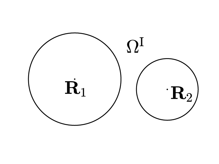
𝑹1\bm{R}_{1}Γ1\Gamma_{1}Ω1\Omega_{1}Ω1N\Omega^{N}_{1}𝑹2\bm{R}_{2}Γ2\Gamma_{2}Ω2\Omega_{2}B2B_{2}𝑹3\bm{R}_{3}Γ3\Gamma_{3}Ω3\Omega_{3}B3B_{3}ΩI\Omega^{\rm{I}}
Figure 1.1: Decomposition of the space into the atomic spheres and interstitial region.

2 Multiple scattering theory

In this section, we will apply multiple scattering theory to a Schrödinger-type equation and derive the KKR secular equation. Consider the following linear eigenvalue problem

(−Δ+V⁡(𝒓))​u​(𝒓)=E​u​(𝒓)𝒓∈ℝ3,\displaystyle\Big(-\Delta+V({\bm{r}})\Big)u({\bm{r}})=Eu({\bm{r}})\hskip 20.00003pt\bm{r}\in\mathbb{R}^{3}, (2.1)

where VV is the potential of the system, uu is subject to the boundary condition |u⁡(𝒓)|→0|u({\bm{r}})|\rightarrow 0 as |𝒓|→∞|\bm{r}|\rightarrow\infty (such that it is a bound state), and EE is the corresponding energy. In the following, we will focus on the case when VV is the so-called muffin-tin potentials, which are confined in non-overlapping spheres Ωn​(n=1,⋯,N)\Omega_{n}~(n=1,\cdots,N) centered at atomic sites 𝑹n\bm{R}_{n} with radius RnR_{n}. More precisely, the potential takes the form

V⁡(𝒓)=∑n=1Nvn​(|𝒓−𝑹n|)𝒓∈ℝ3,\displaystyle V({\bm{r}})=\sum_{n=1}^{N}v_{n}\big(|{\bm{r}}-{\bm{R}}_{n}|\big)\hskip 20.00003pt\bm{r}\in\mathbb{R}^{3}, (2.2)

with vn​(r)∈C∞​(0,∞)v_{n}(r)\in C^{\infty}(0,\infty) and vn​(r)=0v_{n}(r)=0 when r>Rnr>R_{n}. Here the potential has been assumed to be spherically symmetric within each atomic sphere only for simplicity of presentations. The analysis in this paper can be easily extended to general potentials that are non-spherically symmetric in the atomic spheres (see Appendix C).

The confinement that the potential is supported in atomic spheres is necessary for our analysis, which greatly simplifies the expressions of free electron propagator in the angular-momentum expansions. From a practical point of view, the MST algorithms can be generalized to arbitrary potentials by replacing the atomic spheres Ωn\Omega_{n} with the so-called space-filling cells (e.g. the Voronoi cell decompositions) [11], for which the mathematical formulations and numerical analysis are far more complicated. We will study the general cases (without interstitial region) in a separate work. We remark that the muffin-tin potential approximations not only allow dramatic simplifications for theoretical analysis and numerical algorithms, but also make very successful applications to many physical systems like metals and alloys [20, 23] where the use of the theory has continued until the present.

In our analysis, we will need to assume some regularity of the potential: V∈L2​(ℝ3)V\in L^{2}(\mathbb{R}^{3}) and V|Ωn∈C∞​((0,Rn)×𝕊2)V|_{\Omega_{n}}\in C^{\infty}((0,R_{n})\times\mathbb{S}^{2}). This is a mild assumption that can be satisfied in most of the physical problems of practical interests. For example, if the muffin-tin potential has singular Coulomb potential around the atomic sites, say vn​(r)≈C​r−1v_{n}(r)\approx Cr^{-1} near the origin, then the total potential VV satisfies this condition. It then follows from [26, p.119] that −Δ+V-\Delta+V has continuous spectrum on [0,+∞)[0,+\infty) and discrete spectrum below zero. We emphasize that we only consider the discrete spectrum E<0E<0 in this paper, which corresponds to the bound states of the system (2.1).

The approach of multiple scattering for solving (2.1) is usually formulated by two steps: (i) determining the relationship between the free electron gas and the system perturbed by a single atomic potential, and (ii) deriving a secular equation that connects the amplitudes of incoming and outgoing waves at multiple atomic sites.

2.1 Single-site scattering

Consider the following single-site scattering problem with a fixed energy parameter z<0z<0

(−Δ+V0​(r)−z)​ψ​(𝒓)=0𝒓∈ℝ3,\displaystyle\Big(-\Delta+V_{0}(r)-z\Big)\psi({\bm{r}})=0\hskip 20.00003pt\bm{r}\in\mathbb{R}^{3}, (2.3)

where the potential is spherically symmetric and can be written by a radial function V0V_{0} satisfying V0​(r)=0V_{0}(r)=0 for r≥R0r\geq R_{0}. Note that no (far-field) boundary condition is imposed on this equation, since we only concern the relationship between the incoming and outgoing waves by viewing the equation as a single potential scattering procedure. The solution ψ\psi depends on parameter zz, but we suppress this dependency throughout this paper for simplicity of presentations.

The solution ψ\psi can be written in the angular-momentum representation

ψ⁡(𝒓)=∑ℓ​mcℓ​m​χℓ​(r,z)​Yℓ​m​(𝒓^),\displaystyle\psi({\bm{r}})=\sum_{\ell m}c_{\ell m}\chi_{\ell}(r;z)Y_{\ell m}(\hat{\bm{r}}), (2.4)

where Yℓ​mY_{\ell m} is the spherical harmonic functions [12] and the radial part χℓ\chi_{\ell} satisfies the following radial Schrödinger equation at energy parameter zz

(∂2∂r2+2r​∂∂r−ℓ⁡(ℓ+1)r2−V0​(r)+z)​χℓ​(r,z)=0\displaystyle\displaystyle\left(\frac{\partial^{2}}{\partial r^{2}}+\frac{2}{r}\frac{\partial}{\partial r}-\frac{\ell(\ell+1)}{r^{2}}-V_{0}(r)+z\right)\chi_{\ell}(r;z)=0 0<r<R0,\displaystyle\hskip 20.00003pt0<r<R_{0}, (2.5a)
(∂2∂r2+2r​∂∂r−ℓ⁡(ℓ+1)r2+z)​χℓ​(r,z)=0\displaystyle\displaystyle\left(\frac{\partial^{2}}{\partial r^{2}}+\frac{2}{r}\frac{\partial}{\partial r}-\frac{\ell(\ell+1)}{r^{2}}+z\right)\chi_{\ell}(r;z)=0 r>R0.\displaystyle\hskip 20.00003ptr>R_{0}. (2.5b)

We first study (2.5b) outside the atomic sphere with vanishing potential, which is the well-known spherical Bessel differential equation [10]. For given ℓ∈ℕ\ell\in\mathbb{N} and z<0z<0, the solutions could be the spherical Bessel functions jℓ​(z​r)j_{\ell}(\sqrt{z}r), the spherical Newmann functions nℓ​(z​r)n_{\ell}(\sqrt{z}r), or the spherical Hankel functions hℓ​(z​r)=jℓ​(z​r)+i​nℓ​(z​r)h_{\ell}(\sqrt{z}r)=j_{\ell}(\sqrt{z}r)+in_{\ell}(\sqrt{z}r). The differences between these three special functions lie in their asymptotic behavior at the origin and infinity. For z<0z<0, the spherical Bessel functions jℓ​(z​r)j_{\ell}(\sqrt{z}r) are regular at the origin while the other two diverge, and the spherical Hankel functions hℓ​(z​r)h_{\ell}(\sqrt{z}r) are bounded at infinity while the other two are not (see, e.g. [10, 11]). Since any two of the above functions can make a complete basis set for the solutions of (2.5b), the radial solutions outside the atomic sphere can be represented by a linear combination of the spherical Bessel and Hankel functions

χℓ​(r,z)=aℓ​(z)​jℓ​(z​r)+bℓ​(z)​hℓ​(z​r)r≥R0.\displaystyle\chi_{\ell}(r;z)=a_{\ell}(z)j_{\ell}(\sqrt{z}r)+b_{\ell}(z)h_{\ell}(\sqrt{z}r)\hskip 20.00003ptr\geq R_{0}.

From a physical point of view, χℓ\chi_{\ell} can be viewed as a superposition of an incoming wave and a scattering wave, which correspond to the two parts with Bessel and Hankel functions, respectively.

The goal of single-site scattering is to determine the relationship between these two parts, more precisely, the ratio between the coefficients bℓb_{\ell} and aℓa_{\ell}

tℓ​(z):=bℓ​(z)aℓ​(z)for​ℓ∈ℕ.\displaystyle t_{\ell}(z):=\frac{b_{\ell}(z)}{a_{\ell}(z)}\hskip 20.00003pt\rm{for}~\ell\in\mathbb{N}. (2.6)

This gives the so-called tt-matrix (it is called a “matrix” since it is indexed by the angular momentum ℓ\ell for a given atomic site, and there are off-diagonal terms for non-spherical potential, see Appendix C) in MST method and is used as a fundamental building block of the whole theory.

From the numerical intuition, the tt-matrix can be determined by matching the values and derivatives of the radial solution χℓ\chi_{\ell} at r=R0r=R_{0}. Since multiplying χℓ\chi_{\ell} by an arbitrary constant does not change the solution of (2.5), it is only required to match the “logarithm derivatives” (log⁡(χℓ))′\big(\log(\chi_{\ell})\big)^{\prime} at r=R0r=R_{0}:

χℓ​(r,z)χℓ′​(r,z)|r=R0−=aℓ​(z)​jℓ​(z​r)+bℓ​(z)​hℓ​(z​r)z​aℓ​(z)​jℓ′​(z​r)+z​bℓ​(z)​hℓ′​(z​r)|r=R0+.\displaystyle\frac{\chi_{\ell}(r;z)}{\chi^{\prime}_{\ell}(r;z)}\bigg|_{r=R^{-}_{0}}=\frac{a_{\ell}(z)j_{\ell}(\sqrt{z}r)+b_{\ell}(z)h_{\ell}(\sqrt{z}r)}{\sqrt{z}a_{\ell}(z)j^{\prime}_{\ell}(\sqrt{z}r)+\sqrt{z}b_{\ell}(z)h^{\prime}_{\ell}(\sqrt{z}r)}\bigg|_{r=R^{+}_{0}}. (2.7)

Then a direct calculation with the definition (2.6) leads to

tℓ​(z)=z​χℓ​(R0,z)​jℓ′​(z​R0)−χℓ′​(R0,z)​jℓ​(z​R0)χℓ′​(R0,z)​hℓ​(z​R0)−z​χℓ​(R0,z)​hℓ′​(z​R0),\displaystyle t_{\ell}(z)=\frac{\sqrt{z}\chi_{\ell}(R_{0};z)j^{\prime}_{\ell}(\sqrt{z}R_{0})-\chi^{\prime}_{\ell}(R_{0};z)j_{\ell}(\sqrt{z}R_{0})}{\chi^{\prime}_{\ell}(R_{0};z)h_{\ell}(\sqrt{z}R_{0})-\sqrt{z}\chi_{\ell}(R_{0};z)h^{\prime}_{\ell}(\sqrt{z}R_{0})}, (2.8)

where we have denoted by χℓ′​(R0,z):=∂∂r​χℓ​(r,z)|r=R0−\chi^{\prime}_{\ell}(R_{0};z):=\frac{\partial}{\partial r}\chi_{\ell}(r;z)\big|_{r=R^{-}_{0}} the left-hand derivative of χℓ\chi_{\ell} at r=R0r=R_{0}. Note that the undetermined multiplicative constant involved in χℓ\chi_{\ell} can be canceled in (2.8), which leads to a unique tℓ​(z)t_{\ell}(z).

In the above matching procedure, a so-called “asymptotic problem” (see e.g. [6, 28]) with χℓ​(R0,z)=0\chi_{\ell}(R_{0};z)=0 must be avoided such that the conditions (2.7) and (2.8) can make sense. We will specify an explicit assumption to avoid this “asymptotic problem” later in Section 2.3.

An alternative way to derive the tt-matrix is to use the so-called Lippmann-Schwinger equation [11, 19, 20], which is the most widely-used approach in the quantum scattering theory. The Lippmann-Schwinger equation gives the relationship between incoming and outgoing waves via the free electron Green’s function, and writes the tt-matrix as

tℓ(z)=−iz∫0R0jℓ(zr)V0(r)χℓ(r;z)r2dr,\displaystyle t_{\ell}(z)=-i\sqrt{z}\int_{0}^{R_{0}}j_{\ell}(\sqrt{z}r)V_{0}(r)\chi_{\ell}(r;z)r^{2}{\rm d}r, (2.9)

where χℓ\chi_{\ell} is the solution of (2.5a) with some normalization condition. For the sake of completeness, we give a detailed explanation of (2.9) in Appendix B, and provide a rigorous analysis to show that the two expressions (2.8) and (2.9) for tt-matrix are equivalent. The integration form (2.9) from the Lippmann-Schwinger equation can be more easily generalized to non-spherical potentials (see Appendix C) and even arbitrary space-filling potentials (see [11]), which is therefore more widely used in practice. However, our analysis relies on the understanding of the matching condition (2.8).

2.2 Multiple-site scattering

The MST methods consider the eigenfunctions of (2.1) in the interstitial region as a wave scattered by the muffin-tin potential. For each atomic site, the incoming wave is expressed as the scattering waves from all other sites, while the resulting outgoing wave satisfies the single-site scattering relationship in the previous section. We will then briefly review how to derive the basic secular equation within this MST framework.

We first denote by

Hℓ​m​(𝒓,z)=hℓ​(z​r)​Yℓ​m​(𝒓^)andJℓ​m​(𝒓,z)=jℓ​(z​r)​Yℓ​m​(𝒓^)\displaystyle H_{\ell m}(\bm{r};z)=h_{\ell}\big(\sqrt{z}r\big)Y_{\ell m}(\hat{\bm{r}})\hskip 10.00002pt{\rm and}\hskip 10.00002ptJ_{\ell m}(\bm{r};z)=j_{\ell}\big(\sqrt{z}r\big)Y_{\ell m}(\hat{\bm{r}}) (2.10)

for ℓ∈ℕ\ell\in\mathbb{N} and |m|≤ℓ|m|\leq\ell. These functions give a complete basis set for the free-electron system with energy parameter zz. Then the eigenfunction uu of (2.1) (with corresponding eigenvalue EE) in the interstitial region can be written as a sum of scattering waves from all scattering center 𝑹n{\bm{R}}_{n},

u⁡(𝒓)=∑n=1N∑ℓ​mbℓ​mn​Hℓ​m​(𝒓n,E)𝒓∈ΩI\displaystyle u(\bm{r})=\sum_{n=1}^{N}\sum_{\ell m}b^{n}_{\ell m}H_{\ell m}(\bm{r}_{n};E)\hskip 20.00003pt\bm{r}\in\Omega^{\rm{I}} (2.11)

with the coefficients bℓ​mnb^{n}_{\ell m} and local coordinates 𝒓n:=𝒓−𝑹n{\bm{r}}_{n}:={\bm{r}}-{\bm{R}}_{n}. We only use the Hankel functions for the expansion (2.11) since hℓ​(E​r)h_{\ell}(\sqrt{E}r) is bounded at infinity for E<0E<0 while jℓ​(E​r)j_{\ell}(\sqrt{E}r) is not, so that the far-field boundary condition of (2.1) can be satisfied.

Alternatively, we can represent the eigenfunction as a superposition of incoming and outgoing waves around a specific atomic sphere. More precisely, for a given site 𝑹n\bm{R}_{n}, we write

u⁡(𝒓)=∑ℓ​m(aℓ​mn​Jℓ​m​(𝒓n,E)+bℓ​mn​Hℓ​m​(𝒓n,E))𝒓∈ΩnN\displaystyle u(\bm{r})=\sum_{\ell m}\big(a^{n}_{\ell m}J_{\ell m}(\bm{r}_{n};E)+b^{n}_{\ell m}H_{\ell m}(\bm{r}_{n};E)\big)\hskip 20.00003pt\bm{r}\in\Omega^{\rm{N}}_{n} (2.12)

with ΩnN⊂ΩI\Omega^{\rm{N}}_{n}\subset\Omega^{\rm I} the around nn-th atomic sphere (see Figure 1.1)

ΩnN={𝒓∈ΩI|Rn<|𝒓n|<minn′⁡{|𝑹n−𝑹n′|}}.\displaystyle\Omega^{\rm{N}}_{n}=\Big\{{\bm{r}}\in\Omega^{\rm I}~\Big|~R_{n}<|{\bm{r}}_{n}|<\min_{n^{\prime}}\{|\bm{R}_{n}-\bm{R}_{n^{\prime}}|\}\Big\}. (2.13)

We then have a so-called “expansion theorem” that can bridge the two expressions (2.11) and (2.12) for the eigenfunction u⁡(𝒓)u({\bm{r}}) in the interstitial region. For n′≠nn^{\prime}\neq n, the Hankel functions centered at atomic site 𝑹n\bm{R}_{n} can be expanded by the Bessel functions centered at 𝑹n′\bm{R}_{n^{\prime}}

Hℓ​m​(𝒓n,E)=∑ℓ′​m′gℓ​m,ℓ′​m′n​n′​(E)​Jℓ′​m′​(𝒓n′,E)𝒓∈Ωn′N,\displaystyle H_{\ell m}(\bm{r}_{n};E)=\sum_{\ell^{\prime}m^{\prime}}g_{\ell m,\ell^{\prime}m^{\prime}}^{nn^{\prime}}(E)J_{\ell^{\prime}m^{\prime}}(\bm{r}_{n^{\prime}};E)\hskip 20.00003pt\bm{r}\in\Omega^{\rm{N}}_{n^{\prime}}, (2.14)

where the coefficients gℓ​m,ℓ′​m′n​n′g_{\ell m,\ell^{\prime}m^{\prime}}^{nn^{\prime}} are the “structure constants” depending only on the energy parameter EE and the displacement between two atomic sites 𝑹n′−𝑹n\bm{R}_{n^{\prime}}-\bm{R}_{n}

gℓ​m,ℓ′​m′n​n′​(E)=4​π​∑ℓ′′​m′′il−l′−l′′​Cℓ​m,ℓ′​m′,ℓ′′​m′′​Hℓ′′​m′′​(𝑹n′−𝑹n,E)n≠n′\displaystyle g_{\ell m,\ell^{\prime}m^{\prime}}^{nn^{\prime}}(E)=4\pi\sum_{\ell^{\prime\prime}m^{\prime\prime}}i^{l-l^{\prime}-l^{\prime\prime}}C_{\ell m,\ell^{\prime}m^{\prime},\ell^{\prime\prime}m^{\prime\prime}}H_{\ell^{\prime\prime}m^{\prime\prime}}(\bm{R}_{n^{\prime}}-\bm{R}_{n};E)\hskip 20.00003ptn\neq n^{\prime} (2.15)

with Cℓ​m,ℓ′​m′,ℓ′′​m′′=∫S2Yℓ​m​(𝒓^)​Yℓ′​m′​(𝒓^)​Yℓ′′​m′′​(𝒓^)​𝑑𝒓^\displaystyle C_{\ell m,\ell^{\prime}m^{\prime},\ell^{\prime\prime}m^{\prime\prime}}=\int_{S^{2}}Y_{\ell m}(\hat{\bm{r}})Y_{\ell^{\prime}m^{\prime}}(\hat{\bm{r}})Y_{\ell^{\prime\prime}m^{\prime\prime}}(\hat{\bm{r}}){\rm d}\hat{\bm{r}} being the Gaunt coefficients [21]. By convention, the structure constant is set to be 00 for n=n′n=n^{\prime}. Note that the expansion (2.14) holds only in the region Ωn′N\Omega^{\rm{N}}_{n^{\prime}}, which is the reason we introduce this “neighbouring domain”. We refer to [11, Appendix D] for detailed discussions of the expansion (2.14).

Combining (2.11), (2.12), (2.14) and the symmetry of gℓ​m,ℓ′​m′n​n′​(E)g_{\ell m,\ell^{\prime}m^{\prime}}^{nn^{\prime}}(E) (i.e. gℓ​m,ℓ′​m′n​n′​(E)=gℓ′​m′,ℓ​mn′​n​(E)g_{\ell m,\ell^{\prime}m^{\prime}}^{nn^{\prime}}(E)=g_{\ell^{\prime}m^{\prime},\ell m}^{n^{\prime}n}(E)), we have that for any atomic site 𝑹n\boldsymbol{R}_{n},

aℓ​mn=∑n′≠n∑ℓ′​m′gℓ​m,ℓ′​m′n​n′​(E)​bℓ′​m′n′.\displaystyle a^{n}_{\ell m}=\sum_{n^{\prime}\neq n}\sum_{\ell^{\prime}m^{\prime}}g_{\ell m,\ell^{\prime}m^{\prime}}^{nn^{\prime}}(E)b^{n^{\prime}}_{\ell^{\prime}m^{\prime}}. (2.16)

Moreover, for each atomic site 𝑹n\boldsymbol{R}_{n}, the ratio between the coefficients aℓ​mna^{n}_{\ell m} and bℓ​mnb^{n}_{\ell m} has been given by the tt-matrix (2.6) of single-site scattering in the previous section

bℓ​mn=tℓn​(E)​aℓ​mn.\displaystyle b^{n}_{\ell m}=t^{n}_{\ell}(E)a^{n}_{\ell m}. (2.17)

Taking into accounts (2.16) and (2.17), we have the following equations

∑n′=1N∑ℓ′​m′(δℓ​ℓ′​δm​m′​δn​n′−tℓ′n′​(E)​gℓ​m,ℓ′​m′n​n′​(E))​aℓ′​m′n′=0for​n=1,⋯,N,ℓ=0,1,⋯,and−ℓ≤m≤ℓ.\qquad\sum_{n^{\prime}=1}^{N}\sum_{\ell^{\prime}m^{\prime}}\Big(\delta_{\ell\ell^{\prime}}\delta_{mm^{\prime}}\delta_{nn^{\prime}}-t^{n^{\prime}}_{\ell^{\prime}}(E)g_{\ell m,\ell^{\prime}m^{\prime}}^{nn^{\prime}}(E)\Big)a^{n^{\prime}}_{\ell^{\prime}m^{\prime}}=0\\ {\rm for}~n=1,\cdots,N,~\ell=0,1,\cdots,~{\rm and}~-\ell\leq m\leq\ell.\qquad (2.18)

In order to have non-trivial solutions of the system (2.18), we require EE to take the values such that the determinant of the coefficient matrix vanishes. This gives us the eigenvalues EE of the problem (2.1). Note that although (2.18) is derived for spherically symmetric potentials in this section, it can be easily generalized to non-spherical potentials within the muffin-tin form (see Appendix C).

2.3 The angular-momentum cut-off

Since (2.18) is in principle an infinite dimensional problem, one needs to truncate ℓ\ell to obtain a finite dimensional approximation in practical calculations. If the angular quantum number ℓ\ell is truncated by some cut-off LL, i.e. ℓ≤L\ell\leq L, then the solutions of (2.18) is approximated by ELE_{L} satisfying

Det⁡(S⁡(EL))=0,\displaystyle{\rm Det}\big(S(E_{L})\big)=0, (2.19)

where the matrix S⁡(EL)∈ℂ(N​(L+1)2)×(N​(L+1)2)S(E_{L})\in\mathbb{C}^{(N(L+1)^{2})\times(N(L+1)^{2})} is “truncated” from (2.18) with matrix elements

Sn​ℓ​m,n′​ℓ′​m′​(EL)=δℓ​ℓ′​δm​m′​δn​n′−tℓ′n′​(EL)​gℓ​m,ℓ′​m′n​n′​(EL).\displaystyle S_{n\ell m,n^{\prime}\ell^{\prime}m^{\prime}}(E_{L})=\delta_{\ell\ell^{\prime}}\delta_{mm^{\prime}}\delta_{nn^{\prime}}-t^{n^{\prime}}_{\ell^{\prime}}(E_{L})g_{\ell m,\ell^{\prime}m^{\prime}}^{nn^{\prime}}(E_{L}).

This is the so-called KKR secular equation that lays the foundation of MST methods. It is similar to an eigenvalue problem, in the sense that the “approximate eigenvalue” ELE_{L} yields a singular matrix S⁡(EL)S(E_{L}). However, (2.19) is very difficult to solve since the dependence of the matrix on ELE_{L} is highly nonlinear. One might resort to some “root-trace” algorithm (which is used in our numerical experiments, see Section 4 for details) to find the solution.

With the approximate solution ELE_{L}, the corresponding wave function inside each atomic sphere Ωn\Omega_{n} is given by

ζℓ​mn​(𝒓n,EL)=χℓn​(rn,EL)​Yℓ​m​(𝒓^n)|𝒓n|<Rn,\displaystyle\zeta^{n}_{\ell m}(\bm{r}_{n};E_{L})=\chi^{n}_{\ell}(r_{n};E_{L})Y_{\ell m}(\bm{\hat{r}}_{n})\hskip 20.00003pt|\bm{r}_{n}|<R_{n}, (2.20)

where χℓn\chi_{\ell}^{n} is the solution of (2.5a) satisfying the boundary condition

χℓn​(Rn,EL)=jℓ​(EL​Rn)+tℓn​(EL)​hℓ​(EL​Rn).\displaystyle\chi^{n}_{\ell}(R_{n};E_{L})=j_{\ell}(\sqrt{E_{L}}R_{n})+t^{n}_{\ell}(E_{L})h_{\ell}(\sqrt{E_{L}}R_{n}).

We then write the wave function as

uL​(𝒓,EL)={∑ℓ≤Laℓ​mn​(EL)​ζℓ​mn​(𝒓n,EL)𝒓∈Ωn​(n=1,⋯,N),∑n=1N∑ℓ≤Lbℓ​mn​(EL)​Hℓ​m​(𝒓n,EL)𝒓∈ΩI,\displaystyle u_{L}(\bm{r};E_{L})=\left\{\begin{array}[]{ll}\displaystyle\sum_{\ell\leq L}a^{n}_{\ell m}(E_{L})\zeta^{n}_{\ell m}(\bm{r}_{n};E_{L})&\quad\bm{r}\in\Omega_{n}~(n=1,\cdots,N),\\[4.30554pt] \displaystyle\sum_{n=1}^{N}\sum_{\ell\leq L}b^{n}_{\ell m}(E_{L})H_{\ell m}(\bm{r}_{n};E_{L})&\quad\bm{r}\in\Omega^{\rm I},\end{array}\right.

where the coefficients 𝒂:={aℓ​mn​(EL)}\boldsymbol{a}:=\{a^{n}_{\ell m}(E_{L})\} satisfies the equations

S⁡(EL)​𝒂=0\displaystyle S(E_{L})\boldsymbol{a}=0 (2.24)

with some normalization condition (for example, we can simply take ‖𝒂‖ℓ2=1\|\boldsymbol{a}\|_{\ell^{2}}=1), and bℓ​mn​(EL)=tℓn​(EL)​aℓ​mn​(EL)b^{n}_{\ell m}(E_{L})=t^{n}_{\ell}(E_{L})a^{n}_{\ell m}(E_{L}).

Throughout our analysis, we will make the following assumption

Det⁡(P⁡(EL))≠0,\displaystyle{\rm Det}\big(P(E_{L})\big)\neq 0, (2.25)

where the matrix P⁡(EL)∈ℂ(N​(L+1)2)×(N​(L+1)2)P(E_{L})\in\mathbb{C}^{(N(L+1)^{2})\times(N(L+1)^{2})} has elements

Pn​ℓ​m,n′​ℓ′​m′​(EL)=δn​n′​δℓ​ℓ′​δm​m′+jℓ′​(EL​Rn′)hℓ′​(EL​Rn′)​gℓ​m,ℓ′​m′n​n′​(EL).\displaystyle P_{n\ell m,n^{\prime}\ell^{\prime}m^{\prime}}(E_{L})=\delta_{nn^{\prime}}\delta_{\ell\ell^{\prime}}\delta_{mm^{\prime}}+\frac{j_{\ell^{\prime}}(\sqrt{E_{L}}R_{n^{\prime}})}{h_{\ell^{\prime}}(\sqrt{E_{L}}R_{n^{\prime}})}g_{\ell m,\ell^{\prime}m^{\prime}}^{nn^{\prime}}(E_{L}). (2.26)

This condition can make sure that the “asymptotic problem” χℓn​(Rn,z)=0​(n=1,⋯,N,ℓ≤LCLOSE\chi^{n}_{\ell}(R_{n};z)=0~(n=1,\cdots,N,\ell\leq L, see page 2.1) does not happen at energy parameter z=ELz=E_{L}. Note that if χℓn​(Rn,EL)=0\chi^{n}_{\ell}(R_{n};E_{L})=0, then (2.8) implies tℓn(EL)=−jℓ(ELRn)/hℓ(ELRn)t^{n}_{\ell}(E_{L})=-j_{\ell}(\sqrt{E_{L}}R_{n})/h_{\ell}(\sqrt{E_{L}}R_{n}), which makes S⁡(EL)=P⁡(EL)S(E_{L})=P(E_{L}) and leads to a contradiction between the KKR secular equation (2.19) and the assumption (2.25).

The angular-momentum truncation LL is the only numerical discretization parameter we have introduced so far, which is also the fundamental parameter for almost all MST methods. The goal of this work is to estimate the error from the truncation of angular-momentum sums. It has been observed in practical simulations that the truncation at relatively small number, say L=2L=2, L=3L=3, or L=4L=4, can already give satisfactory results in many cases of physical interest, such as that of metallic systems on close-packed lattices [11]. The fast convergence with respect to LL derived in the following section can provide a theoretical justification for this phenomenon.

3 Numerical analysis of the MST approximations

In this section, we will present an error estimate for the solutions of (2.19) with respect to the angular-momentum cut-off LL. The analysis consists of three steps. First, we characterize the (approximate) solution space of the KKR secular equation, in particular, we give the weak continuity condition of (2.3) through atomic spherical surfaces. Then we convert the KKR secular equation into an equivalent variational form, whose solutions are exactly the same as those of KKR secular equation. Finally we provide a convergence analysis for the equivalent variational form and obtain a spectral convergence rate.

We consider the following weak form of eigenvalue problem (2.1): Find E∈ℝE\in\mathbb{R} and u∈H1​(ℝ3)u\in H^{1}(\mathbb{R}^{3}) such that ‖u‖L2​(ℝ3)=1\|u\|_{L^{2}(\mathbb{R}^{3})}=1 and

a⁡(u,v)=E⁡(u,v)∀v∈H1​(ℝ3),\displaystyle a(u,v)=E(u,v)\hskip 20.00003pt\forall~v\in H^{1}(\mathbb{R}^{3}), (3.1)

where the bilinear form a⁡(⋅,⋅):H1​(ℝ3)×H1​(ℝ3)→ℂa(\cdot,\cdot):H^{1}(\mathbb{R}^{3})\times H^{1}(\mathbb{R}^{3})\rightarrow\mathbb{C} is defined by

a⁡(u,v):=∫ℝ3∇u⋅∇v∗+V​u​v∗\displaystyle a(u,v):=\int_{\mathbb{R}^{3}}\nabla u\cdot\nabla v^{*}+Vuv^{*}

with asterisk denoting the conjugate. This bilinear form is coercive on H1​(ℝ3)H^{1}(\mathbb{R}^{3}), i.e., there exist positive constants α\alpha and β\beta such that

a⁡(v,v)≥α​‖v‖H1​(ℝ3)2−β​‖v‖L2​(ℝ3)2∀v∈H1​(ℝ3).\displaystyle a(v,v)\geq\alpha\|v\|^{2}_{H^{1}(\mathbb{R}^{3})}-\beta\|v\|^{2}_{L^{2}(\mathbb{R}^{3})}\hskip 20.00003pt\forall~v\in H^{1}(\mathbb{R}^{3}). (3.2)

For simplicity, we will assume β=0\beta=0 afterwards since a shifted bilinear form aβ​(u,v):=a⁡(u,v)+β⁡(u,v)a^{\beta}(u,v):=a(u,v)+\beta(u,v) makes no essential change to the eigenvalue problem.

3.1 Approximate wave function space

We define the following space related to the muffin-tin decomposition

Hδ(ℝ3)={v∈L2(ℝ3)|v|ΩI∈H1(ΩI),v|Ωn∈H1(Ωn)∀1≤n≤N},\displaystyle H^{\delta}(\mathbb{R}^{3})=\left\{v\in L^{2}(\mathbb{R}^{3})~\Big|~v|_{\Omega^{\rm I}}\in H^{1}(\Omega^{\rm I}),~v|_{\Omega_{n}}\in H^{1}(\Omega_{n})~~\forall~1\leq n\leq N\right\},

with a broken Sobolev norm ‖v‖δ=‖v‖H1​(ΩI)+∑n=1N‖v‖H1​(Ωn)\|v\|_{\delta}=\|v\|_{H^{1}(\Omega^{\rm I})}+\sum_{n=1}^{N}\|v\|_{H^{1}(\Omega_{n})}, We further define a bilinear form aδ​(⋅,⋅):Hδ​(ℝ3)×Hδ​(ℝ3)→ℂa_{\delta}(\cdot,\cdot):H^{\delta}(\mathbb{R}^{3})\times H^{\delta}(\mathbb{R}^{3})\rightarrow\mathbb{C} by

aδ​(u,v):=∫ΩI∇u⋅∇v∗+∑n=1N∫Ωn∇u⋅∇v∗+∫ℝ3V​u​v∗.\displaystyle a_{\delta}(u,v):=\int_{\Omega^{\rm I}}\nabla u\cdot\nabla v^{*}+\sum_{n=1}^{N}\int_{\Omega_{n}}\nabla u\cdot\nabla v^{*}+\int_{\mathbb{R}^{3}}Vuv^{*}.

Inherited from the coercivity of a⁡(⋅,⋅)a(\cdot,\cdot) in (3.2), we have that there exist αδ>0\alpha_{\delta}>0 such that

aδ​(v,v)≥αδ​‖v‖δ2∀v∈Hδ​(ℝ3).\displaystyle a_{\delta}(v,v)\geq\alpha_{\delta}\|v\|^{2}_{\delta}\hskip 20.00003pt\forall~v\in H^{\delta}(\mathbb{R}^{3}).

We introduce the notion of “weak continuity” for the functions in Hδ​(ℝ3)H^{\delta}(\mathbb{R}^{3}) that are continuous through the atomic spherical surfaces Γn​(n=1,⋯,N)\Gamma_{n}~(n=1,\cdots,N) for low angular-momentum components. For v∈Hδ​(ℝ3)v\in H^{\delta}(\mathbb{R}^{3}), we denote by [v]Γn:=v+|Γn−v−|Γn[v]_{\Gamma_{n}}:=v^{+}|_{\Gamma_{n}}-v^{-}|_{\Gamma_{n}} the jump through surface Γn\Gamma_{n}, where v±|Γnv^{\pm}|_{\Gamma_{n}} denote the traces of vv taken from inside and outside the sphere Ωn\Omega_{n}, respectively. For a given L≥0L\geq 0, we say that vv is weakly continuous through Γn\Gamma_{n} if

∫Γn[v]Γn​Yℓ​m​(𝒓^)​𝑑𝒓^=0∀0≤ℓ≤L,|m|≤ℓ.\displaystyle\int_{\Gamma_{n}}[v]_{\Gamma_{n}}Y_{\ell m}(\hat{\bm{r}}){\rm d}\hat{\bm{r}}=0\hskip 20.00003pt\forall~0\leq\ell\leq L,~|m|\leq\ell. (3.3)

We then consider the following finite dimensional space with given angular-momentum truncation LL and energy parameter zz

𝒲L(z)={ψ∈Hδ(ℝ3)|ψ|ΩI=∑n=1N∑ℓ≤Lc~n​ℓ​mHℓ​m(𝒓n;z),ψ|Ωn=∑n=1N∑ℓ≤Lc¯n​ℓ​mζnℓ​m(𝒓n;z),ψand∂ψ∂rnsatisfy (3.3) forn=1,⋯,N},\mathcal{W}_{L}(z)=\Big\{\psi\in H^{\delta}(\mathbb{R}^{3})~\Big|~\psi|_{\Omega^{\rm I}}=\sum_{n=1}^{N}\sum_{\ell\leq L}\tilde{c}_{n\ell m}H_{\ell m}(\bm{r}_{n};z),~\\[4.30554pt] \psi|_{\Omega_{n}}=\sum_{n=1}^{N}\sum_{\ell\leq L}\bar{c}_{n\ell m}\zeta^{n}_{\ell m}(\bm{r}_{n};z),~\psi~{\rm and}~\frac{\partial\psi}{\partial r_{n}}~\text{satisfy \eqref{mortar-value} }{\rm for}~n=1,\cdots,N\Big\},\qquad (3.4)

where c~n​ℓ​m\tilde{c}_{n\ell m} and c¯n​ℓ​m\bar{c}_{n\ell m} are coefficients, ζℓ​mn\zeta^{n}_{\ell m} is given by (2.20), and ∂/∂rn\displaystyle\partial/\partial r_{n} denotes the derivative along the radial direction with respect to the nn-th atomic site 𝑹n\bm{R}_{n}. It is obvious that the functions in 𝒲L​(z)\mathcal{W}_{L}(z) satisfy the following strong form in the interstitial region and atomic spheres, respectively

(−Δ+V⁡(𝐫)−z)​uL​(𝒓,z)=0𝒓∈ℝ3\(⋃n=1NΓn).\displaystyle(-\Delta+V({\bf r})-z)u_{L}({\bm{r}};z)=0\displaystyle\hskip 20.00003pt\bm{r}\in\mathbb{R}^{3}\backslash\left(\bigcup_{n=1}^{N}\Gamma_{n}\right). (3.5)

The solutions uLu_{L} inside and outside the spheres are then patched together through Γn\Gamma_{n} by the weak continuity conditions (3.3).

Note that the space 𝒲L​(z)\mathcal{W}_{L}(z) is trivial (only contains zero function) for most of the energy parameter zz, and non-trivial only for the solution z=ELz=E_{L} of the KKR secular equation (2.19). This is justified in the following lemma, whose proof is given in Appendix A.1.

Lemma 3.1.

ELE_{L} solves (2.19) if and only if 𝒲L​(EL)\{0}≠∅\mathcal{W}_{L}(E_{L})\backslash\{0\}\neq\emptyset. Moreover, if ELE_{L} solves (2.19), then 𝒲L​(EL)={u∈Hδ​(ℝ3)|u​ can be written as (2.3)}\mathcal{W}_{L}(E_{L})=\big\{u\in H^{\delta}(\mathbb{R}^{3})~\big|~u\text{ can be written as \eqref{kkr-wavefun}}\big\}.

3.2 Equivalent variational form

In this subsection, we will construct an eigenvalue problem in a variational form, whose eigenvalues can be shown to be the same as the solutions of the KKR secular equation (2.19).

For a given energy parameter zz, we define the trial function space

𝒰L​(z)={u∈Hδ​(ℝ3)|u=∑n=1N∑ℓ≤Lcn​ℓ​m​ϕℓ​m,Ln​(𝒓,z)},\displaystyle\mathcal{U}_{L}(z)=\left\{u\in H^{\delta}(\mathbb{R}^{3})~\Big|~u=\sum_{n=1}^{N}\sum_{\ell\leq L}c_{n\ell m}\phi_{\ell m,L}^{n}(\bm{r};z)\right\}, (3.6)

where the basis function ϕℓ​m,Ln\phi_{\ell m,L}^{n} is given by

ϕℓ​m,Ln​(𝒓,z)={Hℓ​m​(𝒓n,z)in​ΩI,hℓ​(z​Rn)​ζℓ​mn​(𝒓n,z)in​Ωn,∑ℓ′≤L(gℓ​m,ℓ′​m′n​n′​(z)​jℓ′​(z​Rn′))​ζℓ′​m′n′​(𝒓n′,z)in​Ωn′∀n′≠n.\displaystyle\phi_{\ell m,L}^{n}(\bm{r};z)=\left\{\begin{array}[]{ll}H_{\ell m}({\bm{r}_{n}};z)&{\rm in}~\Omega^{\rm I},\\[4.30554pt] h_{\ell}(\sqrt{z}R_{n})\zeta_{\ell m}^{n}(\bm{r}_{n};z)&{\rm in}~\Omega_{n},\\[4.30554pt] \displaystyle\sum_{\ell^{\prime}\leq L}\Big(g_{\ell m,\ell^{\prime}m^{\prime}}^{nn^{\prime}}(z)j_{\ell^{\prime}}(\sqrt{z}R_{n^{\prime}})\Big)\zeta_{\ell^{\prime}m^{\prime}}^{n^{\prime}}(\bm{r}_{n^{\prime}};z)&{\rm in}~\Omega_{n^{\prime}}\quad\forall~n^{\prime}\neq n.\end{array}\right.

The basis function ϕℓ​m,Ln\phi_{\ell m,L}^{n} is constructed as (3.2) such that it (a) is the solution of radial Schrödinger equation at energy zz times spherical harmonic function Yℓ​mY_{\ell m} in the nn-th atomic sphere, (b) extends to the interstitial region continuously by Hankel functions Hℓ​mH_{\ell m} as the scattered wave, (c) and flows into other atomic spheres in a weakly continuous way while satisfying the Schrödinger equation with energy zz at the same time. Therefore, 𝒲L​(z)\mathcal{W}_{L}(z) is a subset of 𝒰L​(z)\mathcal{U}_{L}(z). Conversely, 𝒰L​(z)\mathcal{U}_{L}(z) contains more functions than 𝒲L​(z)\mathcal{W}_{L}(z), say 𝒲L​(z)⊊𝒰L​(z)\mathcal{W}_{L}(z)\subsetneq\mathcal{U}_{L}(z), since the slope of ϕℓ​m,Ln\phi_{\ell m,L}^{n} may not be weakly continuous through the atomic spherical surfaces.

We also need the following test function space

𝒱L​(z)={u∈Hδ​(ℝ3)|u=∑n=1N∑ℓ≤Lcn​ℓ​m​φℓ​m,Ln​(𝒓,z)},\displaystyle\mathcal{V}_{L}(z)=\left\{u\in H^{\delta}(\mathbb{R}^{3})~\Big|~u=\sum_{n=1}^{N}\sum_{\ell\leq L}c_{n\ell m}\varphi_{\ell m,L}^{n}(\bm{r};z)\right\}, (3.11)

where the basis function φℓ​m,Ln\varphi_{\ell m,L}^{n} is defined by

φℓ​m,Ln​(𝒓,z)={ϕℓ​m,Ln​(𝒓,z)−ηn′​(|𝒓n′|)​∑ℓ′>Lgℓ​m,ℓ′​m′n​n′​(z)​Jℓ′​m′​(𝒓n′,z)in​Bn′​(n′≠n),ϕℓ​m,Ln​(𝒓,z)otherwise\displaystyle\varphi_{\ell m,L}^{n}(\bm{r};z)=\left\{\begin{array}[]{ll}\displaystyle\phi_{\ell m,L}^{n}(\bm{r};z)-\eta_{n^{\prime}}(|\bm{r}_{n^{\prime}}|)\sum_{\ell^{\prime}>L}g_{\ell m,\ell^{\prime}m^{\prime}}^{nn^{\prime}}(z)J_{\ell^{\prime}m^{\prime}}(\bm{r}_{n^{\prime}};z)&{\rm in}~B_{n^{\prime}}~(n^{\prime}\neq n),\\[4.30554pt] \phi_{\ell m,L}^{n}(\bm{r};z)&{\rm otherwise}\end{array}\right.~~

with Bn={𝒓|Rn<|𝒓n|<Rn+rnb}B_{n}=\{{\bm{r}}~\big|~R_{n}<|{\bm{r}}_{n}|<R_{n}+r_{n}^{\rm b}\} being a ring (of width rnbr_{n}^{\rm b}) around the nn-th atomic sphere (see Figure 1.1), and ηn\eta_{n} being a cut-off functions satisfying ηn∈C∞[0,+∞)\eta_{n}\in C^{\infty}[0,+\infty), 0≤ηn≤10\leq\eta_{n}\leq 1 and

ηn​(r)={1r≤Rn0r≥Rn+rnbfor​n=1,⋯,N.\displaystyle\eta_{n}(r)=\left\{\begin{array}[]{ll}1&\quad r\leq R_{n}\\[4.30554pt] 0&\quad r\geq R_{n}+r_{n}^{\rm b}\end{array}\right.\hskip 10.00002pt{\rm for}~n=1,\cdots,N.

The widths rnbr_{n}^{\rm b} should be small enough such that the regions Bn​(n=1,⋯,N)B_{n}~(n=1,\cdots,N) do not overlap. The basis function φℓ​m,Ln\varphi_{\ell m,L}^{n} can be viewed as a slight mollification of ϕℓ​m,Ln\phi_{\ell m,L}^{n} (only on the regions Bn′B_{n^{\prime}} with n′≠nn^{\prime}\neq n) by the cut-off functions, such that it is continuous (not just weakly continuous) through the atomic spherical surfaces Γn′\Gamma_{n^{\prime}}. Note that φℓ​m,Ln\varphi_{\ell m,L}^{n} does not satisfy the Schrödinger equation in BnB_{n} any more.

We then define a map ℳ:𝒰L​(z)→𝒱L​(z)\mathcal{M}:\mathcal{U}_{L}(z)\rightarrow\mathcal{V}_{L}(z) such that

ℳ​ϕℓ​m,Ln​(𝒓,z)=φℓ​m,Ln​(𝒓,z)∀1≤n≤N,0≤ℓ≤L,|m|≤ℓ.\displaystyle\mathcal{M}\phi_{\ell m,L}^{n}(\bm{r};z)=\varphi_{\ell m,L}^{n}(\bm{r};z)\hskip 20.00003pt\forall~1\leq n\leq N,~0\leq\ell\leq L,~|m|\leq\ell. (3.18)

It can be seen from the definition that the role of ℳ\mathcal{M} is to mollify the functions in 𝒰L​(z)\mathcal{U}_{L}(z) from weakly continuous to continuous through the atomic spherical surfaces. Note that the mapping ℳ\mathcal{M} actually depends on the energy parameter zz and the angular-momentum truncation LL. For simplicity of presentations, we will suppress this dependence whenever it is clear from the context.

We then construct the following variational form of an eigenvalue problem: Find EL∈ℝE_{L}\in\mathbb{R} and uL∈𝒰L​(EL)u_{L}\in\mathcal{U}_{L}(E_{L}) such that (uL,ℳ​uL)=1(u_{L},\mathcal{M}u_{L})=1 and

aL​(uL,v)=EL​(uL,ℳ​v)∀v∈𝒰L​(EL),\displaystyle a_{L}(u_{L},v)=E_{L}(u_{L},\mathcal{M}v)\hskip 20.00003pt\forall~v\in\mathcal{U}_{L}(E_{L}), (3.19)

where the bilinear form aL​(⋅,⋅):𝒰L​(z)×𝒰L​(z)→ℂa_{L}(\cdot,\cdot):~\mathcal{U}_{L}(z)\times\mathcal{U}_{L}(z)\rightarrow\mathbb{C} is defined by

aL​(u,v):=aδ​(u,ℳ​v).\displaystyle a_{L}(u,v):=a_{\delta}(u,\mathcal{M}v).

We mention that (3.19) can also be viewed as a Petrov-Galerkin scheme [7]: Find EL∈ℝE_{L}\in\mathbb{R} and uL∈𝒰L​(EL)u_{L}\in\mathcal{U}_{L}(E_{L}) such that (uL,ℳ​uL)=1(u_{L},\mathcal{M}u_{L})=1 and

aδ​(uL,v)=EL​(uL,v)∀v∈𝒱L​(EL),\displaystyle a_{\delta}(u_{L},v)=E_{L}(u_{L},v)\hskip 20.00003pt\forall~v\in\mathcal{V}_{L}(E_{L}),

where the trial function space 𝒰L​(z)\mathcal{U}_{L}(z) and the test function space 𝒱L​(z)\mathcal{V}_{L}(z) are (slightly) different.

Note that (3.19) is a nonlinear eigenvalue problem since both the bilinear form aL​(⋅,⋅)a_{L}(\cdot,\cdot) and the trial function space 𝒰L​(EL)\mathcal{U}_{L}(E_{L}) depend on the eigenvalue ELE_{L} under consideration. Therefore the solution may be very difficult to find from a practical point of view. However, we clarify that (3.19) is introduced only for theoretical analysis rather than practical calculations.

We will first show some basic properties of the bilinear form aL​(⋅,⋅)a_{L}(\cdot,\cdot) in the following lemma, which implies that aLa_{L} gives an inner product on 𝒰L​(z)\mathcal{U}_{L}(z), and is coercive and continuous with respect to the broken Sobolev norm ∥⋅∥δ\|\cdot\|_{\delta}. The proof is given in Appendix A.2.

Lemma 3.2.

(a) aL​(⋅,⋅)a_{L}(\cdot,\cdot) is symmetric, i.e.,

aL​(u,v)=aL​(v,u)∗∀u,v∈𝒰L​(z).\displaystyle a_{L}(u,v)=a_{L}(v,u)^{*}\hskip 20.00003pt\forall~u,v\in\mathcal{U}_{L}(z). (3.20)

(b) If LL is sufficiently large, then there exist positive constants C1,C2,C3C_{1},~C_{2},~C_{3} and C4C_{4} that do not depend on LL, such that for any u∈𝒰L​(z)u\in\mathcal{U}_{L}(z),

(b1)C1​‖u‖δ2≤aL​(u,u)≤C2​‖u‖δ2,\displaystyle{\rm(b1)}\hskip 20.00003ptC_{1}\|u\|^{2}_{\delta}\leq a_{L}(u,u)\leq C_{2}\|u\|^{2}_{\delta}, (3.21)
(b2)‖ℳ​u‖L2​(ℝ3)≤C3​‖u‖L2​(ℝ3)and‖ℳ​u‖δ≤C4​‖u‖δ.\displaystyle{\rm(b2)}\hskip 20.00003pt\|\mathcal{M}u\|_{L^{2}(\mathbb{R}^{3})}\leq C_{3}\|u\|_{L^{2}(\mathbb{R}^{3})}\hskip 20.00003pt{\rm and}\hskip 20.00003pt\|\mathcal{M}u\|_{\delta}\leq C_{4}\|u\|_{\delta}. (3.22)

Then we can derive the following theorem, which shows that the solutions of the KKR secular equation are equivalent to those of the variational form (3.19). The proof is given in Appendix A.3.

Theorem 3.1.

If the asymptotic assumption (2.25) is satisfied, then the following two statements are equivalent: (a) (EL,uL)(E_{L},u_{L}) is an eigenpair of (3.19); (b) ELE_{L} is a solution of (2.19) and uLu_{L} is given by (2.3).

With this key observation, the error estimates for the KKR equation can now be obtained from the analysis of the variational problem. From this theorem, we see that although the choice of cutoff ηn\eta_{n} affects the construction of the test function space 𝒱L​(z)\mathcal{V}_{L}(z) as well as the operator ℳ\mathcal{M}, but the solutions of (3.19) do not depend on ηn\eta_{n}.

3.3 Convergence and a prior error estimates

Let (EL,uL)(E_{L},u_{L}) solves (3.19) with the angular-momentum truncation L∈ℕL\in\mathbb{N}. We will provide an error estimate for the approximate error with respect to LL.

Due to the coercivity of aL​(⋅,⋅)a_{L}(\cdot,\cdot) stated in Lemma 3.2, the approximate eigenvalues ELE_{L} have a lower bound. Note that we search the eigenvalue approximations in a finite energy window that contains the eigenvalues to be calculated, we will have limiting points in this region. We will show that any limiting point is an eigenvalue of the original problem (3.1) and possesses some spectral convergence rate.

Let E∞∈ℝE_{\infty}\in\mathbb{R} be any accumulation point, that is, there exists a subsequence {ELj}j∈ℤ+\{E_{L_{j}}\}_{j\in\mathbb{Z}_{+}} converge to E∞E_{\infty}

limj→∞|ELj−E∞|=0.\displaystyle\lim\limits_{j\rightarrow\infty}\big|E_{L_{j}}-E_{\infty}\big|=0. (3.23)

Then it follows from the coercivity in Lemma 3.2 that

ELj=aLj​(uLj,uLj)≥C​‖uLj‖δ2,\displaystyle E_{L_{j}}=a_{L_{j}}(u_{L_{j}},u_{L_{j}})\geq C\|u_{L_{j}}\|^{2}_{\delta}, (3.24)

which indicates that uLju_{L_{j}} is bounded in Hδ​(ℝ3)H^{\delta}(\mathbb{R}^{3}). Consequently, there exists a weakly convergent subsequence {uLjk}k∈ℤ+\{u_{L_{j_{k}}}\}_{k\in\mathbb{Z}_{+}}, such that

uLjk⇀u∞in​Hδ​(ℝ3)as​k→∞.\displaystyle u_{L_{j_{k}}}\rightharpoonup u_{\infty}\hskip 10.00002pt\text{in}~H^{\delta}(\mathbb{R}^{3})\hskip 10.00002pt\text{as}~k\rightarrow\infty. (3.25)

For simplicity of the presentation, we will still denote the weakly converged subsequence uLjku_{L_{j_{k}}} by uLu_{L} in the following.

The next theorem is the main result of this paper, which shows that the limiting pair (E∞,u∞)(E_{\infty},u_{\infty}) is an eigenpair of the eigenvalue problem (3.1), and the KKR approximations (i.e. the solutions of (3.19) or (2.19)) converge to the eigenpair super-algebraically fast as LL increases. The proof of this theorem is given in Appendix A.4.

Theorem 3.2.

Any limiting pair (E∞,u∞)(E_{\infty},u_{\infty}) is an eigenpair of (3.1), that is

a⁡(u∞,v)=E∞​(u∞,v)∀v∈H1​(ℝ3).\displaystyle a(u_{\infty},v)=E_{\infty}(u_{\infty},v)\hskip 20.00003pt\forall~v\in H^{1}(\mathbb{R}^{3}). (3.26)

Moreover, if the asymptotic assumption (2.25) is satisfied and LL is sufficiently large, then there exists a positive constant CsC_{s} depending only on u∞u_{\infty} and ss such that

|EL−E∞|+‖uL−u∞‖δ≤Cs​L1−s∀s>1.\displaystyle|E_{L}-E_{\infty}|+\|u_{L}-u_{\infty}\|_{\delta}\leq C_{s}L^{1-s}\hskip 20.00003pt\forall~s>1. (3.27)
Remark 3.1.

Note that the estimate is not restricted to the case of single eigenvalue, but for general multiple eigenvalues. Moreover, the result can also be generalized to problems with non-spherical potentials, as the spherically symmetric condition is not essential in the proof.

4 Numerical experiments

In this section, we will present some numerical results to support our theory. All the experiments are performed on a PC via Matlab codes. To test the convergence with respect to the angular-momentum truncation LL, the result obtained by using a sufficiently large LL is taken to be the reference (exact solution).

Example 1 (spherical potentials). Consider a system with four atoms located at 𝑹1=(0.6,0.6,1)\bm{R}_{1}=(0.6,0.6,1), 𝑹2=(0.6,1.2,1)\bm{R}_{2}=(0.6,1.2,1), 𝑹3=(1.2,0.6,1)\bm{R}_{3}=(1.2,0.6,1) and 𝑹4=(1.2,1.2,1)\bm{R}_{4}=(1.2,1.2,1), respectively. The potential takes the form of (2.2) with the same radial components

v1​(r)=v2​(r)=v3​(r)=v4​(r)={−10r+10R|r|≤R0otherwise\displaystyle v_{1}(r)=v_{2}(r)=v_{3}(r)=v_{4}(r)=\left\{\begin{array}[]{cc}\displaystyle-\frac{10}{r}+\frac{10}{R}&|r|\leq R\\[8.61108pt] \displaystyle 0&\rm{otherwise}\end{array}\right.

with R=0.2R=0.2. We refer to Figure 4.2a for a schematic plot of the atomic configuration (four atomic spheres centred at 𝑹n​(n=1,⋯,4)\boldsymbol{R}_{n}~(n=1,\cdots,4) and the interstitial region ΩI\Omega_{\rm I}).

We solve the KKR equation by the “root-tracing” methods. More precisely, we scan some energy window to find the root of the determinant S⁡(EL)S(E_{L}) with some given LL. We show in Figure 4.2b the determinant as a function of energy parameter zz in the region of interest, with L=3L=3. We then present the decay of errors with respect to the angular-momentum truncation LL for the first eigenvalue in Figure 4.2c. We observe that the error decays exponentially fast as LL increases, which is consistent with our theoretical result.

Refer to caption
(a)
Refer to caption
(b)
Refer to caption
(c)
Figure 4.2: Example 1. (a): Domain decomposition. (b): Solving the KKR equation by “root-tracing”. (c): Decay of the numerical errors with respect to angular-momentum truncation.

Example 2 (non-spherical potentials). Consider a system with two atoms located at 𝑹1=(0.5,1,1)\bm{R}_{1}=(0.5,1,1) and 𝑹2=(1.5,1,1)\bm{R}_{2}=(1.5,1,1). The radii for the atomic spheres are R1=0.35R_{1}=0.35 and R2=0.3R_{2}=0.3, respectively (see Figure 4.3a). We put non-spherical potentials in both atomic spheres, which has non-vanishing angular components for ℓ=1\ell=1. In particular, the potential is given by

V⁡(𝒓)={v001​(r1)​Y00+∑m=−11v1​m1​(r1)​Y1,m​(𝒓^1)𝒓∈Ω1,v002​(r2)​Y00+∑m=−11v1​m2​(r2)​Y1,m​(𝒓^2)𝒓∈Ω2,0𝒓∈ΩI,\displaystyle V(\bm{r})=\left\{\begin{array}[]{ll}\displaystyle v^{1}_{00}(r_{1})Y_{00}+\sum^{1}_{m=-1}v^{1}_{1m}(r_{1})Y_{1,m}(\hat{\bm{r}}_{1})&\quad\bm{r}\in\Omega_{1},\\[4.30554pt] \displaystyle v^{2}_{00}(r_{2})Y_{00}+\sum^{1}_{m=-1}v^{2}_{1m}(r_{2})Y_{1,m}(\hat{\bm{r}}_{2})&\quad\bm{r}\in\Omega_{2},\\[8.61108pt] \displaystyle 0&\quad\bm{r}\in\Omega^{\rm I},\end{array}\right.

with the Gaussian-type radial parts

vℓ​mn​(r)=cℓ​mn​rℓ​(e−(r/σℓ​mn)2−e−(Rn/σℓ​mn)2)for​n=1,2,ℓ=0,1,|m|≤ℓ,\displaystyle v^{n}_{\ell m}(r)=c^{n}_{\ell m}r^{\ell}\left(e^{-(r/\sigma^{n}_{\ell m})^{2}}-e^{-(R_{n}/\sigma^{n}_{\ell m})^{2}}\right)\hskip 20.00003pt{\rm for}~n=1,2,~\ell=0,1,~|m|\leq\ell, (4.8)

where the coefficients are given in Table 2.

(n,ℓ,m)(n,\ell,m) (1,0,0)(1,0,0) (1,1,−1)(1,1,-1) (1,1,0)(1,1,0) (1,1,1)(1,1,1) (2,0,0)(2,0,0) (2,1,−1)(2,1,-1) (2,1,0)(2,1,0) (2,1,1)(2,1,1)
cℓ​mnc^{n}_{\ell m} -700 -30 -20 -15 -720 -70 -30 -20
σℓ​mn\sigma^{n}_{\ell m} 0.1 0.05 0.04 0.045 0.1 0.04 0.03 0.04
Table 2: The coefficients for the potential in (4) and (4.8).

We use the “root-tracing” method to solve the KKR equation, and show the behavior of determinant (for L=3L=3) in Figure 4.3b. The decay of numerical errors with respect to the angular-momentum truncation LL for the first eigenvalue is presented in Figure 4.3c, from which we observe a spectral convergence rate.
Refer to caption
(a)
Refer to caption
(b)
Refer to caption
(c)
Figure 4.3: Example 2. (a): Domain decomposition. (b): Solving the KKR equation by “root-tracing”. (c): Decay of the numerical errors with respect to angular-momentum truncation.

5 Concluding remarks

In this paper, we investigate the KKR secular equations and justify the spectral convergence rate with respect to the truncation of the angular-momentum sums. Our theory works for almost all MST methods (not only the KKR equation but also other forms) due to their mathematical equivalence in the angular-momentum representations. We further point out that since the MST methods are essentially Green’s function methods, the angular-momentum truncation on the wave function expansion can also be viewed as a truncation of the free electron Green’s function expansion. In particular, it approximates (B.5) by

G0​(𝒓,𝒓′,z)≈∑ℓ≤LYℓ​m​(𝒓^)​gℓ​(r,r′,z)​Yℓ​m​(𝒓^′).\displaystyle G_{0}(\bm{r},\bm{r}^{\prime};z)\approx\sum_{\ell\leq L}Y_{\ell m}(\hat{\bm{r}})g_{\ell}(r,r^{\prime};z)Y_{\ell m}(\hat{\bm{r}}^{\prime}).

We will present an analysis based on the approximation of Green’s function in our future work.

The formalism and theory in this paper are made within the muffin-tin approximation of the potentials, which confine the potentials in non-overlapping atomic spheres (scattering cells). Although the muffin-tin approximation has been appreciated in electronic structure calculations of metals and many of their alloys, it is necessary to generalize the theory to non-muffin-tin cases (space-filling potential cells) for systems with low rotational symmetry, for example, covalently bonded materials, surfaces, various kinds of impurities, and so on [11]. The extension of our numerical analysis to MST methods with general space-filling potential cells is highly non-trivial, which will be studied in another work.

Appendix Appendix A Proofs

Appendix A.1 Proof of Lemma 3.1

Proof.

Let ELE_{L} be the solution of the KKR secular equation (2.19), and uLu_{L} be given by (2.3) with the coefficients aℓ​mna^{n}_{\ell m} and bℓ​mnb^{n}_{\ell m} satisfying (2.24) and (2.17). To show that uL∈𝒲L​(EL)u_{L}\in\mathcal{W}_{L}(E_{L}), it is sufficient to demonstrate that uLu_{L} and its first derivative are weakly continuous through Γn\Gamma_{n}. We first evaluate the jump of uLu_{L} on Γn\Gamma_{n} by using (2.14) and (2.16)

[uL]Γn=uL+|Γn−uL−|Γn\displaystyle\hskip-5.69046pt[u_{L}]_{\Gamma_{n}}=~u_{L}^{+}|_{\Gamma_{n}}-u_{L}^{-}|_{\Gamma_{n}}
=∑ℓ≤Laℓ​mn​jℓ​(EL​Rn)​Yℓ​m​(𝒓^n)−∑n′≠n∑ℓ′≤Lbℓ′​m′n′​Hℓ′​m′​(𝒓n′,EL)|Γn\displaystyle=\sum_{\ell\leq L}a^{n}_{\ell m}j_{\ell}(\sqrt{E_{L}}R_{n})Y_{\ell m}(\hat{{\bm{r}}}_{n})-\sum_{n^{\prime}\neq n}\sum_{\ell^{\prime}\leq L}b^{n^{\prime}}_{\ell^{\prime}m^{\prime}}H_{\ell^{\prime}m^{\prime}}({\bm{r}}_{n^{\prime}};E_{L})\bigg|_{\Gamma_{n}}
=∑ℓ≤Laℓ​mn​jℓ​(EL​Rn)​Yℓ​m​(𝒓^n)−∑ℓ​m(∑n′≠n∑ℓ′≤Lgℓ​m,ℓ′​m′n​n′​(EL)​bℓ′​m′n′)​jℓ​(EL​Rn)​Yℓ​m​(𝒓^n)\displaystyle=\sum_{\ell\leq L}a^{n}_{\ell m}j_{\ell}(\sqrt{E_{L}}R_{n})Y_{\ell m}(\hat{{\bm{r}}}_{n})-\sum_{\ell m}\left(\sum_{n^{\prime}\neq n}\sum_{\ell^{\prime}\leq L}g_{\ell m,\ell^{\prime}m^{\prime}}^{nn^{\prime}}(E_{L})b^{n^{\prime}}_{\ell^{\prime}m^{\prime}}\right)j_{\ell}(\sqrt{E_{L}}R_{n})Y_{\ell m}(\hat{{\bm{r}}}_{n})
=−∑ℓ>Laℓ​mnjℓ(ELRn)Yℓ​m(𝒓^n).\displaystyle=-\sum_{\ell>L}a^{n}_{\ell m}j_{\ell}(\sqrt{E_{L}}R_{n})Y_{\ell m}(\hat{{\bm{r}}}_{n}).

We then immediately obtain ∫Γn[uL]Γn​Yℓ​m=0​(∀ℓ≤L)\int_{\Gamma_{n}}[u_{L}]_{\Gamma_{n}}Y_{\ell m}=0~(\forall~\ell\leq L) by the orthogonality of the spherical harmonic functions. Similarly, we have that for the first derivative, ∫Γn[∂uL/∂rn]Γn​Yℓ​m=0​(∀ℓ≤L)\int_{\Gamma_{n}}[\partial u_{L}/\partial r_{n}]_{\Gamma_{n}}Y_{\ell m}=0~(\forall~\ell\leq L). Therefore, uL∈𝒲L​(EL)u_{L}\in\mathcal{W}_{L}(E_{L}).

Next, we will show that if 𝒲L​(EL)\{0}≠∅\mathcal{W}_{L}(E_{L})\backslash\{0\}\neq\emptyset, then ELE_{L} solves (2.19) and any 0≠uL∈𝒲L​(EL)0\neq u_{L}\in\mathcal{W}_{L}(E_{L}) can be written as (2.3). Since uL∈𝒲L​(EL)u_{L}\in\mathcal{W}_{L}(E_{L}), we can write it as

uL​(𝒓)={∑ℓ≤LAℓ​mn​ζℓ​mn​(𝒓n,EL)in​Ωn​(n=1,⋯,N),∑n′=1N∑ℓ≤LBℓ​mn′​Hℓ​m​(𝒓n′,EL)in​ΩI,\displaystyle u_{L}(\bm{r})=\left\{\begin{array}[]{ll}\displaystyle\sum_{\ell\leq L}A^{n}_{\ell m}\zeta^{n}_{\ell m}(\bm{r}_{n};E_{L})&{\rm in}~\Omega_{n}~(n=1,\cdots,N),\\[12.91663pt] \displaystyle\sum_{n^{\prime}=1}^{N}\sum_{\ell\leq L}B^{n^{\prime}}_{\ell m}H_{\ell m}(\bm{r}_{n^{\prime}};E_{L})&\text{in}~\Omega^{\rm I},\end{array}\right.

with Aℓ​mnA^{n}_{\ell m} and Bℓ​mnB^{n}_{\ell m} the coefficients and ζℓ​mn\zeta^{n}_{\ell m} given by (2.20). We then have

[uL]Γn\displaystyle[u_{L}]_{\Gamma_{n}} =∑ℓ≤LAℓ​mn​ζℓ​mn​(𝒓n,EL)|Γn−∑n′=1N∑ℓ≤LBℓ​mn′​Hℓ​m​(𝒓n′,EL)|Γn\displaystyle=\sum_{\ell\leq L}A^{n}_{\ell m}\zeta_{\ell m}^{n}(\bm{r}_{n};E_{L})\bigg|_{\Gamma_{n}}-\sum_{n^{\prime}=1}^{N}\sum_{\ell\leq L}B^{n^{\prime}}_{\ell m}H_{\ell m}(\bm{r}_{n^{\prime}};E_{L})\bigg|_{\Gamma_{n}}
=∑ℓ≤LAℓ​mn​(jℓ​(EL​Rn)+tℓn​(EL)​hℓ​(EL​Rn))​Yℓ​m​(𝒓^n)−∑ℓ≤LBℓ​mn​hℓ​(EL​Rn)​Yℓ​m​(𝒓^n)\displaystyle=\sum_{\ell\leq L}A^{n}_{\ell m}\left(j_{\ell}(\sqrt{E_{L}}R_{n})+t^{n}_{\ell}(E_{L})h_{\ell}(\sqrt{E_{L}}R_{n})\right)Y_{\ell m}(\hat{{\bm{r}}}_{n})-\sum_{\ell\leq L}B^{n}_{\ell m}h_{\ell}(\sqrt{E_{L}}R_{n})Y_{\ell m}(\hat{{\bm{r}}}_{n})
−∑ℓ​m(∑n′≠n∑ℓ′≤Lgℓ​m,ℓ′​m′n​n′(EL)Bℓ′​m′n′)jℓ(ELRn)Yℓ​m(𝒓^n),\displaystyle\hskip 10.00002pt-\sum_{\ell m}\left(\sum_{n^{\prime}\neq n}\sum_{\ell^{\prime}\leq L}g_{\ell m,\ell^{\prime}m^{\prime}}^{nn^{\prime}}(E_{L})B^{n^{\prime}}_{\ell^{\prime}m^{\prime}}\right)j_{\ell}(\sqrt{E_{L}}R_{n})Y_{\ell m}(\hat{{\bm{r}}}_{n}),

which together with the weak continuity of uLu_{L} (since uL∈𝒲L​(EL)u_{L}\in\mathcal{W}_{L}(E_{L})) implies

(Aℓ​mn−∑n′≠n∑ℓ′≤Lgℓ​m,ℓ′​m′n​n′​(EL)​Bℓ′​m′n′)\displaystyle\left(A^{n}_{\ell m}-\sum_{n^{\prime}\neq n}\sum_{\ell^{\prime}\leq L}g_{\ell m,\ell^{\prime}m^{\prime}}^{nn^{\prime}}(E_{L})B^{n^{\prime}}_{\ell^{\prime}m^{\prime}}\right) jℓ​(EL​Rn)+(tℓn​(EL)​Aℓ​mn−Bℓ​mn)​hℓ​(EL​Rn)=0,\displaystyle j_{\ell}(\sqrt{E_{L}}R_{n})+\Big(t^{n}_{\ell}(E_{L})A^{n}_{\ell m}-B^{n}_{\ell m}\Big)h_{\ell}(\sqrt{E_{L}}R_{n})=0,
1≤n≤N,0≤ℓ≤L,|m|≤ℓ.\displaystyle 1\leq n\leq N,~0\leq\ell\leq L,~|m|\leq\ell. (A.1.4)

Using a similar calculation and the weak continuity of ∂uL/∂rn\partial u_{L}/\partial r_{n}, we have

(Aℓ​mn−∑n′≠n∑ℓ′≤Lgℓ​m,ℓ′​m′n​n′​(EL)​Bℓ′​m′n′)\displaystyle\left(A^{n}_{\ell m}-\sum_{n^{\prime}\neq n}\sum_{\ell^{\prime}\leq L}g_{\ell m,\ell^{\prime}m^{\prime}}^{nn^{\prime}}(E_{L})B^{n^{\prime}}_{\ell^{\prime}m^{\prime}}\right) jℓ′​(EL​Rn)+(tℓn​(EL)​Aℓ​mn−Bℓ​mn)​hℓ′​(EL​Rn)=0,\displaystyle j^{\prime}_{\ell}(\sqrt{E_{L}}R_{n})+\Big(t^{n}_{\ell}(E_{L})A^{n}_{\ell m}-B^{n}_{\ell m}\Big)h^{\prime}_{\ell}(\sqrt{E_{L}}R_{n})=0,
1≤n≤N,0≤ℓ≤L,|m|≤ℓ.\displaystyle 1\leq n\leq N,~0\leq\ell\leq L,~|m|\leq\ell. (A.1.5)

Combining (A.1.4), (A.1.5), and the following Wronskian relation

|jℓ​(x)hℓ​(x)jℓ′​(x)hℓ′​(x)|=ix2≠0,\displaystyle\begin{vmatrix}j_{\ell}(x)&h_{\ell}(x)\\ j^{\prime}_{\ell}(x)&h^{\prime}_{\ell}(x)\end{vmatrix}=\frac{i}{x^{2}}\neq 0,

we have

{Aℓ​mn=∑n′≠n∑ℓ′≤Lgℓ​m,ℓ′​m′n​n′​(EL)​Bℓ′​m′n′Bℓ​mn=tℓn​(EL)​Aℓ​mn1≤n≤N,0≤ℓ≤L,|m|≤ℓ.\displaystyle\left\{\begin{array}[]{l}\displaystyle A^{n}_{\ell m}=\sum_{n^{\prime}\neq n}\sum_{\ell^{\prime}\leq L}g_{\ell m,\ell^{\prime}m^{\prime}}^{nn^{\prime}}(E_{L})B^{n^{\prime}}_{\ell^{\prime}m^{\prime}}\\[12.91663pt] B^{n}_{\ell m}=t^{n}_{\ell}(E_{L})A^{n}_{\ell m}\end{array}\right.\hskip 10.00002pt1\leq n\leq N,~0\leq\ell\leq L,~|m|\leq\ell.

Note that (Appendix A.1) and uL≠0u_{L}\neq 0 indicate that {Aℓ​mn}\{A^{n}_{\ell m}\} is a non-trivial solution of (2.24) and hence ELE_{L} solves the KKR secular equation (2.19). This completes the proof. ∎

Appendix A.2 Proof of Lemma 3.2

Proof of Lemma 3.2 (a).

In order to show the symmetry of aL​(⋅,⋅)a_{L}(\cdot,\cdot), it is only necessary to show that the following equality holds for any basis function ϕℓ​m,Ln\phi^{n}_{\ell m,L} (defined in (3.2))

aL​(ϕℓ1​m1,Ln1,ϕℓ2​m2,Ln2)=aL​(ϕℓ2​m2,Ln2,ϕℓ1​m1,Ln1)∗∀1≤n1,n2≤N,0≤ℓ1,ℓ2≤L,|m1|≤ℓ1,|m2|≤ℓ2.\qquad a_{L}(\phi^{n_{1}}_{\ell_{1}m_{1},L},\phi^{n_{2}}_{\ell_{2}m_{2},L})=a_{L}(\phi^{n_{2}}_{\ell_{2}m_{2},L},\phi^{n_{1}}_{\ell_{1}m_{1},L})^{*}\\ \forall~1\leq n_{1},n_{2}\leq N,~0\leq\ell_{1},\ell_{2}\leq L,~|m_{1}|\leq\ell_{1},~|m_{2}|\leq\ell_{2}.\qquad (A.2.1)

According to the definition of aL​(⋅,⋅)a_{L}(\cdot,\cdot), (A.2.1) can be written in terms of φℓ​m,Ln\varphi^{n}_{\ell m,L} (defined in (3.2)) as

aδ​(ϕℓ1​m1,Ln1,φℓ2​m2,Ln2)=aδ​(ϕℓ2​m2,Ln2,φℓ1​m1,Ln1)∗.\displaystyle a_{\delta}(\phi^{n_{1}}_{\ell_{1}m_{1},L},\varphi^{n_{2}}_{\ell_{2}m_{2},L})=a_{\delta}(\phi^{n_{2}}_{\ell_{2}m_{2},L},\varphi^{n_{1}}_{\ell_{1}m_{1},L})^{*}. (A.2.2)

Furthermore, since aδ​(⋅,⋅)a_{\delta}(\cdot,\cdot) is symmetric and the basis functions ϕℓ​mn\phi^{n}_{\ell m} and φℓ​mn\varphi^{n}_{\ell m} only differ in the regions Bn′​(n′≠n)B_{n^{\prime}}~(n^{\prime}\neq n), it is only necessary for us to consider the above integrals (in (A.2.2)) in BnB_{n} for 1≤n≤N1\leq n\leq N. In particular, we need to show that for any 1≤n≤N1\leq n\leq N,

∫Bnϕn1ℓ1​m1,Lφn2∗ℓ2​m2,L=∫Bnϕn2∗ℓ2​m2,Lφn1ℓ1​m1,Land\displaystyle\int_{B_{n}}\phi^{n_{1}}_{\ell_{1}m_{1},L}\varphi^{n_{2}*}_{\ell_{2}m_{2},L}=\int_{B_{n}}\phi^{n_{2}*}_{\ell_{2}m_{2},L}\varphi^{n_{1}}_{\ell_{1}m_{1},L}\hskip 20.00003pt\hskip 20.00003pt{\rm and} (A.2.3a)
∫Bn∇ϕn1ℓ1​m1,L⋅∇φn2∗ℓ2​m2,L=∫Bn∇ϕn2∗ℓ2​m2,L⋅∇φn1ℓ1​m1,L.\displaystyle\int_{B_{n}}\nabla\phi^{n_{1}}_{\ell_{1}m_{1},L}\cdot\nabla\varphi^{n_{2}*}_{\ell_{2}m_{2},L}=\int_{B_{n}}\nabla\phi^{n_{2}*}_{\ell_{2}m_{2},L}\cdot\nabla\varphi^{n_{1}}_{\ell_{1}m_{1},L}. (A.2.3b)

We will consider (A.2.3a) and (A.2.3b) for three cases separately in the following: (i) n=n1=n2n=n_{1}=n_{2}, (ii) n≠n1n\neq n_{1} and n≠n2n\neq n_{2}, and (iii) n=n1≠n2n=n_{1}\neq n_{2} (the same for n=n2≠n1n=n_{2}\neq n_{1}).

The first case with n=n1=n2n=n_{1}=n_{2} is clear due to the fact that φℓ​m,Ln=ϕℓ​m,Ln\varphi^{n}_{\ell m,L}=\phi^{n}_{\ell m,L} in BnB_{n}.

For the second case with n≠n1n\neq n_{1} and n≠n2n\neq n_{2}, (A.2.3a) can be easily verified by the definitions (3.2), (3.2) and a direct calculation. Then by using the definition of the cutoff function ηn\eta_{n} and the fact that ϕℓ​mn\phi^{n}_{\ell m} satisfies (3.5) on Bn′​(∀n′)B_{n^{\prime}}~(\forall~n^{\prime}), we have

∫Bn(∇ϕℓ1​m1,Ln1⋅∇φℓ2​m2,Ln2∗−∇ϕℓ2​m2,Ln2∗⋅∇φℓ1​m1,Ln1)\displaystyle\int_{B_{n}}\left(\nabla\phi^{n_{1}}_{\ell_{1}m_{1},L}\cdot\nabla\varphi^{n_{2}*}_{\ell_{2}m_{2},L}-\nabla\phi^{n_{2}*}_{\ell_{2}m_{2},L}\cdot\nabla\varphi^{n_{1}}_{\ell_{1}m_{1},L}\right)
=\displaystyle= ∫Bn(−Δϕℓ1​m1,Ln1φℓ2​m2,Ln2∗+φℓ1​m1,Ln1Δϕℓ2​m2,Ln2∗)+∫∂Bn(∂ϕℓ1​m1,Ln1∂rnφℓ2​m2,Ln2∗−∂ϕn2∗ℓ2​m2,L∂rnφℓ1​m1,Ln1)\displaystyle\int_{B_{n}}\left(-\Delta\phi^{n_{1}}_{\ell_{1}m_{1},L}\varphi^{n_{2}*}_{\ell_{2}m_{2},L}+\varphi^{n_{1}}_{\ell_{1}m_{1},L}\Delta\phi^{n_{2}*}_{\ell_{2}m_{2},L}\right)+\int_{\partial B_{n}}\left(\frac{\partial\phi^{n_{1}}_{\ell_{1}m_{1},L}}{\partial r_{n}}\varphi^{n_{2}*}_{\ell_{2}m_{2},L}-\frac{\partial\phi^{n_{2}*}_{\ell_{2}m_{2},L}}{\partial r_{n}}\varphi^{n_{1}}_{\ell_{1}m_{1},L}\right)
=\displaystyle= z∫Bn(ϕℓ1​m1,Ln1φℓ2​m2,Ln2∗−ϕℓ2​m2,Ln2∗φℓ1​m1,Ln1)+∫rn=Rn+rnb(∂ϕℓ1​m1,Ln1∂rnϕℓ2​m2,Ln2∗−∂ϕn2∗ℓ2​m2,L∂rnϕℓ1​m1,Ln1)\displaystyle z\int_{B_{n}}\left(\phi^{n_{1}}_{\ell_{1}m_{1},L}\varphi^{n_{2}*}_{\ell_{2}m_{2},L}-\phi^{n_{2}*}_{\ell_{2}m_{2},L}\varphi^{n_{1}}_{\ell_{1}m_{1},L}\right)+\int_{r_{n}=R_{n}+r_{n}^{\rm b}}\left(\frac{\partial\phi^{n_{1}}_{\ell_{1}m_{1},L}}{\partial r_{n}}\phi^{n_{2}*}_{\ell_{2}m_{2},L}-\frac{\partial\phi^{n_{2}*}_{\ell_{2}m_{2},L}}{\partial r_{n}}\phi^{n_{1}}_{\ell_{1}m_{1},L}\right)
+∫Γn(∂ϕℓ1​m1,Ln1∂rnφℓ2​m2,Ln2∗−∂ϕn2∗ℓ2​m2,L∂rnφℓ1​m1,Ln1).\displaystyle+\int_{\Gamma_{n}}\left(\frac{\partial\phi^{n_{1}}_{\ell_{1}m_{1},L}}{\partial r_{n}}\varphi^{n_{2}*}_{\ell_{2}m_{2},L}-\frac{\partial\phi^{n_{2}*}_{\ell_{2}m_{2},L}}{\partial r_{n}}\varphi^{n_{1}}_{\ell_{1}m_{1},L}\right). (A.2.4)

Note that a simple calculation can indicate that each of the three terms in (Appendix A.2) vanishes. Therefore, (A.2.3b) is also true for the second case.

For the last case with n=n1≠n2n=n_{1}\neq n_{2}, we can use similar arguments and the fact that ϕℓ​m,Ln=Hℓ​m\phi^{n}_{\ell m,L}=H_{\ell m} in BnB_{n} to show (A.2.3a) and (A.2.3b). ∎

Proof of Lemma 3.2 (b).

It is only necessary to show that there exists a constant 0<γ<10<\gamma<1, independent of LL, such that

|aδ​(u,ℳ​u−u)|≤γ​aδ​(u,u)∀u∈𝒰L​(z).\displaystyle|a_{\delta}(u,\mathcal{M}u-u)|\leq\gamma a_{\delta}(u,u)\hskip 20.00003pt\forall~u\in\mathcal{U}_{L}(z). (A.2.5)

We will consider the right-hand side and left-hand side of (A.2.5) respectively in the following.

Since aδ​(⋅,⋅)a_{\delta}(\cdot,\cdot) is coercive in any region, the right-hand side of (A.2.5) can be estimated by

aδ​(u,u)≥∫ΩI|∇u|2≥∑n=1N∫B~n|∇u|2,\displaystyle a_{\delta}(u,u)\geq\int_{\Omega^{\rm I}}|\nabla u|^{2}\geq\sum_{n=1}^{N}\int_{\widetilde{B}_{n}}|\nabla u|^{2}, (A.2.6)

where B~n={𝒓∈ΩI|Rn<|𝒓n|<Rn+2​rnb}\widetilde{B}_{n}=\big\{{\bm{r}}\in\Omega^{\rm I}~\big|~R_{n}<|{\bm{r}}_{n}|<R_{n}+2r_{n}^{\rm b}\big\}. In each B~n\widetilde{B}_{n}, u∈𝒰L​(z)u\in\mathcal{U}_{L}(z) can be represented in the spherical coordinates with respect to 𝑹n{\bm{R}}_{n} as

u⁡(𝒓)=∑ℓ​maℓ​mn​Jℓ​m​(𝒓n,z)+∑ℓ≤Lbℓ​mn​Hℓ​m​(𝒓n,z).\displaystyle u({\bm{r}})=\sum_{\ell m}a^{n}_{\ell m}J_{\ell m}({\bm{r}}_{n};z)+\sum_{\ell\leq L}b^{n}_{\ell m}H_{\ell m}({\bm{r}}_{n};z). (A.2.7)

Using (A.2.7) and Δ=1r2​∂∂r​(r2​∂∂r)+1r2​ΔS2\Delta=\frac{1}{r^{2}}\frac{\partial}{\partial r}(r^{2}\frac{\partial}{\partial r})+\frac{1}{r^{2}}\Delta_{S^{2}} with ΔS2\Delta_{S^{2}} the Laplace-Beltrami operator on the unit sphere S2S^{2}, we have

∫B~n|∇u|2\displaystyle\int_{\widetilde{B}_{n}}|\nabla u|^{2} =∫RnRn+2​rnbr2​∫S2|∂u∂r|2−∫RnRn+2​rnb∫S2u∗​ΔS2​u\displaystyle=\int_{R_{n}}^{R_{n}+2r_{n}^{\rm b}}r^{2}\int_{S^{2}}\left|\frac{\partial u}{\partial r}\right|^{2}-\int_{R_{n}}^{R_{n}+2r_{n}^{\rm b}}\int_{S^{2}}u^{*}\Delta_{S^{2}}u
≥∑ℓ>L|aℓ​mn|2​∫RnRn+2​rnb(r2​|z|​|jℓ′​(z​r)|2+ℓ⁡(ℓ+1)​|jℓ​(z​r)|2),\displaystyle\geq\displaystyle\sum_{\ell>L}|a_{\ell m}^{n}|^{2}\int_{R_{n}}^{R_{n}+2r_{n}^{\rm b}}\Big(r^{2}|z||j^{\prime}_{\ell}(\sqrt{z}r)|^{2}+\ell(\ell+1)\big|j_{\ell}(\sqrt{z}r)\big|^{2}\Big), (A.2.8)

where all the ℓ≤L\ell\leq L components are positive and dropped for the last inequality.

For the left-hand side of (A.2.5), we have from the definition of ℳ\mathcal{M} that

aδ​(u,ℳ​u−u)=∑n=1N∫Bn∇u⋅∇(ℳ​u−u)∗.\displaystyle a_{\delta}(u,\mathcal{M}u-u)=\sum_{n=1}^{N}\int_{B_{n}}\nabla u\cdot\nabla(\mathcal{M}u-u)^{*}. (A.2.9)

By writing ℳ​u\mathcal{M}u as

(ℳ​u)​(𝒓)=∑ℓ≤L(aℓ​mn​Jℓ​m​(𝒓n,z)+bℓ​mn​Hℓ​m​(𝒓n,z))+(1−ηn​(|𝒓n|))​∑ℓ>Laℓ​mn​Jℓ​m​(𝒓n,z),\displaystyle(\mathcal{M}u)(\bm{r})=\sum_{\ell\leq L}\Big(a^{n}_{\ell m}J_{\ell m}({\bm{r}}_{n};z)+b^{n}_{\ell m}H_{\ell m}({\bm{r}}_{n};z)\Big)+\Big(1-\eta_{n}(|{\bm{r}}_{n}|)\Big)\sum_{\ell>L}a^{n}_{\ell m}J_{\ell m}({\bm{r}}_{n};z),

we have that for each BnB_{n},

∫Bn∇u⋅∇(ℳ​u−u)∗=∫RnRn+rnbr2​∫S2∂(ℳ​u−u)∗∂r​∂u∂r−∫RnRn+rnb∫S2(ℳ​u−u)∗​ΔS2​u\displaystyle\hskip-5.69046pt\int_{B_{n}}\nabla u\cdot\nabla(\mathcal{M}u-u)^{*}=\int_{R_{n}}^{R_{n}+r_{n}^{\rm b}}r^{2}\int_{S^{2}}\frac{\partial(\mathcal{M}u-u)^{*}}{\partial r}\frac{\partial u}{\partial r}-\int_{R_{n}}^{R_{n}+r_{n}^{\rm b}}\int_{S^{2}}(\mathcal{M}u-u)^{*}\Delta_{S^{2}}u
=\displaystyle= ∑ℓ>L|aℓ​mn|2​∫RnRn+rnb(−|z|​ηn​(r)​r2​|jℓ′​(z​r)|2−z​ηn′​(r)​r2​jℓ′​(z​r)​jℓ∗​(z​r)CLOSE\displaystyle\sum_{\ell>L}|a^{n}_{\ell m}|^{2}\int_{R_{n}}^{R_{n}+r_{n}^{\rm b}}\Big(-|z|\eta_{n}(r)r^{2}|j^{\prime}_{\ell}(\sqrt{z}r)|^{2}-\sqrt{z}\eta^{\prime}_{n}(r)r^{2}j^{\prime}_{\ell}(\sqrt{z}r)j^{*}_{\ell}(\sqrt{z}r)
−ℓ(ℓ+1)∫RnRn+rnbηn(r)|jℓ(zr)|2).\displaystyle\hskip 20.00003pt\hskip 20.00003pt\hskip 20.00003pt\hskip 20.00003pt\hskip 10.00002pt-\ell(\ell+1)\int_{R_{n}}^{R_{n}+r_{n}^{\rm b}}\eta_{n}(r)\big|j_{\ell}(\sqrt{z}r)\big|^{2}\Big). (A.2.10)

Then we have from (Appendix A.2) and the Cauchy-Schwartz inequality that for any ϵ>0\epsilon>0

|∫Bn∇u⋅∇(ℳ​u−u)∗|≤∑ℓ>L|aℓ​mn|2​∫RnRn+rnb((1+ϵ)​r2​|z|​|jℓ′​(z​r)|2+(ℓ⁡(ℓ+1)+1ϵ)​|jℓ​(z​r)|2).\quad\left|\int_{B_{n}}\nabla u\cdot\nabla(\mathcal{M}u-u)^{*}\right|\\ \leq\sum_{\ell>L}|a^{n}_{\ell m}|^{2}\int_{R_{n}}^{R_{n}+r_{n}^{\rm b}}\Big((1+\epsilon)r^{2}|z|\big|j^{\prime}_{\ell}(\sqrt{z}r)\big|^{2}+\Big(\ell(\ell+1)+\frac{1}{\epsilon}\Big)\big|j_{\ell}(\sqrt{z}r)\big|^{2}\Big).\qquad (A.2.11)

Note that for z<0z<0, jℓ​(z​r)j_{\ell}(\sqrt{z}r) can be written by

jℓ​(z​r)=iℓ​π2ℓ+1​(k​r)ℓ​∑m=0∞k2​mm!​Γ​(m+ℓ+3/2)​(r2)2​m\displaystyle j_{\ell}(\sqrt{z}r)=i^{\ell}\frac{\sqrt{\pi}}{2^{\ell+1}}(kr)^{\ell}\sum_{m=0}^{\infty}\frac{k^{2m}}{m!\varGamma(m+\ell+3/2)}\left(\frac{r}{2}\right)^{2m} (A.2.12)

with k=|z|k=\sqrt{|z|} and Γ\varGamma denoting the Gamma function. We can see that |jℓ​(z​r)||j_{\ell}(\sqrt{z}r)| and |jℓ′​(z​r)||j^{\prime}_{\ell}(\sqrt{z}r)| are increasing functions with respect to rr for any ℓ∈ℕ\ell\in\mathbb{N}. By taking into accounts this property and (A.2.6), (Appendix A.2), (A.2.9) and (A.2.11), we can obtain (A.2.5) by appropriately choosing some 0<ϵ<10<\epsilon<1. This completes the proof of Lemma 3.2 (b1).

Lemma 3.2 (b2) can be proved by almost the same arguments, and we skip the details for simplicity of the presentation. ∎

Appendix A.3 Proof of Theorem 3.1

Proof.

Let ELE_{L} be the solution of (2.19) and uLu_{L} be given by (2.3). We have from Lemma 3.1 that uL∈𝒲L​(EL)u_{L}\in\mathcal{W}_{L}(E_{L}), and hence both uLu_{L} and its first derivative are weakly continuous. Then by using the expression (2.3) and the weak continuity, we can see by a direct calculation that (EL,uL)(E_{L},u_{L}) satisfies the equation (3.19).

Conversely, let (EL,uL)∈ℝ×𝒰L​(EL)(E_{L},u_{L})\in\mathbb{R}\times\mathcal{U}_{L}(E_{L}) be an eigenpair of (3.19). According to Lemma 3.1, it is only necessary for us to show that uL∈𝒲L​(EL)u_{L}\in\mathcal{W}_{L}(E_{L}). By comparing the definitions of 𝒰L​(EL)\mathcal{U}_{L}(E_{L}) and 𝒲L​(EL)\mathcal{W}_{L}(E_{L}), we only need to prove that ∂uL/∂rn\partial u_{L}/\partial r_{n} is weakly continuous through Γn\Gamma_{n} for 1≤n≤N1\leq n\leq N. First, integrating the left-hand side of (3.19) by parts gives

∑n=1N∫Γnv​[∂uL∂rn]Γn​d​𝒓^n=0∀v∈𝒱L​(EL).\displaystyle\sum_{n=1}^{N}\int_{\Gamma_{n}}v\left[\frac{\partial u_{L}}{\partial r_{n}}\right]_{\Gamma_{n}}{\rm d}\hat{\bm{r}}_{n}=0\hskip 20.00003pt\forall~v\in\mathcal{V}_{L}(E_{L}). (A.3.1)

Then we note that the basis functions φℓ​m,Ln\varphi_{\ell m,L}^{n} of 𝒱L​(EL)\mathcal{V}_{L}(E_{L}) on the spherical surface Γn′​(n′≠n)\Gamma_{n^{\prime}}~(n^{\prime}\neq n) can be written by

φℓ​m,Ln​(𝒓,EL)|Γn′\displaystyle\varphi_{\ell m,L}^{n}(\bm{r};E_{L})\Big|_{\Gamma_{n^{\prime}}} =∑ℓ′≤Lhℓ′​(EL​Rn′)​(δn​n′​δℓ​ℓ′​δm​m′+jℓ′​(EL​Rn′)hℓ′​(EL​Rn′)​gℓ​m,ℓ′​m′n​n′​(EL))​Yℓ′​m′​(𝒓^n′)\displaystyle=\displaystyle\sum_{\ell^{\prime}\leq L}h_{\ell^{\prime}}(\sqrt{E_{L}}R_{n^{\prime}})\Big(\delta_{nn^{\prime}}\delta_{\ell\ell^{\prime}}\delta_{mm^{\prime}}+\frac{j_{\ell^{\prime}}(\sqrt{E_{L}}R_{n^{\prime}})}{h_{\ell^{\prime}}(\sqrt{E_{L}}R_{n^{\prime}})}g_{\ell m,\ell^{\prime}m^{\prime}}^{nn^{\prime}}(E_{L})\Big)Y_{\ell^{\prime}m^{\prime}}(\hat{{\bm{r}}}_{n^{\prime}})
=∑ℓ′≤Lhℓ′​(EL​Rn′)​Pn​ℓ​m,n′​ℓ′​m′​(EL)​Yℓ′​m′​(𝒓^n′)\displaystyle=\sum_{\ell^{\prime}\leq L}h_{\ell^{\prime}}(\sqrt{E_{L}}R_{n^{\prime}})P_{n\ell m,n^{\prime}\ell^{\prime}m^{\prime}}(E_{L})Y_{\ell^{\prime}m^{\prime}}(\hat{{\bm{r}}}_{n^{\prime}}) (A.3.2)

with Pn​ℓ​m,n′​ℓ′​m′P_{n\ell m,n^{\prime}\ell^{\prime}m^{\prime}} given by (2.26). By substituting (Appendix A.3) into (A.3.1) with v⁡(𝒓)=φℓ​m,Ln​(𝒓,EL)v(\bm{r})=\varphi_{\ell m,L}^{n}(\bm{r};E_{L}), we can derive from the assumption (2.25) (for asymptotic problem) that

∫Γn[∂uL∂rn]Γn​Yℓ​m​(𝒓^n)​d​𝒓^n=0∀1≤n≤N,0≤ℓ≤L,|m|≤ℓ.\displaystyle\int_{\Gamma_{n}}\left[\frac{\partial u_{L}}{\partial r_{n}}\right]_{\Gamma_{n}}Y_{\ell m}(\hat{{\bm{r}}}_{n}){\rm d}\hat{\bm{r}}_{n}=0\hskip 20.00003pt\forall~1\leq n\leq N,~0\leq\ell\leq L,~|m|\leq\ell. (A.3.3)

This indicates the weak continuity of ∂uL/∂rn\partial u_{L}/\partial r_{n} and completes the proof. ∎

Appendix A.4 Proof of Theorem 3.2

The proof of Theorem 3.2 will be divided into two parts. First, we will show in Appendix A.4.1 that (3.26) holds, that is, the limiting pair (E∞,u∞)(E_{\infty},u_{\infty}) solves the original problem (3.1). Then, we will justify the convergence rate (3.27) in Appendix A.4.2. Some auxiliary lemmas will be used, and we put their proofs in Appendix A.4.3.

Appendix A.4.1 Proof of (3.26)

Proof.

To show that (E∞,u∞)(E_{\infty},u_{\infty}) satisfies (3.1), we consider that for any v∈H1​(ℝ3)v\in H^{1}(\mathbb{R}^{3}),

|a⁡(u∞,v)−E∞​(u∞,v)|=|aδ​(u∞,v)−E∞​(u∞,v)|\displaystyle|a(u_{\infty},v)-E_{\infty}(u_{\infty},v)|=|a_{\delta}(u_{\infty},v)-E_{\infty}(u_{\infty},v)|
≤\displaystyle\leq |aδ​(u∞−uL,v)|+|aδ​(uL,v)−EL​(uL,v)|+|(E∞−EL)​(uL,v)|+|E∞​(uL−u∞,v)|\displaystyle|a_{\delta}(u_{\infty}-u_{L},v)|+|a_{\delta}(u_{L},v)-E_{L}(u_{L},v)|+|(E_{\infty}-E_{L})(u_{L},v)|+|E_{\infty}(u_{L}-u_{\infty},v)|
≤\displaystyle\leq C⁡(∫ΩI|∇(u∞−uL)|⋅|∇v|+∑n=1N∫Ωn|∇(u∞−uL)|⋅|∇v|+∫ℝ3|V⁡(u∞−uL)​v|CLOSE\displaystyle C\left(\int_{\Omega^{\rm I}}\left|\nabla(u_{\infty}-u_{L})\right|\cdot\left|\nabla v\right|+\sum_{n=1}^{N}\int_{\Omega_{n}}\left|\nabla(u_{\infty}-u_{L})\right|\cdot\left|\nabla v\right|+\int_{\mathbb{R}^{3}}\big|V(u_{\infty}-u_{L})v\big|\right.
OPEN+|aδ​(uL,v)−EL​(uL,v)|+|E∞−EL|+‖uL−u∞‖L2​(ℝ3)).\displaystyle\hskip 20.00003pt+|a_{\delta}(u_{L},v)-E_{L}(u_{L},v)|+|E_{\infty}-E_{L}|+\|u_{L}-u_{\infty}\|_{L^{2}(\mathbb{R}^{3})}\Bigg). (A.4.1)

Since (3.25) and the compact embedding 11 1 It has been shown in [18, Lemma I.1] that the possible loss of the compactness in the unbounded domain occurs from the vanishing of the functions, or the splitting of the functions into at least two parts which are going infinitely away from each other. In our case, we consider functions in spaces 𝒰L​(z)\mathcal{U}_{L}(z) with L∈ℕL\in\mathbb{N}, and the “mass” of the functions therein concentrates around the atomic sites. Then it is not difficult to see that the above two possibilities of loss of the compactness can be ruled out. imply that uLu_{L} converges to u∞u_{\infty} in L3​(ℝ3)L^{3}(\mathbb{R}^{3}), we can derive by using the Hölder inequality that for any v∈H1​(ℝ3)v\in H^{1}(\mathbb{R}^{3}),

limL→∞∫ℝ3|V⁡(u∞−uL)​v|≤limL→∞‖V‖L2​(ℝ3)​‖uL−u∞‖L3​(ℝ3)​‖v‖L6​(ℝ3)=0.\displaystyle\lim_{L\rightarrow\infty}\int_{\mathbb{R}^{3}}\big|V(u_{\infty}-u_{L})v\big|\leq\lim_{L\rightarrow\infty}\|V\|_{L^{2}(\mathbb{R}^{3})}\|u_{L}-u_{\infty}\|_{L^{3}(\mathbb{R}^{3})}\|v\|_{L^{6}(\mathbb{R}^{3})}=0. (A.4.2)

Note that uL∈𝒰L​(EL)u_{L}\in\mathcal{U}_{L}(E_{L}) satisfies (3.5) with the energy parameter z=ELz=E_{L} and 𝒱L​(EL)⊂H1​(ℝ3)\mathcal{V}_{L}(E_{L})\subset H^{1}(\mathbb{R}^{3}), we have that for any v∈Cc∞​(ℝ3)v\in C_{c}^{\infty}(\mathbb{R}^{3}) and vL∈𝒱L​(EL)v_{L}\in\mathcal{V}_{L}(E_{L}),

aδ​(uL,v)−EL​(uL,v)=aδ​(uL,v−vL)−EL​(uL,v−vL)+aδ​(uL,vL)−EL​(uL,vL)=∑n=1N∫Γn[∂uL∂rn]Γn​(v−vL)∗≤C​∑n=1N‖v−vL‖H12​(Γn)​‖uL‖δ,\quad a_{\delta}(u_{L},v)-E_{L}(u_{L},v)=a_{\delta}(u_{L},v-v_{L})-E_{L}(u_{L},v-v_{L})+a_{\delta}(u_{L},v_{L})-E_{L}(u_{L},v_{L})\\[4.30554pt] =\sum_{n=1}^{N}\int_{\Gamma_{n}}\bigg[\frac{\partial u_{L}}{\partial r_{n}}\bigg]_{\Gamma_{n}}(v-v_{L})^{*}\leq C\sum_{n=1}^{N}\|v-v_{L}\|_{H^{\frac{1}{2}}(\Gamma_{n})}\|u_{L}\|_{\delta},\quad (A.4.3)

where the Cauchy-Schwartz inequality and trace theorem are used for the last inequality. Using similar arguments as that in (A.3.1)-(A.3.3), we see that for any v∈Cc∞​(ℝ3)v\in C_{c}^{\infty}(\mathbb{R}^{3}), there exists a vL∈𝒰L​(EL)v_{L}\in\mathcal{U}_{L}(E_{L}) such that ∫Γn(v−vL)​Yℓ​m​(𝒓^n)=0\int_{\Gamma_{n}}(v-v_{L})Y_{\ell m}(\hat{\bm{r}}_{n})=0 for n=1,⋯,N,0≤ℓ≤L,|m|≤ℓn=1,\cdots,N,~0\leq\ell\leq L,~|m|\leq\ell, and hence ∑n=1N‖v−vL‖H12​(Γn)→0\sum_{n=1}^{N}\|v-v_{L}\|_{H^{\frac{1}{2}}(\Gamma_{n})}\rightarrow 0 as L→∞L\rightarrow\infty. We then obtain from (3.24) and (A.4.3) that

limL→∞aδ​(uL,v)−EL​(uL,v)=0∀v∈Cc∞​(ℝ3).\displaystyle\lim\limits_{L\rightarrow\infty}a_{\delta}(u_{L},v)-E_{L}(u_{L},v)=0\hskip 20.00003pt\forall~v\in C_{c}^{\infty}(\mathbb{R}^{3}). (A.4.4)

Since Cc∞​(ℝ3)C_{c}^{\infty}(\mathbb{R}^{3}) is dense in H1​(ℝ3)H^{1}(\mathbb{R}^{3}), (A.4.4) also holds for any v∈H1​(ℝ3)v\in H^{1}(\mathbb{R}^{3}).

By taking into accounts (Appendix A.4.1), (3.23), (3.25), (A.4.2) and (A.4.4), we obtain (3.26). ∎

Appendix A.4.2 Proof of (3.27)

We will first introduce some operators and notations, then give some lemmas that are key to the proof, and finally provide the proof of (3.27) by using these lemmas. For simplicity of the notations, we will use (E,u)(E,u) to denote (E∞,u∞)(E_{\infty},u_{\infty}) hereafter.

Define the solution operator T:L2​(ℝ3)→H1​(ℝ3)T:L^{2}(\mathbb{R}^{3})\rightarrow H^{1}(\mathbb{R}^{3}) such that for f∈L2​(ℝ3)f\in L^{2}(\mathbb{R}^{3})

a⁡(T​f,v)=(f,v)∀v∈H1​(ℝ3).\displaystyle a(Tf,v)=(f,v)\hskip 20.00003pt\forall~v\in H^{1}(\mathbb{R}^{3}).

For given L∈ℕL\in\mathbb{N} and z∈ℝz\in\mathbb{R}, define the approximate solution operator TLz:L2​(ℝ3)→𝒰L​(z)T_{L}^{z}:L^{2}(\mathbb{R}^{3})\rightarrow\mathcal{U}_{L}(z) such that for f∈L2​(ℝ3)f\in L^{2}(\mathbb{R}^{3})

aL​(TLz​f,v)=(f,ℳ​v)∀v∈𝒰L​(z).\displaystyle a_{L}(T^{z}_{L}f,v)=(f,\mathcal{M}v)\hskip 20.00003pt\forall~v\in\mathcal{U}_{L}(z).

Then the eigenvalue problems (3.1) and (3.19) are equivalent to E​T​u=uETu=u and EL​TLLEL​uL=uLE_{L}T^{E_{L}}_{L_{L}}u_{L}=u_{L}, respectively. For simplicity, we will use TLT_{L} to denote TLELT^{E_{L}}_{L} in the following.

Let σ⁡(T)\sigma(T) be the spectrum of the solution operator TT and ρ⁡(T)\rho(T) be its resolvent set. We have that E−1∈σ⁡(T)E^{-1}\in\sigma(T). Let γ\gamma be a circle in the complex plane that is centered at E−1E^{-1} and does not enclose any other point of σ⁡(T)\sigma(T). Define the following two operators by contour integrals

ℰ=12​π​i​∫γ(z−T)−1​𝑑zandℰL=12​π​i​∫γ(z−TL)−1​𝑑z.\displaystyle\mathscr{E}=\frac{1}{2\pi i}\int_{\gamma}(z-T)^{-1}{\rm d}z\hskip 10.00002pt{\rm and}\hskip 10.00002pt\mathscr{E}_{L}=\frac{1}{2\pi i}\int_{\gamma}(z-T_{L})^{-1}{\rm d}z.

Note that ℰ\mathscr{E} can be viewed as the spectral projections of TT related to the eigenvalue E−1E^{-1}. In fact, if LL is sufficiently large, then the convergence EL→EE_{L}\rightarrow E implies that (z−TL)−1(z-T_{L})^{-1} is well-defined and bounded on γ\gamma, and ℰL\mathscr{E}_{L} is the spectral projections of TLT_{L} related to EL−1E_{L}^{-1}. We can then observe from the relationship (z−T)−1−(z−TL)−1=(z−T)−1​(T−TL)​(z−TL)−1(z-T)^{-1}-(z-T_{L})^{-1}=(z-T)^{-1}(T-T_{L})(z-T_{L})^{-1} that

‖ℰ−ℰL‖ℒ⁡(Hδ​(ℝ3),ℛ⁡(ℰ))≤C​‖T−TL‖ℒ⁡(ℛ⁡(ℰ),Hδ​(ℝ3))\displaystyle\|\mathscr{E}-\mathscr{E}_{L}\|_{\mathscr{L}(H^{\delta}(\mathbb{R}^{3}),\mathcal{R}(\mathscr{E}))}\leq C\|T-T_{L}\|_{\mathscr{L}(\mathcal{R}(\mathscr{E}),H^{\delta}(\mathbb{R}^{3}))} (A.4.5)

with ℛ⁡(ℰ)\mathcal{R}(\mathscr{E}) denoting the range of ℰ\mathscr{E}.

We finally need to introduce an “interpolation” operator from ℛ⁡(ℰ)\mathcal{R}(\mathscr{E}) to 𝒰L​(z)\mathcal{U}_{L}(z). For any u∈ℛ⁡(ℰ)u\in\mathcal{R}(\mathscr{E}), we can write uu in the interstitial region ΩI\Omega^{\rm I} as

u|ΩI​(𝒓)=∑n=1N∑ℓ​mcℓ​mn​Hℓ​m​(𝒓n,E)=:∑n=1Nu(n)​(𝒓),\displaystyle u\big|_{\Omega^{\rm I}}({\bm{r}})=\sum_{n=1}^{N}\sum_{\ell m}c_{\ell m}^{n}H_{\ell m}({\bm{r}}_{n};E)=:\sum_{n=1}^{N}u^{(n)}(\bm{r}), (A.4.6)

where cℓ​mnc_{\ell m}^{n} are the coefficients with respect to the basis Hℓ​mH_{\ell m}. We then define the interpolation operator IL,z:ℛ⁡(ℰ)→𝒰L​(z)I_{L,z}:\mathcal{R}(\mathscr{E})\rightarrow\mathcal{U}_{L}(z) by

IL,z​u​(𝒓)=∑n=1N∑ℓ≤Lcℓ​mn​ϕℓ​m,Ln​(𝒓,z),\displaystyle I_{L,z}u({\bm{r}})=\sum_{n=1}^{N}\sum_{\ell\leq L}c_{\ell m}^{n}\phi_{\ell m,L}^{n}({\bm{r}};z), (A.4.7)

where ϕℓ​m,Ln\phi_{\ell m,L}^{n} are the basis functions defined in (3.2). It is easy to see from (A.4.6) and (A.4.7) that IL,z​u​(𝒓)=∑n=1NIL,z​u(n)​(𝒓)I_{L,z}u({\bm{r}})=\sum_{n=1}^{N}I_{L,z}u^{(n)}(\bm{r}) for 𝒓∈ΩI{\bm{r}}\in\Omega^{\rm I}.

The following three lemmas are the three key ingredients of the proof. Lemma A.1 gives the error bound for interpolation IL,EI_{L,E}, which can be viewed as the best approximation error in the finite dimensional space 𝒰L​(E)\mathcal{U}_{L}(E), and is crucial for the proof of the other two lemmas. Lemma A.2 gives the error bound for the approximate solution operator TLT_{L}. Lemma A.3 estimates the energy error in terms of the wave functions. We put the proofs of these lemmas in the next subsection Appendix A.4.3.

Lemma A.1.

Let u∈ℛ⁡(ℰ)u\in\mathcal{R}(\mathscr{E}). Then there exists a constant Cs>0C_{s}>0 depending only on ss and uu such that

‖u−IL,E​u‖Hr​(ΩI)≤Cs​Lr−s∀s>r≥1.\displaystyle\|u-I_{L,E}u\|_{H^{r}(\Omega^{\rm I})}\leq C_{s}L^{r-s}\hskip 20.00003pt\forall~s>r\geq 1. (A.4.8)
Lemma A.2.

If u∈ℛ⁡(ℰ)u\in\mathcal{R}(\mathscr{E}) and the asymptotic assumption (2.25) is satisfied, then there exists a constant Cs>0C_{s}>0 depending only on ss and uu such that

‖T​u−TL​u‖δ≤Cs​(|E−EL|+L1−s).\displaystyle\|Tu-T_{L}u\|_{\delta}\leq C_{s}\left(|E-E_{L}|+L^{1-s}\right). (A.4.9)
Lemma A.3.

Let (EL,uL)(E_{L},u_{L}) be an eigenpair of (3.19). Then there exists a constant Cs>0C_{s}>0 depending only on ss and uu such that

|E−EL|≤Cs​(L1−s+‖u−uL‖δ2)∀s>1.\displaystyle|E-E_{L}|\leq C_{s}\left(L^{1-s}+\|u-u_{L}\|^{2}_{\delta}\right)\hskip 20.00003pt\forall~s>1. (A.4.10)

By using these lemmas, we can immediately complete the proof of Theorem 3.2.

Proof of (3.27).

Combining (A.4.5), (A.4.9) and (A.4.10), we can obtain that

‖u−uL‖δ≤Cs​(‖u−uL‖δ2+L1−s)≤Cs​L1−s,\displaystyle\|u-u_{L}\|_{\delta}\leq C_{s}\left(\|u-u_{L}\|^{2}_{\delta}+L^{1-s}\right)\leq C_{s}L^{1-s},

which completes the proof. ∎

Appendix A.4.3 Proofs of the lemmas

Proof of Lemma A.1.

The proof will be divided into two parts. First, we will show the error on a ring by transfering the Sobolev norms into equivalent forms in the spherical coordinates. Then we will extract the interpolation error in the interstitial region.

Part I. Let z<0z<0, k=|z|k=\sqrt{|z|}, and Ω¯=[d¯,d¯]×𝕊2\bar{\Omega}=[\underline{d},\overline{d}]\times\mathbb{S}^{2} with d¯>d¯>0\overline{d}>\underline{d}>0. If vv satisfies the equation −Δ​v=z​v-\Delta v=zv on Ω¯\bar{\Omega}, then vv can be written in the following form

v⁡(𝒓,z)=∑ℓ​mcℓ​m​vℓ​(i​k​r)​Yℓ​m​(𝒓^)withvℓ​(r)=aℓ​jℓ​(r)+bℓ​hℓ​(r),\displaystyle v(\bm{r};z)=\sum_{\ell m}c_{\ell m}v_{\ell}(ikr)Y_{\ell m}(\hat{\bm{r}})\hskip 20.00003pt{\rm with}\hskip 20.00003ptv_{\ell}(r)=a_{\ell}j_{\ell}(r)+b_{\ell}h_{\ell}(r),

where the coefficients aℓa_{\ell} and bℓb_{\ell} are real numbers. For a given L∈ℕL\in\mathbb{N}, let vLv_{L} be the truncation of vv given by

vL​(𝒓,z)=∑ℓ≤Lcℓ​m​vℓ​(i​k​r)​Yℓ​m​(𝒓^).\displaystyle v_{L}(\bm{r};z)=\sum_{\ell\leq L}c_{\ell m}v_{\ell}(ikr)Y_{\ell m}(\hat{\bm{r}}).

We will show in this first part that there exists a constant CC independent of LL, such that

‖v−vL‖Hr​(Ω¯)≤C​Lr−s​‖v‖Hs​(Ω¯)∀r<s.\displaystyle\|v-v_{L}\|_{H^{r}(\bar{\Omega})}\leq CL^{r-s}\|v\|_{H^{s}(\bar{\Omega})}\hskip 10.00002pt\forall~r<s. (A.4.11)

By using the fact that Δ=1r2​∂∂r​(r2​∂∂r)+1r2​ΔS2\Delta=\frac{1}{r^{2}}\frac{\partial}{\partial r}(r^{2}\frac{\partial}{\partial r})+\frac{1}{r^{2}}\Delta_{S^{2}}, we can transfer the Sobolev norm into the spherical coordinates as follows

‖v‖H1​(Ω¯)2\displaystyle\|v\|^{2}_{H^{1}(\bar{\Omega})} =‖v‖L2​(Ω¯)2+∫Ω¯v⁡(−Δ​v)+∫∂Ω¯v​∂v∂n\displaystyle=\|v\|^{2}_{L^{2}(\bar{\Omega})}+\int_{\bar{\Omega}}v(-\Delta v)+\int_{\partial\bar{\Omega}}v\frac{\partial v}{\partial n}
=∑ℓ​m|cℓ​m|2​∫d¯d¯r2​(|vℓ|2+|z​vℓ′|2)​𝑑r+∑ℓ​mℓ⁡(ℓ+1)|cℓ​m|∫d¯d¯2⁡|vℓ|2​𝑑r\displaystyle=\sum_{\ell m}|c_{\ell m}|^{2}\int_{\underline{d}}^{\overline{d}}r^{2}\left(|v_{\ell}|^{2}+|zv^{\prime}_{\ell}|^{2}\right){\rm d}r+\sum_{\ell m}\ell(\ell+1)|c_{\ell m}|^{2}\int_{\underline{d}}^{\overline{d}}|v_{\ell}|^{2}{\rm d}r
∼∑ℓ​m(ℓ2+1)|cℓ​m|2∥vℓ(ik⋅)∥L2​([d¯,d¯])2+∑ℓ​m|cℓ​m|2∥vℓ′(ik⋅)∥L2​([d¯,d¯])2,\displaystyle\sim\sum_{\ell m}(\ell^{2}+1)|c_{\ell m}|^{2}\|v_{\ell}(ik\cdot)\|^{2}_{L^{2}([\underline{d},\overline{d}])}+\sum_{\ell m}|c_{\ell m}|^{2}\|v^{\prime}_{\ell}(ik\cdot)\|^{2}_{L^{2}([\underline{d},\overline{d}])}, (A.4.12)

where the notation A∼BA\sim B means that there exist two positive constants C1C_{1} and C2C_{2} independent on vv such that C1​B≤A≤C2​BC_{1}B\leq A\leq C_{2}B. We then claim that in (A.4.12), the second term can be controlled by the first term, more precisely, there exists C>0C>0 independent of ℓ\ell such that

∥vℓ′(ik⋅)∥L2​([d¯,d¯])2≤C(ℓ2+1)∥vℓ(ik⋅)∥L2​([d¯,d¯])2∀ℓ>0.\displaystyle\|v^{\prime}_{\ell}(ik\cdot)\|^{2}_{L^{2}([\underline{d},\overline{d}])}\leq C(\ell^{2}+1)\|v_{\ell}(ik\cdot)\|^{2}_{L^{2}([\underline{d},\overline{d}])}\hskip 20.00003pt\forall~\ell>0. (A.4.13)

To see (A.4.13), we first have the following recursive formula from the properties of the functions jℓj_{\ell} and hℓh_{\ell} [11]

vℓ′=12​ℓ+1​(ℓ​vℓ−1−(ℓ+1)​vℓ+1).\displaystyle v^{\prime}_{\ell}=\frac{1}{2\ell+1}\left(\ell v_{\ell-1}-(\ell+1)v_{\ell+1}\right). (A.4.14)

Then we can discuss three cases respectively: (1) vℓ=hℓv_{\ell}=h_{\ell}; (2) vℓ=jℓv_{\ell}=j_{\ell}; and (3) vℓ=aℓ​jℓ+bℓ​hℓv_{\ell}=a_{\ell}j_{\ell}+b_{\ell}h_{\ell}.

For the first case vℓ=hℓv_{\ell}=h_{\ell}, we have from the analytical expression of the spherical Hankel function

hℓ​(i​k​r)=(−i)ℓ+2​1k​r​ek​r​∑n=0ℓ1n!​(2​k​r)n​(ℓ+n)!(ℓ−n)!,\displaystyle h_{\ell}(ikr)=(-i)^{\ell+2}\frac{1}{kre^{kr}}\sum_{n=0}^{\ell}\frac{1}{n!(2kr)^{n}}\frac{(\ell+n)!}{(\ell-n)!}, (A.4.15)

that Re⁡{hℓ​(i​k​r)}⋅Im⁡{hℓ​(i​k​r)}=0{\rm Re}\{h_{\ell}(ikr)\}\cdot{\rm Im}\{h_{\ell}(ikr)\}=0 for any ℓ\ell. This implies

Re⁡{hℓ+1∗​(i​k​r)​hℓ−1​(i​k​r)}=Re⁡{hℓ+1​(i​k​r)​hℓ−1∗​(i​k​r)}=0,\displaystyle{\rm Re}\{h^{*}_{\ell+1}(ikr)h_{\ell-1}(ikr)\}={\rm Re}\{h_{\ell+1}(ikr)h^{*}_{\ell-1}(ikr)\}=0,

and hence

|hℓ′​(i​k​r)|2=ℓ2(2​ℓ+1)2​|hℓ−1​(i​k​r)|2+(ℓ+1)2(2​ℓ+1)2​|hℓ+1​(i​k​r)|2.\displaystyle|h^{\prime}_{\ell}(ikr)|^{2}=\frac{\ell^{2}}{(2\ell+1)^{2}}|h_{\ell-1}(ikr)|^{2}+\frac{(\ell+1)^{2}}{(2\ell+1)^{2}}|h_{\ell+1}(ikr)|^{2}. (A.4.16)

We can derive by a direct calculation that there exist two positive constants C1C_{1} and C2C_{2} independent of ℓ\ell such that

C1​|hℓ​(i​k​r)|≤|hℓ+1​(i​k​r)|≤C2​ℓ​|hℓ​(i​k​r)|∀ℓ>0,d¯<r<d¯.\displaystyle C_{1}|h_{\ell}(ikr)|\leq|h_{\ell+1}(ikr)|\leq C_{2}\ell|h_{\ell}(ikr)|\hskip 20.00003pt\forall~\ell>0,~\underline{d}<r<\overline{d}. (A.4.17)

Combining (A.4.14), (A.4.16) and (A.4.17), we obtain (A.4.13).

For the second case vℓ=jℓv_{\ell}=j_{\ell}, we can show by similar arguments and the analytical expression of the spherical Bessel function (A.2.12) that

C1​|jℓ+1​(i​k​r)|≤|jℓ​(i​k​r)|≤C2​ℓ​|jℓ+1​(i​k​r)|∀ℓ>0,d¯<r<d¯.\displaystyle C_{1}|j_{\ell+1}(ikr)|\leq|j_{\ell}(ikr)|\leq C_{2}\ell|j_{\ell+1}(ikr)|\hskip 20.00003pt\forall~\ell>0,~\underline{d}<r<\overline{d}. (A.4.18)

By using (A.4.14) and (A.4.18), we see that (A.4.13) also holds for the second case.

For the last case vℓ=aℓ​jℓ+bℓ​hℓv_{\ell}=a_{\ell}j_{\ell}+b_{\ell}h_{\ell}, we note that for any ℓ\ell, jℓ​(i​k​r)j_{\ell}(ikr) and hℓ​(i​k​r)h_{\ell}(ikr) are both real numbers or purely imaginary numbers at the same time. This indicates

|vℓ​(i​k​r)|2=|aℓ|2​|jℓ​(i​k​r)|2+|bℓ|2​|hℓ​(i​k​r)|2,\displaystyle|v_{\ell}(ikr)|^{2}=|a_{\ell}|^{2}|j_{\ell}(ikr)|^{2}+|b_{\ell}|^{2}|h_{\ell}(ikr)|^{2},

and

|vℓ′​(i​k​r)|2=\displaystyle|v^{\prime}_{\ell}(ikr)|^{2}= |aℓ|2​(ℓ2(2​ℓ+1)2​|jℓ−1​(i​k​r)|2+(ℓ+1)2(2​ℓ+1)2​|jℓ+1​(i​k​r)|2)\displaystyle|a_{\ell}|^{2}\left(\frac{\ell^{2}}{(2\ell+1)^{2}}|j_{\ell-1}(ikr)|^{2}+\frac{(\ell+1)^{2}}{(2\ell+1)^{2}}|j_{\ell+1}(ikr)|^{2}\right)
+|bℓ|2​(ℓ2(2​ℓ+1)2​|hℓ−1​(i​k​r)|2+(ℓ+1)2(2​ℓ+1)2​|hℓ+1​(i​k​r)|2).\displaystyle+|b_{\ell}|^{2}\left(\frac{\ell^{2}}{(2\ell+1)^{2}}|h_{\ell-1}(ikr)|^{2}+\frac{(\ell+1)^{2}}{(2\ell+1)^{2}}|h_{\ell+1}(ikr)|^{2}\right).

We can then immediately obtain (A.4.13) by combining the first two cases.

By taking into accounts (A.4.12) and (A.4.13), we have

∥v∥H1​(Ω¯)2∼∑ℓ​m(ℓ2+1)|cℓ​m|2(∥aℓjℓ(ik⋅)∥L2​([d¯,d¯])2+∥bℓhℓ(ik⋅)∥L2​([d¯,d¯])2),\displaystyle\|v\|^{2}_{H^{1}(\bar{\Omega})}\sim\sum_{\ell m}(\ell^{2}+1)|c_{\ell m}|^{2}\left(\|a_{\ell}j_{\ell}(ik\cdot)\|^{2}_{L^{2}([\underline{d},\overline{d}])}+\|b_{\ell}h_{\ell}(ik\cdot)\|^{2}_{L^{2}([\underline{d},\overline{d}])}\right),

which gives rise to the estimate (A.4.11) with r=1r=1. We can obtain by similar arguments that

∥v∥Hs​(Ω¯)2∼∑ℓ​m(ℓ2+1)s|cℓ​m|2(∥aℓjℓ(ik⋅)∥L2​([d¯,d¯])2+∥bℓhℓ(ik⋅)∥L2​([d¯,d¯])2),\displaystyle\|v\|^{2}_{H^{s}(\bar{\Omega})}\sim\sum_{\ell m}(\ell^{2}+1)^{s}|c_{\ell m}|^{2}\left(\|a_{\ell}j_{\ell}(ik\cdot)\|^{2}_{L^{2}([\underline{d},\overline{d}])}+\|b_{\ell}h_{\ell}(ik\cdot)\|^{2}_{L^{2}([\underline{d},\overline{d}])}\right), (A.4.19)

and the estimate (A.4.11) for general r<sr<s cases.

Part II. In this second part, we will prove the estimate (A.4.8) in the interstitial region. For any u∈R⁡(ℰ)u\in R(\mathscr{E}), it takes the form (A.4.6) in the interstitial region ΩI\Omega^{\rm I}. Using the truncation error (A.4.11), we have that for any s>rs>r,

‖u−IL,E​u‖Hr​(ΩI)≤∑n=1N‖u(n)−IL,E​u(n)‖Hr​(ℝ3/Ωn)≤C​L1−s​∑n=1N‖u(n)‖Hs​(ℝ3/Ωn),\displaystyle\|u-I_{L,E}u\|_{H^{r}(\Omega^{\rm I})}\leq\sum_{n=1}^{N}\|u^{(n)}-I_{L,E}u^{(n)}\|_{H^{r}(\mathbb{R}^{3}/\Omega_{n})}\leq CL^{1-s}\sum_{n=1}^{N}\|u^{(n)}\|_{H^{s}(\mathbb{R}^{3}/\Omega_{n})}, (A.4.20)

where u(n)u^{(n)} and IL,EI_{L,E} were defined in (A.4.6) and (A.4.7).

Note that uu can also be written as (see Section 2)

u⁡(𝒓)=∑ℓ​mcℓ​mn​(hℓ​(i​k​r)+jℓ​(i​k​r)/tℓn​(E))​Yℓ​m​(𝒓^n)𝒓∈Bn\displaystyle u({\bm{r}})=\sum_{\ell m}c_{\ell m}^{n}\left(h_{\ell}(ikr)+j_{\ell}(ikr)/t^{n}_{\ell}(E)\right)Y_{\ell m}(\hat{\bm{r}}_{n})\hskip 20.00003pt\bm{r}\in B_{n} (A.4.21)

with the tt-matrix tℓnt^{n}_{\ell} given by (2.8) or (2.9). Note that (A.2.12) and (A.4.15) imply that jℓ​(i​k​r),hℓ​(i​k​r),z​jℓ′​(i​k​r)j_{\ell}(ikr),h_{\ell}(ikr),\sqrt{z}j^{\prime}_{\ell}(ikr) and z​hℓ′​(i​k​r)\sqrt{z}h^{\prime}_{\ell}(ikr) are all real numbers or purely imaginary numbers at the same time for any ℓ\ell. Therefore, we can see from the definition (2.8) that tℓn​(E)t^{n}_{\ell}(E) is real for any ℓ≥0\ell\geq 0.

Using (A.4.21) and the exponential decay of the spherical Hankel function, which can be seen from the analytical form (A.4.15), we have

∥u(n)∥Hs​(ℝ3/Ωn)2=∑ℓ​m(1+ℓ2)s|cℓ​mn|2∥hℓ(ik⋅)∥L2([Rn,+∞))2\displaystyle\hskip-8.5359pt\|u^{(n)}\|^{2}_{H^{s}(\mathbb{R}^{3}/\Omega_{n})}=\sum_{\ell m}(1+\ell^{2})^{s}|c^{n}_{\ell m}|^{2}\|h_{\ell}(ik\cdot)\|^{2}_{L^{2}([R_{n},+\infty))}
≤C∑ℓ​m(1+ℓ2)s|cℓ​mn|2∥hℓ(ik⋅)∥L2​([Rn,Rn+rnb])2\displaystyle\leq C\sum_{\ell m}(1+\ell^{2})^{s}|c^{n}_{\ell m}|^{2}\|h_{\ell}(ik\cdot)\|^{2}_{L^{2}([R_{n},R_{n}+r^{\rm b}_{n}])}
≤C∑ℓ​m(1+ℓ2)s|cℓ​mn|2(∥hℓ(ik⋅)∥L2​([Rn,Rn+rnb])2+∥jℓ(ik⋅)/tℓn(E)∥L2​([Rn,Rn+rnb])2)\displaystyle\leq C\sum_{\ell m}(1+\ell^{2})^{s}|c^{n}_{\ell m}|^{2}\left(\|h_{\ell}(ik\cdot)\|^{2}_{L^{2}([R_{n},R_{n}+r^{\rm b}_{n}])}+\|j_{\ell}(ik\cdot)/t^{n}_{\ell}(E)\|^{2}_{L^{2}([R_{n},R_{n}+r^{\rm b}_{n}])}\right)
=C​‖u‖Hs​(Bn)2≤C​‖u‖Hs​(ΩI)2,\displaystyle=C\|u\|^{2}_{H^{s}(B_{n})}\leq C\|u\|^{2}_{H^{s}(\Omega^{\rm I})}, (A.4.22)

where the relation (A.4.19) is used for the last equality. Combining (A.4.20), (A.4.22) and the regularity of R⁡(ℰ)R(\mathscr{E}), we obtain (A.4.8), which completes the proof. ∎

Proof of Lemma A.2.

Let u∈R⁡(ℰ)u\in R(\mathscr{E}), w=T​uw=Tu and wL=TL​uw_{L}=T_{L}u. Then the goal is to estimate ‖w−wL‖δ\|w-w_{L}\|_{\delta}. Using Lemma 3.2 and the fact that 𝒱L​(EL)⊂H1​(ℝ3)\mathcal{V}_{L}(E_{L})\subset H^{1}(\mathbb{R}^{3}), we have

‖wL−vL‖δ2≤C​aL​(wL−vL,wL−vL)=C​aL​(w−vL,wL−vL)≤C∥w−vL∥δ∥ℳ(wL−vL)∥δ≤C∥w−vL∥δ∥wL−vL∥δ∀vL∈𝒰L(EL),\qquad\|w_{L}-v_{L}\|^{2}_{\delta}\leq Ca_{L}(w_{L}-v_{L},w_{L}-v_{L})=Ca_{L}(w-v_{L},w_{L}-v_{L})\\[4.30554pt] \leq C\|w-v_{L}\|_{\delta}\|\mathcal{M}(w_{L}-v_{L})\|_{\delta}\leq C\|w-v_{L}\|_{\delta}\|w_{L}-v_{L}\|_{\delta}\qquad\forall~v_{L}\in\mathcal{U}_{L}(E_{L}),\qquad

which leads to

‖wL−vL‖δ≤C​‖w−vL‖δ∀vL∈𝒰L​(EL).\displaystyle\|w_{L}-v_{L}\|_{\delta}\leq C\|w-v_{L}\|_{\delta}\hskip 20.00003pt\forall~v_{L}\in\mathcal{U}_{L}(E_{L}). (A.4.23)

Using (A.4.23) and the triangle inequality ‖w−wL‖δ≤‖w−vL‖δ+‖wL−vL‖δ\|w-w_{L}\|_{\delta}\leq\|w-v_{L}\|_{\delta}+\|w_{L}-v_{L}\|_{\delta}, we have

‖w−wL‖δ≤C​infvL∈𝒰L​(EL)‖w−vL‖δ≤C​‖w−E−1​IL,EL​u‖δ≤C​‖u−IL,EL​u‖δ.\displaystyle\|w-w_{L}\|_{\delta}\leq C\inf_{v_{L}\in\mathcal{U}_{L}(E_{L})}\|w-v_{L}\|_{\delta}\leq C\|w-E^{-1}I_{L,E_{L}}u\|_{\delta}\leq C\|u-I_{L,E_{L}}u\|_{\delta}. (A.4.24)

Then we can write the right-hand side of (A.4.24) as

‖u−IL,EL​u‖δ\displaystyle\|u-I_{L,E_{L}}u\|_{\delta} =‖u−IL,EL​u‖H1​(ΩI)+∑n=1N‖u−IL,E​u‖H1​(Ωn)+∑n=1N‖IL,EL​u−IL,E​u‖H1​(Ωn)\displaystyle=\|u-I_{L,E_{L}}u\|_{H^{1}(\Omega^{\rm I})}+\sum_{n=1}^{N}\|u-I_{L,E}u\|_{H^{1}(\Omega_{n})}+\sum_{n=1}^{N}\|I_{L,E_{L}}u-I_{L,E}u\|_{H^{1}(\Omega_{n})}
=:P1+P2+P3,\displaystyle=:P_{1}+P_{2}+P_{3}, (A.4.25)

and estimate the three terms respectively in the following.

For P1P_{1}, we have from (A.4.14), (A.4.17) and the decay property of spherical Hankel function that

‖IL,EL​u−IL,E​u‖H1​(ΩI)≤C​|E−EL|​∑n=1N‖∑ℓ≤Lcℓ​mn​|𝒓n|​hℓ′​(E​|𝒓n|)​Yℓ​m​(𝒓^n)‖H1​(ΩI)\displaystyle\hskip-5.69046pt\|I_{L,E_{L}}u-I_{L,E}u\|_{H^{1}(\Omega^{\rm I})}\leq\displaystyle C|E-E_{L}|\sum_{n=1}^{N}\left\|\sum_{\ell\leq L}c_{\ell m}^{n}|\bm{r}_{n}|h^{\prime}_{\ell}(\sqrt{E}|\bm{r}_{n}|)Y_{\ell m}(\hat{\bm{r}}_{n})\right\|_{H^{1}(\Omega^{\rm I})}
≤C|E−EL|∑n=1N∑ℓ≤L(1+ℓ2)|cℓ​mn|2∥rhℓ′(ikr)∥L2([Rn,+∞))2\displaystyle\leq C|E-E_{L}|\sum_{n=1}^{N}\sum_{\ell\leq L}(1+\ell^{2})|c^{n}_{\ell m}|^{2}\|rh^{\prime}_{\ell}(ikr)\|^{2}_{L^{2}([R_{n},+\infty))}
≤C|E−EL|∑n=1N∑ℓ≤L(1+ℓ2)2|cℓ​mn|2∥hℓ(ikr)∥L2([Rn,+∞))2\displaystyle\leq C|E-E_{L}|\sum_{n=1}^{N}\sum_{\ell\leq L}(1+\ell^{2})^{2}|c^{n}_{\ell m}|^{2}\|h_{\ell}(ikr)\|^{2}_{L^{2}([R_{n},+\infty))}
≤C​|E−EL|​∑n=1N‖IL,E​u(n)‖H2​(ΩI),\displaystyle\leq\displaystyle C|E-E_{L}|\sum_{n=1}^{N}\|I_{L,E}u^{(n)}\|_{H^{2}(\Omega^{\rm I})}, (A.4.26)

where u(n)u^{(n)} is given in (A.4.6) and the high-order terms have been omitted. Combining the above estimate with (A.4.8), (A.4.11), (A.4.22) and the regularity of R⁡(ℰ)R(\mathscr{E}), we have

P1\displaystyle P_{1} ≤‖IL,EL​u−IL,E​u‖H1​(ΩI)+‖u−IL,E​u‖H1​(ΩI)\displaystyle\leq\|I_{L,E_{L}}u-I_{L,E}u\|_{H^{1}(\Omega^{\rm I})}+\|u-I_{L,E}u\|_{H^{1}(\Omega^{\rm I})}
≤C​|E−EL|​∑n=1N‖IL,E​u(n)‖H2​(ΩI)+‖u−IL,E​u‖H1​(ΩI)\displaystyle\leq C|E-E_{L}|\sum_{n=1}^{N}\|I_{L,E}u^{(n)}\|_{H^{2}(\Omega^{\rm I})}+\|u-I_{L,E}u\|_{H^{1}(\Omega^{\rm I})}
≤C​|E−EL|​∑n=1N(‖u(n)−IL,E​u(n)‖H2​(ΩI)+‖u(n)‖H2​(ΩI))+‖u−IL,E​u‖H1​(ΩI)\displaystyle\leq C|E-E_{L}|\sum_{n=1}^{N}\left(\|u^{(n)}-I_{L,E}u^{(n)}\|_{H^{2}(\Omega^{\rm I})}+\|u^{(n)}\|_{H^{2}(\Omega^{\rm I})}\right)+\|u-I_{L,E}u\|_{H^{1}(\Omega^{\rm I})}
≤C​|E−EL|+Cs​L1−s∀s>1.\displaystyle\leq C|E-E_{L}|+C_{s}L^{1-s}\hskip 20.00003pt\forall~s>1. (A.4.27)

We then estimate P2P_{2} for each atomic site 1≤n≤N1\leq n\leq N. Note that the assumption on the asymptotic problem (2.25) implies that EE is not an eigenvalue of the problem

{(−Δ+V)​u=E​uin​Ωn,u=0on​Γn,\displaystyle\left\{\begin{array}[]{rl}(-\Delta+V)u=Eu&\qquad{\rm in}~\Omega_{n},\\[4.30554pt] u=0&\qquad{\rm on}~\Gamma_{n},\end{array}\right.

which together with the fact (−Δ+V−E)​(u−IL,E​u)=0(-\Delta+V-E)(u-I_{L,E}u)=0 in Ωn\Omega_{n} implies

‖u−IL,E​u‖H1​(Ωn)≤C​‖u−IL,E​u‖H12​(Γn).\displaystyle\|u-I_{L,E}u\|_{H^{1}(\Omega_{n})}\leq C\|u-I_{L,E}u\|_{H^{\frac{1}{2}}(\Gamma_{n})}. (A.4.29)

Then by using (A.4.8) and (A.4.29), we have

‖u−IL,E​u‖H1​(Ωn)\displaystyle\|u-I_{L,E}u\|_{H^{1}(\Omega_{n})} ≤C⁡(‖[IL,E​u]Γn‖H12​(Γn)+‖u−(IL,E​u)−‖H12​(Γn))\displaystyle\leq C\bigg(\big\|[I_{L,E}u]_{\Gamma_{n}}\big\|_{H^{\frac{1}{2}}(\Gamma_{n})}+\|u-(I_{L,E}u)^{-}\|_{H^{\frac{1}{2}}(\Gamma_{n})}\bigg)
≤C⁡(L1−s​‖IL,E​u‖Hs​(ΩI)+‖u−IL,E​u‖H1​(ΩI))\displaystyle\leq C\bigg(L^{1-s}\big\|I_{L,E}u\big\|_{H^{s}(\Omega^{\rm I})}+\|u-I_{L,E}u\|_{H^{1}(\Omega^{\rm I})}\bigg)
≤C​L1−s​(∑n=1N‖IL,E​u(n)‖Hs​(ΩI)+‖u‖Hs​(ΩI)).\displaystyle\leq CL^{1-s}\bigg(\sum_{n=1}^{N}\big\|I_{L,E}u^{(n)}\big\|_{H^{s}(\Omega^{\rm I})}+\|u\|_{H^{s}(\Omega^{\rm I})}\bigg).\hskip 20.00003pt (A.4.30)

Therefore, it follows from (A.4.22) and the regularity of R⁡(ℰ)R(\mathscr{E}) that there exists a Cs>0C_{s}>0 depending only on uu and ss such that

P2≤Cs​L1−s∀s>1.\displaystyle P_{2}\leq C_{s}L^{1-s}\hskip 20.00003pt\forall~s>1. (A.4.31)

To estimate the last term P3P_{3}, we have that in each atomic sphere Ωn\Omega_{n},

(−Δ+V−EL)​(IL,E​u−IL,EL​u)=(E−EL)​IL,E​u,\displaystyle(-\Delta+V-E_{L})(I_{L,E}u-I_{L,E_{L}}u)=(E-E_{L})I_{L,E}u,

which together with (Appendix A.4.3), (Appendix A.4.3) and the weak continuity of IL,z​vI_{L,z}v (through Γn\Gamma_{n}) implies that

‖IL,E​u−IL,EL​u‖H1​(Ωn)≤C⁡(|E−EL|​‖IL,E​u‖L2​(Ωn)+‖(IL,E​u)+−(IL,EL​u)+‖H12​(Γn))\displaystyle\hskip 5.69046pt\|I_{L,E}u-I_{L,E_{L}}u\|_{H^{1}(\Omega_{n})}\leq C\left(|E-E_{L}|\|I_{L,E}u\|_{L^{2}(\Omega_{n})}+\|(I_{L,E}u)^{+}-(I_{L,E_{L}}u)^{+}\|_{H^{\frac{1}{2}}(\Gamma_{n})}\right)
≤C⁡(|E−EL|​‖IL,E​u‖L2​(Ωn)+‖(IL,E​u)−−(IL,EL​u)−‖H12​(Γn))\displaystyle\leq C\left(|E-E_{L}|\|I_{L,E}u\|_{L^{2}(\Omega_{n})}+\|(I_{L,E}u)^{-}-(I_{L,E_{L}}u)^{-}\|_{H^{\frac{1}{2}}(\Gamma_{n})}\right)
≤C​|E−EL|​(‖u‖L2​(Ωn)+‖u−IL,E​u‖L2​(Ωn))+C​‖IL,E​u−IL,EL​u‖H1​(ΩI)\displaystyle\leq C|E-E_{L}|\left(\|u\|_{L^{2}(\Omega_{n})}+\|u-I_{L,E}u\|_{L^{2}(\Omega_{n})}\right)+C\|I_{L,E}u-I_{L,E_{L}}u\|_{H^{1}(\Omega^{\rm I})}
≤C​|E−EL|​(‖u‖L2​(Ωn)+‖[IL,E​u]Γn‖H12​(Γn)+‖u−IL,E​u‖H1​(ΩI)+∑n=1N‖IL,E​u(n)‖H2​(ΩI)).\displaystyle\leq C|E-E_{L}|\left(\|u\|_{L^{2}(\Omega_{n})}+\big\|[I_{L,E}u]_{\Gamma_{n}}\big\|_{H^{\frac{1}{2}}(\Gamma_{n})}+\|u-I_{L,E}u\|_{H^{1}(\Omega^{\rm I})}+\sum_{n=1}^{N}\|I_{L,E}u^{(n)}\|_{H^{2}(\Omega^{\rm I})}\right).

It follows from (A.4.8), (A.4.22) and the regularity of R⁡(ℰ)R(\mathscr{E}) that there exists Cs>0C_{s}>0 depending only on uu and ss such that

P3≤Cs​|E−EL|.\displaystyle P_{3}\leq C_{s}|E-E_{L}|. (A.4.32)

Taking into accounts (A.4.24), (A.4.25), (Appendix A.4.3), (A.4.31) and (A.4.32), we complete the proof of (A.4.9). ∎

Proof of Lemma A.3.

Let u¯L=uL/‖uL‖L2​(ℝ3)\bar{u}_{L}=u_{L}/\|u_{L}\|_{L^{2}(\mathbb{R}^{3})}. Since (E,u)(E,u) and (EL,uL)(E_{L},u_{L}) satisfy (3.1) and (3.19), respectively, we have

E−EL=aδ​(u,u)−aδ​(uL,ℳ​uL)\displaystyle\hskip-5.69046ptE-E_{L}=a_{\delta}(u,u)-a_{\delta}(u_{L},\mathcal{M}u_{L})
=(aδ​(u,u)−aδ​(u¯L,u¯L))+(aδ​(u¯L,u¯L)−aδ​(uL,uL))+(aδ​(uL,uL)−aδ​(uL,ℳ​uL))\displaystyle=\big(a_{\delta}(u,u)-a_{\delta}(\bar{u}_{L},\bar{u}_{L})\big)+\big(a_{\delta}(\bar{u}_{L},\bar{u}_{L})-a_{\delta}(u_{L},u_{L})\big)+\big(a_{\delta}(u_{L},u_{L})-a_{\delta}(u_{L},\mathcal{M}u_{L})\big)
=:Q1+Q2+Q3.\displaystyle=:Q_{1}+Q_{2}+Q_{3}. (A.4.33)

For the first term Q1Q_{1}, we have from (3.1) and (3.19) that

Q1\displaystyle Q_{1} =aδ​(u,u)−aδ​(u¯L,u¯L)=−aδ​(u−u¯L,u−u¯L)+2​aδ​(u,u−u¯L)\displaystyle=a_{\delta}(u,u)-a_{\delta}(\bar{u}_{L},\bar{u}_{L})=-a_{\delta}(u-\bar{u}_{L},u-\bar{u}_{L})+2a_{\delta}(u,u-\bar{u}_{L})
=−aδ​(u−u¯L,u−u¯L)+2​E​(u,u−u¯L)+2​Dδ\displaystyle=-a_{\delta}(u-\bar{u}_{L},u-\bar{u}_{L})+2E(u,u-\bar{u}_{L})+2D_{\delta}
=−aδ​(u−u¯L,u−u¯L)+E⁡(u−u¯L,u−u¯L)+2​Dδ,\displaystyle=-a_{\delta}(u-\bar{u}_{L},u-\bar{u}_{L})+E(u-\bar{u}_{L},u-\bar{u}_{L})+2D_{\delta}, (A.4.34)

where DδD_{\delta} is the consistency error, and can be estimated by Lemma 3.2 (b2) and the weak continuity of uLu_{L} as

Dδ\displaystyle D_{\delta} =aδ​(u,u−u¯L)−E⁡(u,u−u¯L)=−aδ​(u,u¯L)+E⁡(u,u¯L)\displaystyle=a_{\delta}(u,u-\bar{u}_{L})-E(u,u-\bar{u}_{L})=-a_{\delta}(u,\bar{u}_{L})+E(u,\bar{u}_{L})
≤C​‖u‖H1​(ℝ3)​∑n=1N‖[uL]Γn‖H12​(Γn)≤C​L1−s​‖u‖H1​(ℝ3)​∑n=1N‖uL‖Hs​(Bn).\displaystyle\leq C\|u\|_{H^{1}(\mathbb{R}^{3})}\sum_{n=1}^{N}\|[u_{L}]_{\Gamma_{n}}\|_{H^{\frac{1}{2}}(\Gamma_{n})}\leq CL^{1-s}\|u\|_{H^{1}(\mathbb{R}^{3})}\sum_{n=1}^{N}\|u_{L}\|_{H^{s}(B_{n})}. (A.4.35)

Note that uLu_{L} solves the strong form of the eigenvalue problem in the interstitial region, we can deduce that ∑n=1N‖uL‖Hs​(Bn)\sum_{n=1}^{N}\|u_{L}\|_{H^{s}(B_{n})} is uniformly bounded for any LL. Then by using (3.24), (A.4.11), (uL,ℳ​uL)=1(u_{L},\mathcal{M}u_{L})=1 and the fact that ℳ\mathcal{M} only mollifies the high-frequency components (i.e., ℓ>L\ell>L) of the function in Bn​(n=1,⋯,N)B_{n}~(n=1,\cdots,N), we have

‖uL−u¯L‖δ=|1‖uL‖L2​(ℝ3)−1|​‖uL‖δ=|(uL,uL)1/2−(uL,ℳ​uL)1/2|‖uL‖L2​(ℝ3)​‖uL‖δ=|(uL,uL−ℳ​uL)|‖uL‖L2​(ℝ3)​(‖uL‖L2​(ℝ3)+1)∥uL∥δ≤C∥uL−ℳuL∥L2​(ℝ3)≤CsL−s∀s>1.\|u_{L}-\bar{u}_{L}\|_{\delta}=\left|\frac{1}{\|u_{L}\|_{L^{2}(\mathbb{R}^{3})}}-1\right|\|u_{L}\|_{\delta}=\frac{\left|(u_{L},u_{L})^{1/2}-(u_{L},\mathcal{M}u_{L})^{1/2}\right|}{\|u_{L}\|_{L^{2}(\mathbb{R}^{3})}}\|u_{L}\|_{\delta}\\[4.30554pt] =\frac{\left|(u_{L},u_{L}-\mathcal{M}u_{L})\right|}{\|u_{L}\|_{L^{2}(\mathbb{R}^{3})}(\|u_{L}\|_{L^{2}(\mathbb{R}^{3})}+1)}\|u_{L}\|_{\delta}\leq C\|u_{L}-\mathcal{M}u_{L}\|_{L^{2}(\mathbb{R}^{3})}\leq C_{s}L^{-s}\quad\forall~s>1. (A.4.36)

By combining (Appendix A.4.3), (Appendix A.4.3) and (A.4.36), we obtain

Q1≤Cs​L−s+C​‖u−u¯L‖δ2≤Cs​L−s+C​‖u−uL‖δ2∀s>1.\displaystyle Q_{1}\leq C_{s}L^{-s}+C\|u-\bar{u}_{L}\|^{2}_{\delta}\leq C_{s}L^{-s}+C\|u-u_{L}\|^{2}_{\delta}\hskip 20.00003pt\forall~s>1. (A.4.37)

For Q2Q_{2}, by using the same technique in (A.4.36) we have that

Q2≤Cs​L−s∀s>1.\displaystyle Q_{2}\leq C_{s}L^{-s}\hskip 20.00003pt\forall~s>1. (A.4.38)

For the final term Q3Q_{3}, we can estimate by similar arguments that

Q3≤C​‖uL‖δ​‖uL−ℳ​uL‖δ≤C​‖uL−ℳ​uL‖δ≤Cs​L1−s∀s>1.\displaystyle Q_{3}\leq C\|u_{L}\|_{\delta}\|u_{L}-\mathcal{M}u_{L}\|_{\delta}\leq C\|u_{L}-\mathcal{M}u_{L}\|_{\delta}\leq C_{s}L^{1-s}\hskip 20.00003pt\forall~s>1. (A.4.39)

By taking into accounts the estimates (A.4.29), (A.4.37), (A.4.38) and (A.4.39), we complete the proof of (A.4.10). ∎

Appendix Appendix B Lippmann-Schwinger equation

In this appendix, we will revisit the Lippmann-Schwinger equation [11] and show an alternative (physical) definition of the tt-matrix.

Let G0G_{0} be the Green’s function of the free-electron system with energy zz, which is given by the solution of the following problem

{(z+Δ)​G0​(𝒓,𝒓′,z)=δ⁡(𝒓−𝒓′)𝒓,𝒓′∈ℝ3,G0​(𝒓,𝒓′,z)→0|𝒓−𝒓′|→∞.\displaystyle\left\{\displaystyle\begin{array}[]{ll}(z+\Delta)G_{0}(\bm{r},\bm{r}^{\prime};z)=\delta(\bm{r}-\bm{r}^{\prime})&\qquad\bm{r},\bm{r}^{\prime}\in\mathbb{R}^{3},\\[4.30554pt] G_{0}(\bm{r},{\bm{r}}^{\prime};z)\rightarrow 0&\qquad|\bm{r}-\bm{r}^{\prime}|\rightarrow\infty.\end{array}\right.

Then one observes that the solution ψ\psi of (2.3) can be written as

ψ⁡(𝒓)=ψ0​(𝒓)+∫ℝ3G0​(𝒓,𝒓′,z)​V0​(r′)​ψ​(𝒓′)​d​𝒓′𝒓∈ℝ3,\displaystyle\psi({\bm{r}})=\psi_{0}(\bm{r})+\int_{\mathbb{R}^{3}}G_{0}(\bm{r},\bm{r}^{\prime};z)V_{0}(r^{\prime})\psi({\bm{r}}^{\prime}){\rm d}{\bm{r}}^{\prime}\hskip 20.00003pt\bm{r}\in\mathbb{R}^{3}, (B.4)

where ψ0\psi_{0} satisfies −Δ​ψ0=z​ψ0-\Delta\psi_{0}=z\psi_{0}. This is the well-known Lippmann-Schwinger equation in the quantum scattering theory.

To decompose (B.4) into each angular-momentum component, we will first need an angular-momentum representation of the free electron Green’s function

G0​(𝒓,𝒓′,z)=∑ℓ​mYℓ​m​(𝒓^)​gℓ​(r,r′,z)​Yℓ​m​(𝒓^′),\displaystyle G_{0}(\bm{r},\bm{r^{\prime}};z)=\sum_{\ell m}Y_{\ell m}(\hat{\bm{r}})g_{\ell}(r,r^{\prime};z)Y_{\ell m}(\hat{\bm{r}}^{\prime}), (B.5)

where gℓg_{\ell} is given by

gℓ​(r,r′,z)=−i​z​jℓ​(z​r<)​hℓ​(z​r>)\displaystyle g_{\ell}(r,r^{\prime};z)=-i\sqrt{z}j_{\ell}(\sqrt{z}r_{<})h_{\ell}(\sqrt{z}r_{>}) (B.6)

with r>=max⁡(r,r′)r_{>}={\rm max}(r,r^{\prime}) and r<=min⁡(r,r′)r_{<}={\rm min}(r,r^{\prime}). Although the expression (B.5) has been well known and widely used in physics, we do not find an appropriate literature for a complete proof. Therefore, we will provide a proof of (B.5) in the following. By using the angular momentum representation of ψ\psi in (2.4), the symmetry of VV, and (B.5), we can rewrite (B.4) by

χℓ​(r,z)=jℓ​(z​r)+∫0R0gℓ​(r,r′,z)​V0​(r′)​χℓ​(r′,z)​r′2​d​r′∀ℓ∈ℕ.\displaystyle\chi_{\ell}(r;z)=j_{\ell}(\sqrt{z}r)+\int_{0}^{R_{0}}g_{\ell}(r,r^{\prime};z)V_{0}(r^{\prime})\chi_{\ell}(r^{\prime};z)r^{\prime 2}{\rm d}r^{\prime}\hskip 20.00003pt\forall~\ell\in\mathbb{N}. (B.7)

Combining (B.6) and (B.7) can lead to

χℓ​(r,z)=jℓ​(z​r)+tℓ​(z)​hℓ​(z​r)r≥R0.\displaystyle\chi_{\ell}(r;z)=j_{\ell}(\sqrt{z}r)+t_{\ell}(z)h_{\ell}(\sqrt{z}r)\hskip 20.00003ptr\geq R_{0}. (B.8)

with tlt_{l} given by (2.9). Note that (2.1) and (B.8) only differ by a normalization constant.

Proof of (B.5).

Using (Appendix B), the identity

δ⁡(𝒓−𝒓′)=1r2​δ​(r−r′)​δ​(𝒓^−𝒓^′)=2π​∑ℓ​mYℓ​m​(𝒓^)​Yℓ​m​(𝒓^′)​∫0+∞λ2​jℓ​(λ​r)​jℓ​(λ​r′)​𝑑λ,\displaystyle\delta(\bm{r}-\bm{r}^{\prime})=\frac{1}{r^{2}}\delta(r-r^{\prime})\delta(\bm{\hat{r}}-\hat{\bm{r}}^{\prime})=\frac{2}{\pi}\sum_{\ell m}Y_{\ell m}(\bm{\hat{r}})Y_{\ell m}(\hat{\bm{r}}^{\prime})\int_{0}^{+\infty}\lambda^{2}j_{\ell}(\lambda r)j_{\ell}(\lambda r^{\prime}){\rm d}\lambda,

and the fact that the spherical Bessel functions jℓj_{\ell} solve

(Δ+z)​jℓ​(λ​r)​Yℓ​m​(𝒓^)=(z−λ2)​jℓ​(λ​r)​Yℓ​m​(𝒓^)for​z∈ℂ,z∉{0}∪ℝ+,\displaystyle(\Delta+z)j_{\ell}(\lambda r)Y_{\ell m}(\hat{\bm{r}})=(z-\lambda^{2})j_{\ell}(\lambda r)Y_{\ell m}(\hat{\bm{r}})\hskip 20.00003pt{\rm for}~z\in\mathbb{C},~z\notin\{0\}\cup\mathbb{R}^{+}, (B.9)

we have

G0​(𝒓,𝒓′,z)=2π​∑ℓ​mYℓ​m​(𝒓^)​Yℓ​m​(𝒓^′)​∫0+∞λ2z−λ2​jℓ​(λ​r)​jℓ​(λ​r′)​𝑑λ.\displaystyle G_{0}(\bm{r},\bm{r}^{\prime};z)=\frac{2}{\pi}\sum_{\ell m}Y_{\ell m}(\bm{\hat{r}})Y_{\ell m}(\hat{\bm{r}}^{\prime})\int_{0}^{+\infty}\frac{\lambda^{2}}{z-\lambda^{2}}j_{\ell}(\lambda r)j_{\ell}(\lambda r^{\prime}){\rm d}\lambda. (B.10)

From the odevity of spherical Bessel and Newmann functions, i.e., jℓ​(−x)=(−1)ℓ​jℓ​(x)j_{\ell}(-x)=(-1)^{\ell}j_{\ell}(x) and nℓ​(−x)=(−1)ℓ+1​nℓ​(x)n_{\ell}(-x)=(-1)^{\ell+1}n_{\ell}(x), we have

2π∫0+∞λ2z−λ2jℓ(λr)jℓ(λr′)dλ=−1π∫−∞+∞λ2(λ−z)​(λ+z)jℓ(λr)jℓ(λr′)dλ=−1π∫−∞+∞λ2(λ−z)​(λ+z)jℓ(λr<)hℓ(λr>)dλ=:∫−∞+∞f(λ)dλ.\frac{2}{\pi}\int_{0}^{+\infty}\frac{\lambda^{2}}{z-\lambda^{2}}j_{\ell}(\lambda r)j_{\ell}(\lambda r^{\prime}){\rm d}\lambda=-\frac{1}{\pi}\int_{-\infty}^{+\infty}\frac{\lambda^{2}}{(\lambda-\sqrt{z})(\lambda+\sqrt{z})}j_{\ell}(\lambda r)j_{\ell}(\lambda r^{\prime}){\rm d}\lambda\\[4.30554pt] =-\frac{1}{\pi}\int_{-\infty}^{+\infty}\frac{\lambda^{2}}{(\lambda-\sqrt{z})(\lambda+\sqrt{z})}j_{\ell}(\lambda r_{<})h_{\ell}(\lambda r_{>}){\rm d}\lambda=:\int_{-\infty}^{+\infty}f(\lambda){\rm d}\lambda.\qquad (B.11)

In order to evaluate (B.11), we extend the integrand f⁡(λ)f(\lambda) to the complex plane, and introduce an infinite semicircle S∞S_{\infty} in the upper plane, with S∞:=lim|x|→+∞S|x|S_{\infty}:=\lim\limits_{|x|\rightarrow+\infty}S_{|x|} and S|x|={x=|x|ei​θ,0≤θ≤π}S_{|x|}=\{x=|x|e^{i\theta},~0\leq\theta\leq\pi\}, such that the real axis and S∞S_{\infty} form a closed contour. Since f⁡(λ)f(\lambda) has only one singular point λ=z\lambda=\sqrt{z} inside the contour, the residual theorem yields

∫−∞+∞f⁡(λ)​𝑑λ=2​π​i​Res​f​(z)−∫S∞f⁡(λ)​𝑑λ=−i​z​jℓ​(z​r<)​hℓ​(z​r>)−∫S∞f⁡(λ)​𝑑λ.\displaystyle\int_{-\infty}^{+\infty}f(\lambda){\rm d}\lambda=2\pi i{\rm Res}f(\sqrt{z})-\int_{S_{\infty}}f(\lambda){\rm d}\lambda=-i\sqrt{z}j_{\ell}(\sqrt{z}r_{<})h_{\ell}(\sqrt{z}r_{>})-\int_{S_{\infty}}f(\lambda){\rm d}\lambda. (B.12)

From the asymptotic behaviors of the spherical Bessel and Hankel functions as |x|→+∞|x|\rightarrow+\infty

hℓ​(x)→(−i)ℓ+1​ei​xxandjℓ​(x)→iℓ​sin⁡xx,\displaystyle h_{\ell}(x)\rightarrow(-i)^{\ell+1}~\frac{e^{ix}}{x}\hskip 10.00002pt\text{and}\hskip 10.00002ptj_{\ell}(x)\rightarrow~i^{\ell}~\frac{\sin x}{x},

we have lim|x|→+∞∫S|x|f⁡(λ)​𝑑λ=0\displaystyle\lim_{|x|\rightarrow+\infty}\int_{S_{|x|}}f(\lambda){\rm d}\lambda=0. This together with (B.10), (B.11) and (B.12) completes the proof of (B.5). ∎

At the end of this appendix, we provide a proof to show that the two definitions of the tt-matrix (2.8) and (2.9) are equivalent.

Proof of the equivalence of (2.8) and (2.9).

First let tℓt_{\ell} be given by (2.9), we have from (B.7) and (B.6) that

χℓ​(r,z)={jℓ​(z​r)+tℓ​(z)​hℓ​(z​r)if​r>R0,jℓ​(z​r)−i​z​hℓ​(z​r)​∫0rjℓ​(z​r′)​V0​(r′)​χℓ​(r′,z)​r′2​d​r′−izjℓ(zr)∫rR0hℓ(zr′)V0(r′)χℓ(r′;z)r′2dr′if​0<r≤R0.\displaystyle\chi_{\ell}(r;z)=\left\{\begin{array}[]{ll}j_{\ell}(\sqrt{z}r)+t_{\ell}(z)h_{\ell}(\sqrt{z}r)&\quad{\rm if}~r>R_{0},\\[4.30554pt] \displaystyle j_{\ell}(\sqrt{z}r)-i\sqrt{z}h_{\ell}(\sqrt{z}r)\int_{0}^{r}j_{\ell}(\sqrt{z}r^{\prime})V_{0}(r^{\prime})\chi_{\ell}(r^{\prime};z)r^{\prime 2}{\rm d}r^{\prime}\\[4.30554pt] \displaystyle\qquad\qquad-i\sqrt{z}j_{\ell}(\sqrt{z}r)\int_{r}^{R_{0}}h_{\ell}(\sqrt{z}r^{\prime})V_{0}(r^{\prime})\chi_{\ell}(r^{\prime};z)r^{\prime 2}{\rm d}r^{\prime}&\quad{\rm if}~0<r\leq R_{0}.\end{array}\right.

We observe from (Appendix B) that

χℓ​(R0,z):=limr→R0−χℓ​(r,z)=jℓ​(z​R0)+tℓ​(z)​hℓ​(z​R0)=limr→R0+χℓ​(r,z)and\displaystyle\chi_{\ell}(R_{0};z):=\lim_{r\rightarrow R^{-}_{0}}\chi_{\ell}(r;z)=j_{\ell}(\sqrt{z}R_{0})+t_{\ell}(z)h_{\ell}(\sqrt{z}R_{0})=\lim_{r\rightarrow R^{+}_{0}}\chi_{\ell}(r;z)\hskip 20.00003pt\hskip 20.00003pt{\rm and}
χℓ′​(R0,z):=limr→R0−χℓ′​(r,z)=z​jℓ′​(z​R0)+z​tℓ​(z)​hℓ′​(z​R0)=limr→R0+χℓ′​(r,z).\displaystyle\chi^{\prime}_{\ell}(R_{0};z):=\lim_{r\rightarrow R^{-}_{0}}\chi^{\prime}_{\ell}(r;z)=\sqrt{z}j^{\prime}_{\ell}(\sqrt{z}R_{0})+\sqrt{z}t_{\ell}(z)h^{\prime}_{\ell}(\sqrt{z}R_{0})=\lim_{r\rightarrow R^{+}_{0}}\chi^{\prime}_{\ell}(r;z).

The above two equations lead to

z​χℓ​(R0,z)​(jℓ′​(z​R0)+tℓ​(z)​hℓ′​(z​R0))=χℓ′​(R0,z)​(jℓ​(z​R0)+tℓ​(z)​hℓ​(z​R0)),\displaystyle\sqrt{z}\chi_{\ell}(R_{0};z)\left(j^{\prime}_{\ell}(\sqrt{z}R_{0})+t_{\ell}(z)h^{\prime}_{\ell}(\sqrt{z}R_{0})\right)=\chi^{\prime}_{\ell}(R_{0};z)\left(j_{\ell}(\sqrt{z}R_{0})+t_{\ell}(z)h_{\ell}(\sqrt{z}R_{0})\right),

which together with a direct calculation implies that tℓt_{\ell} equals (2.8).

Conversely, if tℓt_{\ell} be given by (2.8). One can derive that tℓt_{\ell} equals (2.9) by using (B.7) and similar arguments. ∎

Appendix Appendix C Formalism for non-spherical potentials

In this appendix, we will generalize the formalism to problems with non-spherically symmetric potentials. We will still require the potentials to be supported by non-overlapping atomic spheres. Let us consider the single-site problem with V0V_{0} in (2.3) given by

V0​(𝒓)=∑ℓ​mVℓ​m​(r)​Yℓ​m​(𝒓^),\displaystyle V_{0}(\bm{r})=\sum_{\ell m}V_{\ell m}(r)Y_{\ell m}(\bm{\hat{r}}),

with Vℓ​m​(r)=0,∀r>R0V_{\ell m}(r)=0,~\forall~r>R_{0} and ℓ∈ℕ,|m|≤ℓ\ell\in\mathbb{N},~|m|\leq\ell. Compared to the problem with spherically symmetric potentials, the major difference is that an incoming wave cannot preserve its angular momentum after being scattered by the non-spherical potential V0V_{0}. More precisely, if we consider the Lippmann-Schwinger equation (B.4) with an incoming wave ψ0​(𝒓)=Jℓ​m​(𝒓,z)\psi_{0}(\bm{r})=J_{\ell m}(\bm{r};z) for some ℓ∈ℕ\ell\in\mathbb{N} and |m|≤ℓ|m|\leq\ell, then the corresponding outgoing wave can be written as

ζℓ​m​(𝒓,z)=Jℓ​m​(𝒓,z)+∫ℝ3G0​(𝒓,𝒓′,z)​V0​(𝒓′)​ζℓ​m​(𝒓′,z)​d​𝒓′𝒓∈ℝ3.\displaystyle\zeta_{\ell m}({\bm{r}};z)=J_{\ell m}(\bm{r};z)+\int_{\mathbb{R}^{3}}G_{0}({\bm{r}},{\bm{r}^{\prime}};z)V_{0}(\bm{r}^{\prime})\zeta_{\ell m}({\bm{r}^{\prime}};z){\rm d}{\bm{r}^{\prime}}\hskip 20.00003pt\bm{r}\in\mathbb{R}^{3}. (C.1)

It is important to note that ζℓ​m\zeta_{\ell m} contains more angular momentum than Yℓ​mY_{\ell m} since V0V_{0} is not spherically symmetric, and the subscript of ζℓ​m\zeta_{\ell m} only indicates the angular momentum of its incoming wave.

Note that ζℓ​m\zeta_{\ell m} satisfies the Schrödinger equation (2.1) for any ℓ∈ℕ\ell\in\mathbb{N} and |m|≤ℓ|m|\leq\ell. We can write ζℓ​m\zeta_{\ell m} in the angular momentum representation as

ζℓ​m​(𝒓,z)=∑ℓ′​m′χℓ′​m′,ℓ​m​(r,z)​Yℓ′​m′​(𝒓^),\displaystyle\zeta_{\ell m}(\bm{r};z)=\sum_{\ell^{\prime}m^{\prime}}\chi_{\ell^{\prime}m^{\prime},\ell m}(r;z)Y_{\ell^{\prime}m^{\prime}}(\bm{\hat{r}}),

where χℓ′​m′,ℓ​m\chi_{\ell^{\prime}m^{\prime},\ell m} satisfies a system of coupled equations in the atomic sphere (r<R0r<R_{0}) for any fixed ℓ∈ℕ\ell\in\mathbb{N} and |m|≤ℓ|m|\leq\ell

∑ℓ′​m′[(−1r​∂2∂r2​r+ℓ′​(ℓ′+1)r2−z)​δℓ′​ℓ′′​δm′​m′′+V¯ℓ′​m′,ℓ′′​m′′​(r)]​χℓ′​m′,ℓ​m​(r,z)=0\displaystyle\sum_{\ell^{\prime}m^{\prime}}\left[\left(-\frac{1}{r}\frac{\partial^{2}}{\partial r^{2}}r+\frac{\ell^{\prime}(\ell^{\prime}+1)}{r^{2}}-z\right)\delta_{\ell^{\prime}\ell^{\prime\prime}}\delta_{m^{\prime}m^{\prime\prime}}+\overline{V}_{\ell^{\prime}m^{\prime},\ell^{\prime\prime}m^{\prime\prime}}(r)\right]\chi_{\ell^{\prime}m^{\prime},\ell m}(r;z)=0 (C.2)

with the potential V¯ℓ′​m′,ℓ′′​m′′​(r)=∑ℓ′′′​m′′′Cℓ′​m′,ℓ′′​m′′,ℓ′′′​m′′′​Vℓ′′′​m′′′​(r)\overline{V}_{\ell^{\prime}m^{\prime},\ell^{\prime\prime}m^{\prime\prime}}(r)=\sum_{\ell^{\prime\prime\prime}m^{\prime\prime\prime}}C_{\ell^{\prime}m^{\prime},\ell^{\prime\prime}m^{\prime\prime},\ell^{\prime\prime\prime}m^{\prime\prime\prime}}V_{\ell^{\prime\prime\prime}m^{\prime\prime\prime}}(r).

Then we can rewrite (C.1) in the interstitial region by

ζℓ​m​(𝒓,z)=Jℓ​m​(𝒓,z)+∑ℓ′​m′tℓ′​m′,ℓ​m​(z)​Hℓ′​m′​(𝒓,z)for​𝒓∈ΩI,\displaystyle\zeta_{\ell m}({\bm{r}};z)=J_{\ell m}(\bm{r};z)+\sum_{\ell^{\prime}m^{\prime}}t_{\ell^{\prime}m^{\prime},\ell m}(z)H_{\ell^{\prime}m^{\prime}}(\bm{r};z)\hskip 20.00003pt{\rm for}~\bm{r}\in\Omega^{\rm I},

where tℓ′​m′,ℓ​m​(z)t_{\ell^{\prime}m^{\prime},\ell m}(z) are matrix elements of the tt-matrix (an (L+1)2×(L+1)2(L+1)^{2}\times(L+1)^{2} matrix)

tℓ′​m′,ℓ​m​(z)\displaystyle t_{\ell^{\prime}m^{\prime},\ell m}(z) =−iz∫ℝ3Jℓ′​m′(𝒓′;z)V0(𝒓′)ζℓ​m(𝒓′;z)d𝒓′\displaystyle=-i\sqrt{z}\int_{\mathbb{R}^{3}}J_{\ell^{\prime}m^{\prime}}({\bm{r}^{\prime}};z)V_{0}(\bm{r}^{\prime})\zeta_{\ell m}({\bm{r}^{\prime}};z){\rm d}{\bm{r}^{\prime}}
=−iz∫0R0jℓ′(zr′)∑ℓ′′​m′′V¯ℓ′​m′,ℓ′′​m′′(r′)χℓ′′​m′′,ℓ​m(r′;z)r′2dr′.\displaystyle=-i\sqrt{z}\int_{0}^{R_{0}}j_{\ell^{\prime}}(\sqrt{z}r^{\prime})\sum_{\ell^{\prime\prime}m^{\prime\prime}}\overline{V}_{\ell^{\prime}m^{\prime},\ell^{\prime\prime}m^{\prime\prime}}(r^{\prime})\chi_{\ell^{\prime\prime}m^{\prime\prime},\ell m}(r^{\prime};z)r^{\prime 2}{\rm d}r^{\prime}.

Compared to (2.9), we see that the tt-matrix for a non-spherical potential is no longer diagonal.

Let aℓ​mna^{n}_{\ell m} and bℓ​mnb^{n}_{\ell m} be the coefficients as those in (2.12), then we have the following relationship which is similar to (2.17)

bℓ​mn=∑ℓ′​m′tℓ​m,ℓ′​m′n​(z)​aℓ′​m′n.\displaystyle b^{n}_{\ell m}=\sum_{\ell^{\prime}m^{\prime}}t^{n}_{\ell m,\ell^{\prime}m^{\prime}}(z)a^{n}_{\ell^{\prime}m^{\prime}}. (C.3)

Combining (2.16) and (C.3) can give the equation for systems with non-spherical potentials

∑n=1N∑ℓ​m(δn​n′​δℓ​ℓ′​δm​m′−∑ℓ′′​m′′tℓ′′​m′′,ℓ​mn​(E)​gℓ′′​m′′,ℓ′​m′n​n′​(E))​aℓ​mn=0\displaystyle\sum_{n=1}^{N}\sum_{\ell m}\left(\delta_{nn^{\prime}}\delta_{\ell\ell^{\prime}}\delta_{mm^{\prime}}-\sum_{\ell^{\prime\prime}m^{\prime\prime}}t^{n}_{\ell^{\prime\prime}m^{\prime\prime},\ell m}(E)g^{nn^{\prime}}_{\ell^{\prime\prime}m^{\prime\prime},\ell^{\prime}m^{\prime}}(E)\right)a^{n}_{\ell m}=0\hskip 20.00003pt\hskip 20.00003pt
for​n′=1,⋯,N,ℓ′=0,1,⋯,and​|m′|≤ℓ′.\displaystyle{\rm for}~n^{\prime}=1,\cdots,N,~\ell^{\prime}=0,1,\cdots,~{\rm and}~|m^{\prime}|\leq\ell^{\prime}. (C.4)

Then, for a given angular momentum cut-off LL, we have the KKR secular equation Det⁡(S⁡(EL))=0{\rm Det}\big(S(E_{L})\big)=0, where the matrix elements of S⁡(EL)∈ℂ(N​(L+1)2)×(N​(L+1)2)S(E_{L})\in\mathbb{C}^{(N(L+1)^{2})\times(N(L+1)^{2})} are given by the coefficients of the system (Appendix C).

Once the approximate solution ELE_{L} is obtained, the corresponding wave function can be given by

uL​(𝒓,EL)={∑ℓ≤Laℓ​mn​(EL)​ζℓ​mn​(𝒓n,EL)𝒓∈Ωn​(n=1,⋯,N),∑n′=1N∑ℓ≤Lbℓ​mn′​(EL)​Hℓ​m​(𝒓n′,EL)𝒓∈ΩI,\displaystyle u_{L}(\bm{r};E_{L})=\left\{\begin{array}[]{ll}\displaystyle\sum_{\ell\leq L}a^{n}_{\ell m}(E_{L})\zeta^{n}_{\ell m}(\bm{r}_{n};E_{L})&\quad\bm{r}\in\Omega_{n}~(n=1,\cdots,N),\\[4.30554pt] \displaystyle\sum_{n^{\prime}=1}^{N}\sum_{\ell\leq L}b^{n^{\prime}}_{\ell m}(E_{L})H_{\ell m}(\bm{r}_{n^{\prime}};E_{L})&\quad\bm{r}\in\Omega^{\rm I},\end{array}\right.

where the coefficients 𝒂:={aℓ​mn​(EL)}\boldsymbol{a}:=\{a^{n}_{\ell m}(E_{L})\} satisfy S⁡(EL)​𝒂=0S(E_{L})\boldsymbol{a}=0 and ζℓ​mn\zeta^{n}_{\ell m} in each atomic sphere Ωn\Omega_{n} is

ζℓ​mn​(𝒓n,EL)=∑ℓ′≤Lχℓ′​m′,ℓ​mn​(rn,EL)​Yℓ′​m′​(𝒓^n)|𝒓n|<Rn,\displaystyle\zeta^{n}_{\ell m}(\bm{r}_{n};E_{L})=\sum_{\ell^{\prime}\leq L}\chi^{n}_{\ell^{\prime}m^{\prime},\ell m}(r_{n};E_{L})Y_{\ell^{\prime}m^{\prime}}(\bm{\hat{r}}_{n})\hskip 20.00003pt|\bm{r}_{n}|<R_{n},

with χℓ′​m′,ℓ​mn\chi_{\ell^{\prime}m^{\prime},\ell m}^{n} the solution of (C.2) satisfying the boundary condition

χℓ′​m′,ℓ​mn​(Rn,EL)=jℓ​(EL​Rn)​δℓ​ℓ′​δm​m′+tℓ′​m′,ℓ​mn​(EL)​hℓ′​(EL​Rn).\displaystyle\chi_{\ell^{\prime}m^{\prime},\ell m}^{n}(R_{n};E_{L})=j_{\ell}(\sqrt{E_{L}}R_{n})\delta_{\ell\ell^{\prime}}\delta_{mm^{\prime}}+t^{n}_{\ell^{\prime}m^{\prime},\ell m}(E_{L})h_{\ell^{\prime}}(\sqrt{E_{L}}R_{n}).

A key observation is that the wave function uLu_{L} given in (Appendix C) is weakly continuous through the atomic spherical surfaces Γn​(n=1,⋯,N)\Gamma_{n}~(n=1,\cdots,N), as well as its first derivative. Then with the above formalism, all our analysis for problems with spherical potentials can be generalized directly to non-spherical problems.

References

  • [1] M. Asato, A. Settels, T. Hoshino, T. Asada, S. Blügel, R. Zeller, and P.H. Dederichs. Full-potential KKR calculations for metals and semiconductors. Phys. Rev. B, 60(8):157–179, 1999.
  • [2] W.H. Butler and X.-G. Zhang. Accuracy and convergence properties of multiple-scattering theory in three dimensions. Phys. Rev. B, 44:969–983, 1991.
  • [3] E. Cancès, R. Chakir, and Y. Maday. Numerical analysis of the planewave discretization of some orbital-free and Kohn–-Sham models. ESAIM Math. Model. Numer. Anal., 46(2):341–388, 2012.
  • [4] H. Chen, X. Gong, L. He, Z. Yang, and A. Zhou. Numerical analysis of finite dimensional approximations of Kohn–-Sham models. Adv. Comput. Math., 38(2):225–256, 2013.
  • [5] H. Chen and R. Schneider. Error estimates of some numerical atomic orbitals in molecular simulations. Commun. Comput. Phys., 18(1):125–146, 2015.
  • [6] H. Chen and R. Schneider. Numerical analysis of augmented plane wave methods for full-potential electronic structure calculations. ESAIM Math. Model. Numer. Anal., 49(3):755–785, 2015.
  • [7] L. Demkowicz and J. Gopalakrishnan. A class of discontinuous Petrov-Galerkin methods, Part I: The transport equation. Comput. Meth. Appl. Mech. Eng., 199:1558–1572, 2010.
  • [8] H. Ebert, D. Koedderitzsch, and J. Minar. Calculating condensed matter properties using the KKR-Green’s function method—-recent developments and applications. Rep. Prog. Phys., 74(9):096501, 2011.
  • [9] I. Galanakis, G. Bihlmayer, V. Bellini, N. Papanikolaou, R. Zeller, S. Blügel, and P.H. Dederichs. Broken-bond rule for the surface energies of noble metals. Europhys. Lett., 58(5):751–757, 2002.
  • [10] A. Gil, J. Segura, and N.M. Temme. Numerical methods for special functions, volume 99. SIAM, 2007.
  • [11] A. Gonis and W.H. Butler. Multiple scattering in solids. Springer-Verlag New York, 2000.
  • [12] T. Helgaker, P. Jorgensen, and J. Olsen. Molecular Electronic-Structure Theory. Wiley, 2000.
  • [13] C. Herring. A new method for calculating wave functions in crystals. Phys. Rev., 57(12):1169–1177, 1940.
  • [14] P. Hohenberg and W. Kohn. Inhomogeneous electron gas. Phys. Rev., 136(3B):B864, 1964.
  • [15] W. Kohn and N. Rostoker. Solution of the Schrödinger Equation in Periodic Lattices with an Application to Metallic Lithium. Phys. Rev., 94:1111–1120, 1954.
  • [16] W. Kohn and L.J. Sham. Self-consistent equations including exchange and correlation effects. Phys. Rev., 140(4A):A1133, 1965.
  • [17] J. Korringa. On the calculation of the energy of a Bloch wave in a metal. Physica, 13(6):392–400, 1947.
  • [18] P.L. Lions. The Concentration-Compactness Principle in the Calculus of Variations. (The limit case, Part I.). Ann. Inst. H. Poincaré Anal. Non Linéaire, 1(2):109–145, 1984.
  • [19] B.A. Lippmann and J. Schwinger. Variational Principles for Scattering Processes. I. Phys. Rev., 79:469–480, 1950.
  • [20] R.M. Martin. Electronic Structure: Basic Theory and Practical Methods. Cambridge University Press, 2005.
  • [21] P. Mavropoulos and N. Papanikolaou. The Korringa-Kohn-Rostoker (KKR) Green Function Method I. Electronic Structure of Periodic Systems. Computational Nanoscience Do It Yourself, 2006.
  • [22] A. Modinos, V. Yannopapas, and N. Stefanou. Scattering of electromagnetic waves by nearly periodic structures. Phys. Rev. B, 61:8099–8107, 2000.
  • [23] V.L. Morruzi, J.F. Janak, and A.R.W. Williams. Calculated Electronic Properties of Metals. Pergamom, New York, 1978.
  • [24] B. Nonas, K. Wildberger, R. Zeller, P.H. Dederichs, and B.L. Gyorffy. Magnetic properties of 4d impurities on the (001) surfaces of nickel and iron. Phys. Rev. B, 57(1):84–87, 1998.
  • [25] L. Rayleigh. The Theory of Sound, 2nd Ed. Dover Publications, New York, 1998.
  • [26] M. Reed and B. Simon. Methods of Modern Mathematical Physics, volume IV. Academic Press, 1972.
  • [27] A.V. Ruban and I.A. Abrikosov. Configurational thermodynamics of alloys from first principles: effective cluster interactions. Rep. Prog. Phys., 71(4):046501, 2008.
  • [28] D.J. Singh and L. Nordstrom. Planewaves, Pseudopotentials, and the LAPW Method. Springer, 2006.
  • [29] A. Thiess, R. Zeller, M. Bolten, P.H. Dederichs, and S. Blügel. Massively parallel density functional calculations for thousands of atoms: KKRnano. Phys. Rev. B, 85(23):235103, 2012.