Interquantile Shrinkage in Spatial Quantile Autoregressive Regression models
Abstract
Spatial dependent data frequently occur in many fields such as spatial econometrics and epidemiology. To deal with the dependence of variables and estimate quantile-specific effects by covariates, spatial quantile autoregressive models (SQAR models) are introduced. Conventional quantile regression only focuses on the fitting models but ignores the examination of multiple conditional quantile functions, which provides a comprehensive view of the relationship between the response and covariates. Thus, it is necessary to study the different regression slopes at different quantiles, especially in situations where the quantile coefficients share some common feature. However, traditional Wald multiple tests not only increase the burden of computation but also bring greater FDR. In this paper, we transform the estimation and examination problem into a penalization problem, which estimates the parameters at different quantiles and identifies the interquantile commonality at the same time. To avoid the endogeneity caused by the spatial lag variables in SQAR models, we also introduce instrumental variables before estimation and propose two-stage estimation methods based on fused adaptive LASSO and fused adaptive sup-norm penalty approaches. The oracle properties of the proposed estimation methods are established. Through numerical investigations, it is demonstrated that the proposed methods lead to higher estimation efficiency than the traditional quantile regression.
Key words: Spatial quantile autoregressive models; Quantile regression; Instrumental variables; Fused Adaptive LASSO; Fused Adaptive Sup-norm
1 Introduction
In many fields including spatial econometrics, epidemiology and regional science, spatial dependent data is a common data type to be observed. Various spatial regression models are suggested for it. Among them, a kind of simple and intuitive spatial autoregressive (SAR) model caught many academics’ attention, which was first proposed by Cliff and Ord 1973. Although a lot of studies have been done for models with independent and identically distributed random (i.i.d) disturbances, researchers has realized the heteroscedasticity exists in modelling the spatial data such as for unemployment data, crime rates data, housing prices, etc, see Anselin and Bera 1998, LeSage 1999, Zhang and Shen 2015. Lin and Lee 2010 extended the generalized method of moments (GMM) method to SAR model which allowed for heteroscedasticity. Then Kelejian and Prucha 2010 considered the GMM estimation with heteroscedasticity for a more general spatial model. Clearly, all these models focused on the conditional mean function and were easily affected by heteroscedasticity.
Quantile regression (QR) has attracted an increasing amount of attention after being introduced by Koenker and Bassett 1978. It could provide more comprehensive statistical views than traditional regression which was only in the aspect of the condition mean, while quantile regression was studied at multiple quantiles. Quantile regression allows researches to explain the heteroscedasticity through the quantile coefficients not the disturbances. Combining the SAR model and QR model opened up a new and exciting research direction, spatial quantile autoregressive (SQAR) model, which was been put forward by Su and Yang 2011. Su and Yang 2011 offered an alternative view for allowing unknown heteroscedasticity in the SAR model, taking into account of both unobserved heterogeneity and spatial dependence.
Conventional multiple-quantile regression methods often carry out analysis at each quantile level separately. However, if the quantile coefficients share some common features across quantile levels, the slope coefficients may appear constant only at a certain quantile region. It’s hard for the traditional quantile regression estimation to identify. Thus, distinguishing the quantile regions between constant coefficients and non-constant coefficients is the key problem. A natural idea is to take a hypothesis test, so Koenker 2005 brought the Wald test to distinguish the commonality of quantile slopes, but this method becomes infeasible for large number of quantiles or predictors by greater False Discovery Rate (FDR).
Fortunately, penalization methods are useful tools to deal with the nonsignificant differences. They are often applied for variable selection to choose and estimate the sparse regression models. Recently, the idea of penalization has been more popular and widely used in machine learning and artificial intelligence techniques. The earliest the penalization was proposed by the Hoerl and Kennard 1970, where ridge regression was a -norm regularization method for nonorthogonal problems. Tibshirani 1996 suggested -norm regularization to linear regression to shrinkage the insignificant coefficients to zero, namely least absolute shrinkage and selection operator (LASSO), indicating the beginning of variable selection. For parametric models, Fan and Li 2001 proposed a class of variable selection procedures based on nonconcave and penalized likelihood method, named the smoothly clipped absolute deviation (SCAD) penalty. Then Fan and Li 2004 extended the variable selection to partially linear models for longitudinal data. Tibshirani et. al. 2005 introduced the fused LASSO, where pairwise differences between variables were penalized by the -norm. To obtain a convex objective function, Zou 2006 and Friedman et. al. 2007 proposed adaptive weights -penalty, namely adaptive LASSO. Rinaldo 2009 modified it to fused adaptive LASSO with better properties. For grouping structure model, Yuan and Lin 2006 introduced group LASSO to identify significant groups of predictors. Zhang and Xiang 2015 studied the oracle properties of adaptive group LASSO in high-dimensional linear models.
With the development of variable selection methods, Zou and Yuan 2008a estimated the common slopes by a composite quantile regression method and selected nonzero slopes by adaptive Lasso. Jiang et. al. 2013 used fused adaptive Lasso and fused adaptive sup-norm to smooth neighboring quantiles. Ciuperca 2017 extended adaptive group LASSO to quantile model with grouped predictors.
However, if the spatial lag parameter is nonzero, there exists endogeneity caused by the spatial lag variables. This causes the increasing difficulties of estimating the coefficients of SQAR model including the spatial lag parameter and the regression slopes. Kim and Muller 2004 suggested a double stage quantile regression (DSQR). They use quantile regression with random regressors after the endogeneity. Su and Yang 2011 applied an instrumental variable quantile regression (IVQR) estimator to SQAR model. Kostov 2013 suggested empirical likelihood quantile regression (ELQR) estimation, which is a non-parametric analogue of likelihood estimation for the linear model. Xu and Lee 2015 considered the instrumental variable (IV) combined MLE for estimation for SAR model with a nonlinear transform of dependent variable.
To avoid the endogeneity and identify the interquantile commonality, we combine instrumental variable and penalization approaches together, and suggest a novel estimation method for SQAR model. In the method, we adopt the fusion idea to shrink the differences of quantile slopes at two adjacent quantile levels toward zero, which could help to employ automatic estimation, and detect quantile regions with constant slope coefficients in spatial quantile autoregressive models at the same time. Two types of fusion penalties were applied in the multiple-quantile regression model: Fused Adaptive LASSO (FAL) and Fused Adaptive sup-norm (FAS).
The remainder of this article is organized as follows. In Section 2, we illustrate the proposed methods and give the asymptotic properties of the proposed penalization FAL and FAS estimators. In Section 3, we discuss the computation issues. A simulation study is conducted to assess the numerical performance of our proposed estimators in Section 4. We apply the proposed methods to analyze international economic growth data in Section 5. All technical details are added in the Appendix.
2 Methodology
2.1 Spatial Autoregressive Model
SAR model has the following form,
| (2.1) |
where is an vector response value, and is a matrix of observations on exogenous covariates, is a known spatial weights matrix, denotes an -vector of i.i.d random disturbances with zero mean and finite variance, see Anselin 2013. In SAR model there are three type model parameters. The first one is the intercept term . The second is nonstochastic spatial lag parameter , representing the autocorrelation of response variable. The last one is the the regression coefficient vector .
The SAR model in equation (2.1) is also recast as
which intuitively implies that the response of the -th subject is linearly depends on its neighbors and covariates. It is usually supposed that the noise of s are independent and identically distributed with zero mean and finite variance. It means that the covariance , with is an identity matrix. Then the observations of could be formulated as
| (2.2) |
where is needed to guaranteed the invertibility. According to the work of Banerjee et al. 2003, the matrix has its largest singular value of 1 under certain normalization operations. Therefore, is a sufficient condition to ensure the invertibility of . Based on this, we add one constraint of , that is .
Assuming we have weights matrix , let , the log likelihood function can be written as
| (2.3) |
To solve the maximum optimization problem, we first fix and get the sandwiched estimator of , that is
where is a matrix related to . Then apply the estimator back to and obtain . Take as the objective function and the MLE estimator of could be derived by . The parameters could be estimated as and the detailed asymptotic properties were provided in Anselin and Bera 1998.
Although the MLE method has many excellent theoretical properties, its computational cost is huge. When is large, the classical MLE approach becomes computationally expensive, mainly due to the high cost of computing and the relative computational complexity is , see Trefethen and Bau 1997, Barry and Pace 1999, Smirnov and Anselin 2001). In order to reduce the computational complexity, Ma et. al. 2020 proposed a naive least squares method for SAR models, which was simple and effective. The least squares objective function is
| (2.4) |
Equation (2.4) was designated a ordinary least squares problem, where is the response value and are the covariates. The OLS estimator of could be obtained by , that is . The asymptotic properties of under certain conditions were showed in Huan et. al 2019 and Ma et. al. 2020.
However, there remains the problem of endogeneity caused by the spatial lag variables, leading covariates of interest to be correlated with the error term . Intuitively, instrumental variable (IV) could be adopted, which was first proposed by Wright 1928. A valid instrument induces changes in the explanatory variable , but has no independent effect on the dependent variable . Xu and Lee 2015 considered the instrumental variable combined MLE for estimation for SAR model with a nonlinear transform of dependent variable.
One computational method of calculating IV estimators is two-stage least squares. Inspired by it, we combine the naive least squares method and instrumental variable together and consider a two stage least squares estimation method, similar to Xie et. al. 2020. Denote the , we hope to find a replacement such that and . In the first stage, regress each explanatory variable on all of the exogenous variables in the model. Naturally, exogenous variables could be selected as , according to the deformation of equation (2.1),
| (2.5) |
But the spatial parameter is unknown, so we choose the first term of and let , where is a vector with all ’s,. The first stage is regressing on the exogenous variables , and assume the regression equation has the following representation
| (2.6) |
where is the unknown error term different from . The estimator of could be derived as and the the predicted value is .
Then replace by the predictor . Thus, the correlation between the spatially lagged endogenous variable and the error term is eliminated. The second stage is taking a least squares regression for
| (2.7) |
Combining equation (2.5) and (2.7), the estimators of could be obtained. The same strategy for choosing instrumental variables can be found in McMillen 2012.
2.2 Spatial Quantile Autoregressive Model
Denote as the th element of , which is a vector of strictly exogenous regressors, and are the iid error terms that are independent of . We consider the following location-scale model,
Suppose we are interested in regression at quantile levels , where is a finite integer. Denote as the th conditional quantile function of given and , . is the -field of . th quantile of is zero, that is for . Then the spatial quantile autoregressive (SQAR) model is represented as following,
| (2.8) |
where is corresponding to the th quantile of , is the intercept term that is -independent, is the scalar spatial lag parameter that is -dependent, and is a -vector regression parameters that is also -dependent. In matrix form, (2.8) equals
| (2.9) |
where we are interested in the parameter .
For SQAR models, Su and Yang 2011 applied an instrumental variable quantile regression(IVQR) estimator. But it needs grid searching and costs a lot of computation time. So, we adopt a simpler approach, which is the straight forward extension of two stage least squares estimation method, see Kim and Muller 2004, Zietz et. al. 2008, Liao and Wang 2012. This is similar to the procedure in Section 2.1.
At quantile, we assume that has the following representation:
| (2.10) |
where is a matrix, is a -dependent matrix of unknown parameters and is a matrix of error terms. In the first stage, we estimate quantile regressions for using the instruments variables as explanatory variables by minimizing objective function as following,
| (2.11) |
where is the quantile check function and is the indicator function, where and is the Kronecker index, see Koenker and Bassett (1978). Denote the predictor of as at quantile.
The reduced-form representation of is
| (2.12) |
where , is a vector with all ’s, is a vector with all ’s and . Another representation of (2.12) is
| (2.13) |
In the second stage, we replace by estimator, and apply quantile regressions of on and . Thus, the correlation between the spatially lagged endogenous variables and the error terms are eliminated.
The objective function could be defined as,
| (2.14) |
where is the th element of .
Minimizing the quantile loss function at each quantile level separately is equivalent to minimizing the following combined loss function,
| (2.15) |
Denote , as the conditional cumulative distribution function of given and . is the th row vector of . To establish the asymptotic properties of the estimators obtained by minimizing equation (2.15), we assume the following regularity conditions:
- (A1)
For the conditional density function of given and , denoted as is continuous and has a bounded first derivative, and is uniformly bounded away from zero and infinity.
- (A2)
The row and column sums of the matrices and are bounded uniformly in absolute value.
- (A3)
For matrix , there exists a constant such that is positive semidefinite for all .
- (A4)
For all , is in the interior of the set , and is compact and convex.
- (A5)
The sequence is independent and identically distributed, where and are the th elements in and respectively.
- (A6)
The second geometric moment of and the third geometric moment of are finite, that is and .
- (A7)
is full column rank, for .
- (A8)
The condition densities and , respectively for and , are Lipschitz continuous for all . Moreover, and are finite and positive definite.
- (A9)
and .
Assumption (A1) is the basic assumption for quantile regression. Assumptions (A2)-(A4) are required in the setting of SAR model, see Lee 2003; Zhang and Shen 2015. Assumptions (A5)-(A9) are needed for two stage IV estimators, see Kim and Muller 2004.
Theorem 2.1.
Assuming conditions - hold, we have
where , , , , , is the matrix of general term .
However, in some applications, the quantile slope may be constant in certain quantile regions for some predictors. If we still take estimations at each quantile level, the information of common features will be ignored, leading to the reduction of the efficiency. The best strategy is to borrow information from neighboring quantiles, see Zou and Yuan 2008b; Jiang et. al. 2014.
In the following sections, we denote , and as the slope corresponding to the th predictor at the quantile level where and . Denote as the slope difference at two neighboring quantiles and with and for . The parameter vector denote the collection of unknown parameters, where , and . Therefore, the th quantile coefficient vector can be written as
where . is a matrix with 1 in the first row and the th column, but zero elsewhere, that is
is a matrix, where is a vector with all ’s, is a zero vector, is the identity matrix of dimension . That is
is a zero matrix.
Define . With these reparameterizations, the combined quantile objective function (2.15) can be rewritten as
2.3 Penalized Joint Spatial Quantile Estimators
In order to detect the insignificant and the constant quantile slope coefficients, we propose to shrink the interquantile slope differences towards zero simultaneously, resulting in a simpler model structure and inducing the smoothness across quantiles.
2.3.1 Penalised Fused Adaptive Lasso Estimator
In this section, we first present the penalized spatial quantile estimator to shrink interquantile slope differences towards zero. The estimator could be obtained by minimizing the following objective function
| (2.16) |
where is a tuning parameter controlling the degree of penalization. The adaptive weight for is and we set , , . Notice that and are the estimators obtained by minimizing in equation (2.14). Write . If is shrunk to , this implies the parameter remain the same for the th and the th quantile levels. By employing this penalty, we can identify the quantile regions where each varies or remains unvarying.
To establish asymptotic properites of penalised Lasso estimator, we give two more assumptions.
- (A10)
.
- (A11)
For , there exist some positive definite matrices and such that and .
Before theoretical properties, we first denote as the true value of . Let the index sets , and We write and its truth as .
Without loss of generality, we assume that the quantile slopes vary for the first ( )quantiles, but remain constant for the remaining quantile levels. Suppose the model structure is known, the oracle estimator can be obtained by
where contains the first elements of . The properties of the oracle and fused adaptive LASSO estimators are as following.
Proposition 2.1.
Under conditions we have
where and are the top-left submatrices of and respectively.
However, in practice, the true model structure is usually unknown beforehand. Hence we take into account the full parameter vector and estimate it as , where is defined in (2.16). We show that has the following oracle property.
Theorem 2.2.
Suppose that conditions (A1)-(A11) hold. If and as we have
- 1.
Sparsity:
- 2.
Asymptotic normality:
where is the covariance matrix of the oracle estimator given in Proposition 1.
2.3.2 Penalised Fused Adaptive Sup-norm Estimator
In fused adaptive Lasso estimation, the slope coeffients and the interquantile slope differences are penalized individually. In this section, we first present another penalty to shrink the different quantile levels associated with each predictor as one group. Denote as the slope coefficients at , as the vector of the intercept terms, as a vector of interquantile slope differences corresponding to the spatial lag terms, , , as a vector of interquantile slope differences corresponding to the the predictor. The new parameter vector could be recorded as and update the covariates vector with the order of elements of the new parameter vector .
The penalised estimator could be obtained by minimizing the following objective function
| (2.17) |
where , are the group-wise adaptive weights. are the initial estimators calculated from the quantile regression method with instrument variables by minimizing equation (2.14). is the tuning parameter controls the degree of the group-wise penalization on the interquantile coefficients differences.
To derive the asymptotic property of the Fused Adaptive Sup-norm method, we define the index sets , , and . Assume is the nonnull subset of and the true parameter vector . Without loss of generality, we assume for and for , that is, vary across quantiles for , the remaining are constant for .
Proposition 2.2.
Let be the oracle estimator of obtained by knowing the true structure. Assuming that conditions (A1)-(A11) hold, we have
where and are the top-left submatrices of and respectively, where .
Theorem 2.3 shows that when the true model structure is unknown, the fused adaptive sup-norm penalized estimator of has the following oracle property. The estimator could be obtain by minimizing the objective funciton (2.17), .
Theorem 2.1.
Suppose that conditions (A1)-(A11) hold. If and as we have
- 1.
Sparsity:
- 2.
Asymptotic normality:
where is the covariance matrix of the oracle estimator given in Proposition 2.3.
2.4 Estimation of the variance of the noise
Similar to section 2.1, we give the estimator of the variance of the noise ,
| (2.18) |
where is related to , and could be estimated by the solutions of (2.16) or (2.17).
It is noticed that is a nonsingular matrix, then Let , then could be calculated by solving a linear system,
Thus defined by (2.18) can be calculated by
| (2.19) |
3 Computation
In our work, we focus on shrink the interquantile slope differences towards zero. The above minimization (2.16) and (2.17) are equivalent to linearly constrained minimization problems, which can be formulated as a linear programming problem with linear constraints. Minimizing (2.16) is equivalent to solving
| (3.1) |
where is a tuning parameter that plays a similar role as . Adopting this constrained minimization in (3.1) gives us a natural range of the tuning parameter, that is, , where , see Jiang et. al. 2014. Similarly, minimizing (2.17) is equivalent to solving
| (3.2) |
where the tuning parameter with , see Jiang et. al. 2014.
The choose of tuning parameter is important for the solution to (3.1) and (3.2). We consider Akaike information criterion (AIC) to choose tuning parameter , that is,
where denotes the quantile logarithmic loss and measures the goodness of fit; see (Akaike 1974), Bondell et al. 2010. The the second term focuses on the complexity of model by degree of freedom with a multiplier . The effective degree of freedom is also associated with the tuning parameter or and . Here we set as the number of nonzero unique quantile slope coefficients over predictors in both FAL and FAS approaches, see Jiang et. al. 2013, Zhao et. al. 2006. Also, we could apply Bayesian Information Criterion (BIC) to choose the tuning parameter, see Schwarz 1978. Different from AIC, the multiplier on of BIC is . The detailed procedures are in the following.
4 Simulation Study
In this section, we conduct Monte Carlo simulations to evaluate the performance of our proposed methods for SQAR models. In each example, the simulation is repeated 500 times with 9 quantile levels , where . We compare the following approaches: the conventional quantile regression method with instrument variables (RQ), the Fused LASSO method without adaptive weights (FL), the Fused Adaptive LASSO (FAL) method, the Fused Sup-norm method without adaptive weights (FS), and the Fused Adaptive Sup-norm (FAS) method. To evaluate various approaches, we examine the median of squared error (MedSE), that is the median of over 500 simulations, which has been used in Liu et. al. 2018 and Liang and Li 2009.
The data generating process is based on the model (2.8). Let the spatial weight matrix , where , is the Kronecker product and is an -dimensional column vector of ones, see Case 1991 and Lee 2003.
Example 1.
The model in this example only has a univariate predictor. The data are generated from
| (4.1) |
where is randomly from , , , . is the quantile of distribution . Two distribution are considered as . are generated from . The sample size is chosen as , where and . is chosen as , implying the low autocorrelation, medium autocorrelation and high autocorrelation respectively. is chosen as , and is chosen as . Four settings of regression coefficients are considered as
-
I: , and . The data are from a heteroscedastic model, where all the coefficients vary across quantile levels.
-
II: , and . The data are from a heteroscedastic model, where intercept term and slope coefficients of predictor vary across quantile levels, the spatial lag parameter is a constant.
-
III: , and . The data are from a heteroscedastic model, where intercept term and spatial lag parameter vary across quantile levels, the slope coefficient of predictor stays invariant for all quantiles.
-
IV: , and . The data are from a homoscedastic model, where only the intercept term varies across quantile levels, the spatial lag parameter and slope coefficients of predictor stay invariant for all quantiles.
| 0.1 | 0.2 | 0.3 | 0.4 | 0.5 | 0.6 | 0.7 | 0.8 | 0.9 | ||
| I: | ||||||||||
| RQ | 0.7361 | 0.6044 | 0.4944 | 0.4103 | 0.3659 | 0.3810 | 0.4715 | 0.4479 | 0.6859 | |
| FL | 0.2756 | 0.2542 | 0.2548 | 0.2642 | 0.2571 | 0.2742 | 0.2832 | 0.2564 | 0.2720 | |
| FAL | 0.3082 | 0.2993 | 0.2655 | 0.2611 | 0.2556 | 0.2702 | 0.2778 | 0.2731 | 0.3177 | |
| FS | 0.3647 | 0.3356 | 0.3289 | 0.2931 | 0.2825 | 0.2622 | 0.2870 | 0.2950 | 0.3267 | |
| FAS | 0.3597 | 0.3283 | 0.3292 | 0.3003 | 0.2678 | 0.2707 | 0.2610 | 0.2767 | 0.3384 | |
| II: | ||||||||||
| RQ | 0.4863 | 0.3018 | 0.2704 | 0.2948 | 0.2433 | 0.2194 | 0.2599 | 0.3044 | 0.4875 | |
| FL | 0.1885 | 0.1625 | 0.1525 | 0.1613 | 0.1577 | 0.1516 | 0.1385 | 0.1528 | 0.1799 | |
| FAL | 0.1902 | 0.1552 | 0.1605 | 0.1557 | 0.1632 | 0.1484 | 0.1559 | 0.1815 | 0.2003 | |
| FS | 0.2509 | 0.2064 | 0.2001 | 0.1995 | 0.1959 | 0.1625 | 0.1783 | 0.1881 | 0.2706 | |
| FAS | 0.2645 | 0.2040 | 0.1886 | 0.1868 | 0.1774 | 0.1507 | 0.1630 | 0.1954 | 0.2367 | |
| III: | ||||||||||
| RQ | 0.6082 | 0.5190 | 0.4522 | 0.3570 | 0.3298 | 0.3224 | 0.4073 | 0.4219 | 0.6336 | |
| FL | 0.2356 | 0.2410 | 0.2433 | 0.2404 | 0.2341 | 0.2361 | 0.2233 | 0.2246 | 0.2202 | |
| FAL | 0.2535 | 0.2382 | 0.2516 | 0.2496 | 0.2351 | 0.2299 | 0.2084 | 0.2224 | 0.2358 | |
| FS | 0.3287 | 0.3094 | 0.3015 | 0.2781 | 0.2522 | 0.2532 | 0.2412 | 0.2585 | 0.3374 | |
| FAS | 0.3338 | 0.3151 | 0.2991 | 0.2865 | 0.2684 | 0.2348 | 0.2412 | 0.2575 | 0.3193 | |
| IV: | ||||||||||
| RQ | 0.4604 | 0.2849 | 0.2614 | 0.2765 | 0.2221 | 0.2123 | 0.2599 | 0.2768 | 0.4917 | |
| FL | 0.1702 | 0.1568 | 0.1661 | 0.1520 | 0.1456 | 0.1311 | 0.1318 | 0.1251 | 0.1337 | |
| FAL | 0.1638 | 0.1553 | 0.1725 | 0.1491 | 0.1390 | 0.1316 | 0.1419 | 0.1272 | 0.1403 | |
| FS | 0.2113 | 0.1920 | 0.1980 | 0.1818 | 0.1717 | 0.1464 | 0.1600 | 0.1896 | 0.2529 | |
| FAS | 0.2014 | 0.1863 | 0.1967 | 0.1746 | 0.1630 | 0.1468 | 0.1401 | 0.1644 | 0.2035 | |
| I: | ||||||||||
| RQ | 0.8619 | 0.6545 | 0.6133 | 0.6308 | 0.5545 | 0.6513 | 0.6871 | 0.8136 | 1.2680 | |
| FL | 0.3197 | 0.3127 | 0.3020 | 0.3299 | 0.3288 | 0.3410 | 0.3485 | 0.3757 | 0.4075 | |
| FAL | 0.3056 | 0.2935 | 0.3002 | 0.3272 | 0.3325 | 0.3646 | 0.3793 | 0.3822 | 0.3930 | |
| FS | 0.3626 | 0.3233 | 0.3508 | 0.3703 | 0.3601 | 0.3523 | 0.3813 | 0.4055 | 0.4183 | |
| FAS | 0.3822 | 0.3284 | 0.3431 | 0.3740 | 0.3676 | 0.3388 | 0.4052 | 0.3930 | 0.4090 | |
| II: | ||||||||||
| RQ | 0.5216 | 0.3391 | 0.2811 | 0.2674 | 0.1991 | 0.2374 | 0.3083 | 0.3619 | 0.5391 | |
| FL | 0.1634 | 0.1378 | 0.1383 | 0.1276 | 0.1257 | 0.1463 | 0.1423 | 0.1600 | 0.1860 | |
| FAL | 0.1600 | 0.1467 | 0.1465 | 0.1417 | 0.1321 | 0.1530 | 0.1748 | 0.1659 | 0.1995 | |
| FS | 0.2198 | 0.2033 | 0.1665 | 0.1686 | 0.1426 | 0.1513 | 0.1499 | 0.1762 | 0.2564 | |
| FAS | 0.2373 | 0.1916 | 0.1661 | 0.1537 | 0.1343 | 0.1355 | 0.1567 | 0.1698 | 0.2459 | |
| III: | ||||||||||
| RQ | 0.7031 | 0.6020 | 0.5903 | 0.5547 | 0.5424 | 0.5815 | 0.6076 | 0.7203 | 1.1287 | |
| FL | 0.2948 | 0.2698 | 0.2828 | 0.3058 | 0.3124 | 0.3176 | 0.3219 | 0.3063 | 0.3206 | |
| FAL | 0.2652 | 0.2494 | 0.2784 | 0.2868 | 0.3075 | 0.3070 | 0.3200 | 0.3009 | 0.3505 | |
| FS | 0.3624 | 0.2901 | 0.2986 | 0.3153 | 0.3089 | 0.3190 | 0.3979 | 0.3637 | 0.3692 | |
| FAS | 0.3450 | 0.3150 | 0.3225 | 0.3278 | 0.3305 | 0.3365 | 0.4314 | 0.3971 | 0.4202 | |
| IV: | ||||||||||
| RQ | 0.4436 | 0.3162 | 0.2644 | 0.2788 | 0.1857 | 0.2006 | 0.2682 | 0.3424 | 0.5146 | |
| FL | 0.1260 | 0.1298 | 0.1285 | 0.1286 | 0.1252 | 0.1160 | 0.1215 | 0.1188 | 0.1116 | |
| FAL | 0.1328 | 0.1361 | 0.1300 | 0.1278 | 0.1236 | 0.1119 | 0.1106 | 0.1018 | 0.1079 | |
| FS | 0.2063 | 0.1656 | 0.1694 | 0.1631 | 0.1238 | 0.1208 | 0.1283 | 0.1475 | 0.1619 | |
| FAS | 0.1849 | 0.1435 | 0.1666 | 0.1755 | 0.1341 | 0.1313 | 0.1276 | 0.1491 | 0.1681 | |
| I: | ||||||||||
| RQ | 2.7947 | 2.1128 | 2.9254 | 2.8017 | 2.6896 | 2.9395 | 5.0333 | 4.7663 | 7.4942 | |
| FL | 0.7116 | 0.7434 | 0.8296 | 0.8624 | 0.8993 | 0.9016 | 0.9921 | 0.9747 | 0.9964 | |
| FAL | 0.7940 | 0.8002 | 0.9057 | 0.9735 | 1.0403 | 1.0152 | 1.1523 | 1.0489 | 1.3374 | |
| FS | 0.6810 | 0.6872 | 0.7777 | 0.8705 | 0.9891 | 1.1163 | 1.2030 | 1.1275 | 1.2637 | |
| FAS | 0.9139 | 0.8063 | 1.0421 | 1.1484 | 1.2156 | 1.2924 | 1.6199 | 1.5367 | 2.1910 | |
| II: | ||||||||||
| RQ | 0.8598 | 0.7497 | 0.5430 | 0.4917 | 0.4068 | 0.3961 | 0.4861 | 0.6886 | 0.7544 | |
| FL | 0.1753 | 0.1675 | 0.1722 | 0.1753 | 0.1659 | 0.1627 | 0.1768 | 0.1804 | 0.2270 | |
| FAL | 0.1885 | 0.1684 | 0.1818 | 0.1754 | 0.1690 | 0.1612 | 0.1693 | 0.1889 | 0.2147 | |
| FS | 0.2630 | 0.1835 | 0.2023 | 0.1778 | 0.1905 | 0.1778 | 0.1899 | 0.2168 | 0.2278 | |
| FAS | 0.2948 | 0.2303 | 0.2243 | 0.1874 | 0.2018 | 0.1957 | 0.1873 | 0.2209 | 0.2587 | |
| III: | ||||||||||
| RQ | 2.6980 | 1.8952 | 2.6252 | 2.2426 | 2.2561 | 2.9997 | 4.4895 | 4.5375 | 7.4040 | |
| FL | 0.6922 | 0.6815 | 0.6857 | 0.7192 | 0.7606 | 0.8405 | 0.9076 | 0.8970 | 0.9606 | |
| FAL | 0.7531 | 0.7480 | 0.8717 | 0.8814 | 0.9219 | 0.9079 | 1.0385 | 0.9878 | 1.3273 | |
| FS | 0.7161 | 0.6420 | 0.6382 | 0.8123 | 0.9543 | 1.0082 | 0.9729 | 0.9486 | 1.1019 | |
| FAS | 1.0054 | 0.7510 | 0.9247 | 0.9981 | 1.0529 | 1.2140 | 1.4839 | 1.3804 | 1.9347 | |
| IV: | ||||||||||
| RQ | 0.7631 | 0.5842 | 0.5760 | 0.4094 | 0.3876 | 0.3912 | 0.4474 | 0.5601 | 0.7211 | |
| FL | 0.1413 | 0.1615 | 0.1617 | 0.1731 | 0.1525 | 0.1486 | 0.1377 | 0.1320 | 0.1351 | |
| FAL | 0.1609 | 0.1509 | 0.1545 | 0.1463 | 0.1292 | 0.1396 | 0.1279 | 0.1377 | 0.1470 | |
| FS | 0.1937 | 0.2005 | 0.1762 | 0.1794 | 0.1474 | 0.1486 | 0.1481 | 0.1439 | 0.1607 | |
| FAS | 0.2411 | 0.2293 | 0.2084 | 0.2139 | 0.1892 | 0.1539 | 0.1452 | 0.1638 | 0.1612 | |
| 0.1 | 0.2 | 0.3 | 0.4 | 0.5 | 0.6 | 0.7 | 0.8 | 0.9 | ||
| I: | ||||||||||
| RQ | 0.3559 | 0.3513 | 0.2660 | 0.2685 | 0.2158 | 0.2848 | 0.3249 | 0.3858 | 0.4761 | |
| FL | 0.1843 | 0.1782 | 0.1672 | 0.1642 | 0.1666 | 0.1802 | 0.1771 | 0.1977 | 0.2607 | |
| FAL | 0.1967 | 0.1787 | 0.1711 | 0.1678 | 0.1617 | 0.1732 | 0.1786 | 0.1872 | 0.2421 | |
| FS | 0.2464 | 0.2085 | 0.1920 | 0.1888 | 0.1849 | 0.2163 | 0.2268 | 0.2576 | 0.2756 | |
| FAS | 0.2332 | 0.2090 | 0.1842 | 0.1855 | 0.1814 | 0.2087 | 0.2133 | 0.2416 | 0.2691 | |
| II: | ||||||||||
| RQ | 0.3533 | 0.2052 | 0.2014 | 0.1770 | 0.1706 | 0.1809 | 0.1973 | 0.1951 | 0.3334 | |
| FL | 0.1335 | 0.1184 | 0.1062 | 0.1274 | 0.1304 | 0.1198 | 0.1364 | 0.1366 | 0.1580 | |
| FAL | 0.1437 | 0.1108 | 0.1035 | 0.1274 | 0.1252 | 0.1178 | 0.1293 | 0.1361 | 0.1732 | |
| FS | 0.2327 | 0.1541 | 0.1356 | 0.1451 | 0.1404 | 0.1525 | 0.1479 | 0.1609 | 0.1879 | |
| FAS | 0.2098 | 0.1421 | 0.1287 | 0.1271 | 0.1321 | 0.1339 | 0.1267 | 0.1676 | 0.1852 | |
| III: | ||||||||||
| RQ | 0.3350 | 0.2763 | 0.2539 | 0.2537 | 0.1949 | 0.2552 | 0.3135 | 0.3532 | 0.4313 | |
| FL | 0.1985 | 0.1680 | 0.1590 | 0.1593 | 0.1540 | 0.1562 | 0.1498 | 0.1703 | 0.1812 | |
| FAL | 0.1865 | 0.1712 | 0.1598 | 0.1710 | 0.1548 | 0.1512 | 0.1533 | 0.1737 | 0.2025 | |
| FS | 0.2329 | 0.1950 | 0.1785 | 0.1763 | 0.1631 | 0.1755 | 0.1875 | 0.2222 | 0.2546 | |
| FAS | 0.2114 | 0.1872 | 0.1728 | 0.1719 | 0.1588 | 0.1691 | 0.1825 | 0.1982 | 0.2368 | |
| IV: | ||||||||||
| RQ | 0.3119 | 0.1875 | 0.1676 | 0.1673 | 0.1464 | 0.1622 | 0.1683 | 0.1868 | 0.2931 | |
| FL | 0.1114 | 0.1036 | 0.1083 | 0.1129 | 0.1064 | 0.1049 | 0.1043 | 0.1054 | 0.1077 | |
| FAL | 0.1254 | 0.1064 | 0.1041 | 0.1063 | 0.1044 | 0.1033 | 0.1018 | 0.0977 | 0.1061 | |
| FS | 0.1921 | 0.1490 | 0.1384 | 0.1419 | 0.1351 | 0.1275 | 0.1207 | 0.1485 | 0.1499 | |
| FAS | 0.1775 | 0.1372 | 0.1309 | 0.1293 | 0.1244 | 0.1192 | 0.1137 | 0.1271 | 0.1504 | |
| I: | ||||||||||
| RQ | 0.5240 | 0.3687 | 0.3572 | 0.4004 | 0.3899 | 0.3904 | 0.4635 | 0.5392 | 0.7573 | |
| FL | 0.1722 | 0.1889 | 0.1659 | 0.1851 | 0.1926 | 0.2211 | 0.2342 | 0.2820 | 0.3321 | |
| FAL | 0.1893 | 0.1705 | 0.1711 | 0.1842 | 0.1871 | 0.2184 | 0.2305 | 0.2576 | 0.3221 | |
| FS | 0.2243 | 0.2286 | 0.2279 | 0.2273 | 0.2312 | 0.2485 | 0.2510 | 0.2818 | 0.3575 | |
| FAS | 0.2317 | 0.2246 | 0.2263 | 0.2281 | 0.2164 | 0.2497 | 0.2481 | 0.3052 | 0.3800 | |
| II: | ||||||||||
| RQ | 0.3315 | 0.2482 | 0.1902 | 0.1945 | 0.1700 | 0.1948 | 0.2191 | 0.2320 | 0.3915 | |
| FL | 0.1292 | 0.1097 | 0.0990 | 0.1151 | 0.1045 | 0.0978 | 0.1096 | 0.1164 | 0.1495 | |
| FAL | 0.1239 | 0.1134 | 0.1115 | 0.1120 | 0.1063 | 0.0999 | 0.1071 | 0.1210 | 0.1477 | |
| FS | 0.1698 | 0.1374 | 0.1096 | 0.1249 | 0.1290 | 0.1279 | 0.1408 | 0.1571 | 0.1871 | |
| FAS | 0.1699 | 0.1407 | 0.1135 | 0.1217 | 0.1250 | 0.1333 | 0.1384 | 0.1465 | 0.1838 | |
| III: | ||||||||||
| RQ | 0.3315 | 0.2482 | 0.1902 | 0.1945 | 0.1700 | 0.1948 | 0.2191 | 0.2320 | 0.3915 | |
| FL | 0.1292 | 0.1097 | 0.0990 | 0.1151 | 0.1045 | 0.0978 | 0.1096 | 0.1164 | 0.1495 | |
| FAL | 0.1239 | 0.1134 | 0.1115 | 0.1120 | 0.1063 | 0.0999 | 0.1071 | 0.1210 | 0.1477 | |
| FS | 0.1698 | 0.1374 | 0.1096 | 0.1249 | 0.1290 | 0.1279 | 0.1408 | 0.1571 | 0.1871 | |
| FAS | 0.1699 | 0.1407 | 0.1135 | 0.1217 | 0.1250 | 0.1333 | 0.1384 | 0.1465 | 0.1838 | |
| IV: | ||||||||||
| RQ | 0.3433 | 0.2289 | 0.1612 | 0.1706 | 0.1620 | 0.1791 | 0.1514 | 0.2094 | 0.3569 | |
| FL | 0.1089 | 0.1053 | 0.1031 | 0.1016 | 0.0951 | 0.0903 | 0.0932 | 0.0880 | 0.0955 | |
| FAL | 0.1074 | 0.0952 | 0.0912 | 0.0901 | 0.0871 | 0.0876 | 0.0823 | 0.0853 | 0.0913 | |
| FS | 0.1463 | 0.1321 | 0.1218 | 0.1238 | 0.1291 | 0.1090 | 0.1139 | 0.1370 | 0.1634 | |
| FAS | 0.1457 | 0.1295 | 0.1200 | 0.1277 | 0.1187 | 0.1102 | 0.1039 | 0.1128 | 0.1380 | |
| I: | ||||||||||
| RQ | 1.5669 | 1.2887 | 1.5433 | 2.0641 | 1.6935 | 2.1308 | 2.2500 | 3.2445 | 5.9037 | |
| FL | 0.4692 | 0.4579 | 0.4548 | 0.5164 | 0.5354 | 0.5729 | 0.5716 | 0.6037 | 0.6327 | |
| FAL | 0.5101 | 0.4693 | 0.5164 | 0.4804 | 0.5447 | 0.6434 | 0.7339 | 0.8091 | 1.0014 | |
| FS | 0.4865 | 0.4321 | 0.5028 | 0.5512 | 0.5526 | 0.5393 | 0.5949 | 0.6180 | 0.7059 | |
| FAS | 0.7185 | 0.5167 | 0.6073 | 0.6802 | 0.7519 | 0.8259 | 0.8542 | 0.8941 | 1.3331 | |
| II: | ||||||||||
| RQ | 0.6257 | 0.4470 | 0.3910 | 0.3233 | 0.3265 | 0.3618 | 0.3657 | 0.4479 | 0.5828 | |
| FL | 0.1406 | 0.1187 | 0.1095 | 0.1188 | 0.1087 | 0.1208 | 0.1145 | 0.1191 | 0.1525 | |
| FAL | 0.1440 | 0.1228 | 0.1184 | 0.1160 | 0.1027 | 0.1030 | 0.1027 | 0.1184 | 0.1604 | |
| FS | 0.1870 | 0.1806 | 0.1540 | 0.1364 | 0.1248 | 0.1224 | 0.1358 | 0.1453 | 0.1754 | |
| FAS | 0.1788 | 0.1878 | 0.1607 | 0.1494 | 0.1404 | 0.1639 | 0.1647 | 0.1623 | 0.2275 | |
| III: | ||||||||||
| RQ | 1.6366 | 1.1917 | 1.4157 | 1.7806 | 1.8727 | 1.7215 | 2.2950 | 3.1020 | 5.3243 | |
| FL | 0.4367 | 0.3893 | 0.4051 | 0.4420 | 0.4739 | 0.5236 | 0.4881 | 0.5352 | 0.5701 | |
| FAL | 0.3723 | 0.3819 | 0.4048 | 0.4543 | 0.4851 | 0.5592 | 0.6055 | 0.6587 | 0.8423 | |
| FS | 0.4462 | 0.4234 | 0.4423 | 0.4898 | 0.5182 | 0.5163 | 0.5933 | 0.6462 | 0.8291 | |
| FAS | 0.6126 | 0.5321 | 0.6437 | 0.6857 | 0.7725 | 0.7167 | 0.8832 | 0.8884 | 1.3151 | |
| IV: | ||||||||||
| RQ | 0.5818 | 0.4403 | 0.3215 | 0.3192 | 0.3845 | 0.4038 | 0.3432 | 0.4179 | 0.5668 | |
| FL | 0.1227 | 0.1202 | 0.1136 | 0.1172 | 0.1126 | 0.1268 | 0.0984 | 0.1042 | 0.1371 | |
| FAL | 0.1345 | 0.1229 | 0.1190 | 0.1201 | 0.1190 | 0.1145 | 0.1119 | 0.1043 | 0.1232 | |
| FS | 0.2039 | 0.1619 | 0.1332 | 0.1567 | 0.1457 | 0.1466 | 0.1315 | 0.1428 | 0.1944 | |
| FAS | 0.1964 | 0.1723 | 0.1472 | 0.1477 | 0.1520 | 0.1409 | 0.1577 | 0.1531 | 0.2016 | |
| 0.1 | 0.2 | 0.3 | 0.4 | 0.5 | 0.6 | 0.7 | 0.8 | 0.9 | ||
| I: | ||||||||||
| RQ | 0.3437 | 0.2256 | 0.2254 | 0.2385 | 0.1975 | 0.1899 | 0.2270 | 0.2782 | 0.3245 | |
| FL | 0.1485 | 0.1281 | 0.1327 | 0.1272 | 0.1364 | 0.1458 | 0.1706 | 0.1746 | 0.2114 | |
| FAL | 0.1565 | 0.1333 | 0.1387 | 0.1278 | 0.1326 | 0.1503 | 0.1633 | 0.1740 | 0.1891 | |
| FS | 0.1992 | 0.1755 | 0.1734 | 0.1562 | 0.1471 | 0.1532 | 0.1735 | 0.1889 | 0.2498 | |
| FAS | 0.1933 | 0.1710 | 0.1622 | 0.1401 | 0.1324 | 0.1523 | 0.1741 | 0.1798 | 0.2157 | |
| II: | ||||||||||
| RQ | 0.1972 | 0.1490 | 0.1259 | 0.1390 | 0.1386 | 0.1400 | 0.1325 | 0.1638 | 0.2194 | |
| FL | 0.1102 | 0.0907 | 0.0902 | 0.0893 | 0.0898 | 0.0939 | 0.1025 | 0.1195 | 0.1422 | |
| FAL | 0.1016 | 0.0845 | 0.0888 | 0.0842 | 0.0873 | 0.0930 | 0.0952 | 0.1147 | 0.1566 | |
| FS | 0.1508 | 0.1098 | 0.1040 | 0.1023 | 0.1077 | 0.1161 | 0.1017 | 0.1336 | 0.1645 | |
| FAS | 0.1145 | 0.1010 | 0.1031 | 0.1066 | 0.0977 | 0.1009 | 0.1075 | 0.1230 | 0.1563 | |
| III: | ||||||||||
| RQ | 0.2865 | 0.2018 | 0.2026 | 0.2024 | 0.1758 | 0.1634 | 0.2064 | 0.2612 | 0.3205 | |
| FL | 0.1287 | 0.1203 | 0.1266 | 0.1172 | 0.1135 | 0.1220 | 0.1274 | 0.1327 | 0.1368 | |
| FAL | 0.1394 | 0.1326 | 0.1301 | 0.1168 | 0.1169 | 0.1218 | 0.1314 | 0.1504 | 0.1565 | |
| FS | 0.1724 | 0.1580 | 0.1524 | 0.1481 | 0.1399 | 0.1348 | 0.1496 | 0.1791 | 0.2182 | |
| FAS | 0.1601 | 0.1432 | 0.1307 | 0.1345 | 0.1305 | 0.1290 | 0.1590 | 0.1671 | 0.1804 | |
| IV: | ||||||||||
| RQ | 0.1925 | 0.1372 | 0.1247 | 0.1156 | 0.1185 | 0.1212 | 0.1156 | 0.1461 | 0.1867 | |
| FL | 0.0866 | 0.0764 | 0.0797 | 0.0830 | 0.0767 | 0.0796 | 0.0812 | 0.0841 | 0.0878 | |
| FAL | 0.0890 | 0.0820 | 0.0880 | 0.0836 | 0.0796 | 0.0806 | 0.0774 | 0.0808 | 0.0876 | |
| FS | 0.1157 | 0.1064 | 0.0972 | 0.0973 | 0.0914 | 0.1027 | 0.0906 | 0.1033 | 0.1302 | |
| FAS | 0.1003 | 0.0956 | 0.0954 | 0.0890 | 0.0871 | 0.0965 | 0.0865 | 0.0949 | 0.1173 | |
| I: | ||||||||||
| RQ | 0.4352 | 0.2862 | 0.2398 | 0.2818 | 0.3030 | 0.2907 | 0.3564 | 0.3932 | 0.6359 | |
| FL | 0.2031 | 0.1631 | 0.1549 | 0.1505 | 0.1808 | 0.1740 | 0.2127 | 0.2080 | 0.2757 | |
| FAL | 0.2180 | 0.1648 | 0.1599 | 0.1618 | 0.1817 | 0.1846 | 0.1991 | 0.2043 | 0.2581 | |
| FS | 0.2384 | 0.1962 | 0.1954 | 0.1632 | 0.1876 | 0.2101 | 0.2085 | 0.2414 | 0.3055 | |
| FAS | 0.2513 | 0.1959 | 0.1942 | 0.1764 | 0.1775 | 0.2047 | 0.2122 | 0.2683 | 0.3134 | |
| II: | ||||||||||
| RQ | 0.2368 | 0.1599 | 0.1364 | 0.1332 | 0.1534 | 0.1362 | 0.1397 | 0.1864 | 0.2586 | |
| FL | 0.1005 | 0.0894 | 0.0842 | 0.0866 | 0.0892 | 0.0858 | 0.0842 | 0.0948 | 0.1325 | |
| FAL | 0.0977 | 0.0753 | 0.0690 | 0.0852 | 0.0842 | 0.0804 | 0.0828 | 0.0911 | 0.1098 | |
| FS | 0.1275 | 0.1158 | 0.0987 | 0.0888 | 0.1006 | 0.1008 | 0.1075 | 0.1076 | 0.1293 | |
| FAS | 0.1155 | 0.0959 | 0.0859 | 0.0851 | 0.1004 | 0.0977 | 0.0910 | 0.0969 | 0.1247 | |
| III: | ||||||||||
| RQ | 0.4004 | 0.2785 | 0.1963 | 0.2508 | 0.2587 | 0.2611 | 0.3359 | 0.3901 | 0.5623 | |
| FL | 0.1521 | 0.1527 | 0.1438 | 0.1424 | 0.1374 | 0.1513 | 0.1643 | 0.1609 | 0.1947 | |
| FAL | 0.1672 | 0.1516 | 0.1475 | 0.1608 | 0.1610 | 0.1551 | 0.1724 | 0.1859 | 0.2108 | |
| FS | 0.2210 | 0.1960 | 0.1694 | 0.1639 | 0.1759 | 0.1808 | 0.2082 | 0.2332 | 0.3037 | |
| FAS | 0.2110 | 0.1911 | 0.1730 | 0.1736 | 0.1660 | 0.1744 | 0.2113 | 0.2273 | 0.2946 | |
| IV: | ||||||||||
| RQ | 0.2159 | 0.1234 | 0.1371 | 0.1334 | 0.1378 | 0.1402 | 0.1153 | 0.1499 | 0.2254 | |
| FL | 0.0870 | 0.0872 | 0.0798 | 0.0853 | 0.0901 | 0.0764 | 0.0734 | 0.0724 | 0.0724 | |
| FAL | 0.0843 | 0.0810 | 0.0770 | 0.0849 | 0.0862 | 0.0837 | 0.0808 | 0.0783 | 0.0836 | |
| FS | 0.1129 | 0.0934 | 0.0909 | 0.0907 | 0.0934 | 0.0934 | 0.0814 | 0.1005 | 0.1218 | |
| FAS | 0.0982 | 0.0806 | 0.0804 | 0.0877 | 0.0906 | 0.0851 | 0.0791 | 0.0862 | 0.1001 | |
| I: | ||||||||||
| RQ | 1.1799 | 1.2027 | 1.0979 | 0.9894 | 1.4687 | 1.8547 | 1.8186 | 3.1203 | 4.5802 | |
| FL | 0.3876 | 0.3864 | 0.3701 | 0.3691 | 0.4234 | 0.4567 | 0.4797 | 0.5398 | 0.6090 | |
| FAL | 0.4029 | 0.3517 | 0.3300 | 0.3589 | 0.4064 | 0.4873 | 0.4982 | 0.5990 | 0.7033 | |
| FS | 0.4732 | 0.4102 | 0.3580 | 0.4630 | 0.4572 | 0.5216 | 0.5664 | 0.6272 | 0.7437 | |
| FAS | 0.6155 | 0.4834 | 0.4407 | 0.5220 | 0.5513 | 0.5772 | 0.7003 | 0.8905 | 1.2072 | |
| II: | ||||||||||
| RQ | 0.4043 | 0.3259 | 0.2624 | 0.2006 | 0.2581 | 0.2527 | 0.2921 | 0.3525 | 0.5165 | |
| FL | 0.1111 | 0.1071 | 0.1089 | 0.0884 | 0.0888 | 0.0924 | 0.0985 | 0.0909 | 0.1234 | |
| FAL | 0.1027 | 0.0878 | 0.0871 | 0.0870 | 0.0842 | 0.0710 | 0.0909 | 0.0849 | 0.1275 | |
| FS | 0.1002 | 0.1102 | 0.1060 | 0.1001 | 0.1057 | 0.1123 | 0.1158 | 0.1090 | 0.1593 | |
| FAS | 0.1297 | 0.1064 | 0.1113 | 0.1026 | 0.1086 | 0.1153 | 0.1112 | 0.1208 | 0.1650 | |
| III: | ||||||||||
| RQ | 1.1699 | 1.2744 | 1.0082 | 0.9725 | 1.4371 | 1.6950 | 1.5545 | 3.0615 | 4.4454 | |
| FL | 0.3115 | 0.2944 | 0.2890 | 0.3566 | 0.3889 | 0.4022 | 0.4583 | 0.5093 | 0.5552 | |
| FAL | 0.2920 | 0.3035 | 0.2906 | 0.3184 | 0.3559 | 0.3909 | 0.4351 | 0.5183 | 0.6824 | |
| FS | 0.3617 | 0.3115 | 0.3572 | 0.4142 | 0.3957 | 0.4945 | 0.5454 | 0.6196 | 0.6528 | |
| FAS | 0.4991 | 0.4732 | 0.4463 | 0.4486 | 0.4314 | 0.5287 | 0.5921 | 0.8962 | 1.0627 | |
| IV: | ||||||||||
| RQ | 0.3704 | 0.2795 | 0.2318 | 0.1936 | 0.2401 | 0.2107 | 0.2850 | 0.3041 | 0.4709 | |
| FL | 0.0936 | 0.0876 | 0.0824 | 0.0857 | 0.0801 | 0.0719 | 0.0787 | 0.0726 | 0.0793 | |
| FAL | 0.0895 | 0.0812 | 0.0789 | 0.0794 | 0.0750 | 0.0734 | 0.0694 | 0.0584 | 0.0693 | |
| FS | 0.1178 | 0.1148 | 0.1109 | 0.0899 | 0.0902 | 0.0788 | 0.0919 | 0.1042 | 0.1324 | |
| FAS | 0.1266 | 0.1008 | 0.1055 | 0.0834 | 0.0963 | 0.0997 | 0.0979 | 0.1052 | 0.1416 | |
Table 1-3 report the MedSE of coefficients for four settings where are considered as . Apparently, FL, FAL, FS and FAS methods have smaller MedSE than the conventional RQ method. Among them, FAL or FL performs best. Higher autocorrelation in the SQAR models brings larger MedSE. And with the increasing of sample size, the MedSE become smaller. Observing the performance for four settings, when and are invariant for all quantiles, the penalized estimation methods have the smallest MedSE; when varies across quantile levels, the MedSE were little affected, no matter whether the is varying or not.
Example 2.
To explore the influence of the distribution, we consider as distribution in this example. Other settings are as same as Example 1.
All the results are shown in Table 4-6. Compared with Example 1, the performance of five methods become worse, especially the conventional RQ method.
| 0.1 | 0.2 | 0.3 | 0.4 | 0.5 | 0.6 | 0.7 | 0.8 | 0.9 | ||
| I: | ||||||||||
| RQ | 0.9463 | 0.6905 | 0.6112 | 0.4751 | 0.4608 | 0.5056 | 0.5749 | 0.5150 | 0.8897 | |
| FL | 0.3171 | 0.3123 | 0.2972 | 0.2714 | 0.2998 | 0.3217 | 0.3554 | 0.3221 | 0.3635 | |
| FAL | 0.3250 | 0.3385 | 0.3135 | 0.2978 | 0.3242 | 0.3289 | 0.3599 | 0.3862 | 0.3840 | |
| FS | 0.4135 | 0.4274 | 0.3887 | 0.3657 | 0.3687 | 0.3722 | 0.3765 | 0.3420 | 0.4699 | |
| FAS | 0.4240 | 0.4209 | 0.3764 | 0.3665 | 0.3608 | 0.3514 | 0.3730 | 0.3537 | 0.4267 | |
| II: | ||||||||||
| RQ | 0.5580 | 0.3408 | 0.3053 | 0.3099 | 0.2482 | 0.2472 | 0.2909 | 0.3254 | 0.4617 | |
| FL | 0.1949 | 0.1621 | 0.1686 | 0.1763 | 0.1823 | 0.1820 | 0.1830 | 0.1881 | 0.2157 | |
| FAL | 0.2013 | 0.1549 | 0.1644 | 0.1731 | 0.1754 | 0.1765 | 0.1878 | 0.1843 | 0.1933 | |
| FS | 0.2917 | 0.2272 | 0.2267 | 0.2136 | 0.1907 | 0.1982 | 0.1857 | 0.2158 | 0.2823 | |
| FAS | 0.2947 | 0.2145 | 0.2173 | 0.2185 | 0.1897 | 0.1941 | 0.2047 | 0.2210 | 0.2737 | |
| III: | ||||||||||
| RQ | 0.7528 | 0.6191 | 0.5385 | 0.4096 | 0.4338 | 0.4160 | 0.5480 | 0.4863 | 0.6749 | |
| FL | 0.3001 | 0.3052 | 0.3056 | 0.2909 | 0.2579 | 0.2538 | 0.2722 | 0.2625 | 0.2995 | |
| FAL | 0.2914 | 0.2994 | 0.2899 | 0.2813 | 0.2751 | 0.2657 | 0.2614 | 0.2641 | 0.2733 | |
| FS | 0.3966 | 0.3516 | 0.3631 | 0.3254 | 0.3099 | 0.3101 | 0.3136 | 0.2948 | 0.3602 | |
| FAS | 0.3884 | 0.3876 | 0.3481 | 0.3098 | 0.2958 | 0.3178 | 0.3250 | 0.3269 | 0.3552 | |
| IV: | ||||||||||
| RQ | 0.5243 | 0.2756 | 0.2604 | 0.2807 | 0.2193 | 0.2225 | 0.2736 | 0.3078 | 0.4781 | |
| FL | 0.1504 | 0.1452 | 0.1547 | 0.1565 | 0.1535 | 0.1378 | 0.1319 | 0.1266 | 0.1257 | |
| FAL | 0.1608 | 0.1511 | 0.1552 | 0.1466 | 0.1512 | 0.1512 | 0.1498 | 0.1434 | 0.1590 | |
| FS | 0.2565 | 0.1778 | 0.1978 | 0.2169 | 0.1954 | 0.1693 | 0.1648 | 0.1711 | 0.2379 | |
| FAS | 0.2359 | 0.1791 | 0.1969 | 0.2011 | 0.1849 | 0.1588 | 0.1381 | 0.1776 | 0.2206 | |
| I: | ||||||||||
| RQ | 1.1589 | 0.9232 | 0.8547 | 0.8133 | 0.7533 | 0.8164 | 1.0451 | 1.2126 | 1.9087 | |
| FL | 0.4223 | 0.4224 | 0.4194 | 0.4478 | 0.4443 | 0.4732 | 0.4551 | 0.4439 | 0.4976 | |
| FAL | 0.4094 | 0.4163 | 0.4104 | 0.4762 | 0.4448 | 0.5036 | 0.4843 | 0.4590 | 0.5056 | |
| FS | 0.4645 | 0.4472 | 0.4872 | 0.4819 | 0.4737 | 0.4915 | 0.5183 | 0.5250 | 0.5645 | |
| FAS | 0.5026 | 0.4251 | 0.4910 | 0.5114 | 0.4871 | 0.5441 | 0.5629 | 0.5339 | 0.6779 | |
| II: | ||||||||||
| RQ | 0.5790 | 0.3768 | 0.3172 | 0.2952 | 0.2585 | 0.2803 | 0.2697 | 0.3597 | 0.5286 | |
| FL | 0.2036 | 0.1673 | 0.1550 | 0.1606 | 0.1552 | 0.1471 | 0.1521 | 0.1645 | 0.1947 | |
| FAL | 0.1784 | 0.1540 | 0.1587 | 0.1504 | 0.1515 | 0.1423 | 0.1573 | 0.1847 | 0.2267 | |
| FS | 0.2299 | 0.2068 | 0.2110 | 0.1969 | 0.1785 | 0.1827 | 0.1720 | 0.2095 | 0.2617 | |
| FAS | 0.2409 | 0.1891 | 0.2126 | 0.1800 | 0.1895 | 0.1755 | 0.1746 | 0.2045 | 0.2548 | |
| III: | ||||||||||
| RQ | 0.9851 | 0.7831 | 0.7467 | 0.6325 | 0.6333 | 0.7397 | 0.9280 | 1.0139 | 1.7633 | |
| FL | 0.3679 | 0.3601 | 0.3656 | 0.3699 | 0.3969 | 0.4188 | 0.3714 | 0.3458 | 0.3680 | |
| FAL | 0.4052 | 0.3703 | 0.3872 | 0.3933 | 0.3893 | 0.4176 | 0.3914 | 0.4079 | 0.4725 | |
| FS | 0.4579 | 0.3823 | 0.4248 | 0.4117 | 0.4532 | 0.4551 | 0.5116 | 0.4774 | 0.4883 | |
| FAS | 0.4613 | 0.4257 | 0.4425 | 0.4378 | 0.4305 | 0.4906 | 0.5226 | 0.5170 | 0.5758 | |
| IV: | ||||||||||
| RQ | 0.4993 | 0.3060 | 0.2737 | 0.2614 | 0.2150 | 0.2355 | 0.2818 | 0.3435 | 0.5247 | |
| FL | 0.1549 | 0.1537 | 0.1409 | 0.1399 | 0.1343 | 0.1261 | 0.1197 | 0.1343 | 0.1408 | |
| FAL | 0.1352 | 0.1357 | 0.1387 | 0.1372 | 0.1350 | 0.1240 | 0.1226 | 0.1238 | 0.1394 | |
| FS | 0.1957 | 0.1678 | 0.1721 | 0.1798 | 0.1433 | 0.1365 | 0.1442 | 0.1754 | 0.1941 | |
| FAS | 0.1831 | 0.1583 | 0.1653 | 0.1698 | 0.1297 | 0.1379 | 0.1398 | 0.1424 | 0.1728 | |
| I: | ||||||||||
| RQ | 3.1306 | 2.6236 | 3.5506 | 3.7609 | 3.7372 | 4.0245 | 4.7277 | 8.1941 | 13.3519 | |
| FL | 1.1891 | 1.0885 | 1.1833 | 1.2415 | 1.2536 | 1.1719 | 1.3045 | 1.3128 | 1.4532 | |
| FAL | 1.2363 | 1.1497 | 1.2735 | 1.3569 | 1.3353 | 1.3351 | 1.6303 | 1.6757 | 2.0037 | |
| FS | 1.1303 | 1.0580 | 1.1879 | 1.2767 | 1.2881 | 1.3063 | 1.4461 | 1.4823 | 1.8388 | |
| FAS | 1.5815 | 1.3213 | 1.6268 | 1.6415 | 1.7149 | 1.7599 | 2.1459 | 2.2368 | 3.4451 | |
| II: | ||||||||||
| RQ | 0.9571 | 0.8117 | 0.5327 | 0.5378 | 0.4504 | 0.4627 | 0.5944 | 0.8268 | 0.7881 | |
| FL | 0.1939 | 0.1626 | 0.1721 | 0.1939 | 0.1980 | 0.1942 | 0.2120 | 0.2194 | 0.2460 | |
| FAL | 0.1717 | 0.1677 | 0.1906 | 0.1963 | 0.1926 | 0.1911 | 0.2072 | 0.1898 | 0.2068 | |
| FS | 0.2135 | 0.2110 | 0.1916 | 0.1872 | 0.2216 | 0.2128 | 0.1993 | 0.2416 | 0.2651 | |
| FAS | 0.2907 | 0.2728 | 0.2332 | 0.2454 | 0.2388 | 0.2136 | 0.2033 | 0.2381 | 0.3052 | |
| III: | ||||||||||
| RQ | 3.3983 | 2.8706 | 3.6200 | 3.4432 | 3.4382 | 4.3822 | 4.4855 | 6.9316 | 13.4683 | |
| FL | 1.0305 | 0.9830 | 1.0662 | 1.1598 | 1.2005 | 1.1905 | 1.2710 | 1.2058 | 1.3128 | |
| FAL | 1.0790 | 1.0557 | 1.0053 | 1.1204 | 1.1138 | 1.1969 | 1.5089 | 1.6264 | 1.8188 | |
| FS | 1.0290 | 1.0074 | 1.0765 | 1.2595 | 1.2421 | 1.3246 | 1.4660 | 1.4274 | 1.7690 | |
| FAS | 1.2692 | 1.0785 | 1.1312 | 1.5628 | 1.5772 | 1.8234 | 2.0001 | 2.3276 | 3.0492 | |
| IV: | ||||||||||
| RQ | 0.8900 | 0.6533 | 0.5951 | 0.5080 | 0.4479 | 0.4311 | 0.4449 | 0.6375 | 0.8158 | |
| FL | 0.1756 | 0.1642 | 0.1708 | 0.1635 | 0.1642 | 0.1618 | 0.1384 | 0.1416 | 0.1529 | |
| FAL | 0.1676 | 0.1656 | 0.1673 | 0.1656 | 0.1640 | 0.1435 | 0.1501 | 0.1462 | 0.1544 | |
| FS | 0.2049 | 0.1955 | 0.1875 | 0.1706 | 0.1860 | 0.1656 | 0.1288 | 0.1680 | 0.1683 | |
| FAS | 0.2388 | 0.2419 | 0.2177 | 0.2168 | 0.2263 | 0.1724 | 0.1408 | 0.2111 | 0.2362 | |
| 0.1 | 0.2 | 0.3 | 0.4 | 0.5 | 0.6 | 0.7 | 0.8 | 0.9 | ||
| I: | ||||||||||
| RQ | 0.4104 | 0.4361 | 0.3280 | 0.2880 | 0.2693 | 0.3108 | 0.3802 | 0.4710 | 0.5317 | |
| FL | 0.2118 | 0.2002 | 0.1890 | 0.1844 | 0.2010 | 0.2178 | 0.2423 | 0.2572 | 0.2688 | |
| FAL | 0.2145 | 0.1899 | 0.1834 | 0.1953 | 0.2002 | 0.2130 | 0.2350 | 0.2624 | 0.2851 | |
| FS | 0.2874 | 0.2706 | 0.2321 | 0.2404 | 0.2121 | 0.2253 | 0.2664 | 0.2877 | 0.3488 | |
| FAS | 0.2837 | 0.2610 | 0.2123 | 0.2263 | 0.2047 | 0.2371 | 0.2522 | 0.3010 | 0.3334 | |
| II: | ||||||||||
| RQ | 0.3257 | 0.2137 | 0.2095 | 0.1974 | 0.1949 | 0.1898 | 0.2230 | 0.2040 | 0.3143 | |
| FL | 0.1469 | 0.1153 | 0.1183 | 0.1406 | 0.1267 | 0.1240 | 0.1310 | 0.1430 | 0.1866 | |
| FAL | 0.1398 | 0.1193 | 0.1151 | 0.1247 | 0.1317 | 0.1251 | 0.1385 | 0.1520 | 0.1875 | |
| FS | 0.2049 | 0.1729 | 0.1602 | 0.1560 | 0.1443 | 0.1592 | 0.1576 | 0.1688 | 0.1964 | |
| FAS | 0.1735 | 0.1372 | 0.1378 | 0.1457 | 0.1309 | 0.1553 | 0.1411 | 0.1521 | 0.1780 | |
| III: | ||||||||||
| RQ | 0.3891 | 0.3996 | 0.2927 | 0.3027 | 0.2430 | 0.2814 | 0.3272 | 0.3952 | 0.5016 | |
| FL | 0.1793 | 0.1876 | 0.1789 | 0.1872 | 0.1806 | 0.1835 | 0.1915 | 0.2071 | 0.2162 | |
| FAL | 0.1837 | 0.1933 | 0.1750 | 0.1854 | 0.1741 | 0.1697 | 0.1799 | 0.1929 | 0.2057 | |
| FS | 0.2574 | 0.2589 | 0.2316 | 0.2193 | 0.2038 | 0.1993 | 0.2545 | 0.2660 | 0.2834 | |
| FAS | 0.2414 | 0.2387 | 0.2158 | 0.2106 | 0.1836 | 0.2029 | 0.2554 | 0.2647 | 0.2742 | |
| IV: | ||||||||||
| RQ | 0.3383 | 0.2078 | 0.1946 | 0.1637 | 0.1712 | 0.1711 | 0.1808 | 0.1960 | 0.2987 | |
| FL | 0.1239 | 0.1209 | 0.1113 | 0.1206 | 0.1195 | 0.1216 | 0.1181 | 0.1127 | 0.1149 | |
| FAL | 0.1215 | 0.1188 | 0.1069 | 0.1170 | 0.1205 | 0.1138 | 0.1105 | 0.1115 | 0.1226 | |
| FS | 0.2001 | 0.1548 | 0.1514 | 0.1427 | 0.1300 | 0.1431 | 0.1400 | 0.1480 | 0.1654 | |
| FAS | 0.1713 | 0.1367 | 0.1394 | 0.1187 | 0.1238 | 0.1266 | 0.1301 | 0.1247 | 0.1546 | |
| I: | ||||||||||
| RQ | 0.5901 | 0.5134 | 0.4643 | 0.4246 | 0.4170 | 0.5018 | 0.5817 | 0.7496 | 1.1272 | |
| FL | 0.2184 | 0.2345 | 0.2229 | 0.2336 | 0.2298 | 0.2711 | 0.2609 | 0.2920 | 0.3631 | |
| FAL | 0.2472 | 0.2291 | 0.2379 | 0.2334 | 0.2395 | 0.2688 | 0.2763 | 0.3251 | 0.4019 | |
| FS | 0.2638 | 0.2550 | 0.2701 | 0.2796 | 0.2552 | 0.2941 | 0.3119 | 0.3239 | 0.4555 | |
| FAS | 0.2590 | 0.2507 | 0.2823 | 0.2792 | 0.2652 | 0.3461 | 0.3278 | 0.3574 | 0.4821 | |
| II: | ||||||||||
| RQ | 0.3394 | 0.2319 | 0.2119 | 0.1840 | 0.1903 | 0.2145 | 0.2228 | 0.2425 | 0.3510 | |
| FL | 0.1275 | 0.1252 | 0.1125 | 0.1251 | 0.1054 | 0.1091 | 0.1145 | 0.1208 | 0.1573 | |
| FAL | 0.1438 | 0.1282 | 0.1129 | 0.1090 | 0.1043 | 0.1003 | 0.1189 | 0.1292 | 0.1515 | |
| FS | 0.1633 | 0.1449 | 0.1374 | 0.1338 | 0.1344 | 0.1327 | 0.1474 | 0.1544 | 0.1956 | |
| FAS | 0.1854 | 0.1533 | 0.1290 | 0.1339 | 0.1320 | 0.1428 | 0.1270 | 0.1499 | 0.1784 | |
| III: | ||||||||||
| RQ | 0.5334 | 0.4258 | 0.4504 | 0.3717 | 0.4155 | 0.4792 | 0.5162 | 0.6462 | 1.0090 | |
| FL | 0.1969 | 0.1839 | 0.1948 | 0.2016 | 0.2116 | 0.2397 | 0.2340 | 0.2543 | 0.2858 | |
| FAL | 0.2025 | 0.2137 | 0.2085 | 0.2112 | 0.2162 | 0.2341 | 0.2414 | 0.2756 | 0.3353 | |
| FS | 0.2420 | 0.2316 | 0.2592 | 0.2424 | 0.2461 | 0.2682 | 0.2858 | 0.3090 | 0.4055 | |
| FAS | 0.2816 | 0.2330 | 0.2612 | 0.2325 | 0.2627 | 0.3131 | 0.3110 | 0.3458 | 0.4095 | |
| IV: | ||||||||||
| RQ | 0.3559 | 0.2108 | 0.1768 | 0.1839 | 0.1835 | 0.1894 | 0.1935 | 0.2421 | 0.3322 | |
| FL | 0.1167 | 0.1079 | 0.1190 | 0.1205 | 0.1107 | 0.1048 | 0.1017 | 0.1025 | 0.1039 | |
| FAL | 0.1112 | 0.1032 | 0.0995 | 0.1025 | 0.0993 | 0.0907 | 0.0897 | 0.0930 | 0.1021 | |
| FS | 0.1552 | 0.1367 | 0.1375 | 0.1361 | 0.1279 | 0.1216 | 0.1249 | 0.1362 | 0.1702 | |
| FAS | 0.1428 | 0.1324 | 0.1218 | 0.1245 | 0.1253 | 0.1143 | 0.1166 | 0.1220 | 0.1417 | |
| I: | ||||||||||
| RQ | 2.1663 | 1.9115 | 2.0349 | 2.1766 | 2.5195 | 2.7271 | 3.3710 | 5.1528 | 12.2799 | |
| FL | 0.7338 | 0.6356 | 0.6210 | 0.6897 | 0.7421 | 0.8004 | 0.8878 | 0.9682 | 0.9244 | |
| FAL | 0.6572 | 0.5917 | 0.6444 | 0.7348 | 0.7966 | 0.8595 | 0.9245 | 1.0357 | 1.1948 | |
| FS | 0.7174 | 0.6077 | 0.6251 | 0.8264 | 0.8702 | 0.9933 | 1.1399 | 1.1942 | 1.3734 | |
| FAS | 1.0481 | 0.6457 | 0.8442 | 1.1270 | 1.2220 | 1.0712 | 1.4788 | 1.7912 | 2.3435 | |
| II: | ||||||||||
| RQ | 0.7180 | 0.4630 | 0.3765 | 0.3390 | 0.3006 | 0.3649 | 0.4696 | 0.4130 | 0.6152 | |
| FL | 0.1675 | 0.1438 | 0.1344 | 0.1388 | 0.1256 | 0.1397 | 0.1171 | 0.1544 | 0.1574 | |
| FAL | 0.1733 | 0.1293 | 0.1180 | 0.1104 | 0.1213 | 0.1145 | 0.1018 | 0.1131 | 0.1565 | |
| FS | 0.2060 | 0.1736 | 0.1506 | 0.1393 | 0.1204 | 0.1343 | 0.1171 | 0.1433 | 0.1780 | |
| FAS | 0.2504 | 0.1897 | 0.1623 | 0.1561 | 0.1329 | 0.1400 | 0.1463 | 0.1602 | 0.2423 | |
| III: | ||||||||||
| RQ | 1.9266 | 1.5241 | 1.7587 | 2.1651 | 2.5707 | 2.6144 | 3.4843 | 4.9690 | 11.3622 | |
| FL | 0.6688 | 0.6407 | 0.6128 | 0.6248 | 0.6813 | 0.6823 | 0.8301 | 0.9002 | 0.9075 | |
| FAL | 0.5757 | 0.5562 | 0.5519 | 0.6574 | 0.7581 | 0.7893 | 0.8592 | 0.9548 | 1.1198 | |
| FS | 0.7504 | 0.6530 | 0.6139 | 0.6783 | 0.7094 | 0.7793 | 0.9972 | 1.0546 | 1.3255 | |
| FAS | 0.8747 | 0.6562 | 0.8183 | 0.8250 | 1.1498 | 0.8124 | 1.2141 | 1.5672 | 2.2539 | |
| IV: | ||||||||||
| RQ | 0.6024 | 0.3952 | 0.3613 | 0.2903 | 0.3242 | 0.3734 | 0.3185 | 0.4474 | 0.6622 | |
| FL | 0.1121 | 0.1080 | 0.1041 | 0.0977 | 0.0938 | 0.1091 | 0.0919 | 0.1003 | 0.1284 | |
| FAL | 0.1098 | 0.1137 | 0.1053 | 0.1063 | 0.1063 | 0.1060 | 0.0913 | 0.1171 | 0.1262 | |
| FS | 0.1748 | 0.1766 | 0.1549 | 0.1296 | 0.1114 | 0.1114 | 0.1377 | 0.1425 | 0.1666 | |
| FAS | 0.2112 | 0.1921 | 0.1645 | 0.1435 | 0.1221 | 0.1410 | 0.1423 | 0.1428 | 0.2123 | |
| 0.1 | 0.2 | 0.3 | 0.4 | 0.5 | 0.6 | 0.7 | 0.8 | 0.9 | ||
| I: | ||||||||||
| RQ | 0.3097 | 0.2284 | 0.2403 | 0.2530 | 0.2038 | 0.2071 | 0.2702 | 0.3022 | 0.3597 | |
| FL | 0.1474 | 0.1383 | 0.1404 | 0.1374 | 0.1436 | 0.1441 | 0.1551 | 0.1716 | 0.1653 | |
| FAL | 0.1621 | 0.1475 | 0.1513 | 0.1484 | 0.1439 | 0.1490 | 0.1544 | 0.1668 | 0.1702 | |
| FS | 0.1972 | 0.1790 | 0.1714 | 0.1590 | 0.1735 | 0.1553 | 0.1816 | 0.2043 | 0.2582 | |
| FAS | 0.1854 | 0.1781 | 0.1664 | 0.1523 | 0.1541 | 0.1448 | 0.1640 | 0.1929 | 0.2283 | |
| II: | ||||||||||
| RQ | 0.2424 | 0.1734 | 0.1488 | 0.1556 | 0.1471 | 0.1424 | 0.1439 | 0.1996 | 0.2201 | |
| FL | 0.1145 | 0.1013 | 0.0997 | 0.1001 | 0.1008 | 0.1045 | 0.1096 | 0.1116 | 0.1390 | |
| FAL | 0.1218 | 0.1059 | 0.1063 | 0.0957 | 0.0927 | 0.1004 | 0.1077 | 0.1195 | 0.1434 | |
| FS | 0.1449 | 0.1158 | 0.1160 | 0.1211 | 0.1117 | 0.1156 | 0.1171 | 0.1319 | 0.1591 | |
| FAS | 0.1227 | 0.1120 | 0.1067 | 0.1048 | 0.0996 | 0.1166 | 0.1148 | 0.1203 | 0.1582 | |
| III: | ||||||||||
| RQ | 0.3097 | 0.2284 | 0.2403 | 0.2530 | 0.2038 | 0.2071 | 0.2702 | 0.3022 | 0.3597 | |
| FL | 0.1474 | 0.1383 | 0.1404 | 0.1374 | 0.1436 | 0.1441 | 0.1551 | 0.1716 | 0.1653 | |
| FAL | 0.1621 | 0.1475 | 0.1513 | 0.1484 | 0.1439 | 0.1490 | 0.1544 | 0.1668 | 0.1702 | |
| FS | 0.1972 | 0.1790 | 0.1714 | 0.1590 | 0.1735 | 0.1553 | 0.1816 | 0.2043 | 0.2582 | |
| FAS | 0.1854 | 0.1781 | 0.1664 | 0.1523 | 0.1541 | 0.1448 | 0.1640 | 0.1929 | 0.2283 | |
| IV: | ||||||||||
| RQ | 0.1957 | 0.1516 | 0.1328 | 0.1292 | 0.1333 | 0.1230 | 0.1401 | 0.1515 | 0.1895 | |
| FL | 0.0915 | 0.0907 | 0.0914 | 0.0924 | 0.0918 | 0.0924 | 0.0896 | 0.0870 | 0.0870 | |
| FAL | 0.0960 | 0.0930 | 0.0944 | 0.0950 | 0.0953 | 0.0895 | 0.0858 | 0.0926 | 0.0989 | |
| FS | 0.1209 | 0.1034 | 0.1095 | 0.0959 | 0.1055 | 0.1017 | 0.0984 | 0.1125 | 0.1398 | |
| FAS | 0.1032 | 0.0953 | 0.0941 | 0.0918 | 0.0975 | 0.0997 | 0.0930 | 0.0995 | 0.1184 | |
| I: | ||||||||||
| RQ | 0.4755 | 0.3241 | 0.2922 | 0.3561 | 0.3093 | 0.4004 | 0.4312 | 0.4713 | 1.0290 | |
| FL | 0.1856 | 0.1806 | 0.1864 | 0.2019 | 0.2045 | 0.1950 | 0.2251 | 0.2278 | 0.2455 | |
| FAL | 0.2224 | 0.2011 | 0.1955 | 0.1996 | 0.2088 | 0.2056 | 0.2225 | 0.2238 | 0.2662 | |
| FS | 0.2623 | 0.2011 | 0.2148 | 0.2035 | 0.1958 | 0.2237 | 0.2523 | 0.2772 | 0.3963 | |
| FAS | 0.2528 | 0.1916 | 0.2237 | 0.2100 | 0.2110 | 0.2437 | 0.2758 | 0.2753 | 0.4243 | |
| II: | ||||||||||
| RQ | 0.2653 | 0.1738 | 0.1485 | 0.1425 | 0.1562 | 0.1677 | 0.1429 | 0.2087 | 0.2808 | |
| FL | 0.1164 | 0.0940 | 0.0938 | 0.0980 | 0.0969 | 0.0917 | 0.0997 | 0.1071 | 0.1406 | |
| FAL | 0.1060 | 0.0913 | 0.0917 | 0.0900 | 0.0914 | 0.0907 | 0.0954 | 0.0924 | 0.1196 | |
| FS | 0.1218 | 0.1121 | 0.1074 | 0.1087 | 0.1085 | 0.0972 | 0.1017 | 0.1233 | 0.1509 | |
| FAS | 0.1452 | 0.1062 | 0.1008 | 0.1032 | 0.1030 | 0.0976 | 0.0954 | 0.1110 | 0.1409 | |
| III: | ||||||||||
| RQ | 0.4755 | 0.3241 | 0.2922 | 0.3561 | 0.3093 | 0.4004 | 0.4312 | 0.4713 | 1.0290 | |
| FL | 0.1856 | 0.1806 | 0.1864 | 0.2019 | 0.2045 | 0.1950 | 0.2251 | 0.2278 | 0.2455 | |
| FAL | 0.2224 | 0.2011 | 0.1955 | 0.1996 | 0.2088 | 0.2056 | 0.2225 | 0.2238 | 0.2662 | |
| FS | 0.2623 | 0.2011 | 0.2148 | 0.2035 | 0.1958 | 0.2237 | 0.2523 | 0.2772 | 0.3963 | |
| FAS | 0.2528 | 0.1916 | 0.2237 | 0.2100 | 0.2110 | 0.2437 | 0.2758 | 0.2753 | 0.4243 | |
| IV: | ||||||||||
| RQ | 0.2340 | 0.1537 | 0.1398 | 0.1379 | 0.1483 | 0.1234 | 0.1301 | 0.1545 | 0.2085 | |
| FL | 0.0888 | 0.0919 | 0.0877 | 0.0963 | 0.0907 | 0.0885 | 0.0900 | 0.0782 | 0.0786 | |
| FAL | 0.0918 | 0.0820 | 0.0837 | 0.0882 | 0.0910 | 0.0868 | 0.0807 | 0.0766 | 0.0785 | |
| FS | 0.1192 | 0.0935 | 0.1000 | 0.0989 | 0.1101 | 0.0919 | 0.0926 | 0.0948 | 0.1179 | |
| FAS | 0.1102 | 0.0912 | 0.0955 | 0.0904 | 0.0994 | 0.0890 | 0.0814 | 0.0888 | 0.1075 | |
| I: | ||||||||||
| RQ | 1.7113 | 1.4183 | 1.5008 | 1.1765 | 1.8837 | 2.0089 | 2.8445 | 5.0104 | 7.0400 | |
| FL | 0.5696 | 0.5669 | 0.5263 | 0.5340 | 0.5555 | 0.6361 | 0.7080 | 0.7815 | 0.8044 | |
| FAL | 0.7013 | 0.6132 | 0.5920 | 0.5374 | 0.5831 | 0.7161 | 0.7684 | 0.8792 | 1.2309 | |
| FS | 0.6657 | 0.5929 | 0.5183 | 0.5201 | 0.5871 | 0.7161 | 0.8414 | 0.9373 | 1.1181 | |
| FAS | 0.8514 | 0.6363 | 0.5727 | 0.6124 | 0.6867 | 1.0546 | 1.1254 | 1.4436 | 1.6967 | |
| II: | ||||||||||
| RQ | 0.4399 | 0.3142 | 0.2862 | 0.3161 | 0.2716 | 0.2226 | 0.2899 | 0.3135 | 0.5160 | |
| FL | 0.1203 | 0.1127 | 0.1095 | 0.1012 | 0.1013 | 0.0880 | 0.0893 | 0.0857 | 0.1196 | |
| FAL | 0.1162 | 0.1080 | 0.1089 | 0.0981 | 0.0947 | 0.0879 | 0.0958 | 0.0881 | 0.1352 | |
| FS | 0.1333 | 0.1100 | 0.1102 | 0.0995 | 0.1100 | 0.0987 | 0.1106 | 0.1075 | 0.1406 | |
| FAS | 0.1508 | 0.1290 | 0.1051 | 0.1065 | 0.1119 | 0.1207 | 0.1229 | 0.1097 | 0.1620 | |
| III: | ||||||||||
| RQ | 1.7113 | 1.4183 | 1.5008 | 1.1765 | 1.8837 | 2.0089 | 2.8445 | 5.0104 | 7.0400 | |
| FL | 0.5696 | 0.5669 | 0.5263 | 0.5340 | 0.5555 | 0.6361 | 0.7080 | 0.7815 | 0.8044 | |
| FAL | 0.7013 | 0.6132 | 0.5920 | 0.5374 | 0.5831 | 0.7161 | 0.7684 | 0.8792 | 1.2309 | |
| FS | 0.6657 | 0.5929 | 0.5183 | 0.5201 | 0.5871 | 0.7161 | 0.8414 | 0.9373 | 1.1181 | |
| FAS | 0.8514 | 0.6363 | 0.5727 | 0.6124 | 0.6867 | 1.0546 | 1.1254 | 1.4436 | 1.6967 | |
| IV: | ||||||||||
| RQ | 0.3672 | 0.2670 | 0.2461 | 0.2261 | 0.2610 | 0.1985 | 0.3051 | 0.3077 | 0.4630 | |
| FL | 0.0984 | 0.0905 | 0.0988 | 0.0983 | 0.0929 | 0.0890 | 0.0864 | 0.0920 | 0.0962 | |
| FAL | 0.0765 | 0.0773 | 0.0901 | 0.0870 | 0.0922 | 0.0770 | 0.0780 | 0.0771 | 0.0804 | |
| FS | 0.1175 | 0.1144 | 0.1225 | 0.1065 | 0.0911 | 0.1123 | 0.1067 | 0.1073 | 0.1323 | |
| FAS | 0.1194 | 0.1205 | 0.1127 | 0.0829 | 0.1154 | 0.1137 | 0.1061 | 0.1201 | 0.1606 | |
Example 3.
To further study the difference between fused LASSO and fused Sup-norm, we consider a more complex example. The data are generated from model
| (4.2) |
where is randomly from , ,
We only consider the situation where is the standard normal distribution , the sample size . The spatial lag parameter is a constant, and we consider three situations . is chosen as , the corresponding varying factor , and is chosen as , the corresponding varying factor . Therefore, the model is heteroscedastic, where the intercept term is varying across all the quantile levels, but the slope coefficient of predictor is not. varies for the quantiles , but remains a constant for the quantiles .
| 0.1 | 0.2 | 0.3 | 0.4 | 0.5 | 0.6 | 0.7 | 0.8 | 0.9 | |
| RQ | 0.3528 | 0.2100 | 0.1968 | 0.1715 | 0.1655 | 0.1730 | 0.2053 | 0.2288 | 0.3421 |
| FL | 0.1525 | 0.1176 | 0.1119 | 0.1182 | 0.1159 | 0.1129 | 0.1188 | 0.1419 | 0.1797 |
| FAL | 0.1684 | 0.1224 | 0.1202 | 0.1229 | 0.1167 | 0.1106 | 0.1136 | 0.1325 | 0.1809 |
| FS | 0.2295 | 0.1713 | 0.1409 | 0.1451 | 0.1230 | 0.1418 | 0.1288 | 0.1752 | 0.2187 |
| FAS | 0.2050 | 0.1558 | 0.1378 | 0.1319 | 0.1299 | 0.1333 | 0.1224 | 0.1523 | 0.1975 |
| RQ | 0.3437 | 0.2450 | 0.1589 | 0.1630 | 0.1605 | 0.1901 | 0.1848 | 0.2535 | 0.4139 |
| FL | 0.1418 | 0.1153 | 0.0962 | 0.1095 | 0.1015 | 0.1009 | 0.1062 | 0.1217 | 0.1637 |
| FAL | 0.1411 | 0.1023 | 0.0979 | 0.1023 | 0.0999 | 0.1061 | 0.1037 | 0.1193 | 0.1442 |
| FS | 0.1796 | 0.1272 | 0.1236 | 0.1328 | 0.1257 | 0.1353 | 0.1270 | 0.1587 | 0.2367 |
| FAS | 0.1878 | 0.1241 | 0.1213 | 0.1247 | 0.1220 | 0.1225 | 0.1141 | 0.1611 | 0.2062 |
| RQ | 0.5329 | 0.3991 | 0.3059 | 0.3229 | 0.3667 | 0.3626 | 0.3682 | 0.4810 | 0.6016 |
| FL | 0.1641 | 0.1564 | 0.1192 | 0.1224 | 0.1148 | 0.1263 | 0.1314 | 0.1298 | 0.1518 |
| FAL | 0.1678 | 0.1239 | 0.1163 | 0.1203 | 0.1291 | 0.1262 | 0.1255 | 0.1329 | 0.1551 |
| FS | 0.2170 | 0.1963 | 0.1527 | 0.1546 | 0.1463 | 0.1437 | 0.1345 | 0.1445 | 0.1768 |
| FAS | 0.2310 | 0.1957 | 0.1552 | 0.1780 | 0.1628 | 0.1457 | 0.1549 | 0.1719 | 0.2528 |
The results are presented in Table 7. Apparently, FAL and FL methods are better than FS and FAS methods when detecting the the insignificant of partial-varying coefficients.
Example 4.
The model in this example has bivariate predictors. The data are generated from
| (4.3) |
where is still randomly from , , , , . In Example 1, we discussed the case with varying intercept term. Without loss of generality, we consider . is the quantile of distribution . and are generated from independently. If , (4.3) is a homoscedastic model with the constant spatial parameter and constant quantile slope , . However, if at least one of is not zero, (4.3) becomes a heteroscedastic model with , , or varying in . The sample size is chosen as . is chosen as . is chosen as and is chosen as . We consider the following five settings.
-
I: . In this case, all the parameters are dependent on quantiles.
-
II: . In this case, spatial lag parameter is constant and the impact of the covariate on is different at different quantiles.
-
III: . In this case, stays invariant for all quantiles. The spatial lag parameter and vary across quantiles.
-
IV: . Only varies across quantiles. The spatial lag parameter and stay invariant for all quantiles.
-
V: . In this case, all the parameters stay invariant for all quantiles.
| 0.1 | 0.2 | 0.3 | 0.4 | 0.5 | 0.6 | 0.7 | 0.8 | 0.9 | |
| I: | |||||||||
| RQ | 0.8033 | 0.5007 | 0.4440 | 0.3441 | 0.3685 | 0.4010 | 0.4801 | 0.5829 | 0.9362 |
| FL | 0.5635 | 0.3454 | 0.2809 | 0.2680 | 0.2609 | 0.3115 | 0.3901 | 0.5320 | 0.9175 |
| FAL | 0.5400 | 0.3540 | 0.2742 | 0.2517 | 0.2673 | 0.3117 | 0.3973 | 0.5431 | 0.8370 |
| FS | 0.6291 | 0.3911 | 0.3269 | 0.2983 | 0.3160 | 0.3563 | 0.4243 | 0.5442 | 0.8868 |
| FAS | 0.5681 | 0.3778 | 0.2781 | 0.2921 | 0.2880 | 0.3439 | 0.3998 | 0.5227 | 0.8777 |
| II: | |||||||||
| RQ | 0.7965 | 0.4997 | 0.3366 | 0.3215 | 0.3160 | 0.3387 | 0.3817 | 0.5284 | 0.9532 |
| FL | 0.5703 | 0.3350 | 0.2513 | 0.2328 | 0.2434 | 0.2684 | 0.3385 | 0.5158 | 0.8735 |
| FAL | 0.5484 | 0.3407 | 0.2488 | 0.2115 | 0.2301 | 0.2811 | 0.3452 | 0.5295 | 0.8813 |
| FS | 0.6624 | 0.4086 | 0.2847 | 0.2547 | 0.2562 | 0.3110 | 0.3489 | 0.4928 | 0.8329 |
| FAS | 0.6230 | 0.3879 | 0.2687 | 0.2352 | 0.2467 | 0.2891 | 0.3541 | 0.5090 | 0.8444 |
| III: | |||||||||
| RQ | 0.7395 | 0.4766 | 0.4014 | 0.3721 | 0.3785 | 0.4070 | 0.4493 | 0.4778 | 0.7583 |
| FL | 0.4862 | 0.3034 | 0.2887 | 0.2640 | 0.2823 | 0.2970 | 0.3362 | 0.4632 | 0.7052 |
| FAL | 0.4786 | 0.3280 | 0.2777 | 0.2664 | 0.2713 | 0.2903 | 0.3579 | 0.4379 | 0.6769 |
| FS | 0.5622 | 0.3996 | 0.3191 | 0.3172 | 0.3189 | 0.3366 | 0.3870 | 0.4560 | 0.7231 |
| FAS | 0.5506 | 0.3748 | 0.2904 | 0.2898 | 0.2849 | 0.3069 | 0.3847 | 0.4518 | 0.7210 |
| IV: | |||||||||
| RQ | 0.6641 | 0.4541 | 0.3526 | 0.3057 | 0.2977 | 0.3297 | 0.3825 | 0.4640 | 0.8274 |
| FL | 0.4838 | 0.3007 | 0.2290 | 0.2001 | 0.2042 | 0.2490 | 0.2973 | 0.4145 | 0.6819 |
| FAL | 0.5098 | 0.3284 | 0.2502 | 0.2224 | 0.2131 | 0.2480 | 0.3072 | 0.4176 | 0.6696 |
| FS | 0.5654 | 0.3640 | 0.2986 | 0.2500 | 0.2454 | 0.2688 | 0.3275 | 0.4427 | 0.7348 |
| FAS | 0.5460 | 0.3213 | 0.2666 | 0.2291 | 0.2283 | 0.2562 | 0.3048 | 0.4378 | 0.7472 |
| V: | |||||||||
| RQ | 0.5055 | 0.3710 | 0.3219 | 0.2688 | 0.2662 | 0.2597 | 0.3078 | 0.3604 | 0.5291 |
| FL | 0.2027 | 0.2005 | 0.1919 | 0.1812 | 0.1860 | 0.1935 | 0.1886 | 0.1922 | 0.1933 |
| FAL | 0.2253 | 0.2043 | 0.2025 | 0.1890 | 0.1890 | 0.1816 | 0.1919 | 0.1897 | 0.2037 |
| FS | 0.3594 | 0.2992 | 0.2432 | 0.2233 | 0.2109 | 0.2282 | 0.2352 | 0.2740 | 0.3784 |
| FAS | 0.2953 | 0.2764 | 0.2317 | 0.2079 | 0.1943 | 0.1992 | 0.2121 | 0.2371 | 0.2996 |
| 0.1 | 0.2 | 0.3 | 0.4 | 0.5 | 0.6 | 0.7 | 0.8 | 0.9 | |
| I: | |||||||||
| RQ | 0.8961 | 0.6095 | 0.4799 | 0.5328 | 0.5204 | 0.5220 | 0.6176 | 0.8057 | 1.0785 |
| FL | 0.5607 | 0.3738 | 0.2925 | 0.3015 | 0.3251 | 0.3823 | 0.4554 | 0.6125 | 0.9551 |
| FAL | 0.5350 | 0.3600 | 0.2950 | 0.3014 | 0.3596 | 0.3886 | 0.4531 | 0.6334 | 0.9590 |
| FS | 0.6476 | 0.4382 | 0.3265 | 0.3375 | 0.3315 | 0.4132 | 0.5337 | 0.6160 | 0.9562 |
| FAS | 0.6438 | 0.4060 | 0.3355 | 0.3262 | 0.3330 | 0.3882 | 0.5112 | 0.5784 | 0.8777 |
| II: | |||||||||
| RQ | 0.8822 | 0.5761 | 0.3761 | 0.3572 | 0.3865 | 0.3471 | 0.4494 | 0.6523 | 1.1157 |
| FL | 0.5643 | 0.3087 | 0.2390 | 0.2412 | 0.2531 | 0.2639 | 0.3508 | 0.5010 | 0.8318 |
| FAL | 0.5683 | 0.3172 | 0.2429 | 0.2402 | 0.2458 | 0.2643 | 0.3314 | 0.4850 | 0.8504 |
| FS | 0.6297 | 0.3754 | 0.2775 | 0.2747 | 0.2771 | 0.3062 | 0.3744 | 0.5050 | 0.8529 |
| FAS | 0.6531 | 0.3594 | 0.2730 | 0.2630 | 0.2814 | 0.2854 | 0.3809 | 0.5090 | 0.8954 |
| III: | |||||||||
| RQ | 0.8026 | 0.5894 | 0.5010 | 0.5291 | 0.5281 | 0.5107 | 0.6593 | 0.7243 | 1.0619 |
| FL | 0.4746 | 0.3600 | 0.3301 | 0.3232 | 0.3280 | 0.3695 | 0.4449 | 0.5231 | 0.7656 |
| FAL | 0.4541 | 0.3330 | 0.3369 | 0.3434 | 0.3431 | 0.3491 | 0.4395 | 0.5630 | 0.7463 |
| FS | 0.5348 | 0.3928 | 0.3539 | 0.3607 | 0.3661 | 0.3705 | 0.4764 | 0.5533 | 0.7249 |
| FAS | 0.5453 | 0.4206 | 0.3537 | 0.3585 | 0.3572 | 0.3793 | 0.5099 | 0.5410 | 0.7075 |
| IV: | |||||||||
| RQ | 0.8468 | 0.5404 | 0.4083 | 0.3515 | 0.3494 | 0.3177 | 0.4899 | 0.6032 | 1.0036 |
| FL | 0.4715 | 0.3083 | 0.2475 | 0.2147 | 0.2432 | 0.2602 | 0.3104 | 0.4143 | 0.7018 |
| FAL | 0.4920 | 0.3237 | 0.2312 | 0.2187 | 0.2350 | 0.2416 | 0.3092 | 0.4243 | 0.6637 |
| FS | 0.5684 | 0.3638 | 0.3157 | 0.2682 | 0.2590 | 0.2714 | 0.3340 | 0.4387 | 0.7120 |
| FAS | 0.5145 | 0.3572 | 0.2896 | 0.2353 | 0.2584 | 0.2719 | 0.3260 | 0.4204 | 0.6686 |
| V: | |||||||||
| RQ | 0.5819 | 0.3920 | 0.3408 | 0.3645 | 0.3314 | 0.3042 | 0.3463 | 0.472054 | 0.706793 |
| FL | 0.2112 | 0.2069 | 0.1998 | 0.2012 | 0.1990 | 0.2086 | 0.2105 | 0.202647 | 0.212494 |
| FAL | 0.2280 | 0.2116 | 0.2059 | 0.2092 | 0.2079 | 0.2020 | 0.2082 | 0.1997 | 0.2219 |
| FS | 0.3151 | 0.2753 | 0.2349 | 0.2382 | 0.2285 | 0.2302 | 0.2544 | 0.2795 | 0.3711 |
| FAS | 0.2996 | 0.2467 | 0.2249 | 0.2117 | 0.2164 | 0.2173 | 0.2382 | 0.2670 | 0.3311 |
| 0.1 | 0.2 | 0.3 | 0.4 | 0.5 | 0.6 | 0.7 | 0.8 | 0.9 | |
| I: | |||||||||
| RQ | 1.9994 | 1.6943 | 1.6610 | 1.7097 | 1.8468 | 2.2542 | 2.2902 | 3.1073 | 5.2059 |
| FL | 0.8370 | 0.6886 | 0.6897 | 0.6765 | 0.7409 | 0.8420 | 0.8532 | 1.0659 | 1.4000 |
| FAL | 0.8044 | 0.6621 | 0.6261 | 0.6819 | 0.7391 | 0.8003 | 0.9006 | 1.0408 | 1.4038 |
| FS | 0.8356 | 0.6922 | 0.6312 | 0.6736 | 0.7508 | 0.8771 | 0.9533 | 1.0263 | 1.3788 |
| FAS | 0.9016 | 0.7883 | 0.7651 | 0.7855 | 0.8155 | 0.8308 | 0.9737 | 1.1282 | 1.4742 |
| II: | |||||||||
| RQ | 1.5138 | 1.0281 | 0.7203 | 0.7340 | 0.6468 | 0.6783 | 0.8807 | 1.0346 | 1.7676 |
| FL | 0.5750 | 0.3693 | 0.2583 | 0.2652 | 0.2650 | 0.3129 | 0.4106 | 0.5086 | 0.8215 |
| FAL | 0.6591 | 0.3779 | 0.2819 | 0.2785 | 0.2630 | 0.2892 | 0.3832 | 0.5095 | 0.8616 |
| FS | 0.6431 | 0.4324 | 0.3196 | 0.2936 | 0.2824 | 0.2995 | 0.3876 | 0.4986 | 0.8399 |
| FAS | 0.7495 | 0.4498 | 0.3583 | 0.3119 | 0.2852 | 0.2944 | 0.3884 | 0.5192 | 0.8596 |
| III: | |||||||||
| RQ | 1.9433 | 1.9610 | 1.7021 | 1.7796 | 1.9362 | 2.2630 | 2.7850 | 3.6951 | 6.2834 |
| FL | 0.7960 | 0.7297 | 0.7047 | 0.7242 | 0.7972 | 0.8743 | 0.9738 | 1.1403 | 1.5335 |
| FAL | 0.7290 | 0.7189 | 0.6964 | 0.7204 | 0.7888 | 0.8812 | 0.9843 | 1.1594 | 1.5945 |
| FS | 0.9143 | 0.7436 | 0.7693 | 0.7740 | 0.8588 | 0.9101 | 1.0490 | 1.1737 | 1.5680 |
| FAS | 0.8928 | 0.8439 | 0.8130 | 0.8313 | 0.9437 | 0.9508 | 1.0541 | 1.2682 | 1.7148 |
| IV: | |||||||||
| RQ | 1.4731 | 0.9350 | 0.7291 | 0.6092 | 0.6399 | 0.6692 | 0.8357 | 0.8907 | 1.6522 |
| FL | 0.4796 | 0.3202 | 0.2616 | 0.2526 | 0.2514 | 0.2806 | 0.3610 | 0.4515 | 0.6561 |
| FAL | 0.4962 | 0.3408 | 0.2992 | 0.2399 | 0.2455 | 0.2583 | 0.3529 | 0.4630 | 0.7212 |
| FS | 0.5578 | 0.4001 | 0.3301 | 0.2807 | 0.2873 | 0.2827 | 0.3509 | 0.4725 | 0.6851 |
| FAS | 0.6292 | 0.4584 | 0.3369 | 0.2831 | 0.2725 | 0.3005 | 0.3639 | 0.4681 | 0.7756 |
| V: | |||||||||
| RQ | 1.0086 | 0.7686 | 0.7119 | 0.5718 | 0.5442 | 0.5357 | 0.6989 | 0.7088 | 1.3848 |
| FL | 0.2529 | 0.2472 | 0.2474 | 0.2464 | 0.2251 | 0.2223 | 0.2259 | 0.2436 | 0.2665 |
| FAL | 0.2623 | 0.2417 | 0.2337 | 0.2428 | 0.2214 | 0.2143 | 0.2301 | 0.2301 | 0.2563 |
| FS | 0.3439 | 0.3035 | 0.2886 | 0.2664 | 0.2389 | 0.2287 | 0.2653 | 0.3195 | 0.4046 |
| FAS | 0.3497 | 0.2746 | 0.2906 | 0.2615 | 0.2562 | 0.2268 | 0.2890 | 0.3202 | 0.4469 |
Tabel 8 - 10 reveals the MedSE of coefficients in the bivariate case with , and is chosen to be standard normal. We consider five settings and the results show that our proposed approaches yield smaller MedSE than RQ method. The MedSE become smaller with more constant coefficients. And with the increasing of spatial lag parameters, the MedSE become greater.
5 Real data
We apply our proposed methods to analyze a classical crime dataset, which were originally from Anselin, L.(1988). The dataset contains 49 observations and 22 variables, in which 16 variables are the ID values. The response variable is residential burglaries and vehicle thefts per thousand households in the neighborhood (CRIME). There are 5 covariates: housing value (HOVAL), household income (INC), open space in neighborhood (OPEN), percentage housing units without plumbin (PLUMB), distance to CBD (DISCBD). Our purpose is to investigate the effects of covariates on CRIME in Columbus.
By classical SAR model, only two covariates are significance, that is, HOVAL and INC. The estimated SQAR model is as follows,
| (5.1) |
We employ the classical quantile regression method(RQ), FAS, FAL to the dataset and . The results are shown in Figure 1.

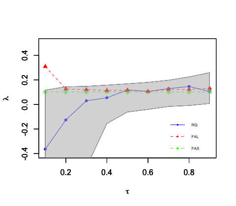


It is interesting that the constant estimators by FAL or FAS are almost constant separately on nine quantile levels in Figure but the estimators of traditional RQ method still vary. The second subfig show that estimators at nine quantiles by FAL only vary significantly from to , and not very significantly across all the nine quantile levels. To further verify the shrinkage results, we conduct hypothesis tests to check the constancy of slope coefficients. The Wald test for the equality of on quantile levels returns a -value of 0.01147, and on quantile levels returns a -value of 0.8663. The two -values imply the effect of spatial lag variables vary significantly across the all the nine quantile levels under significance level , but even nearly keep constant across . This agrees with the results from fused adaptive LASSO. For fused adaptive Lasso, the coefficients differences are penalized individually, so FAL could recognize the situation where the quantile slope coefficients appear constant in certain quantile regions, but vary in others.
On the other hand, for the covariate HOVAL and INC, the equality test on the quantile coefficients at returns two -values near zero, showing that at a whole the effect of HOVAL and INC vary across the nine quantile levels. The equality test at return -values 0.6438 and 0.2730 separately, which implying the effect of HOVAL and INC almost keep constant across . This is consist with the results by FAL. FAS method tends to shrink all the quantile coefficients to a constant so it couldn’t distinguish the single difference of the coefficients when between and .
6 Conclusion and discussion
In this paper, we suggest two new fused penalties methods (FAL and FAS) to shrinkage the interquantile parameters in spatial quantile autoregressive model. Through our method, we realized estimating the parameters and identifying the commonality among parameters in different quantiles at the same time. Lots of simulation experiments and real data analysis also show the greater performance of the new methods than that of traditional estimation method for spatial quantile autoregressive model.
In reality, however, there exist irrelevant variables. Most popular methods to select important predictors are also penalities approaches. How to combine the two penalization methods together in spatial quantile autoregressive model is an interesting research.
Appendix
A.1 Proof of Theorem 2.1
Proof.
Assumption (A1) - (A4) are the basic assmptions for SQAR model and make sure the existence of estimators.
In Assumption (A5), the sequence is independent and identically distributed, that is
Then
where is the th row vector of . Similarly, . So the sequence is independent and identically distributed. It is satisfied to the Assumption 1 in Kim and Muller 2004.
Denote the as the th element of , as the th column of of . Then
According to Assumption (A6), the second geometric moment of and the third geometric moment of are finite, so , that is the third geometric moment of is finite. The Assumption 2(i) in Kim and Muller 2004 is proved.
Under Assumption (A8),
where . According to Assumption (A8), and are finite and positive definite, so is also finite and positive definite. Similarly, is finite and positive definite. The Assumption 2(iii) in Kim and Muller 2004 is proved.
Under Assumption (A7) and (A9), the Assumption 2(ii) and 2(iv) are easily satisfied.
Thus, according to the Proposition 2 in Kim and Muller 2004, the Theorem 2.1 is proved. ∎
According to Jiang et. al. 2014, more general cases () have the similar propositions and theorems. So for ease to illustrate, we just consider in the next subsections.
A.2 Proof of Proposition 2.1
Proof.
Without loss of generality, we assume the quantile slopes vary for the first ( )quantiles, but remain constant for the remaining quantile levels.
At first, we consider about minimizing the following formula
The minimizer is and is a bounded vector. Under the identity in Knight 1998, we obtain
Then, can be written as
Denote we can rewrite as
According to the Assumptions (A10)-(A11), we need to show ’s mean and variance in detail.
It’s easy to see that for any fixed ,
Therefore, according to the Lindeberg-Feller Central Limit Theorem and Cramer-Wold Device, the first term and second of have,
where .
As for the third term , we know is a convex function and for any fixed .
Due to the Convexity Lemma in Jiang et. al. 2013, this pointwise convergence can be strengthened to the uniform convergence.
In other word, uniformly on any compact subset of .
In conclusion,
and the minimizer to , defined as , follows the asymptotic normal distribution , where
∎
A.3 Proof of Theorem 2.2
Without loss of generality, we consider the oracle estimator in the setting with . Then notation can then be simplified by letting be the th element of and for .
A.3.1 Root-n Consistency Lemma
Lemma 1 (Root-n consistency of ).
Assume conditions hold, if , then
Proof.
As in Fan and Li (2001), we only need to show that for any , there exists a sufficiently large constant , such that
where is defined in (2.16) when . In section 2.3.1, we assume the slopes vary for the first quantiles, but remain constant for the rest quantile levels. Then, we consider
| (A.1) | ||||
where for any . According to the assumption and , we have
uniformly in any compact set of .
Combined with the Proposition 2.1, the right side of inequality (A.1) is dominated by the quadratic term when is sufficiently large. Based on assumption (A11), we know is always holds when (as ).
∎
A.3.2 Proof of Theorem 2.2
Proof.
Sparsity:
Under the model assumption, can decomposed as , where , and . Denote and by the way of contradiction suppose . Let be a vector constructed by
replacing with in , that is, .We have
| (A.2) | ||||
Following the Lemma 1 of root-n consistent of , the first and the second term in (A.2) are both . Then, we consider the thrid term in
where , when . Therefore, (A.2) is dominated by the third term and always holds, which contradicts that is the minimizer of .
Asymptotic normality:
Let
| (A.3) | ||||
where is a fixed vector. According to the Proposition 2.1, we know
and
Therefore, the (A.3) can be deduced to the following conclusion.
and the minimizer to (A.3), defined as , follows the asymptotic normal distribution , where is the covariance matrix of the oracle estimator given in Proposition 2.1.
From the properties of convex functions, we know that the minimizer to (A.3) is unique and is a minimizer to (A.3). Hence, we get .
Jiang et. al. 2014 stated that more general cases follow the similar exposition, but with more complicated notations. So the Theorem 2.2 is proved.
∎
A.4 Proof of Proposition 2.2
Proof.
The proof is similar to the proof of Proposition 2.1 and thus is skipped. ∎
A.5 Proof of Theorem 2.3
Proof.
Similar to the proof of Theorem 2.2. ∎
A.5.1 Root-n Consistency Lemma
Lemma 2 (Root-n consistency of ).
Assume conditions hold, if , then
Proof.
As in Lemma 1, we only need to show that for any , there exists a sufficiently large constant , such that
where is defined in (2.17) in section . Note that
| (A.4) | ||||
where is the group-wise weight for the predictor and . Due to the assumption in section 2.3.2, we have
Combined with the Proposition 2.1, the right side of inequality (A.4) is dominated bu the quadratic term when n is sufficiently large. Based on assumption (A11), we know is also always holds when .
∎
A.5.2 Proof of Theorem 2.3
Proof.
Sparsity:
The proof is taken the similar arguments as theorem 2.1.
Under the assumption in section 2.3.2, can decomposed as , where and .
Denote and by the way of contradiction suppose .
Let be a vector constructed by replacing with in , that is,
.
Note that
| (A.5) | ||||
Following the Lemma 2 of , the first and second term in (A.5) are both . Similarly, the third term
where for , when . Therefore, (A.5) is dominated by the third term and always holds.
Asymptotic normality:
The proof is similar to the proof of Theorem 2.2 and thus is skipped.
∎
References
- (1)
- Akaike (1974) Akaike, H., (1974). A New Look at the Statistical Model Identification. IEEE Transactions on Aulomaic Control, 19(6), 716-723.
- Anselin and Bera (1998) Anselin, L., Bera, A. K. (1998). Spatial dependence in linear regression models with an introduction to spatial econometrics. Statistics textbooks and monographs, 155, 237-290.
- Anselin (2013) Anselin, L. (2013). Spatial econometrics: methods and models (Vol. 4). Springer Science and Business Media.
- Banerjee et al. (2003) Banerjee, S., Carlin, B. P., Gelfand, A. E. (2003). Hierarchical modeling and analysis for spatial data. Chapman and Hall/CRC.
- Barry and Pace (1999) Barry, R. P., Pace, R. K. (1999). Monte Carlo estimates of the log determinant of large sparse matrices. Linear Algebra and its applications, 289(1-3), 41-54.
- Bondell et al. (2010) Bondell, H. D., Reich, B. J., Wang, H. (2010). Noncrossing quantile regression curve estimation. Biometrika, 97(4), 825-838.
- Case (1991) Case, A. C. (1991). Spatial patterns in household demand. Econometrica: Journal of the Econometric Society, 953-965.
- Cliff and Ord (1973) Cliff, A.D., Ord, J.K., (1973). Spatial Autocorrelation. Pion Ltd., London.
- Ciuperca (2017) Ciuperca, G. (2017). Adaptive fused LASSO in grouped quantile regression. Journal of Statistical Theory and Practice, 11(1), 107-125.
- Fan and Li (2001) Fan, J., and Li, R., (2001). Variable Selection via Nonconcave Penalized Likelihood and Its Oracle Properties, Journal of the American statissical Association, 96, 1348-1360.
- Fan and Li (2004) Fan, J., Li, R. (2004). New estimation and model selection procedures for semiparametric modeling in longitudinal data analysis. Journal of the American Statistical Association, 99(467), 710-723.
- Friedman et. al. (2007) Friedman, J., Hastie, T., H’́ofling, H., Tibshirani, R. (2007). Pathwise coordinate optimization. The annals of applied statistics, 1(2), 302-332.
- Jiang et. al. (2013) Jiang, L., Wang, H. J., Bondell, H. D. (2013). Interquantile shrinkage in regression models. Journal of Computational and Graphical statistics, 22(4), 970-986.
- Jiang et. al. (2014) Jiang, L., Bondell, H. D., Wang, H. J. (2014). Interquantile shrinkage and variable selection in quantile regression. Computational Statistics and Data Analysis, 69, 208-219.
- He (1997) He, X., (1997). Quantile Curves Without Crossing. The American Statistician, 51, 186-192.
- Hoerl and Kennard (1970) Hoerl, A. E., Kennard, R. W. (1970). Ridge regression: Biased estimation for nonorthogonal problems. Technometrics, 12(1), 55-67.
- Huan et. al (2019) Huang, D., Lan, W., Zhang, H. H., Wang, H. (2019). Least squares estimation of spatial autoregressive models for large-scale social networks. Electronic Journal of Statistics, 13(1), 1135-1165.
- Kelejian and Prucha (2010) Kelejian, H. H., Prucha, I. R. (2010). Specification and estimation of spatial autoregressive models with autoregressive and heteroskedastic disturbances. Journal of econometrics, 157(1), 53-67.
- Kato (2010) Kato, K. (2010), Solving Regularization Problems With Piecewise Linear Losses, Journal of Computational and Graphical Statisics, 19, 1024-1040 .
- Kim and Muller (2004) Kim, T. H., Muller, C. (2004). Two-stage quantile regression when the first stage is based on quantile regression. The Econometrics Journal, 7(1), 218-231.
- Knight (1998) Knight, K. (1998). Limiting distributions for L1 regression estimators under general conditions. Annals of statistics, 755-770.
- Koenker and Bassett (1978) Koenker, R., Bassett Jr, G. (1978). Regression quantiles. Econometrica: journal of the Econometric Society, 33-50.
- Koenker (2005) Koenker, R., (2005). Quantile Regression. Cambridge University Press, Cambridge.
- Kostov (2013) Kostov, P. (2013). Empirical likelihood estimation of the spatial quantile regression. Journal of Geographical Systems, 15(1), 51-69.
- Lee (2003) Lee, L. F. (2003). Best spatial two-stage least squares estimators for a spatial autoregressive model with autoregressive disturbances. Econometric Reviews, 22(4), 307-335.
- LeSage (1999) LeSage, J. P., 1999. The theory and practice of spatial econometrics. www.spatial-econometrics.com.
- Liao and Wang (2012) Liao, W. C., Wang, X. (2012). Hedonic house prices and spatial quantile regression. Journal of Housing Economics, 21(1), 16-27.
- Liang and Li (2009) Liang, H., Li, R. (2009). Variable selection for partially linear models with measurement errors. Journal of the American Statistical Association, 104(485), 234-248.
- Lin and Lee (2010) Lin, X., Lee, L. F. (2010). GMM estimation of spatial autoregressive models with unknown heteroskedasticity. Journal of Econometrics, 157(1), 34-52.
- Liu et. al. (2018) Liu, X., Chen, J., Cheng, S. (2018). A penalized quasi-maximum likelihood method for variable selection in the spatial autoregressive model. Spatial statistics, 25, 86-104.
- Ma et. al. (2020) Ma, Y., Pan, R., Zou, T., Wang, H. (2020). A naive least squares method for spatial autoregression with covariates. Statistica Sinica, 30, 653-672.
- McMillen (2012) McMillen, D. P., (2012). Quantile regression for spatial data. Springer Science and Business Media.
- Pearl (2000) Pearl, J. (2000). Models, reasoning and inference. Cambridge, UK: Cambridge University Press, 19.
- Pollard (1991) Pollard, D. (1991). Asymptotics for least absolute deviation regression estimators. Econometric Theory, 7(2), 186-199.
- Rinaldo (2009) Rinaldo, A. (2009). Properties and refinements of the fused lasso. The Annals of Statistics, 37(5B), 2922-2952.
- Schwarz (1978) Schwarz, G. (1978). Estimating the dimension of a model. The annals of statistics, 461-464.
- Smirnov and Anselin (2001) Smirnov, O., Anselin, L. (2001). Fast maximum likelihood estimation of very large spatial autoregressive models: a characteristic polynomial approach. Computational Statistics and Data Analysis, 35(3), 301-319.
- Su and Yang (2011) Su, L., & Yang, Z. (2011). Instrumental Variable Quantile Estimation of Spatial Autoregressive Models.
- Tibshirani (1996) Tibshirani, R., (1996). Regression shrinkage and selection via the Lasso. Journal of the Royal Statistical Society, Series B 58, 267-288.
- Tibshirani et. al. (2005) Tibshirani, R., Saunders, M., Rosset, S., Zhu, J., and Knight, K. (2005), Sparsity and Smoothness via the Fused Lasso. Journal of the Royal Statistical Society, Series B, 67, 91-108.
- Trefethen and Bau (1997) Trefethen, L. N., Bau III, D. (1997). Numerical linear algebra (Vol. 50). Siam.
- Wright (1928) Wright, P. G. (1928). Tariff on animal and vegetable oils. Macmillan Company, New York.
- Xie et. al. (2020) Xie, T., Cao, R., Du, J. (2020). Variable selection for spatial autoregressive models with a diverging number of parameters. Statistical Papers, 61(3), 1125-1145.
- Xu and Lee (2015) Xu, X., Lee, L. F. (2015). A spatial autoregressive model with a nonlinear transformation of the dependent variable. Journal of Econometrics, 186(1), 1-18.
- Yuan and Lin (2006) Yuan, M., Lin, Y., (2006). Model Selection and Estimation in Regression With Grouped Variables. Journal of the Royal Statisical Society, Series B, 68, 49-67.
- Zhao et. al. (2006) Zhao, P., Rocha, G., Yu, B. (2009). The composite absolute penalties family for grouped and hierarchical variable selection. The Annals of Statistics, 37(6A), 3468-3497.
- Zhang and Shen (2015) Zhang Y. Q., Shen D. M., (2015). Estimation of semi-parametric varying-coefficient spatial panel data models with random-effects. Journal Statistical Plan and Inference 159:64-80
- Zhang and Xiang (2015) Zhang, C., Xiang, Y., 2015. On the oracle property of adaptive group LASSO in high-dimensional linear models. Statistical Papers, 57(1), 249-265.
- Zietz et. al. (2008) Zietz, J., Zietz, E. N., Sirmans, G. S. (2008). Determinants of house prices: a quantile regression approach. The Journal of Real Estate Finance and Economics, 37(4), 317-333.
- Zou (2006) Zou, H., (2006), The Adaptive Lasso and Its Oracle Properties. Journal of the American Satistical Association, 101, 1418-1429.
- Zou and Yuan (2008a) Zou, H., Yuan, M., 2008a. Composite quantile regression and the oracle model selection theory. The Annals of Statistics 36, 1108-1126.
- Zou and Yuan (2008b) Zou, H., Yuan, M., 2008b. Regularized simultaneous model selection in multiple quantiles regression. Computational Statistics and Data Analysis 52, 5296-5304.