跳到论文正文
W Papers独立论文阅读器 arXiv:2111.06960 论文正文 计算阅读时间 · 0%
引用这篇论文根据当前论文元数据生成,正式投稿前建议核对。


License: arXiv.org perpetual non-exclusive license
arXiv:2111.06960v1 [math.PR] 12 Nov 2021

A new proof of reversibility of S​L​EκSLE_{\kappa} for κ≤4\kappa\leq 4

Gregory F. Lawler Thanks: Research supported by National Science Foundation grant DMS-1513036    Stephen Yearwood Affiliation: Department of Mathematics Affiliation: University of Chicago
Abstract

We give a new proof of the reversibility of the Schramm Loewner evolution for κ≤4\kappa\leq 4. The main ideas used in the proof are similar to those used in the original proof of this result, given by Zhan.

1 Introduction

The Schramm Loewner evolution (S​L​EκSLE_{\kappa}) is a one parameter family of probability measures on curves in the plane parametrized by κ=2/a>0\kappa=2/a>0. It gives the only candidate for scaling limits of discrete lattice models exhibiting conformal invariance in the continuum limit. We recall the definition; see [2] for more detail. Let ℍ{\mathbb{H}} denote the upper half plane in ℂ{\mathbb{C}}. If γ:[0,∞)→ℍ¯\gamma:[0,\infty)\rightarrow\overline{{\mathbb{H}}} is a curve, we write γt\gamma_{t} for γ⁡[0,t]\gamma[0,t] and DtD_{t} for the unbounded component of ℍ∖γt{\mathbb{H}}\setminus\gamma_{t}. Chordal S​L​EκSLE_{\kappa} from 00 to ∞\infty is defined (up to a choice of parametrization) as a random curve γ:[0,∞)→ℍ\gamma\colon[0,\infty)\to{\mathbb{H}} with γ⁡(0)=0\gamma(0)=0 such that the following holds. Let gtg_{t} be the “mapping-out function”, that is, the unique conformal transformation gt:Dt→ℍg_{t}:D_{t}\rightarrow{\mathbb{H}} with gt​(z)=z+o⁡(1)g_{t}(z)=z+o(1) as z→∞z\rightarrow\infty. Then gtg_{t} satisfies

g˙t​(z)=agt​(z)−Utg0​(z)=z\dot{g}_{t}(z)=\frac{a}{g_{t}(z)-U_{t}}\qquad g_{0}(z)=z (1)

Under this parameterization, hcap⁡(γt)=a​t{\rm hcap}(\gamma_{t})=at, where hcap{\rm hcap} denotes the half-plane capacity. In other words, we have the expansion

gt​(z)=z+a​tz+O⁡(|z|−2),z→∞.g_{t}(z)=z+\frac{at}{z}+O(|z|^{-2}),\;\;\;\;z\rightarrow\infty.

If z∈ℂ∖0z\in\mathbb{C}\setminus 0, the solution to (1) holds for all t<Tzt<T_{z} where

Tz=sup𝑡{min{|gs(z)−Us|:0≤s≤t}>0}.T_{z}=\underset{t}{\text{sup}}\{\text{min}\{|g_{s}(z)-U_{s}|:0\leq s\leq t\}>0\}.

To get chordal S​L​EκSLE_{\kappa} connecting distinct boundary points in a simply connected domain DD, one takes the conformal image of this under a conformal map. Again this is defined up to a change of parametrizaton.

While S​L​ESLE is a model for curves in equilibrium, the definition uses conditional probabilities given the path up to a certain time and hence adds an artificial dynamic. One disadvantage is that some properties that are expected of the limit curve, in particular reversibility, do not follow immediately. Zhan showed this to be true [6] for κ≤4\kappa\leq 4, while Miller and Sheffield were able to extend these results to κ∈(0,8)\kappa\in(0,8) [3, 4, 5] by realizing S​L​EκSLE_{\kappa} curves as flow lines of the Gaussian free field.

The purpose of this note is to give a new proof of reversibility for κ≤4\kappa\leq 4; we hope in future work to extend this to 4<κ<84<\kappa<8 to give a proof that does not make use of the tools of the Gaussian free field. While we say that it is a new proof, the basic idea of the proof is the same as that given by Zhan. Our hope is that we our argument simplifies some of the details. We write S​L​ESLE for S​L​EκSLE_{\kappa}.

  • •

    We compare S​L​ESLE from 00 to xx in ℍ{\mathbb{H}} to S​L​ESLE from xx to 00. These are probability measures on bounded curves γ\gamma with hcap⁡(γ)<∞{\rm hcap}(\gamma)<\infty. While hcap⁡(γ){\rm hcap}(\gamma) is a random quantity, it is almost immediate from the definition that the distribution of hcap⁡(γ){\rm hcap}(\gamma) is the same for S​L​ESLE in both directions.

  • •

    We view S​L​ESLE connecting two points in ℝ{\mathbb{R}} as a probability measure on the final mapping-out functions gγg_{\gamma}.

  • •

    We then focus on S​L​ESLE from 00 to xx and xx to 00 conditioned to have a specific half-plane capacity. We show that these two probability measures agree on the conformal maps gγg_{\gamma} for each value of hcap⁡[γ]{\rm hcap}[\gamma]. By scaling it suffices to prove this for all xx assuming hcap⁡[γ]=a{\rm hcap}[\gamma]=a.

  • •

    For each r∈[0,1]r\in[0,1] we consider the probability measure μr\mu_{r} which corresponds to the following:

    • –

      Take S​L​ESLE from 00 to xx conditioned to have hcap=a{\rm hcap}=a stopped at time rr, that is, when hcap=r​a{\rm hcap}=ra giving γ1\gamma^{1}.

    • –

      Given γ1\gamma^{1}, let γ2\gamma^{2} be S​L​ESLE from xx to γ1​(r)\gamma^{1}(r) in ℍ∖γ1{\mathbb{H}}\setminus\gamma^{1} conditioned so that hcap⁡(γ1∪γ2)=a{\rm hcap}(\gamma^{1}\cup\gamma^{2})=a.

    • –

      Output gγg_{\gamma} where γ=γ1⊕γ~\gamma=\gamma^{1}\oplus\tilde{\gamma} where γ~\tilde{\gamma} is the reversal of γ2\gamma^{2}.

    This gives a probability measure on transformations gγg_{\gamma} with hcap⁡[γ]=a{\rm hcap}[\gamma]=a which we denote by μr\mu_{r}.

  • •

    We consider this as a measure on continuous functions on a fixed closed ball K=Kh⊂ℍK=K_{h}\subset{\mathbb{H}} where hh is large enough so that Im⁡[gγ​(z)]≥a{\rm Im}[g_{\gamma}(z)]\geq a for all z∈Kz\in K and hcap⁡[γ]=a{\rm hcap}[\gamma]=a. We show that the Prokhorov distance between μr\mu_{r} and μs\mu_{s} is less than c​|s−r|1+δc|s-r|^{1+\delta} for some δ>0\delta>0. We conclude that μs\mu_{s} is a constant function of ss. In particular, μ0=μ1\mu_{0}=\mu_{1} which is the main result.

  • •

    The main local commutation relation which is similar to the relations in [6] and [1] is expressed in terms of Radon-Nikodym derivatives of independent S​L​ESLE paths tilted by a Brownian loop term. This relation is nicest for κ≤4\kappa\leq 4, but we discuss the κ<8\kappa<8 case here in order to prepare for future work.

The paper is organized as follows. In Section 2, we review S​L​ESLE connecting two points on the boundary, together with some other basic notation, and then we state the main theorem of this paper. In Section 3, we describe the commutation relation, and show explicitly that the measures under consideration have the same Radon-Nikodym derivative with respect to a particular measure. In Section 4 we prove the main theorem in a sequence of steps, relying on a few Loewner chain estimates. Finally, in Section 5, we give the (delayed) proof of a basic Bessel process fact.

Throughout this paper we fix κ=2/a∈(0,8)\kappa=2/a\in(0,8) and allow constants, both implicit and explicit, to depend on κ\kappa. We write just S​L​ESLE for S​L​EκSLE_{\kappa}. For a number of the results, we need κ≤4\kappa\leq 4 and we say that. Let

b=6−κ2​κ=3​a−12b=\frac{6-\kappa}{2\kappa}=\frac{3a-1}{2}

be the boundary scaling exponent.

2 S​L​ESLE in ℍ{\mathbb{H}} from x1x_{1} to x2x_{2}

There are several equivalent characterizations of S​L​ESLE connecting two real points; here we will take the perspective of S​L​ESLE from 00 to x∈ℝ∖{0}x\in{\mathbb{R}}\setminus\{0\} as S​L​ESLE from 00 to ∞\infty in ℍ{\mathbb{H}} tilted by the partition function Ψ\Psi. For simply connected domains and locally analytic boundary points z,wz,w, the partition function for S​L​ESLE is ΨD​(z,w)=H∂D​(z,w)b\Psi_{D}(z,w)=H_{\partial D}(z,w)^{b}. Here H∂D​(z,w)H_{\partial D}(z,w) is the boundary Poisson kernel normalized so that Hℍ​(0,x)=x−2H_{\mathbb{H}}(0,x)=x^{-2}. We also define Ψℍ​(x,∞)=1\Psi_{\mathbb{H}}(x,\infty)=1 for all x∈ℍx\in{\mathbb{H}}. The partition function satisfies the scaling rule: if f:D→f⁡(D)f:D\rightarrow f(D) is a conformal transformation, then

ΨD​(z,w)=|f′​(z)|b​|f′​(w)|b​Ψf⁡(D)​(f⁡(z),f⁡(w)).\Psi_{D}(z,w)=|f^{\prime}(z)|^{b}\,|f^{\prime}(w)|^{b}\,\Psi_{f(D)}(f(z),f(w)).

Although this definition of ΨD​(z,w)\Psi_{D}(z,w) requires that z,wz,w be locally analytic boundary points, ratios of partition functions can often be defined using the scaling rule as we will see below.

Suppose that gtg_{t} satisfies (1) where Ut=−BtU_{t}=-B_{t} is a standard Brownian motion defined on a probability space (Ω,ℱ,ℙ)(\Omega,{\mathcal{F}},{\mathbb{P}}). Let γ⁡(t)\gamma(t) denote the corresponding S​L​EκSLE_{\kappa} curve and we write γt=γ(0,t]\gamma_{t}=\gamma(0,t]. Under the measure ℙ{\mathbb{P}}, γ\gamma has the distribution of an S​L​EκSLE_{\kappa} path from 00 to ∞\infty. We will tilt the measure ℙ{\mathbb{P}} using an appropriate local martingale to get S​L​ESLE from 00 to xx. Suppose x∈ℝ∖{0}x\in{\mathbb{R}}\setminus\{0\}, and let Xt=gt​(x)−UtX_{t}=g_{t}(x)-U_{t} and T=Tx=inf{t>0:Xt=0}T=T_{x}=\inf\{t>0:X_{t}=0\}. For t<Tt<T, let DtD_{t} be the unbounded component of ℍ∖γt{\mathbb{H}}\setminus\gamma_{t}, and define the local martingale MtM_{t} formally by

Mt=x1−3​a​ΨHt​(γ​(t),x)ΨDt​(γ​(t),∞),t<T.M_{t}=x^{1-3a}\dfrac{\Psi_{H_{t}}(\gamma(t),x)}{\Psi_{D_{t}}(\gamma(t),\infty)},\qquad t<T.

The partition functions on the right-hand side are not well defined but the ratio is well defined using the scaling rule,

ΨDt​(γ​(t),x)ΨDt​(γ​(t),∞)=|g′​(γt)|b​g′​(x)b​ΨDt​(Ut,gt​(x))|g′​(γt)|b​g′​(∞)​Ψℍ​(Ut,∞)=gt′​(x)b​Xt1−3​a.\dfrac{\Psi_{D_{t}}(\gamma(t),x)}{\Psi_{D_{t}}(\gamma(t),\infty)}=\dfrac{\left|g^{\prime}(\gamma_{t})\right|^{b}\,g^{\prime}(x)^{b}\,\Psi_{D_{t}}(U_{t},g_{t}(x))}{\left|g^{\prime}(\gamma_{t})\right|^{b}\,g^{\prime}(\infty)\,\Psi_{{\mathbb{H}}}(U_{t},\infty)}=g^{\prime}_{t}(x)^{b}X_{t}^{1-3a}.

While this is formal, this shows that we can define

Mt=(XtX0)1−3​a​gt′​(x)b,t<TM_{t}=\left(\frac{X_{t}}{X_{0}}\right)^{1-3a}\,g_{t}^{\prime}(x)^{b},\;\;\;\;t<T

and one can use Itô’s formula and the Loewner equation to see that MtM_{t} is a local martingale satisfying M0=1M_{0}=1 and

d​Mt=1−3​aXt​Mt​d​Bt,    0≤t<T.dM_{t}=\frac{1-3a}{X_{t}}\,M_{t}\,dB_{t},\;\;\;\;0\leq t<T. (2)

Let ℙ∗{\mathbb{P}}^{*} be the measure obtained by tilting by MtM_{t}. More precisely, if τ<T\tau<T is a stopping time such that Mt∧τM_{t\wedge\tau} is a martingale and VV is an event measurable with respect to ℱt∧τ{\mathcal{F}}_{t\wedge\tau}, then ℙ∗​(V)=𝔼⁡[Mt∧τ​ 1V]{\mathbb{P}}^{*}(V)={\mathbb{E}}[M_{t\wedge\tau}\,1_{V}]. The Girsanov theorem states that

d​Bt=1−3​aXt​d​t+d​Wt,    0≤t<T,dB_{t}=\frac{1-3a}{X_{t}}\,dt+dW_{t},\;\;\;\;0\leq t<T,

where WtW_{t} is a standard Brownian motion with respect to ℙ∗{\mathbb{P}}^{*} and hence

d​Xt=1−2​aXt​d​t+d​Wt,    0≤t<T.dX_{t}=\frac{1-2a}{X_{t}}\,dt+dW_{t},\;\;\;\;0\leq t<T.

The following is well known.

Proposition 2.1.

Suppose 0<x0<x and gtg_{t} is the solution to the Loewner equation (1) where Ut=gt​(x)−XtU_{t}=g_{t}(x)-X_{t} and XtX_{t} satisfies

d​Xt=1−2​aXt​d​t+d​Wt,X0=x,    0≤t<T,dX_{t}=\frac{1-2a}{X_{t}}\,dt+dW_{t},\;\;\;X_{0}=x,\;\;\;\;0\leq t<T, (3)

where WtW_{t} is a standard Brownian motion and T=inf{t:Xt=0}T=\inf\{t:X_{t}=0\}. Then γ⁡(t),0≤t≤T\gamma(t),0\leq t\leq T has the distribution of S​L​EκSLE_{\kappa} from 00 to xx parametrized by half plane capacity from infinity stopped at the time that γT\gamma_{T} disconnects xx from infinity. In particular, hcap⁡[γT]=a​T{\rm hcap}[\gamma_{T}]=aT.

Indeed to verify this, one needs only check that the conformal image of S​L​ESLE from 00 to ∞\infty by a conformal transformation F:ℍ→ℍF:{\mathbb{H}}\rightarrow{\mathbb{H}} with F⁡(0)=0,F⁡(∞)=xF(0)=0,F(\infty)=x gives the same distribution on the driving function as (3).

Similarly, if XtX_{t} satisfies (3) and we define U~t=gt​(0)−Xt\tilde{U}_{t}=g_{t}(0)-X_{t} with corresponding curve γ~\tilde{\gamma}, then γ~​(t),0≤t≤T\tilde{\gamma}(t),0\leq t\leq T has the distribution of S​L​EκSLE_{\kappa} from xx to 00 parametrized by half plane capacity from infinity stopped at the time that γT\gamma_{T} disconnects 00 from infinity.

While we may use the same XtX_{t} for S​L​ESLE in both directions, the distribution of the driving functions Ut,U~tU_{t},\tilde{U}_{t} are different. Indeed, U0=x,U~0=0U_{0}=x,\tilde{U}_{0}=0. For this reason, we cannot conclude the reversibility immediately from this fact. One thing that does follow is that the distribution of the stopping time TT is the same for S​L​ESLE from 00 to xx as for S​L​ESLE from xx to 00. It is the same as the time to reach the origin for the Bessel process (3). Since a>1/4a>1/4 the process reaches the origin in finite time.

There is a significant difference between κ∈(0,4]\kappa\in(0,4] and κ∈(4,8)\kappa\in(4,8). Let us consider S​L​ESLE from 00 to xx with x>0x>0 stopped at time TT. The following statements are with probability one with respect to the tilted measure ℙ∗{\mathbb{P}}^{*}.

  • •

    If 0<κ≤40<\kappa\leq 4, then γ⁡(t),0≤t≤T\gamma(t),0\leq t\leq T is a simple curve with γ⁡(0)=0,γ⁡(T)=x,γ⁡(0,T)⊂ℍ\gamma(0)=0,\gamma(T)=x,\gamma(0,T)\subset{\mathbb{H}}.

  • •

    If 4<κ<84<\kappa<8, then γ⁡(T)∈(x,∞)\gamma(T)\in(x,\infty). Although the S​L​ESLE curve continues after time TT, D∞D_{\infty}, the unbounded connected component of ℍ∖γ{\mathbb{H}}\setminus\gamma is the same as the unbounded connected component of ℍ∖γT{\mathbb{H}}\setminus\gamma_{T}.

In particular, for κ≤4\kappa\leq 4, the domain D∞D_{\infty} determines the entire curve while for 4<κ<84<\kappa<8, the domain D∞D_{\infty} gives only the “curve as viewed from infinity”, that is γ∩D¯∞\gamma\cap\overline{D}_{\infty}. We will prove reversibility for the domain D∞D_{\infty}. In this paper, we do the κ≤4\kappa\leq 4 case reproving Zhan’s result.

Theorem 1.

If κ≤4\kappa\leq 4, the distribution of D∞D_{\infty}, is the same for S​L​ESLE from x1x_{1} to x2x_{2} and for S​L​ESLE from x2x_{2} to x1x_{1}. Equivalently, the distribution of the conformal transformation g∞g_{\infty} is the same.

Our proof is in the same spirit as Zhan’s proof. One novel aspect is that we choose a realization of the Bessel process (3) in a two step process: we first choose a value T=t0T=t_{0} and then given TT we run the Bessel process conditioned so that T=t0T=t_{0}.

If XtX_{t} satisfies (3) where WtW_{t} is a ℙ∗{\mathbb{P}}^{*}-Brownian motion, then the transition probability of the process killed at the origin is

qs​(x,y)=yx4​a+1​s2​a+12​exp⁡{−x2+y22​s}​h​(x​ys),q_{s}(x,y)=\frac{y}{x^{4a+1}\,s^{2a+\frac{1}{2}}}\,\exp\left\{-\frac{x^{2}+y^{2}}{2s}\right\}\,h\left(\frac{xy}{s}\right),

where h=hah=h_{a} is an entire function with h⁡(0)>0h(0)>0. The density of TT in the measure ℙ∗{\mathbb{P}}^{*} is a constant times

ϕ⁡(x,t):=x4​a−1​t−12−2​a​exp⁡{−x22​t}.\phi(x,t):=x^{4a-1}\,t^{-\frac{1}{2}-2a}\,\exp\left\{-\frac{x^{2}}{2t}\right\}. (4)

The Bessel process conditioned so that T=t0T=t_{0} is this process tilted by the ℙ∗{\mathbb{P}}^{*}-martingale

Nt:=ϕ⁡(Xt,t0−t),0≤t<t0N_{t}:=\phi(X_{t},t_{0}-t),\qquad 0\leq t<t_{0} (5)

which satisfies

d​Nt=Nt​[4​a−1Xt−Xtt0−t]​d​Wt.dN_{t}=N_{t}\left[\frac{4a-1}{X_{t}}-\frac{X_{t}}{t_{0}-t}\right]\,dW_{t}. (6)

Formally one can write ϕ⁡(Xt,t0−t)=𝔼∗​[𝟙T=t0|Xt]\phi(X_{t},t_{0}-t)={\mathbb{E}}^{*}[\mathbbm{1}_{T=t_{0}}|X_{t}] which can be thought of as a Doob martingale in the measure ℙ∗{\mathbb{P}}^{*}. Otherwise, the unconvinced reader may engage in a brief Itô calculus exercise to derive (6). Since MtM_{t} is a ℙ{\mathbb{P}} local martingale and NtN_{t} is a ℙ∗{\mathbb{P}}^{*} local martingale, we can see that M~t:=Mt​Nt\tilde{M}_{t}:=M_{t}\,N_{t} is a ℙ{\mathbb{P}} local martingale. Again, one can check this again using Itô calculus. If we let

M~t=M~t,t0=Mt​Nt=x1−3​a​Xt3​a−1​gt′​(x)(3​a−1)/2​ϕ​(Xt,t0−t),   0≤t<t0,\tilde{M}_{t}=\tilde{M}_{t,t_{0}}=M_{t}\,N_{t}=x^{1-3a}\,X_{t}^{3a-1}\,g_{t}^{\prime}(x)^{(3a-1)/2}\,\phi(X_{t},t_{0}-t),\;\;\;0\leq t<t_{0},

then using (2) and (5) we see that M~t,0≤t<t0\tilde{M}_{t},0\leq t<t_{0} is a ℙ{\mathbb{P}}-martingale satisfying

d​M~t=[aXt−Xtt0−t]​M~t​d​Bt,0≤t<t0.d\tilde{M}_{t}=\left[\frac{a}{X_{t}}-\frac{X_{t}}{t_{0}-t}\right]\,\tilde{M}_{t}\,dB_{t},\qquad 0\leq t<t_{0}.

If we tilt in the Girsanov sense as above by M~t\tilde{M}_{t} giving the new measure ℙ^\hat{{\mathbb{P}}} we have

d​Bt=[aXt−Xtt0−t]​d​t+d​W~t,dB_{t}=\left[\frac{a}{X_{t}}-\frac{X_{t}}{t_{0}-t}\right]\,dt+d\tilde{W}_{t},
d​Xt=d⁡[gt​(x)+Bt]=[2​aXt−Xtt0−t]​d​t+d​W~t,dX_{t}=d[g_{t}(x)+B_{t}]=\left[\frac{2a}{X_{t}}-\frac{X_{t}}{t_{0}-t}\right]\,dt+d\tilde{W}_{t},

where W~t\tilde{W}_{t} is a ℙ~\tilde{{\mathbb{P}}}-Brownian motion.

Suppose x1,x2x_{1},x_{2} are distinct real numbers, 0<κ<80<\kappa<8, and 0<t0<∞0<t_{0}<\infty. Then S​L​EκSLE_{\kappa} from x1x_{1} to x2x_{2} in ℍ{\mathbb{H}} of time duration t0t_{0} is defined to be the solution of (1) where the driving function Ut=gt​(x2)−XtU_{t}=g_{t}(x_{2})-X_{t}, and XtX_{t} satisfies

d​Xt=[2​aXt−Xtt0−t]​d​t+d​Wt,X0=x2−x1,dX_{t}=\left[\frac{2a}{X_{t}}-\frac{X_{t}}{t_{0}-t}\right]\,dt+dW_{t},\;\;\;\;X_{0}=x_{2}-x_{1}, (7)
Ut=gt​(x2)−Xt=x2+∫0ta​d​sXs−Xt,U_{t}=g_{t}(x_{2})-X_{t}=x_{2}+\int_{0}^{t}\frac{a\,ds}{X_{s}}-X_{t},

where WtW_{t} is a standard Brownian motion.

If qt​(x,y)q_{t}(x,y) denotes the transition probability for a Bessel process satisfying (3), killed upon reaching the origin, then the density for a process satisfying (7) is

ψt​(x,y,t0)=qt​(x,y)​ϕ⁡(y,t0−t)ϕ⁡(x,t0).\psi_{t}(x,y;t_{0})=q_{t}(x,y)\,\frac{\phi(y,t_{0}-t)}{\phi(x,t_{0})}.

We will need one very believable fact about this process. The proof uses standard techniques but we delay the proof to Section 5. This estimate is not optimal but will be more than sufficient for our purposes.

Proposition 2.2.

For every 0<κ<80<\kappa<8, there exists c​<∞,u>​0c<\infty,u>0 such that if XtX_{t} satisfies (7), then for all r>0r>0,

ℙ{max0≤t≤t0|Ut−x1|≥t0(|x2−x1|+r2)}≤ce−u​r.{\mathbb{P}}\left\{\max_{0\leq t\leq t_{0}}|U_{t}-x_{1}|\geq\sqrt{t_{0}}\,(|x_{2}-x_{1}|+r^{2})\right\}\leq c\,e^{-ur}.

We denote the corresponding probability measure on paths (modulo reparametrization) by μ#​(x1,x2,t0)\mu^{\#}(x_{1},x_{2};t_{0}). Assuming x1<x2x_{1}<x_{2}, we have the following:

  • •

    γ⁡(0)=x1\gamma(0)=x_{1}, T=t0T=t_{0};

  • •

    hcap⁡[γt]=a​t, 0≤t≤T{\rm hcap}[\gamma_{t}]=at,\;0\leq t\leq T;

  • •

    If κ≤4\kappa\leq 4, then γT\gamma_{T} is a simple curve with γ⁡(0,t0)⊂ℍ\gamma(0,t_{0})\subset{\mathbb{H}} and γ⁡(t0)=x2\gamma(t_{0})=x_{2}. Moreover, ∂D∞∩ℍ=γ⁡(0,t0)\partial D_{\infty}\cap{\mathbb{H}}=\gamma(0,t_{0});

  • •

    If 4<κ<84<\kappa<8, then

    γ⁡(T)=x+:=max⁡{y∈ℝ:y∈γt0}>x2,\gamma(T)=x_{+}:=\max\{y\in{\mathbb{R}}:y\in\gamma_{t_{0}}\}>x_{2},
    x−:=min⁡{y∈ℝ:y∈γt0}<x1.x_{-}:=\min\{y\in{\mathbb{R}}:y\in\gamma_{t_{0}}\}<x_{1}.

    Indeed, ∂D∞∩ℍ\partial D_{\infty}\cap{\mathbb{H}} is a curve connecting x−x_{-} to x+x_{+}.

To prove Theorem 1 it suffices to prove the following.

Theorem 2.

If κ≤4\kappa\leq 4 then for every t0>0t_{0}>0 and x1<x2x_{1}<x_{2}, the measure μ#​(x1,x2,t0)\mu^{\#}(x_{1},x_{2};t_{0}) is the same as μ#​(x2,x1,t0)\mu^{\#}(x_{2},x_{1};t_{0}) if considered as probability measures on the conformal transformation g=gt0g=g_{t_{0}}.

By scaling and translation invariance it suffices to prove this with x1=0,x2=x>0x_{1}=0,x_{2}=x>0 and t0=1t_{0}=1.

Fix x>0x>0 and consider the measure μr=μr,x\mu_{r}=\mu_{r,x}, 0≤r≤10\leq r\leq 1 obtained as follows:

  • •

    Grow the curve γ\gamma under the measure μ#​(0,x,1)\mu^{\#}(0,x;1) until time rr giving curve γr\gamma_{r} and corresponding map grg_{r}. Let z1=gr​(γ⁡(r)),w1=gr​(1)z_{1}=g_{r}(\gamma(r)),w_{1}=g_{r}(1).

  • •

    Given γr\gamma_{r}, let γ~\tilde{\gamma} be S​L​ESLE from xx to γ⁡(r)\gamma(r) in ℍ∖γr{\mathbb{H}}\setminus\gamma_{r} conditioned so that hcap​[γr∪γ~]=a\text{hcap}[\gamma_{r}\cup\tilde{\gamma}]=a. Equivalently, let η\eta be chosen from μ#​(w1,z1,1−r)\mu^{\#}(w_{1},z_{1};1-r) and let γ~=gr−1∘η\tilde{\gamma}=g_{r}^{-1}\circ\eta. Let h=gηh=g_{\eta} and g=h∘grg=h\circ g_{r}.

Note that μ0=μ#​(0,x,1),μ1=μ#​(x,0,1)\mu_{0}=\mu^{\#}(0,x;1),\mu_{1}=\mu^{\#}(x,0;1). We will prove the following stronger result,

Proposition 2.3.

If κ≤4\kappa\leq 4 and x>0x>0, then for all 0≤r≤10\leq r\leq 1, μr=μ0\mu_{r}=\mu_{0}.

Since hcap⁡[γ1]=a{\rm hcap}[\gamma_{1}]=a, we know that γ1⊂{z:Im​(z)2≤2​a}\gamma_{1}\subset\{z:{\rm Im}(z)^{2}\leq{2a}\} and hence with probability one for each μr\mu_{r}, D∞⊃{z:Im​(z)2>2​a}D_{\infty}\supset\{z:{\rm Im}(z)^{2}>{2a}\}. Let ℐ={z:|z−(8​a+1)​i|≤1}\mathcal{I}=\{z:|z-(\sqrt{8a}+1)i|\leq 1\}. Let SS denote the set of continuous functions from ℐ{\mathcal{I}} to ℂ{\mathbb{C}} endowed with the supremum norm ∥⋅∥\|\cdot\|. We also write ρ\rho for the corresponding Prokhorov metric on probability measures on SS. Since the conformal map gg is determined by its values on ℐ{\mathcal{I}}, it suffices to prove that for every ϵ>0\epsilon>0 and 0≤r<s≤10\leq r<s\leq 1, ρ⁡(μr,μs)<ϵ\rho(\mu_{r},\mu_{s})<\epsilon. We will show the following.

Proposition 2.4.

For every K<∞K<\infty, there exists c,δc,\delta such that if 0<x≤K0<x\leq K and 0≤r≤s≤10\leq r\leq s\leq 1, we can couple (g,g~)(g,\tilde{g}) on the same probability space such that gg has distribution μr\mu_{r}, g~\tilde{g} has distribution μs\mu_{s} and

ℙ{∥g−g~∥≥c(s−r)1+δ}≤c(s−r)δ,{\mathbb{P}}\{\|g-\tilde{g}\|\geq c\,(s-r)^{1+\delta}\}\leq c\,(s-r)^{\delta},
ℙ{∥g−g~∥≥c(s−r)}≤c(s−r)1+δ.{\mathbb{P}}\{\|g-\tilde{g}\|\geq c\,(s-r)\}\leq c\,(s-r)^{1+\delta}.

We state it this way in preparation for later work in the 4<κ<84<\kappa<8 case. For 0<κ≤40<\kappa\leq 4, we do significantly better by giving a coupling that satisfies ‖g−g~‖≤c⁡(s−r)\|g-\tilde{g}\|\leq c\,(s-r) for all (g,g~)(g,\tilde{g}) and such that ℙ{∥g−g~∥≥(s−r)5/4}{\mathbb{P}}\{\|g-\tilde{g}\|\geq(s-r)^{5/4}\} decays faster than every power of s−rs-r.

Note that Proposition 2.4 implies that there exist c,δc,\delta

ρ⁡(μr,μs)≤c​(s−r)1+δ.\rho(\mu_{r},\mu_{s})\leq c\,(s-r)^{1+\delta}.

This shows that μr\mu_{r} is Hölder continuous of order 1+δ1+\delta in rr and a standard argument shows that this means that μr\mu_{r} is a constant function of rr and hence Proposition 2.3 holds.

3 Local commutation relation

In this section we will state the basic “commutation” relation that we will use. In order to state the relation precisely we will set up some notation. Although we only use it for κ≤4\kappa\leq 4 in this paper, we will also give a result that holds for all 4<κ<84<\kappa<8. We fix x1≠x2x_{1}\neq x_{2} and t0>0t_{0}>0. Suppose γ:[0,t0]→ℍ\gamma:[0,t_{0}]\rightarrow{\mathbb{H}} is a non-crossing curve parametrized by capacity from x1x_{1} to x2x_{2} in ℍ{\mathbb{H}}. Let γ^R\hat{\gamma}^{R} denote the reversed curve from x2x_{2} to x1x_{1} defined by γ^R​(t)=γ⁡(t0−t), 0≤t≤t0\hat{\gamma}^{R}(t)=\gamma(t_{0}-t),\;0\leq t\leq t_{0}. Although γ^R\hat{\gamma}^{R} is not parametrized by capacity, we can reparametrize it γR​(t)=γ^R​(σ⁡(t))\gamma^{R}(t)=\hat{\gamma}^{R}(\sigma(t)) so that for each tt, hcap⁡[γtR]=a​t{\rm hcap}[\gamma^{R}_{t}]=at. The total time duration of γR\gamma^{R} is the same as that of γ\gamma, t0t_{0}.

If 0<s1<s2<t00<s_{1}<s_{2}<t_{0}, we can write

γ=γs1⊕γ⁡[s1,s2]⊕γ⁡[s2,t0],\gamma=\gamma_{s_{1}}\oplus\gamma[s_{1},s_{2}]\oplus\gamma[s_{2},t_{0}],

Let us write γ1\gamma^{1} for γs1\gamma_{s_{1}} and γ2\gamma^{2} for the reversal of γ⁡[s2,t0]\gamma[s_{2},t_{0}], so that we have

γ=γ1⊕η⊕(γ2)R.\gamma=\gamma^{1}\oplus\eta\oplus(\gamma^{2})^{R}. (8)

Let us view this at the moment as a decomposition modulo reparametrization but still remember that hcap⁡[γ]=a​t0{\rm hcap}[\gamma]=at_{0} and we assume that

hcap⁡[γ1∪(γ2)R]=hcap⁡[γ1∪γ2]<a​t0.{\rm hcap}[\gamma^{1}\cup(\gamma^{2})^{R}]={\rm hcap}[\gamma^{1}\cup\gamma^{2}]<at_{0}.

We will also assume that

γ1∩γ2=∅.\gamma^{1}\cap\gamma^{2}=\emptyset.

If κ≤4\kappa\leq 4, this will happen with probability one since S​L​EκSLE_{\kappa} is supported on simple curves, but for κ>4\kappa>4 this is a nontrivial constraint.

Suppose r1+r2≤t0r_{1}+r_{2}\leq t_{0}, V1,V2V_{1},V_{2} fixed subsets of ℂ{\mathbb{C}}, and τ1,τ2\tau_{1},\tau_{2} are stopping times for γ1,γ2\gamma^{1},\gamma^{2} of the form

τj=min⁡{s:hcap⁡[γsj]=a​rj​ or ​γsj∉Vj}.\tau_{j}=\min\{s:{\rm hcap}[\gamma_{s}^{j}]=a\,r_{j}\mbox{ or }\gamma^{j}_{s}\not\in V_{j}\}.

We view probability measures on curves from x1x_{1} to x2x_{2} of half-plane capacity a​t0at_{0} as probability measures on ordered pairs

𝜸=(γ1,γ2):=(γτ11,γτ22).{\bm{\gamma}}=(\gamma^{1},\gamma^{2}):=(\gamma^{1}_{\tau_{1}},\gamma^{2}_{\tau_{2}}).

Here γ1,γ2\gamma^{1},\gamma^{2} are parametrized by capacity, that is, hcap⁡[γsj]=a​s{\rm hcap}[\gamma^{j}_{s}]=as. Note that if γ1,γ2\gamma^{1},\gamma^{2} are nontrivial, then

hcap⁡[γ1∪γ2]<hcap⁡[γ1]+hcap⁡[γ2]≤a⁡(r1+r2)=t0,{\rm hcap}[\gamma^{1}\cup\gamma^{2}]<{\rm hcap}[\gamma^{1}]+{\rm hcap}[\gamma^{2}]\leq a(r_{1}+r_{2})=t_{0},

and hence the η\eta in (8) is nontrivial. We will also assume that the stopping time is such that with probability one, γ1∩γ2=∅\gamma^{1}\cap\gamma^{2}=\emptyset. If κ≤4\kappa\leq 4, t since η\eta is not trivial. For κ>4\kappa>4, we will guarantee it by choosing stopping times such that γ1⊂V1,γ2⊂V2\gamma^{1}\subset V_{1},\gamma^{2}\subset V_{2} for some deterministic V1,V2V_{1},V_{2} with V1∩V2=∅V_{1}\cap V_{2}=\emptyset.

Refer to caption
Figure 1: We grow S​L​ESLE from 00 to xx until we reach hcap a​rar (note that, by our choice of parametrization, this corresponds to time rr). We then start S​L​ESLE from xx to γ1​(r)\gamma^{1}(r) stopped before its hcap reaches a⁡(1−r)a(1-r). The difference in the construction of the measures ℙ1∗{\mathbb{P}}_{1}^{*} and ℙ22{\mathbb{P}}_{2}^{2} comes in the middle piece, which we may construct in two ways.

We now let ℙj∗{\mathbb{{\mathbb{P}}}}_{j}^{*} be the probability measure on 𝜸{\bm{\gamma}} given by

  • •

    Choose γj\gamma^{j} from S​L​EκSLE_{\kappa} from xjx_{j} to x3−jx_{3-j}, conditioned to have total capacity a​t0at_{0}, stopped at time τj\tau_{j}. Let zj=γj​(τj)z_{j}=\gamma^{j}(\tau_{j}).

  • •

    Given γj\gamma^{j}, choose γ3−j\gamma^{3-j} from S​L​EκSLE_{\kappa} from x3−jx_{3-j} to zjz_{j} in ℍ∖γj{\mathbb{H}}\setminus\gamma^{j}, conditioned to that the total capacity of the union of the curve and γj\gamma^{j} is a​t0at_{0}, stopped at time τ3−j\tau_{3-j}.

The commutation result is that ℙ1∗=ℙ2∗{\mathbb{P}}_{1}^{*}={\mathbb{P}}_{2}^{*}. We sketch the proof by giving the Radon-Nikodym derivative of each of the measures with respect to ℙ{\mathbb{P}}, the measure obtained from independent S​L​EκSLE_{\kappa} paths. To state this we give some notation. Let Dj=ℍ∖γj,D=ℍ∖𝜸D^{j}={\mathbb{H}}\setminus\gamma^{j},D={\mathbb{H}}\setminus{\bm{\gamma}}. Let gj,gg^{j},g be the corresponding conformal maps; let zj=γj​(τj),Uj=gj​(zj)z_{j}=\gamma^{j}(\tau_{j}),U^{j}=g^{j}(z_{j}) and define h2,h1h_{2},h_{1} by h2∘g1=g=h1∘g2h_{2}\circ g^{1}=g=h_{1}\circ g_{2}.

Refer to caption
Figure 2: The maps g1,g2,h1g^{1},g^{2},h^{1} and h2h^{2} exhibit a commutative relation.
Proposition 3.1.

The Radon-Nikodym derivative of ℙj∗{\mathbb{P}}_{j}^{*} with respect to ℙ{\mathbb{P}}, the measure obtained from independent S​L​ESLE paths from 00 to infinity stopped at times τ1,τ2\tau_{1},\tau_{2}, is given by

d​ℙj∗d​ℙ​(𝜸)=h1′​(U2)b​h2′​(U1)b​exp⁡{𝐜2​mℍ​(γ1,γ2)}​|g⁡(z2)−g⁡(z1)|2​b|x2−x1|2​b​ϕ⁡(|U2−U1|,t0−τ1+τ2)ϕ⁡(|x2−x1|,1).\frac{d{\mathbb{P}}_{j}^{*}}{d{\mathbb{P}}}({\bm{\gamma}})={h_{1}^{\prime}(U^{2})^{b}\,h_{2}^{\prime}(U^{1})^{b}}\,\exp\left\{\frac{{\bf c}}{2}\,m_{\mathbb{H}}(\gamma^{1},\gamma^{2})\right\}\,\frac{|g(z_{2})-g(z_{1})|^{2b}}{|x_{2}-x_{1}|^{2b}}\,\frac{\phi(|U^{2}-U^{1}|,t_{0}-\tau_{1}+\tau_{2})}{\phi(|x_{2}-x_{1}|,1)}.

Here b=(6−κ)/2​κb=(6-\kappa)/2\kappa is the boundary scaling exponent, 𝐜=(6−κ)​(3​κ−8)/2​κ{\bf c}=(6-\kappa)(3\kappa-8)/2\kappa is the central charge, and mℍ​(γ1,γ2)m_{\mathbb{H}}(\gamma^{1},\gamma^{2}) denotes the Brownian loop measure of loops in ℍ{\mathbb{H}} that intersect both γ1\gamma^{1} and γ2\gamma^{2} and ϕ\phi is as in (4). In particular, ℙ1∗=ℙ2∗{\mathbb{P}}_{1}^{*}={\mathbb{P}}_{2}^{*}.

Proof.

Without loss of generality, we assume t0=1t_{0}=1. We will prove the result for j=1j=1.

  • •

    We start by choosing γ1\gamma^{1} using S​L​EκSLE_{\kappa} from x1x_{1} to x2x_{2} stopped at time τ1\tau_{1}. Here we are not conditioning on the total time duration of the path. The Radon-Nikodym derivative of this with respect to S​L​ESLE from 00 to infinity, restricted to the event that the total time duration is greater than τ1\tau_{1} is

    g1′​(x2)b​|g1​(x2)−Ut1|2​b|x2−x1|2​b.g_{1}^{\prime}(x_{2})^{b}\,\frac{|g_{1}(x_{2})-U_{t}^{1}|^{2b}}{|x_{2}-x_{1}|^{2b}}.

    Let η2=g1∘γ2\eta_{2}=g_{1}\circ\gamma^{2}.

  • •

    Given γ1\gamma^{1}, we will choose γ2\gamma^{2} using S​L​ESLE from x2x_{2} to z1z_{1} in the domain D1D_{1}. We will do this in two steps.

  • •

    We first choose γ2\gamma^{2} using S​L​ESLE from x2x_{2} to infinity in D1D_{1}. Using the basic martingale of the restriction property this gives Radon-Nikodym derivative

    exp⁡{𝐜2​mD​(γ1,γ2)}​h1′​(U2)bg1′​(x2)b.\exp\left\{\frac{{\bf c}}{2}\,m_{D}(\gamma^{1},\gamma^{2})\right\}\,\frac{h_{1}^{\prime}(U^{2})^{b}}{g_{1}^{\prime}(x_{2})^{b}}.

    Note that η2:=g1∘γ2\eta_{2}:=g_{1}\circ\gamma_{2} is an S​L​ESLE from g1​(x2)g_{1}(x_{2}) to infinity.

  • •

    We now tilt again so that η2:=g1∘γ2\eta_{2}:=g_{1}\circ\gamma_{2} is an S​L​ESLE from g1​(x2)g_{1}(x_{2}) to U1U^{1}. This gives a Radon-Nikodym derivative

    h2′​(U1)b​|h2​(η2​(τ2))−h2​(U1)|2​b|g1​(x2)−U1|2​b=h2′​(U1)b​|g⁡(z2)−g⁡(z1)|2​b|g1​(x2)−U1|2​b.{h_{2}^{\prime}(U^{1})}^{b}\,\frac{|h_{2}(\eta_{2}(\tau_{2}))-h_{2}(U_{1})|^{2b}}{|g_{1}(x_{2})-U^{1}|^{2b}}={h_{2}^{\prime}(U^{1})}^{b}\,\frac{|g(z_{2})-g(z_{1})|^{2b}}{|g_{1}(x_{2})-U^{1}|^{2b}}.
  • •

    Multiplying the last two gives

    exp⁡{𝐜2​mD​(γ1,γ2)}​h1′​(U2)b​h2′​(U1)bg1′​(x2)b​|g⁡(z2)−g⁡(z1)|2​b|g1​(x2)−U1|2​b.\exp\left\{\frac{{\bf c}}{2}\,m_{D}(\gamma^{1},\gamma^{2})\right\}\,\frac{h_{1}^{\prime}(U^{2})^{b}\,h_{2}^{\prime}(U^{1})^{b}}{g_{1}^{\prime}(x_{2})^{b}}\,\frac{|g(z_{2})-g(z_{1})|^{2b}}{|g_{1}(x_{2})-U^{1}|^{2b}}.
  • •

    We thus have that the Radon-Nikodym derivative restricted to the event that the total time duration is greater than τ1+τ2\tau_{1}+\tau_{2} is given by:

    h1′​(U2)b​h2′​(U1)b​exp⁡{𝐜2​mD​(γ1,γ2)}​|g⁡(z2)−g⁡(z1)|2​b|x2−x1|2​b.{h_{1}^{\prime}(U^{2})^{b}\,h_{2}^{\prime}(U^{1})^{b}}\,\exp\left\{\frac{{\bf c}}{2}\,m_{D}(\gamma^{1},\gamma^{2})\right\}\,\frac{|g(z_{2})-g(z_{1})|^{2b}}{|x_{2}-x_{1}|^{2b}}.
  • •

    If we now condition so that the total time duration is one we get

    h1′​(U2)b​h2′​(U1)b​exp⁡{𝐜2​mD​(γ1,γ2)}​|g⁡(z2)−g⁡(z1)|2​b|x2−x1|2​b​ϕ⁡(|U2−U1|,1−(τ1+τ2))ϕ⁡(|x2−x1|,1).{h_{1}^{\prime}(U^{2})^{b}\,h_{2}^{\prime}(U^{1})^{b}}\,\exp\left\{\frac{{\bf c}}{2}\,m_{D}(\gamma^{1},\gamma^{2})\right\}\,\frac{|g(z_{2})-g(z_{1})|^{2b}}{|x_{2}-x_{1}|^{2b}}\;\frac{\phi(|U^{2}-U^{1}|,1-(\tau_{1}+\tau_{2}))}{\phi(|x_{2}-x_{1}|,1)}.

∎

Refer to caption
Figure 3: The difference in the construction comes in the curves η\eta and η~\tilde{\eta}. Given this, we may sample from μr\mu_{r} and μr+ϵ\mu_{r+\epsilon} respectively, allowing us to conclude using basic facts about the Loewner equation.

4 Proof of main Theorem

We will use some basic facts about the Loewner equation.

Proposition 4.1.

[2, Proposition 3.46] There exists c<∞c<\infty such that if D=ℍ∖KD={\mathbb{H}}\setminus K is a simply connected domain with r=sup{|z|:z∈K}r=\sup\{|z|:z\in K\} and h=hcap⁡(K)h={\rm hcap}(K), then the corresponding conformal map g:D→ℍg:D\to{\mathbb{H}} satisfies for |z|≥2​r|z|\geq 2r,

|gD​(z)−z−hz|≤c​r​h|z|2.\left|g_{D}(z)-z-\frac{h}{z}\right|\leq\frac{c\,rh}{|z|^{2}}.

In particular, if K,K~K,\tilde{K} are two such hulls with h=h~h=\tilde{h}, then for |z|≥2​(r∧r~),|z|\geq 2(r\wedge\tilde{r}),

|g⁡(z)−g~​(z)|≤c⁡(r+r~)​h|z|2.\left|g(z)-\tilde{g}(z)\right|\leq\frac{c\,(r+\tilde{r})\,h}{|z|^{2}}.
Proposition 4.2.

[2, Proposition 4.13] There exists c<∞c<\infty, such that if UtU_{t} is a driving function with U0=0U_{0}=0 and γt\gamma_{t} is the corresponding curve, then

diam⁡[γt]≤c⁡[t+max0≤s≤t⁡|Us|].{\rm diam}[\gamma_{t}]\leq c\,\left[\sqrt{t}+\max_{0\leq s\leq t}|U_{s}|\right].

We also need some easy estimates about our Bessel process conditioned to reach the origin at a given time.

Lemma 4.3.

If K<∞K<\infty, there exists ϵ0>0\epsilon_{0}>0 such that if XtX_{t} satisfies (7) with t0=1t_{0}=1 and |x2−x1|≤K|x_{2}-x_{1}|\leq K, then as ϵ→0\epsilon\rightarrow 0,

ℙ{|X1−ϵ|≥ϵlog(1/ϵ)}{\mathbb{P}}\left\{|X_{1-\epsilon}|\geq\sqrt{\epsilon}\,\log(1/\epsilon)\right\}

decays faster than every power of ϵ\epsilon.

Proof.

By a coupling argument, the probability on the left restricted to |x2−x1|≤K|x_{2}-x_{1}|\leq K is maximized when x2−x1=Kx_{2}-x_{1}=K. In this case, we can look at the transition probability. ∎

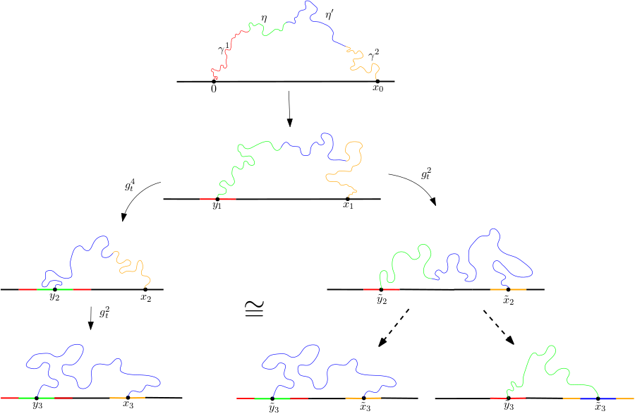
We write ϵ=s−r\epsilon=s-r. We decompose a simple path γ\gamma from 00 to xx with hcap⁡[γ]=a{\rm hcap}[\gamma]=a as

γ=γ1⊕η⊕(η′)R⊕(γ2)R,\gamma=\gamma^{1}\oplus\eta\oplus(\eta^{\prime})^{R}\oplus(\gamma^{2})^{R},

where the decomposition is defined by

hcap⁡[γ1]=r​a,hcap⁡[γ1∪η]=s​a,hcap⁡[γ1∪γ2]=(t0−ϵ)​a.{\rm hcap}[\gamma^{1}]=ra,\;\;\;\;\;{\rm hcap}[\gamma^{1}\cup\eta]=sa,\;\;\;\;\;\;\;\;{\rm hcap}[\gamma^{1}\cup\gamma^{2}]=(t_{0}-\epsilon)a.

Using the definition and the conformal Markov property, we can see that when we sampling from μs\mu_{s} we choose the paths in order γ1,η,γ2,η′\gamma^{1},\eta,\gamma^{2},\eta^{\prime}. When we sample from μr\mu_{r} we use the order γ1,γ2,η′,ηR\gamma^{1},\gamma^{2},\eta^{\prime},\eta^{R}. In each case the distribution is S​L​ESLE to the endpoint of the other curve in the domain slit by the curves at that point, conditioned to have the appropriate total half-plane capacity and stopped as specified above.

We now use Proposition 3.1 to say that another way to sample from μs\mu_{s} is to choose the paths in order γ1,γ2,η,η′\gamma^{1},\gamma^{2},\eta,\eta^{\prime}. Hence we can write the sampling as follows. Steps 1 and 2 are the same for both sampling methods. Step 3a is used for μs\mu_{s} and Step 3b is used for μr\mu_{r}.

  • •

    Step 1: Choose γ1\gamma^{1} from S​L​ESLE from 00 to x0x_{0} conditioned to have total half-plane capacity aa stopped at time rr, that is, stopped when hcap⁡[γ1]=a​r{\rm hcap}[\gamma^{1}]=ar. Let z1=γ⁡(r)z_{1}=\gamma(r), let g^:ℍ∖γ1→ℍ\hat{g}:{\mathbb{H}}\setminus\gamma^{1}\rightarrow{\mathbb{H}} be the corresponding transformation, and let y1=g^​(z1),x1=g^​(x0)y_{1}=\hat{g}(z_{1}),x_{1}=\hat{g}(x_{0}).

  • •

    Step 2: Choose η\eta from S​L​ESLE from x1x_{1} to y1y_{1} conditioned to have total half-plane capacity a⁡(1−r)a(1-r) stopped at time 1−s1-s, that is, stopped when hcap⁡[η]=a⁡(1−s){\rm hcap}[\eta]=a(1-s). Let h:ℍ∖η→ℍh:{\mathbb{H}}\setminus\eta\rightarrow{\mathbb{H}} be the corresponding transformation, and let y2=h⁡(y1),x2=h⁡(η⁡(1−s))y_{2}=h(y_{1}),x_{2}=h(\eta(1-s)). Let γ2=g^−1∘η\gamma^{2}=\hat{g}^{-1}\circ\eta and w1=g−1​(η⁡(1−s))w_{1}=g^{-1}(\eta(1-s)). Let h^=h∘g\hat{h}=h\circ g and note that h^:ℍ∖(γ1∪γ2)→ℍ\hat{h}:{\mathbb{H}}\setminus(\gamma^{1}\cup\gamma^{2})\rightarrow{\mathbb{H}} is the corresponding conformal transformation which satisfies h^​(z1)=y2,h^​(w1)=x2\hat{h}(z_{1})=y_{2},\hat{h}(w_{1})=x_{2}.

  • •

    Step 3a: Choose ω1\omega^{1} from S​L​ESLE from y2y_{2} to x2x_{2} conditioned to have total half-plane capacity a​ϵa\epsilon stopped at the first time that

    hcap⁡[h−1∘ω1]=a​ϵ.{\rm hcap}[h^{-1}\circ\omega^{1}]=a\epsilon.

    This is the same as the first time that

    hcap⁡[γ1∪h^−1∘ω1]=a​s.{\rm hcap}[\gamma^{1}\cup\hat{h}^{-1}\circ\omega^{1}]=as.

    Let this time be uu and let ϕ:ℍ∖ω1→ℍ\phi:{\mathbb{H}}\setminus\omega^{1}\rightarrow{\mathbb{H}} be the corresponding transformation with y3=ϕ⁡(ωu1),x3=ϕ⁡(x2)y_{3}=\phi(\omega^{1}_{u}),x_{3}=\phi(x_{2}). Let ω~2\tilde{\omega}^{2} be chosen from S​L​ESLE from x3x_{3} to y3y_{3} conditioned to have half-plane capacity a⁡(ϵ−u)a(\epsilon-u) giving conformal map ϕ^\hat{\phi} and let ω2=ϕ^−1∘ω~2\omega^{2}=\hat{\phi}^{-1}\circ\tilde{\omega}^{2} and

    ω=ω1⊕[ω2]R.\omega=\omega^{1}\oplus[\omega^{2}]^{R}.

    Let ψ:ℍ∖ω→ℍ\psi:{\mathbb{H}}\setminus\omega\rightarrow{\mathbb{H}} be the corresponding conformal transformation.
    Refer to caption
    Figure 4: A schematic showing the full picture, though not drawn to scale (in particular, the yellow and blue segments ought not to have comparable lengths). The dotted arrows on the right correspond to the commutation relation, and together with some Loewner estimates, we may conclude that the laws of the measures obtained, regardless of the path one chooses in the schematic, are the same.
  • •

    Step 3b Choose ω∗\omega^{*} from S​L​ESLE from x2x_{2} to y2y_{2} conditioned to have total half-plane capacity a​ϵa\epsilon and set

    ω^=[ω∗]R.\hat{\omega}=[\omega^{*}]^{R}.

    Let ψ^:ℍ∖ω^→ℍ\hat{\psi}:{\mathbb{H}}\setminus\hat{\omega}\rightarrow{\mathbb{H}} be the corresponding conformal transformation.

In our coupling we use the complete coupling for steps 1 and 2. Hence we write

g=ψ∘h,g~=ψ~∘h,g=\psi\circ h,\;\;\;\;\;\tilde{g}=\tilde{\psi}\circ h,

where hh is the same in both cases. If z∈ℐz\in{\mathcal{I}}, then Im⁡(h⁡(z))≥4​a{\rm Im}(h(z))\geq\sqrt{4a}. Except for an event of probability that decays faster than every power of ϵ\epsilon, we have x2−y2≤ϵ1/2​log⁡(1/ϵ)x_{2}-y_{2}\leq\epsilon^{1/2}\,\log(1/\epsilon). Using this, we see that in step 3a and in step 3b we get a curve with the same initial and terminal points, of half plane capacity a​ϵa\epsilon and such that, except for an event of probability that decays faster than every power of ϵ\epsilon, has diameter bounded by ϵ1/2​log2​ϵ\epsilon^{1/2}\,\log^{2}\epsilon. Let ψ,ψ~\psi,\tilde{\psi} be the conformal transformations. Then if Im⁡(z)≥a{\rm Im}(z)\geq\sqrt{a} we have

|ψ⁡(z)−ψ~​(z)|≤c​ϵ,|\psi(z)-\tilde{\psi}(z)|\leq c\,\epsilon,

and, except for an event of probability that decays faster than every power of ϵ\epsilon,

|ψ⁡(z)−ψ~​(z)|≤ϵ5/4.|\psi(z)-\tilde{\psi}(z)|\leq\epsilon^{5/4}.

Therefore, in this coupling, with probability one ‖g−g~‖≤c​ϵ\|g-\tilde{g}\|\leq c\,\epsilon and

ℙ{∥g−g~∥≥ϵ5/4}≤cϵ3.{\mathbb{P}}\{\|g-\tilde{g}\|\geq\epsilon^{5/4}\}\leq c\,\epsilon^{3}.

5 Proof of Lemma 2.2

We fix a>1/4a>1/4 and allow constants to depend on aa. We assume that XtX_{t} satisfies (7). For ease we will assume x>0x>0 but the proof with x<0x<0 is essentially the same.

The proof follows from the easy estimate

−Xt≤Ut≤∫0taXs​𝑑s-X_{t}\leq U_{t}\leq\int_{0}^{t}\frac{a}{X_{s}}\,ds

and the following two lemmas that handle the two sides of the inequality. For the lower bound, we get a somewhat sharper estimate.

Lemma 5.1.

There exists c<∞c<\infty such that if XtX_{t} satisfies (7) with X0=x0​t0>0,X_{0}=x_{0}\,\sqrt{t_{0}}>0, then for all r>0r>0,

ℙ{max0≤t≤t0(Xt/t0)≥x0+r}≤cexp{−r24}.{\mathbb{P}}\left\{\max_{0\leq t\leq t_{0}}(X_{t}/\sqrt{t_{0}})\geq x_{0}+r\right\}\leq c\,\exp\left\{-\frac{r^{2}}{4}\right\}.
Proof.

We may assume that r2≥1+4​ar^{2}\geq 1+4a and by scaling we may assume t0=1t_{0}=1. Let y=x0+ry=x_{0}+r and let σ=inf{t:Xt=y}.\sigma=\inf\{t:X_{t}=y\}. The equation (7) can be obtained by starting with XtX_{t} satisfying (3) where WtW_{t} is a ℙ∗{\mathbb{P}}^{*} Brownian motion and then tilting by the martingale NtN_{t} as in (6) to get the measure ℙ{\mathbb{P}}. Hence,

ℙ{σ<1}≤M0−1𝔼∗[Mσϵ;σϵ<∞].{\mathbb{P}}\{\sigma<1\}\leq M_{0}^{-1}\,{\mathbb{E}}^{*}\left[M_{\sigma_{\epsilon}};\sigma_{\epsilon}<\infty\right].

Note that

M0=x04​a−1​exp⁡{−x022},M_{0}=x_{0}^{4a-1}\,\exp\left\{-\frac{x_{0}^{2}}{2}\right\},

and if σ<1\sigma<1,

Mσ≤max0≤t≤1y4​a−1(1−t)−12−2​aexp{−y22​(1−t)}=y4​a−1e−y2/2.M_{\sigma}\leq\max_{0\leq t\leq 1}y^{4a-1}\,(1-t)^{-\frac{1}{2}-2a}\,\exp\left\{-\frac{y^{2}}{2(1-t)}\right\}=y^{4a-1}\,e^{-y^{2}/2}.

The equality uses r2≥1+4​ar^{2}\geq 1+4a. Therefore,

MσM0≤[1+log⁡(1/ϵ)x0]4​a−1​exp⁡{−x0​r−r22}≤c​exp⁡{−r24}.\frac{M_{\sigma}}{M_{0}}\leq\left[1+\frac{\log(1/\epsilon)}{x_{0}}\right]^{4a-1}\,\exp\left\{-x_{0}\,r-\frac{r^{2}}{2}\right\}\leq c\,\exp\left\{-\frac{r^{2}}{4}\right\}.

∎

Lemma 5.2.

If a>1/4a>1/4, there exist u>0u>0 and c<∞c<\infty such that for any x>0x>0 and t0>0t_{0}>0 if XtX_{t} satisfies (7), then for all r>0r>0,

ℙx{∫0t0d​sXsdy≥rt0}≤ce−u​r.{\mathbb{P}}^{x}\left\{\int_{0}^{t_{0}}\frac{ds}{X_{s}}\,dy\geq r\sqrt{t_{0}}\right\}\leq c\,e^{-ur}.
Proof.

Let

In=∫01d​sXs 1{2−n≤Xs<2−n+1}ds.I_{n}=\int_{0}^{1}\frac{ds}{X_{s}}\,1\{2^{-n}\leq X_{s}<2^{-n+1}\}\,ds.

Our first goal is to show that there exists c∗<∞c_{*}<\infty such that for all x,t0,nx,t_{0},n,

𝔼x[In]≤c∗ 2−n,ℙx{In≥c∗ 2−n+1}≤12.{\mathbb{E}}^{x}[I_{n}]\leq c_{*}\,2^{-n},\;\;\;\;\;{\mathbb{P}}^{x}\{I_{n}\geq c_{*}\,2^{-n+1}\}\leq\frac{1}{2}. (9)

The second follows from the first by the Markov property; by scaling, It suffices to show the first inequality for n=0n=0. By the strong Markov property. we may assume that 1≤x≤21\leq x\leq 2; otherwise, we first run the process until it reaches [1,2][1,2]. Also, note that

𝔼x​[I0]≤∫12∫0t0ϕt​(x,y,t0)​𝑑t​𝑑y.{\mathbb{E}}^{x}[I_{0}]\leq\int_{1}^{2}\int_{0}^{t_{0}}\,\phi_{t}(x,y;t_{0})\,dt\,dy.

Using the immediate estimate

∫12[∫t0−1t0ϕt​(x,y,t0)​𝑑t+∫01ϕt​(x,y,t0)​𝑑t]​𝑑y≤2,\int_{1}^{2}\left[\int_{t_{0}-1}^{t_{0}}\,\phi_{t}(x,y;t_{0})\,dt+\int_{0}^{1}\,\phi_{t}(x,y;t_{0})\,dt\right]dy\leq 2,

we see that it suffices to show that there exists cc such that for all 1≤x,y≤21\leq x,y\leq 2 and t0≥1t_{0}\geq 1,

∫1t0−1ϕt​(x,y,t0)​𝑑t≤c.\int_{1}^{t_{0}-1}\phi_{t}(x,y;t_{0})\,dt\leq c.

This can be done in a straightforward way by looking at the transition probability. Indeed, if 1≤s≤t0−11\leq s\leq t_{0}-1 and 1≤x,y≤21\leq x,y\leq 2,

ϕt​(x,y,t0)≤c​[t0t0−t]2​a+12​1t2​a+12.\phi_{t}(x,y;t_{0})\leq c\,\left[\frac{t_{0}}{t_{0}-t}\right]^{2a+\frac{1}{2}}\,\frac{1}{t^{2a+\frac{1}{2}}}.

For t<t0/2t<t_{0}/2 we estimate this by c​t−(2​a+12)c\,t^{-(2a+\frac{1}{2})} and for t≥t0/2t\geq t_{0}/2, we estimate this by c​(t0−t)−(2​a+12).c\,(t_{0}-t)^{-(2a+\frac{1}{2})}. Provided that a>1/4a>1/4 we see that this integral is uniformly bounded in t0t_{0}. This gives (9).

By scaling it suffices to prove our main result for t0=1t_{0}=1. Note that

∫01d​sXs​𝑑s≤1+∑n=1∞In,\int_{0}^{1}\frac{ds}{X_{s}}\,ds\leq 1+\sum_{n=1}^{\infty}I_{n},

where

In=∫01d​sXs 1{2−n≤Xs<2−n+1}ds.I_{n}=\int_{0}^{1}\frac{ds}{X_{s}}\,1\{2^{-n}\leq X_{s}<2^{-n+1}\}\,ds.

By iterating (9) using the strong Markov property, we see that for all positive integers kk, ℙ{In≥2kc∗ 2−n}≤2−k{\mathbb{P}}\{I_{n}\geq 2k\,c_{*}\,2^{-n}\}\leq 2^{-k} and hence for all r>0r>0,

ℙ{In≥r 2−n}≤c′e−u​r,{\mathbb{P}}\{I_{n}\geq r\,2^{-n}\}\leq c^{\prime}\,e^{-ur},

where u=(log⁡2)/(2​c∗),c′=euu=(\log 2)/(2c_{*}),c^{\prime}=e^{u}. In particular,

ℙ{∑n=1∞In≥2r}≤∑n=1∞ℙ{In≥r(2/3)n}≤c′∑n=1∞exp{−ur(4/3)n}≤ce−2u(2r)/3.{\mathbb{P}}\left\{\sum_{n=1}^{\infty}I_{n}\geq 2r\right\}\leq\sum_{n=1}^{\infty}{\mathbb{P}}\left\{I_{n}\geq r(2/3)^{n}\right\}\leq c^{\prime}\sum_{n=1}^{\infty}\exp\left\{-ur(4/3)^{n}\right\}\leq c\,e^{-2u(2r)/3}.

∎

References

  • [1] Julien Dubédat. Duality of Schramm-Loewner evolutions. Ann. Sci. Éc. Norm. Supér. (4), 42(5):697–724, 2009.
  • [2] Gregory F. Lawler. Conformally invariant processes in the plane, volume 114 of Mathematical Surveys and Monographs. American Mathematical Society, Providence, RI, 2005.
  • [3] Jason Miller and Scott Sheffield. Imaginary geometry I: interacting SLEs. Probab. Theory Related Fields, 164(3-4):553–705, 2016.
  • [4] Jason Miller and Scott Sheffield. Imaginary geometry II: Reversibility of SLEκ⁡(ρ1;ρ2)\operatorname{SLE}_{\kappa}(\rho_{1};\rho_{2}) for κ∈(0,4)\kappa\in(0,4). Ann. Probab., 44(3):1647–1722, 2016.
  • [5] Jason Miller and Scott Sheffield. Imaginary geometry III: reversibility of SLEκ\mathrm{SLE}_{\kappa} for κ∈(4,8)\kappa\in(4,8). Ann. of Math. (2), 184(2):455–486, 2016.
  • [6] Dapeng Zhan. Reversibility of chordal SLE. Ann. Probab., 36(4):1472–1494, 2008.