Path Verification for Dynamic Indirect IlluminationJournal: TOGCCS: Computing methodologies Ray tracingCCS: Computing methodologies Rendering

Pierre Moreau Affiliation: Lund University, Sweden , Michael Doggett Affiliation: Lund University, Sweden and Erik Sintorn Affiliation: Chalmers University of Technology, Sweden

Refer to caption — Figure 1. Rendering in the Villa scene for the baseline on the left, and our error-based method on the right at roughly equal frame time (341 ms, and resp. 333 ms); in both cases, the number of bounces is limited to 7. The baseline traces 3 million paths in about 178 ms, and the splatting of the photons takes 148 ms. On the other hand, our method traces and reuses 5 million paths in about 80 ms, and the splatting of the photon takes 236 ms.

Abstract.

In this paper we present a technique that improves rendering performance for real-time scenes with ray traced lighting in the presence of dynamic lights and objects. In particular we verify photon paths from the previous frame against dynamic objects in the current frame, and show how most photon paths are still valid. When using area lights, we use a data structure to store light distribution that tracks light paths allowing photons to be reused when the light source is moving in the scene. We also show that by reusing paths when the error in the reflected energy is below a threshold value, even more paths can be reused. We apply this technique to Indirect Illumination using a screen space photon splatting rendering engine. By reusing photon paths and applying our error threshold, our method can reduce the number of rays traced by up to 5 $\times$ , and improve performance by up to 2 $\times$ .

Keywords:

Photon Mapping, Global Illumination

\footnotetextcopyrightpermission

1. Introduction

Indirect illumination is an important cue for the perceived realism of computer generated imagery, but its accurate computation can be computationally expensive. A recent survey by Ritschel et al. (Ritschel et al. 2012) covers many algorithms that approximate indirect illumination for real-time applications. Since the general problem is complex, and cannot be easily solved even in offline rendering, where hundreds of cores can spend hours on a single frame, most real-time algorithms are specifically designed to generate a good estimation under very specific assumptions about lighting and materials.

Computing indirect illumination and soft shadows, while considering animated objects, leads to a more accurate representation of the lighting in a scene, than can usually be achieved with pre-computed techniques. In this paper we build upon the photon splatting technique by Moreau et al. (Moreau et al. 2016) to enable indirect lighting with multiple dynamic light sources. Unlike Moreau et al. (Moreau et al. 2016), where the photon map is recomputed every frame, we propose to opportunistically reuse as many photon paths as possible, including those from moving light sources. We achieve this by reusing lighting from previous frames, and within area lights. In this paper we present a technique that uses a photon map with several bounces, many more than previous techniques, enabling subtle lighting effects in neighboring areas which have no direct path to the light source.

Photon mapping traces light paths from the light, and deposits photon energy onto diffuse surfaces. To create the final image, camera rays are traced to gather the light deposited on surfaces in the scene. Path tracing instead traces rays from the camera through the scene until they find a light source. This means that for traditional path tracing, all segments of a path must be verified if lights or objects move in the scene. While for photon mapping, only the light paths from the light to the surface need to be verified, as camera rays will be traced regardless.

In scenes with moving objects and dynamic light sources, we present techniques for path verification. If a path from a previous frame is classified as still valid, we reuse the photon path in the current frame. By reusing photon paths we are able to achieve interactive frame rates in scenes with indirect illumination. Unlike previous methods with geometric approximations or sparse samples sets, we use a dense photon map, and instead of recomputing all light per frame, including lighting that is still valid, we carefully reuse the light transport from the previous frame.

Using photon maps allows indirect illumination to be computed in world space without the limitations of screen space methods, and enables the possibility to temporally reuse light transport computations from previous frames.

2. Related Work

Early attempts to achieve precomputed light transport stored it in textures (McTaggart 2004), or used spherical harmonics to store precomputed light transport (Sloan et al. 2002), or, more recently, in precomputed light field probes (McGuire et al. 2017). These algorithms can be very efficient to query, but require significant computational resources for offline precomputations, and large memory buffers for high quality results. More importantly, they do not allow for dynamic lights. On the other end of the spectra are screen space reflection algorithms (Sousa et al. 2011) that can very quickly estimate the radiance reflected from a glossy material, but only when the reflected surfaces are directly visible to the user. Other screen space algorithms (Ritschel et al. 2009) are only effective for local reflections when the material is lambertian and do not take into account more complex materials or light sources outside of the viewing volume.

Dmitriev et al. (Dmitriev et al. 2002) used two different types of photons to detect areas where lighting changed between frames, and focused updates to the lighting in those regions using corrective photons. This allows them to support dynamic scenes and prioritise the updates to perform, however each corrective photons needs to be traced twice, with one of the tracings taking place against an earlier version of the scene.

To reduce the number of paths needed per pixel, Bekaert et al. (Bekaert et al. 2002) proposed creating path segments in neighboring pixels and sharing those paths to increase the number of paths traced in each individual pixel. While our work also attempts to reduce computation per frame by reusing paths, we reuse the photon paths from the previous frame, not neighboring pixels.

Voxel Cone Tracing (Crassin et al. 2011) alleviates both of these problems by voxelizing a rough representation of the scene around the user’s position, and can be used for diffuse indirect illumination, but is much too expensive in terms of memory to allow for large scenes. Also this algorithm does not allow for many bounces of light.

Also dynamic scenes have been mixed with Stochastic Progressive Photon Mapping (Weiss and Grosch 2012), but this is a much more complex technique and requires much longer frame times than our technique.

More recently, several denoising algorithms have been suggested, that allow for fast denoising of extremely noisy path-traced images (Chaitanya et al. 2017; Schied et al. 2017; Mara et al. 2017). By filtering samples both spatially and temporally, the reflected radiance of each pixel can be estimated almost as well as if hundreds of indirect illumination rays had been shot per pixel and can handle both glossy and diffuse surfaces. While these approaches can generate path traced images at real-time rates, they use short path lengths to ensure performance.

Another recent method is that of Silvennoinen et al. (Silvennoinen and Lehtinen 2017) where a very sparse set of light probes are updated every frame by shooting a single ray per direction and looking up the intersected surface’s direct-lighting response in a texture. Our technique robustly checks all dynamic objects, unlike Silvennoinen et al. (Silvennoinen and Lehtinen 2017), which only has support for approximated dynamic objects and so will fail to correctly capture the illumination when all light has undergone several bounces before reaching the camera.

Corso et al. (Corso et al. 2017) recently looked into reusing shading information at primary view samples from previous frames. This is done by reprojecting the view sample locations into the current frame and validating their visibility. They also maintain a uniform distribution of outgoing rays to avoid having too many or too few paths at a given pixel. Our approach extends the validation to consider the whole path rather than just the first segment, and we modified how the uniform distribution is maintained to apply to light sources and support area lights.

3. Algorithm

Figure 2. A simple scene showing an area light source at the top, show as a grid, from which several photon paths are traced. A small cube moves in the bottom of the scene, shown in it’s starting position on the left, and it’s new position on the right. In the right image the cube intersects the existing segments of all paths. The grid at the top represents what we call a distribution map covering the two dimensional area light. For the green and blue paths, as only their last segment is being intersected, we only need to compute the new intersection point. On the other hand, the red path’s first segment is intersected also triggering a computation of the new intersection point, but also a resampling of the BRDF there, due to the second photon having become invisible from the first one. However, since the new second photon can see the old third one, and the energy between the two is similar to before, the third photon is kept as-is.

Figure 3. A diagram showing where our algorithm sits in a regular photon renderer, visualised as a grey box, as well as its different main steps. The green box groups steps involving distribution maps together, whereas the blue box groups all steps needed for reusing photons from frame to frame. The “generate rays” and “trace rays” steps bare a few differences in our algorithm, compared to the classic version. However, as those are not significant, they are represented as the same steps in this diagram; the differences will be presented in Section 4.

DM_{C}

represents the distribution map of the current frame, computed from the existing light paths.

Given a scene made only of static objects and lights, the tracing of the light paths only needs to be done once and can be reused for all frames. In this paper we focus on the reuse of light paths from previous frames in the presence of dynamic objects and lights, and are not concerned with static scenes. To verify that a light path is still valid in the current frame, it must be checked against moving objects and light sources. Figure 2 illustrates how the algorithm handles a single moving object intersecting three photon paths. In this section we outline how this verification of light paths is performed first for dynamic lights, and then for dynamic objects.

Our algorithm is made of 5 main steps, that process all light paths from previous frames and tell a slightly modified photon mapper/splatter which paths should be retraced; details about the modifications done to the photon mapper/splatter can be found in Section 4. In the following we give a brief introduction to the five main stages of our algorithm, and then explain them in more detail later in this section.

Update path origins:: to match the current position and orientation of light sources.
Dynamic occlusions:: will detect and schedule for re-tracing paths intersected by dynamic objects.
Compute $DM_{C}$ :: to know how many light paths are emitted from each cell.
Prune paths:: to decrease the number of emitted paths for cells with too many light paths.
Fill $DM_{C}$ :: to increase the number of light paths in cells below the required amount.

Apart from “dynamic occlusions”, which will be presented in Section 3.2 as it is unnecessary for dynamic lights, the remaining four main steps will be presented in Section 3.1. Figure 3 shows the structure of the five steps and where they sit in relation to a regular photon splatting architecture.

3.1. Supporting dynamic lights

As lights move in a scene, some surfaces that were previously unlit become now visible to a light source and receive light, while others fade in the shadows. To validate light paths against such behaviours, a first approach would be to test whether the primary segment of each path is still within the light’s field of view, and if not, replace the whole path by a new one. However this can lead to changes in the light’s distribution, as showcased in Figure 4.

Even a light that moves parallel to the plane it is illuminating, will have issues if photons that are now no longer visible from the light are randomly re-traced over the whole volume visible from the light. This would result in very few photons in the newly visible areas, as many of the new photons would end up in the already visible areas. To avoid those issues, we propose to maintain the distribution of photons from the light source between frames.

To achieve equal distribution across the light we partition its surface, and its set of outgoing directions into cells, and ensure that each cell maintains a given amount of primary paths emitted from that cell. Those cells form an $n$ -D array which we call a Distribution Map (DM). The parametrisation of this array is not constrained and can be different for different light types. For example, a point light could have a 2-D parametrisation $(\theta,\phi)$ whereas a rectangular area light could use a 4-D parametrisation $(x,y,\theta,\phi)$ ; an example of parametrisation for a 2-D spotlight can be seen in Figure 5.

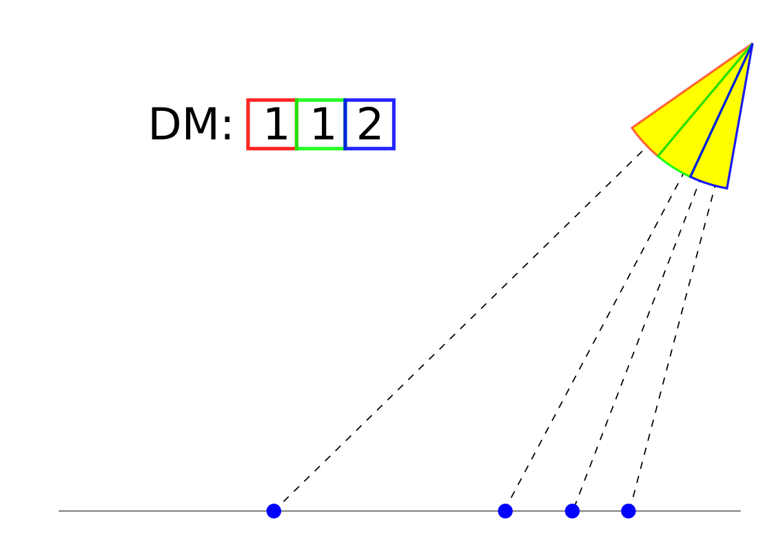
The distribution map is initialised with a user-defined distribution for the light source. This initial set of values is denoted as $DM_{T}$ , or the targeted distribution of the light. This target distribution could be updated every frame to allow for textured light sources. A second distribution map, noted $DM_{C}$ , is computed each frame using all existing paths at the end of the previous frame. Each frame, we apply a set of operations to make $DM_{C}$ converge towards $DM_{T}$ ; those operations might update the values stored in $DM_{C}$ to ensure that it counts only valid paths.

Update path origins

As the lights move, we need to update the position on the light from which the paths are emitted. For a point light, this simply means setting the light sample to the new position of the light and recomputing the outgoing direction based on this new position and the existing primary photon. We also check that the primary photon is still visible from the light, by making use of the attached shadow map. This will however not work for area lights, so in those cases, to avoid tracing visibility rays towards each primary photon, we keep the existing outgoing direction and compute its intersection with the plane of the light to get the new origin of the path. Some of the light paths can already be invalidated during this step.

Compute $DM_{C}$

As the light path origins have been updated to reflect the current position and orientation of the lights, we can now compute how many light paths are emitted from each cell; this is done for all paths that were successfully updated in the previous step. If the parametrisation function of the distribution map returns a correct value given the position on the light and outgoing direction of a light path, the cell found to have emitted this path is atomically increased. Otherwise, the path is marked as invalid and will be re-traced in the “fill $DM_{C}$ ” step.

Prune paths

Thanks to the previous step, we now know how many paths lie in each cell. Some of them might contain more paths than they should, if the light moved. In order to converge back to $DM_{T}$ , for each cell where $DM_{C}>DM_{T}$ , every path emitted from that cell will be pruned with the following probability:

(1)

\frac{DM_{C}-DM_{T}}{DM_{C}}

note that this does not ensure that $DM_{C}$ will be equal to $DM_{T}$ , but ensures that $DM_{C}$ will converge towards the target over a number of frames. Also, all paths pruned by this pass are valid paths: we could keep them and reduce their energies, however that could result over time in paths with low energy, so we prune them instead.

Fill $DM_{C}$

For the same reasons that some cells will contain more paths, others will be lacking some paths. For each cell to reach its expected amount of paths, we sample the light to obtain a new position on the light and outgoing direction. The sampling of the light is restricted to the domain contained within the cell. Those inputs will later be used to trace new light paths in the “trace rays” step.

3.2. Supporting dynamic objects

To handle dynamic objects, the “dynamic occlusions” step of the algorithm adds visibility rays to compute whether the visibility between two vertices of the path changed. These rays test the current segment against the bounding box of every dynamic object in the scene, and kill the segment if any of the tests fail. This is a conservative approach and might return false positives.

In order to avoid unnecessary tests, we test the segments of a path in order, starting from the segment leaving the light. If the $i$ th segment of the path is intersected by a dynamic object, all segments after it will be different. After a segment is found to be intersected by a dynamic object, we schedule that segment and all the following ones to be re-traced.

3.3. Error-based threshold for path reuse

While the solution presented in Section 3.2 is straightforward, some paths propagate very similar energy from frame to frame and could be reused. Instead of killing the intersected segment $i$ , we trace a visibility ray from the segment’s origin to it’s destination, and compute the new end of that segment, which is also the origin of the next segment $j$ . As we updated the origin of $j$ , we may break the visibility between both ends of that segment. We can trace a new visibility ray along $j$ to compute its new end point, and continue similarly until we reach the end of the path. The error-based threshold algorithm is shown in Algorithm 1.

We can however avoid the visibility ray under certain circumstances: if the segment is not intersected by any dynamic objects, neither its origin nor end are located on dynamic objects, and its newly computed origin is located at the same position as its old origin. This situation can occur when segment $i$ is intersected by the bounding box of a dynamic object, but in practice is not intersected by any of the object’s triangles.

When reusing path vertices, sometimes the energy reflected $E_{N}$ , at the new intersection point is very similar to how much energy $E_{O}$ , was being reflected at the old intersection point. We detect these cases by using a user specified energy threshold $T$ , and if Equation 2 is satisfied, we don’t update or propagate the new energy value saving valuable computation time. Otherwise, all the segments — starting from the current vertex — are re-traced. By always comparing $E_{N}$ to the original reflected energy $E_{O}$ , we ensure that we do not accumulate errors for the energy over multiple frames.

(2)

(-T\times E_{O}\leq E_{N}-E_{O})\land(E_{N}-E_{O}\leq T\times E_{O})

This technique will never trace more rays than if the whole path had been invalidated, and can improve the temporal coherency by reusing some of the segments.

// For each path, iterate over its segments, starting from the first one.

foreach $Segment\in Path$ do 1

if $\textnormal{{not}}IntersectedByObjects(Segment)$ then 2

continue // Compute intersection along segment

Hit\leftarrow TraceRay(Segment.origin,Segment.dir)

HitPos\leftarrow ComputeHitPos(Segment,Hit)

NextSeg\leftarrow Next(Segment,Path)

// Compute new outgoing direction

NextSeg.origin\leftarrow HitPos

NextSeg.dir\leftarrow NextSeg.dest-NextSeg.origin

Energy\leftarrow BRDF(Segment,NextSeg)

if $\textnormal{{not}}AreEnergiesClose(NextSeg.energy,Energy)$ then 9

Segment.dest\leftarrow HitPos

// Sample BRDF to generate new ray

return else if $AreClose(HitPos,Segment.dest)\land\textnormal{{not}}IntersectedByObjects(NextSeg)\land\textnormal{{not}}HitMovingObject(NextSeg.origin)\land\textnormal{{not}}HitMovingObject(NextSeg.dest)$ then 11

// Skip visibility check between NextSeg.origin and NextSeg.dest

Segment\leftarrow NextSeg

continue

Segment.dest\leftarrow HitPos

// Visibility check for NextSeg will occur on the next iteration

Algorithm 1 Error-based threshold approach to dynamic occlusions handling

4. Implementation details

Each path is made up of several photons, and in order to keep track of the paths’ structure, including the photon order, we store the photons in a 2-D array where the $i$ -th row contains the $i$ -th photon of a path, and each column is a different path. This memory layout, rather than its transpose, allows for better memory access patterns, as all threads loading their $i$ -th photon will result in consecutive memory accesses. Photons use a total of 32 bytes:

•

Incoming direction (as XYZ): 3 floats;
•

ID of object hit: 32-bit integer;
•

Energy (as RGB): 3 floats;
•

Radius: float.

To help with the current status of a path, we store separately a small data structure (a single 32-bit word) containing the following:

•

The ID of the $DM_{C}$ ’s cell in which this path lies. (22 bits);
•

The number of segments in the path. (4 bits);
•

Starting segment to retrace path from. (4 bits);
•

Replace path. The path is retraced if the bit is set. (1 bit);
•

Reuse light keeping light position and direction. (1 bit).

The representation of the different steps as seen in Figure 3 does not match 1:1 to our implementation. For example, we actually update the path origins and compute the $DM_{C}$ in the same kernel, while the dynamic occlusions are tested right after that. The merging of the two kernels was done for performance reasons, in order to avoid reading from memory data that was recently written, and the two kernels were relatively small. Since the dynamic occlusions testing can not be done before the path origins are updated, it had to be moved after the computation of the $DM_{C}$ .

For simplicity reasons, we generate new rays as soon as it has been decided we need to replace an existing ray. This means that ray generation is effectively done in multiple places: during the dynamic occlusions testing, when filling the $DM_{C}$ and when processing the results from the tracing pass, if the maximum depth has not been reached yet.

Finally, when pruning extra paths, we end up modifying the number of paths found in the distribution map, while needing to use the initial amount in the pruning probability (see Equation (1)). This can be achieved by modifying a copy of the distribution, thus using more memory, or by doing the update in two passes by first marking the pruned paths, and then editing the distribution map values. We are using the second approach in our implementation.

5. Results

All presented results were rendered at a resolution of $1920\times 1080$ on an NVIDIA Titan X (Pascal architecture, 12 GB of VRAM). The tracing of the photons was done using OptiX Prime 5.0.0 (Parker et al. 2010), whereas the path-reuse computations were implemented using CUDA 9.1 (Nickolls et al. 2008). We compare our “naive” approach, presented in Section 3.2, to our error-based method, presented in Section 3.3 and to a baseline, which consists in not reusing any information from previous frames and re-tracing every single path each frame.

We tested our methods on different scenes:

Merry-go-round:: Conference, with a disc area light placed above the centre of the conference table, 3 scaling and rotating teapots placed on that table, around which 8 bunnies move as shown in Figure 6a);
Armadillo:: Conference scene with an armadillo moving from one door to the presenter stand, waiting there for a few seconds, then proceeding to the other door as shown in Figure 6b.
Villa:: a small torchlight, made of a disc-shaped area light, is moving within the kitchen of a house, indirectly lighting the living room as shown in Figure 6c.

We recorded the first 30 seconds of the rendering of each scene, for the baseline and our two methods; those videos can be found in the supplemental materials. The configurations used (number of paths, resolution of the DM, etc.) are the same as the ones mentioned in Figure 7. Note that the time displayed in the top-right corner in the videos corresponds to the total frame time, while Figure 7 and 8 both focus on only a few steps of the process, ignoring for example the time taken for splatting the photons ( $\geq 130$ ms) as orthogonal to the reuse.

5.1. Performance

The breakdowns presented in Figure 8 uses the different categories presented in Figure 3, but with the modifications described in Section 4. So, for example, the “update path origins” time is included within the “compute $DM_{C}$ ” time, as they are implemented within the same kernel.

Our two methods only differ in how they handle moving objects, but their handling of moving lights is the same. This explains why there is no differences between our two methods, neither in number of rays reused nor in tracing time, in Figure 7c.

Even our naive method for dynamic objects already significantly reduces the number of rays traced each frame, for example for the armadillo scene, it is reduced by 5 $\times$ , as can be seen in Figure 7b. This does not translate into a 5 $\times$ decrease in the time taken by OptiX prime for tracing those rays, but into a 3 $\times$ decrease instead. This could come from more primary rays, proportionally, not being retraced, compared to secondary rays, which are more expensive, as well as not taking special care to maximise ray locality and coherency. Overall, our error-based method only slightly improves the number of rays reused, except when the armadillo gets close to the light source (around frame 250), where it retraces only half the number of rays compared to our naive method.

The merry-go-round scene reduces the effectiveness of ray reuse, as many primary rays will be hitting a moving object, instantly invalidating the whole path. Despite that, our naive method queries almost half as many rays as the baseline. Furthermore, our error-based approach reuses close to 1.5 $\times$ as many rays as our naive approach, as seen in Figure 7a.

Our different methods do add a small overhead compared to just re-tracing the paths every frame. This overhead includes updating the path’s origin, computing the $DM_{C}$ and optimising it. On average the overhead is about 2.5 ms, compared to the average baseline time of 60 ms, as shown in Figure 8, and even including this overhead our method still leads to an average 4 $\times$ increase in performance.

(a) Merry-go-round

(b) Armadillo

Figure 7. Tracing time and number of rays compared to the baseline, for the different scenes. The merry-go-round and armadillo scenes both used 2 million paths, whereas the villa has 1 million paths, but for all of them the paths contained at most 7 photons and the distribution map had a resolution of

8\times 8\times 64\times 64

. For our error-based method, the energy threshold was set to 0.1%.

(a) Our error-based method

(b) Baseline

Figure 8. Breakdowns of our method for reusing photons (top) and of the baseline (bottom), for the armadillo scene. In both cases, 2 m paths were traced with a maximum of 7 bounces, and for our method, the distribution map had a resolution of

8\times 8\times 64\times 64

while a 0.1% error on the outgoing radiance was allowed on reused segments.

5.2. Memory Consumption

In this section we present the amount of memory being used for reusing photons from previous frames. As reusing photons can be decoupled from the method used for rendering using the photon map, we do not discuss the memory used for the rendering method.

Table 1. Memory-consumption (in

\mathrm{MiB}

) breakdown when not reusing photons, reusing photons with moving lights and reusing photons with moving objects. In all scenarios, 5 millions paths containing each at most 7 photons were considered; those paths were traced from a single disc-shaped area light, which was associated to a

32^{4}

distribution map.

Photon map	1068
	No reuse	Reuse lights	Reuse obj.
Path information	-	$19.07$	$19.07$
Path origin pos.	-	$57.22$	$57.22$
Distribution maps	-	$8.000$	-
Pruned paths array	-	$19.07$	-
Sub-total	-	$103.36$	$76.29$
Total	$1068$	$1171$	$1144$

Path information is stored in a single 32-bit word, per path, as described in Section 4. This compactness does introduce some limitations, like being limited to at most 16 bounces, or to having at most 4 million cells in a distribution map, but those are not scenarios presented in this paper and were done in order to improve performance and reduce memory consumption. Those restrictions could be lifted by using more memory instead, without needing to change the algorithm.

For each path, we also store the position on the light from which it was emitted; this is only needed for area lights, as for point lights, it will always be the same position as the light itself. One could avoid having to store that information separately, by instead storing for each photon its incoming direction, scaled by the distance between it and its predecessor, and its position, allowing to recompute the origin point. However, this will make all photons larger, resulting in an increased memory consumption.

A single $32^{4}$ DM is 4 $\mathrm{MiB}$ , but as each light gets two of them (the current one and the expected one), the number reported is 8 $\mathrm{MiB}$ . Note that $DM_{T}$ could be compressed if memory consumption is an issue, as, depending on the representation used, multiple symmetries can be exploited. For example for a diffuse rectangular area light, all points on its surface will have the same outgoing directions profile, so only one set could be stored, bringing down the distribution map size from 4-D to 2-D. Also, if using an angular representation for the directions, the values obtained for the partitioning along $\theta$ are the same for all $\phi$ partitions, bringing the dimensionality further down to 1. $DM_{T}$ can also be computed as needed, to avoid having to store it.

When we need to process all pruned paths, i.e. paths that were marked during the “prune paths” step (see Section 3.1), we could go over the path information attached to each path, and only process the ones marked. However this could result in blocks with only a couple of active threads using the GPU resources and preventing other blocks from running, whereas if combining all active threads into as few blocks as possible, they could all run simultaneously. So in order to achieve the latter, we maintain an array containing all pruned paths, and process from the start only those paths, at the cost of using more memory (a single 32-bit word per path).

In cases where paths do not bounce up to the limit, our photon map design (described in Section 4) will be wasting some memory space. It is however quite simple and allows straightforward accesses to any photon of any path, and is quite efficient when processing all paths, at the same $i$ th bounce, simultaneously.

6. Limitations

Glossy surfaces:: If an intersection on a glossy surface is located on a static object and neither the incoming nor outgoing directions have changed, our method will be able to reuse those segments. However, if the above condition does not hold, then we might have to re-trace the outgoing ray, as even a small change in direction can lead to a large change in reflected energy.
Motion Blur:: For this to be correct we would need to detect occlusions in between frames.

7. Conclusion

Path tracing for indirect illumination requires a substantial amount of computation and in this paper we have shown how light transport paths can be reused temporally by verifying the path segments. In particular for moving lights we demonstrate that even though the light source moves, we can still reuse photon paths coming from area light sources. Furthermore when moving objects are present in the scene we demonstrate how paths can be brute force tested against dynamic objects in a relatively short amount of time compared to overall frame time. By using an error threshold for path verification we further demonstrate that path reuse can be improved and the number of retraced rays per frame can be significantly reduced. Path verification is particularly important for scenes with long paths where reuse has an even greater impact on frame time.

Since our technique is focused on verifying the validity of paths, it would also be applicable to camera paths for path tracing methods. For path tracing the distribution map would be located on the near plane of the camera and the 2D distribution map should behave similarly to that of a spotlight.

Acknowledgements.

In the villa scene, the “flash light” (naves 2017) model is courtesy of naves and the “maison à ossature bois” (Envisioneer 2015) model is courtesy of ADoc Envisioneer, both under CC Attribution 4.0. Conference, the bunny, the teapot and Armadillo are taken from Morgan McGuire’s Computer Graphics Archive (McGuire 2017). Pierre and Michael are sponsored by the Sponsor Swedish Research Council https://www.vr.se/inenglish.4.12fff4451215cbd83e4800015152.html under grant № Grant #2014-5191.

References

(1)
Bekaert et al. (2002) Philippe Bekaert, Mateu Sbert, and John Halton. 2002. Accelerating Path Tracing by Re-using Paths. In Proceedings of the 13th Eurographics Workshop on Rendering (EGRW). 125–134.
Chaitanya et al. (2017) Chakravarty R. Alla Chaitanya, Anton S. Kaplanyan, Christoph Schied, Marco Salvi, Aaron Lefohn, Derek Nowrouzezahrai, and Timo Aila. 2017. Interactive Reconstruction of Monte Carlo Image Sequences Using a Recurrent Denoising Autoencoder. ACM Transactions on Graphics 36, 4, Article 98 (July 2017), 12 pages. https://doi.org/10.1145/3072959.3073601
Corso et al. (2017) Alessandro Dal Corso, Marco Salvi, Craig Kolb, Jeppe Revall Firsvad, Aaron Lefohn, and David Luebke. 2017. Interactive Stable Ray Tracing. In Proceedings of High Performance Graphics (HPG ’17), Vlastimil Havran and Karthik Vaidyanathan (Eds.). Association for Computing Machinery, New York, NY, USA, 1–20. https://doi.org/10.1145/3105762.3105769
Crassin et al. (2011) Cyril Crassin, Fabrice Neyret, Miguel Sainz, Simon Green, and Elmar Eisemann. 2011. Interactive Indirect Illumination Using Voxel Cone Tracing. Computer Graphics Forum (Proceedings of Pacific Graphics 2011) 30, 7 (Sept. 2011), 207–207.
Dmitriev et al. (2002) Kirill Dmitriev, Stefan Brabec, Karol Myszkowski, and Hans-Peter Seidel. 2002. Interactive Global Illumination Using Selective Photon Tracing. In Proceedings of the 13th Eurographics Workshop on Rendering (EGRW ’02), Paul Debevec and Simon Gibson (Eds.). The Eurographics Association, Goslar, DEU, 25–36.
Envisioneer (2015) ADoc Envisioneer. 2015. Maison à Ossature Bois. https://sketchfab.com/models/67e4fbf7f01942e0a162ebe0173bb72b
Mara et al. (2017) Michael Mara, Morgan McGuire, Benedikt Bitterli, and Wojciech Jarosz. 2017. An Efficient Denoising Algorithm for Global Illumination. In Proceedings of High Performance Graphics (Los Angeles, California, USA). ACM, New York, NY, USA. https://doi.org/10.1145/3105762.3105774
McGuire (2017) Morgan McGuire. 2017. Computer Graphics Archive. https://casual-effects.com/data https://casual-effects.com/data.
McGuire et al. (2017) Morgan McGuire, Mike Mara, Derek Nowrouzezahrai, and David Luebke. 2017. Real-time Global Illumination Using Precomputed Light Field Probes. In Proceedings of the 21st ACM SIGGRAPH Symposium on Interactive 3D Graphics and Games (I3D ’17). ACM, New York, NY, USA, Article 2, 11 pages. https://doi.org/10.1145/3023368.3023378
McTaggart (2004) Gary McTaggart. 2004. Half-Life® 2/Valve Source™ Shading. In Direct3D Tutorial (GDC).
Moreau et al. (2016) Pierre Moreau, Erik Sintorn, Viktor Kämpe, Ulf Assarsson, and Michael Doggett. 2016. Photon Splatting Using a View-Sample Cluster Hierarchy. In Eurographics/ ACM SIGGRAPH Symposium on High Performance Graphics, Ulf Assarsson and Warren Hunt (Eds.). The Eurographics Association. https://doi.org/10.2312/hpg.20161194
naves (2017) naves. 2017. Flash Light. https://sketchfab.com/models/123a79642c2646d8b315576828fea84a
Nickolls et al. (2008) John Nickolls, Ian Buck, Michael Garland, and Kevin Skadron. 2008. Scalable Parallel Programming with CUDA. Queue 6, 2 (March 2008), 40–53. https://doi.org/10.1145/1365490.1365500
Parker et al. (2010) Steven G. Parker, James Bigler, Andreas Dietrich, Heiko Friedrich, Jared Hoberock, David Luebke, David McAllister, Morgan McGuire, Keith Morley, Austin Robison, and Martin Stich. 2010. OptiX: A General Purpose Ray Tracing Engine. ACM Transactions on Graphics 29, 4, Article 66 (July 2010), 13 pages.
Ritschel et al. (2012) Tobias Ritschel, Carsten Dachsbacher, Thorsten Grosch, and Jan Kautz. 2012. The State of the Art in Interactive Global Illumination. Comput. Graph. Forum 31, 1, Article 1 (Feb. 2012), 29 pages. https://doi.org/10.1111/j.1467-8659.2012.02093.x
Ritschel et al. (2009) Tobias Ritschel, Thorsten Grosch, and Seidel Hans-Peter. 2009. Approximating dynamic global illumination in image space. In Proc. ACM i3D.
Schied et al. (2017) Christoph Schied, Anton Kaplanyan, Chris Wyman, Anjul Patney, Chakravarty R. Alla Chaitanya, John Burgess, Shiqiu Liu, Carsten Dachsbacher, Aaron Lefohn, and Marco Salvi. 2017. Spatiotemporal Variance-guided Filtering: Real-time Reconstruction for Path-traced Global Illumination. In Proceedings of High Performance Graphics (Los Angeles, California) (HPG ’17). ACM, New York, NY, USA, Article 2, 12 pages. https://doi.org/10.1145/3105762.3105770
Silvennoinen and Lehtinen (2017) Ari Silvennoinen and Jaakko Lehtinen. 2017. Real-time Global Illumination by Precomputed Local Reconstruction from Sparse Radiance Probes. ACM Transactions on Graphics (Proceedings of SIGGRAPH Asia) 36, 6 (Nov. 2017), 230:1–230:13. https://doi.org/10.1145/3130800.3130852
Sloan et al. (2002) Peter-Pike Sloan, Jan Kautz, and John Snyder. 2002. Precomputed Radiance Transfer for Real-time Rendering in Dynamic, Low-frequency Lighting Environments. ACM Transactions on Graphics (Proceedings of SIGGRAPH) 21, 3 (July 2002), 527–536. https://doi.org/10.1145/566654.566612
Sousa et al. (2011) Tiago Sousa, Nickolay Kasyan, and Nicolas Schulz. 2011. Secrets of CryENGINE 3 Graphics Technology. In Advances in Real-Time Rendering in 3D Graphics and Games, SIGGRAPH Tutorial. http://www.crytek.com/cryengine/presentations/secrets-of-cryengine-3-graphics-technology
Weiss and Grosch (2012) Maayan Weiss and Thorsten Grosch. 2012. Stochastic Progressive Photon Mapping for Dynamic Scenes. Computer Graphics Forum 31, 2pt4, Article 1 (May 2012), 8 pages.