Kinetic Event-Chain Algorithm for Active Matter
Abstract
We present a cluster kinetic Monte-Carlo algorithm for active matter systems of self-propelled particles with special focus on steric interactions. The kinetic event-chain algorithm is based on the event-chain Monte-Carlo method and is applied to active Brownian disks in two dimensions. The algorithm assigns Monte-Carlo moves of active disks a mean time based on a comparison between Brownian dynamics and the dynamics of the event-chain Monte-Carlo method. This time is used to perform diffusional rotation of their propulsion force. We show that the algorithm correctly and efficiently reproduces various physical results ranging from single-particle dynamics to many-body-effects. In particular, we reproduce the phase diagram of active disks and the motility-induced phase separated region with high accuracy. The kinetic event-chain algorithm is shown to be much faster - at comparable accuracy - than (event-driven) Brownian dynamics algorithms, enabling large-scale simulations up to giant systems with particles on standard desktop hardware.
Keywords:
Suggested keywordsI Introduction
Active matter systems are non-equilibrium many-particle systems which are driven by a propulsion force at the level of individual particles. This gives rise to continuous energy dissipation, local time-reversal symmetry breaking, and entropy production 2. Active matter can be found at all length scales both for synthetic and biological systems 23; examples comprise self-propelled colloidal particles 3 and microswimmers 9, cytoskeletal filaments propelled by molecular motors 36; 20; 18, colonies of bacteria 42, and swarms of animals 39.
In the simplest active systems, the propulsion force direction is anchored to the individual particle, which breaks the rotational symmetry at the particle level. The force changes direction upon diffusive re-orientation of the particle. The propulsion energy sets particles in motion and is dissipated via a surrounding bath, which breaks detailed balance and gives rise to non-equilibrium physics. The most popular theoretical and numerical model are active Brownian particles (ABPs) with an overdamped motion and a heat bath modeled by Brownian random forces (Langevin dynamics).
Interacting active matter exhibits novel collective phenomena, which are not present in the corresponding equilibrium systems. One prominent example is the motility-induced phase separation (MIPS) of self-propelled hard spheres or disks 5; 7, which is an activity-driven clustering phenomenon driven by the active blocking of particles with opposing propulsion directions. More complicated phase behavior occurs for non-spherical particles or in the presence of alignment interactions 23.
Despite considerable progress during the last decade 33, simulation methods for active many-particle systems are largely limited to Langevin or molecular dynamics techniques. While Monte-Carlo (MC) algorithms produced much of the numerical progress in statistical physics of equilibrium phase transitions, the development of kinetic MC schemes for active matter started only recently 21; 15; 16; 14. Moreover, cluster MC algorithms have not been proposed at all for active systems so far, while rejection-free cluster MC algorithms have proven to be a powerful tool for lattice spin systems 37; 41 and – as event-chain (EC) MC 4 – also for off-lattice simulations of many-particle systems.

In this paper, we present the first cluster kinetic MC scheme for the simulation of active matter systems of self-propelled particles, with main focus on steric interactions, i.e., genuinely hard particles. The algorithm is a kinetic event-chain (kEC) algorithm based on the ECMC method. A dense system of ABPs with exemplary MC cluster moves is depicted in Fig. 1. Throughout this work, we use OVITO 35 to visualize configurations of interest. The algorithm becomes exact in the limit of small EC lengths, i.e., small MC cluster moves, and is applied to systems of genuinely hard active disks and active Lennard-Jones disks in two dimensions. It is important to note that standard Brownian dynamics simulations can not be applied to hard active particles. We verify the novel kEC algorithm by analyzing multiple observables in these systems, particularly focusing on the phase diagram of active hard disks and mapping out the MIPS region. For Lennard-Jones disks, we can compare to Brownian dynamics simulations performed using the LAMMPS package 38, with respect to accuracy. For hard disks, we can benchmark and compare to a version of the Event-Driven Brownian-Dynamics (EDBD) algorithm 31, which takes the self-propulsion of ABPs into account 28 and was used by Levis et al. 22 to investigate the systems MIPS region.
II Kinetic event-chain Monte-Carlo algorithm
EC algorithms are a variant of irreversible Markov-Chain MC algorithms 19 and have been applied to a wide range of systems in the last decade 4; 26; 27; 12; 29; 11; 17; 13. They can also be classified as cluster algorithms. We focus on steric interactions to introduce the concepts of the algorithm in the following. In a hard disk system, an EC cluster is constructed by choosing a random unit direction and a random initial disk. Starting with the initial disk, the “moving” disk is displaced in direction until collision with another disk. In a billiard-like fashion, the hit disk becomes the “moving” disk (in a so-called lifting move) and is displaced in direction until the next collision. The cluster move ends if the total displacement equals a prescribed EC length , which is a parameter of the EC algorithm. The resulting cluster moves of chains of particles are rejection-free and satisfy global balance rather than detailed balance 4; 27. Compared to local Metropolis-Hastings MC 25, speed-ups of up to two orders of magnitude can be achieved 4; 12; 17.
MC algorithms are not based on an equation of motion and, thus, lack a proper definition of time. ABPs, on the other hand, are described by explicitly time-dependent Brownian dynamics. A system of active particles (particle index ) in two dimensions, which are driven with propulsion force in the unit directions , is described by
| (1) |
where are the particle positions. Here, is the driving velocity for a friction constant , and a Gaussian thermal noise with zero mean and correlations , where is the translational diffusion constant. The remaining active particles exert interaction forces ; we focus on monodisperse systems with particle diameter . The propulsion direction undergoes free rotational diffusion, i.e.,
| (2) |
with the rotational diffusion constant (for hydrodynamic reasons 22). The activity of a single ABP is characterized by the dimensionless Péclet number
| (3) |
Individual active particles perform persistent random walks with a persistence time because the propulsion force direction undergoes rotational diffusion. Equilibrium MC algorithms lack this persistent motion because of their Markovian nature. Several kinetic MC schemes have been proposed for active particles 21; 15; 16; 14, where a temporal correlation of MC particle moves has been introduced to establish persistence. In conjunction with Metropolis sampling of interactions, these kinetic MC schemes show non-equilibrium phenomena like MIPS for repulsive active particles. For example, the algorithm developed by Klamser et al. 14 advances time in equidistant timesteps and the direction is updated by a small random rotation ensuring the proper persistence. Regarding the spatial displacement the authors showed, both numerically and analytically, that their method becomes ill-defined in the limit of small timesteps if active particle displacements rely purely on persistent steps. To restore correct dynamics, a blended algorithm was introduced, which mixes steps in random directions to the persistent ones. For the blended algorithm an exact mapping to ABPs can be established, as the authors subsequently showed their method leads to the same Fokker-Planck equation in the limit of small timesteps as Brownian dynamics.
The very basic idea of our kEC algorithm, in order to simulate ABPs, is to use the standard ECMC method to generate moves, based on the rules for passive equilibrium systems, and afterwards update the direction of the active force using a newly introduced mean time per move. This way, we want to achieve an algorithm that is as effective as ECMC simulations for hard spheres, while it can correctly deal with the dynamic situation of active particles.
With this in mind, we view each active particle as a particle under its individual constant force and thus, in its individual constant linear potential over the course of each ECMC move. We then calculate the mean move length in force direction of a single particle per ECMC move (see below for the analytical calculation). Because holds for a single ABP exactly, we identify . By assigning to pass for each ECMC move, we are able to introduce an exact mean time into our algorithm. It amounts to a dynamical mean-field assumption, because we apply a mapping between kEC time and ABP time that has been derived from the mean time for an ECMC displacement move. Because we also find for the ECMC algorithm, we obtain the identical time assignment rule based on the mean displacement vector per ECMC move. This will be important later on to derive that the kEC algorithm becomes exact in the limit of small EC lengths. Using the assigned time , we readjust the force direction according to rotational diffusion after each ECMC move.
For the analytical calculation of the mean move length in force direction , it is sufficient to consider a single active particle under a constant force or in a corresponding linear potential . In an external potential, the ECMC algorithm works as follows 26; 11; 13: A random EC direction is chosen. If the move is energetically downhill (), the particle is displaced by the full EC length, . If the move is energetically uphill (), a “usable” energy is drawn from a Boltzmann distribution (with ), and a rejection distance is determined from . If , the particle is moved by the full EC length, . If , the particle is only moved by , the EC direction is lifted (by reflecting with respect to the equipotential surface, i.e., ), and the particle is moved by the remaining EC length in the new downhill direction. In total, this results in . After this EC move, a new direction is chosen, and we start over. Averaging over all cases and all randomly chosen EC directions (angles ), we obtain
with a dimensionless parameter
| (4) |
and a scaling function
| (5) |
which is monotonically decreasing with asymptotics for and for , see Supplemental Materials (SM) 1, Sec. I.2).
For the ECMC move mean time , we use and obtain
| (6) |
such that only depends on the active force and the EC length via and . For weak active drive or small EC lengths , we get reminiscent of a diffusive time scale. The opposite limit of strong active drive or large EC lengths leads to reminiscent of a time scale for directed motion.
In the simulation, after each ECMC move, the force direction is updated by drawing an angle from a Gaussian distribution using and . For a single active particle, this is only a good approximation if updates remain smooth, . From (6), we can show this is equivalent to or to require moderately small EC lengths for high activity (and or in the passive limit ).
In the many-particle system, we combine the ECMC procedure for one active particle with the hard disk collision ECMC rules outlined above. Then, we simulate a Hamiltonian , where the driving forces enter as individual external linear potentials, with the usual ECMC scheme assuming fixed during each EC move.
This results, as a consequence of the previously mentioned lifting moves, in ECs with more than one participating particle. The purpose of lifting is to avoid MC rejections caused by collisions by lifting the event chain to the collision partner and continuing the MC motion. As a result, in each EC, we move particles by the same total distance as in a single particle system, but distribute the total distance to all particles in the EC, which move a distance with . In order to assign a proper time to each moving particle in the EC, we distribute the mean time of a single particle EC move without collisions over all particles in the EC according to their displacements . Since collisions are instantaneous in case of hard disks this leads to
| (7) |
After each EC, the force directions of all participating particles are updated by drawing from Gaussian distributions with mean and variance . The assignment of individual times leads to each particle having its “own simulation time”.
The choice (7) for the time proportional to its moving distance in the EC is the only choice which ensures a constant algorithmic particle velocity (regarding collisions and subsequent lifting event to be instantaneous) and, thus, a uniform particle current along an EC. Within each EC global balance is satisfied by construction of the algorithm. If ECs are started where the previous EC ended, this results in strict global balance. This means that the -particle probability current density in configurational space is divergence-free. Starting ECs where the previous EC ended can produce artifacts in the distribution of the individual particle simulation times, because (i) particles in dense regions tend to be updated not only proportional to density, but more frequently and (ii) spatially inhomogeneities of this distribution are amplified.
Therefore, we start new ECs at randomly chosen particles but the algorithm should retain divergence-free probability current densities on average. With the choice (7) translating configurational moves into moves with constant velocity this leads to a divergence-free -particle current density. This is, however, exactly the condition for a dynamic stationary state in a non-equilibrium system such as active disks 44. Therefore, the choice (7) is the unique choice that is compatible with a dynamic stationary state in the active system. In (7) we also use the single particle EC move time in the absence of collisions to be distributed over the over all particles . This guarantees correct currents in dilute regions of a system, where particles are essentially isolated. Ensuring constant currents along ECs that can cross the entire system by using (7) then correctly establishes the necessary current equilibrium between dense and dilute regions of the system. Loosely speaking, (7) enforces the kEC currents to be divergence-free and constant along an EC via global balance, and the size of the currents generated by the kEC algorithm is gauged to be correct in the dilute regions.
As stated above, the assignment of individual times according to Eqs. (6) and (7) leads to each particle having its “own simulation time”. Therefore, we have to make sure that each particle has essentially the same simulation time, i.e., that the distribution of particle simulations times is sufficiently narrow. We confirmed that the relative standard deviation of the resulting distribution of simulation times decreases continuously by increasing the mean simulation time per particle or by decreasing the EC length, , as detailed in the SM 1. This holds for different values of parameters, i.e., regardless of whether MIPS occurs. Therefore, the algorithm can be set up so that the simulation time is, on average, equal for all particles. A condition will assure that particles remain within one persistence time, i.e., the propulsion directions will not be affected by the time spread. For , we can simulate for several thousand persistence times using the kEC algorithm without violating this criterion. Also the above condition for smooth rotations becomes much weaker in a many-particle system, as it only requires and . This is hardly ever a concern.
III Validity of the algorithm

Our above arguments suggest that the kEC algorithm samples single active particles (the dilute limit) correctly on average and that it samples stationary dynamic states of many active particles correctly on average. This does not mean that the microscopic dynamics will be exact. The kEC algorithm can become potentially inexact because of the effective time-dependence of the Hamiltonian: the external driving forces represent individual external linear potentials, but they change direction as a function of time by rotational diffusion. We handle this time-dependence by introducing the mean time per EC for a single ABP and redistributing this time properly over the particles participating in an EC for many ABPs. This procedure is only correct on average. However, there are two opposite limiting cases, where our algorithm becomes strictly exact: (i) in the passive limit , the driving potentials effectively vanish and (ii) in the opposite limit of large Péclet numbers or the directions of the driving forces become essentially quenched. In both cases the Hamiltonian becomes effectively time-independent, the correctness of the mean time per EC irrelevant, and the kEC algorithm equivalent to a standard ECMC simulation.
The exactness both for and already suggests that the kEC algorithm should stay accurate over a fairly large range of Péclet numbers and deviations for all intermediate Péclet numbers remain small. For intermediate Péclet numbers, the dimensionless parameter from Eq. (4) plays a key role for the validity of our algorithm. This can be shown explicitly for a single ABP. We assign a kEC simulation time to a single ABP using the first moment of the displacement in force direction by requiring that . As shown in the SM 1, Sec. II), we can also calculate higher moments related to the dynamics of a single free ABP, such as and , on a single-step level. However, these quantities only match their analytical counterparts from Brownian dynamics in the limit . On the contrary: the larger the more does our algorithm’s single-step behavior differ from actual Brownian dynamics of ABPs. More importantly, we derive a Fokker-Planck equation for the probability density to find a single particle at position and force direction at times for the dynamics of the kEC algorithm in the SM 1, Sec. II). The Fokker-Planck equations contains a term for angular diffusion, a convective term for directed translational motion and a positional diffusion term, which can be compared with their counterparts in the Fokker-Planck equation for a single ABP. We show that (i) the angular diffusion term agrees in the limit ; (ii) the convective term agrees with exactly our choice of the time assignment; (iii) the positional diffusion term agrees in the aforementioned limit . This is an important result, because it establishes a limit where the kEC algorithm becomes exact on the single particle level. Further inspection of the positional diffusion term in the Fokker-Planck equation shows that we can increase such that becomes of order unity if we are not interested in features of the distribution below one particle diameter .
It may be worth noting the continuous time limit of our algorithm is not affected by the limitations found by Klamser et al. 14 mentioned above, mainly because our algorithm does not rely on purely persistent steps by default, as we choose the displacement direction at the beginning of each EC steps randomly.
Additionally we want to point out that the factor in Eq. (4), which originates from the rejection mechanism, is indeed the inverse of the thermodynamic temperature. If would be an arbitrary parameter, this would lead to a Fokker-Planck equation similar to that of an ABP, but with a translational diffusion constant and a rotational diffusion constant corresponding to different temperatures (according to the Einstein relation), which would not make sense. Added to that, if was a parameter independent from the inverse temperature, one could simply increase the parameter to cause the translational diffusion term to vanish without affecting the temperature.
To recapitulate: For the kEC algorithm to be exact for single ABPs, we require and, thus, . Since all physical properties of a system are fixed, the EC length is the only accessible parameter, we can modify, which effectively leads to the condition . In reality, we can not choose arbitrary small displacement lengths without increasing the wall time of the simulation. Nonetheless reducing will always lead to better results, and we will see that leads to almost exact results, for all types of systems and parameters. A choice is already small enough, that deviations in the positional diffusion term of the Fokker-Planck equation should only influence features of the distribution below one particle diameter .
In order to support the claim, that the kEC algorithm becomes exact on the level of the probability distribution of a single ABP for , we simulate single ABPs in a quadratic box of length with periodic boundary conditions and measure the one-particle probability density distribution at . We choose and compare kEC results with a standard Brownian dynamics simulation, which was performed using LAMMPS. Fig. 2 reveals that the deviations between both simulation techniques (right column of Fig. 2) gradually vanish with decreasing EC length from an average absolute value of the relative error per grid element of () to just ().
These results are further supported by analyzing the mean square displacement of a single free ABP as a function of time for in Fig. 3, which shows again that errors decrease for decreasing EC length . This second comparison of a dynamic quantity demonstrates convincingly that the kEC algorithm is not only able to produce almost exact results on short timescales but conveniently also on medium and long timescales.

Even though the two-body problem is the most simple configuration, where interactions between two particles are relevant, we are not able to analytically prove the exactness of our algorithm on the level of a Fokker-Planck equation, which takes collisions into account. However, similar to the one-body problem, we can verify the validity of the kEC algorithm on the two-body level by comparing it to standard simulations of two ABPs in a quadratic box of length with periodic boundary conditions. We choose the coordinate system in a way that the position of one particle (green) remains fixed and measure the probability density of the other particle (blue). Here, we compare our results with the EDBD algorithm previously used by Levis et al. 22.
In Fig.4, we show both initial configurations, the probability densities as well as heatmaps of the absolute value of the relative error per grid element. Regardless of the orientation of the active forces, the Péclet number as well as the time, the average deviation between both simulation techniques shrinks with decreasing EC length just like in the one-body problem. For a more detailed discussion we refer to the SM 1, Sec. II).
As mentioned before, we are not able to analytically verify our algorithm as soon as collision become relevant. However, we can prove the kEC algorithm to obey the -body Fokker-Planck equation in the dilute limit (for the derivation see SM 1, Sec. IV). Even though this limit itself is not very interesting, one may argue that the algorithm does not become discontinuously incorrect, when the packing fraction is increased to finite values. This theory is supported by the reliability of the kEC algorithm on the two-particle level. Consequently we anticipate the algorithm to also work correctly for the general many-body case if the event chain length becomes sufficiently small because ECs involve only two particles in this limit.
Going beyond two particles, we can also test the validity of the many-particle kEC algorithm for static and dynamic quantities. We simulate hard ABPs in a quadratic simulation volume of area and packing fraction . Just like before the EDBD algorithm serves as the benchmark. We calculate the self-diffusion of ABPs and the probability density of the local packing fraction (for further details see SM 1, Sec. V.1). The probability density exhibits two peaks if MIPS occurs; positions, heights and shapes of the peaks provide a very sensitive test of the algorithm. The corresponding results of those measurements are shown in Fig. 5. Comparing both algorithms reveals how relatively large EC lengths, e.g. (), usually lead to sufficient approximations. In addition, reducing the EC length - as expected - improves the accuracy of the kEC algorithm to the point where, using (), both algorithms produce almost identical results. This holds for different values of the driving force and global packing fraction, regardless of whether MIPS occurs or not.
Concerning the individual simulation time of each particle: if the algorithm would distribute the mean time per EC-step falsely, one would definitely expect some deviations for almost every observable and especially the ones that directly depend on time, such as self-diffusion. However, as just presented, the measurement of these very sensitive observables strongly indicates, that the limit is conveniently also exact for the many-body problem. The reason for correctness in the limit of short ECs is probably a combination of a) an increased accuracy of single-particle dynamics, b) a narrow time distribution (see SM 1) and c) a decreasing mean number of particle collisions per ECMC move, effectively leading to two-body interactions, which our algorithm, as previously demonstrated, handles correctly.
IV Motility-Induced Phase Separation
There are numerous Brownian dynamics simulation studies of MIPS for active soft repulsive disks 10; 5; 30; 34; 24 or spheres 34; 43, employing Lennard-Jones interactions. However, among all the numerical studies of active particles, results for genuine hard disks are actually very rare 28; 22; 8 and all based on the same EDBD algorithm developed originally for passive hard spheres 31. As opposed to force-based Langevin or molecular dynamics techniques, the kEC algorithm is particularly suited to study hard particles. We demonstrate the potential of the novel kEC cluster algorithm to investigate such systems by calculating the MIPS region in the phase diagram of active hard disks. The phase diagram of active hard disks as a function of the packing fraction in a square system of area and the Péclet number as well as the extent of the MIPS region also provide another very sensitive test of our novel kEC algorithm.
Using , we can perform simulations of particles, which are particle numbers that are hard to reach with the EDBD algorithm (Levis et al. only simulate particles to investigate the phase diagram). Information about typical simulation times of our algorithm on an Intel Xeon W-2245 (8-Core, ) processor are listed in Tab. 1. For a more detailed discussion and a comparison with the EDBD algorithm see Sec. VI.
| Pe | ||
|---|---|---|
Starting from a homogeneous initial packing, we detect whether MIPS occurs (blue points in Fig. 6) and determine the corresponding local coexisting packing fractions (binodal, blue line) from measurements of the probability density of the local packing fraction as exemplified in Fig. 5.
Orange points within the binodal correspond to global packing fractions, where the homogeneous initial state remains metastable, such that the boundary between blue and orange points represents the spinodal line, i.e., the limit of stability of the homogeneous phase (see SM 1, Sec. V.1 for more details). The results, using , show good agreement with the active hard disk results of Ref. 22, especially in the region of high activity. Noticeable deviations can only be found in close proximity of the critical point.
To further investigate this, we simulate the region around the critical point for a smaller system of particles and smaller values of (see right side of Fig. 6). In accordance with everything mentioned above, we can correct the deviations between the EDBD algorithm and our kEC algorithm by reducing . Finally, the remaining differences, that are still present for , are almost certainly an artifact of different system sizes being analysed and more importantly, different ways of calculating the coexisting densities, relevant for determining the binodal line.
V Active particles with soft interactions
Up to this point, we restricted ourselves to the important case of steric interactions between hard active particles. Despite this focus, the ECMC algorithm can be extended to include soft interaction energies, by generalizing the notion of a rejection and introducing a “virtual” hard-disk radius 26; 13. The question arises, whether the kEC algorithm can be extended in a similar way.
The main problem when dealing with soft instead of steric interactions in the kEC algorithm is related to the mean time per EC step. In a many-body simulation of active hard disks, a particle behaves similar to a free particle, apart from the instantaneous collisions. We take advantage of this fact, by distributing the time per EC move to all particles contributing to an EC step, see Eq. (7). This is no longer true for soft interactions, because collisions are not instantaneous anymore. In principle, we have to correct the mean time per EC step by taking the interaction forces into account, which is a highly non-trivial problem. In the following, we will investigate the kEC algorithm’s ability to simulate active particles with soft interaction energies without corrections of the mean time per EC as compared to Eq. (7).
As an example system, we consider purely repulsive Weeks-Chandler-Andersen (WCA) particles 40
| (8) |
In the following, we choose and measure all lengths in units of (i.e., use effectively) and do not apply any corrections to the mean time per EC step. We simulate particles using the kEC algorithm with generalized rejections for different values of the global packing fraction and the Péclet number. To compare and verify our results, we conduct Brownian dynamics simulations using LAMMPS.
Again, we perform measurements of the probability density of the local packing fraction to detect whether MIPS occurs and determine the corresponding local coexisting packing fractions. As Fig. 7 suggests, we obtain fair approximations of the probability densities of the local packing fraction using large EC lengths and very good results by reducing the EC length per step. As for hard disks with the EDBD algorithm, we obtain favorable agreement between the conventional Brownian dynamics algorithm and the kEC algorithm throughout the whole phase diagram for all global packing fractions and Péclet numbers. The only notable deviation of the kEC algorithm to the Brownian dynamics simulation is a slight off-set of the low-density, dilute phase peak if MIPS occurs. This is probably a direct consequence of the necessity to alter the mean time per EC step in many-body systems with soft interaction energies.
The example just mentioned proves the applicability of our algorithm to hard-disk-like soft interactions. This feature makes our algorithm to stand out: while the EDBD algorithm is only applicable to steric interactions, Brownian dynamics simulations are limited to simulate particles with soft interaction energies, while the kEC algorithm can be used to investigate both systems. However, one should keep in mind that without any modifications to , we expect deviations to increase, e.g. if the range of the soft pair potential is increased or if its steepness is altered.
VI Performance comparison
Algorithms should be both accurate and performant. As mentioned before, the novel kEC algorithm is able to produce satisfactory approximations as well as exact results, depending on the EC length chosen. Because of the non-linear relationship between the EC length and the mean time per EC move (see Eq. (6)) the total simulation time increases in the limit . However, the EDBD algorithm, which serves as our benchmark for hard disks, suffers from a similar problem: to increase the accuracy one has to decrease the Brownian timestep 22, which again increases the required simulation time. At this point it should be emphasized that both algorithms (or rather their frameworks) use sophisticated neighbor lists to reduce the computational effort to detect collisions, e.g. the EDBD algorithm uses a cell list with a complexity of . However the EDBD algorithm has another shortcoming. One needs to perform Newtonian dynamics simulations between each timestep and avoid possible overlaps by tracking all possible collisions and resolve them in the same order as in a Newtonian dynamics simulation 31.
To demonstrate the performance of our algorithm, we measure the required wall time per persistence time of a dense system configuration ( and , i.e., deep in the MIPS regime) for various system sizes and compare these results with the EDBD algorithm used by Levis et al. 22. For this purpose we use an Intel Xeon W-2245 (8-Core, ) processor, as before. We proceed in the following way: first of all we focus on the question, which algorithm provides a satisfactory approximation more efficiently and afterwards take a closer look, which algorithm is more performant while producing accurate results.
Before we can compare both algorithms, we need to find suitable values of and . For kEC simulations with small EC length and EDBD simulations with small Brownian timestep , we essentially have agreement of the probability density of the local packing fraction as shown in Fig. 8. Therefore, this can be regarded as the quasi-exact result. We choose larger values and to be our simulation parameters for obtaining faster but approximative results also shown in Fig. 8. The only advantage of the EDBD simulation with compared to kEC with is an improved agreement of the shape of the of the probability density for high values of the local packing fraction, but with a non-negligible shift of the high-density peak. In general, the EDBD algorithm with large values of does not pack the system as densely, as it is supposed to be. Apart from this our algorithm produces far better results in the low-density region as well as the correct position of the high-density peak.
Now we compare the wall time of the fast but approximative versions of the algorithms with larger values and - see the upper part of Fig. 9. Both algorithms exhibit a power-law dependence on the number of particles , . An appropriate fit gives exponents and . The drastically reduced exponent implies a substantial and qualitative performance gain of the kEC algorithm over EDBD simulation for large systems. This performance gain is already realized for relatively small systems with particles.
We can also compare the wall time of the quasi-exact versions of the algorithms with small values and - see the lower part of Fig. 9. Again we find a power-law dependence on the number of particles with only slightly smaller exponents and . Therefore, the kEC algorithm also proves to be the qualitatively superior regarding the overall computation time when it comes to providing exact result for large systems. For the chosen parameter values deep in the MIPS phase, the kEC algorithm is already faster for particles.
Since both algorithms use neighbor list, as mentioned before, the process of tracking and resolving collisions takes (as expected) a toll on the computational complexity of the EDBD algorithm. Consequently regarding both comparisons, we expect the efficiency advantage of our algorithm to improve even further, the denser the entire system and the denser the liquid phase gets if MIPS occurs, as the number of collisions per timestep will increase in dense regions.
VII Giant system sizes
As demonstrated and quantified in the previous section, the performance of our algorithm is superior to the EDBD algorithm for large and dense systems of ABPs. Therefore the kEC algorithm opens up the possibility to study the two most interesting regions of the phase diagram, namely the critical point and the high-density regime, using large or even giant system sizes to reduce finite-size effects. Fig. 10 shows exemplary snapshots for a system containing particles for various parameter values in different regions of the phase diagram. All examples have reached their characteristic stationary state behavior using the kEC simulation technique.

VIII Discussion
We introduced a kinetic cluster MC algorithm for active systems, the kinetic event-chain (kEC) algorithm to simulate active hard disks. To our knowledge, this is the first kinetic MC algorithm moving entire clusters of particles (in form of ECs) in order to achieve high numerical performance. The basic idea is to distribute a mean time , which is analytically calculated for a single particle, among all particles participating in a cluster EC move under the action of the active forces and to use this mean time to rotate active forces diffusive after each cluster move. This establishes a mapping onto ABPs. Our rule to distribute the mean time yields constant currents along a moved EC, thus making the algorithm suitable to explore stationary states of this non-equilibrium system. The concept of cluster moves in a kinetic MC algorithm inevitably leads to the concept of an “individual simulation time” for each particle within this novel class of algorithms. If we decrease activity to zero (and consider the limit of vanishing Péclet number ), we essentially endow the ECMC algorithm for passive hard disks or spheres with an individual simulation time, which makes dynamical properties such as self diffusion behavior accessible to ECMC simulations. We can show that for the active (and passive) hard disk system the distribution of individual simulation times remains sufficiently narrow to warrant correct results.
We analysed different observables, both of static and dynamic nature, for various one-, two- and many-body systems of active hard disks, as well as the phase diagram with special focus on the MIPS region. For all of these quantities, performance and accuracy of the kEC algorithm can be tuned via the EC length parameter : we are able to produce good approximations in fast simulations for and exact results in the limit . We can rigorously prove the algorithm to be exact in this limit for the one-body problem and dilute -body systems, as our algorithm correctly reproduces the corresponding Fokker-Planck equations. We performed extensive numerical checks that the kEC algorithm is exact also on the two- and many-body level but are lacking an analytical proof, which we have to leave for future research.
In addition, we successfully demonstrated the possibility to apply our method to soft particles, by simulating purely repulsive active WCA particles, whose interaction forces only become relevant if the particles come very close. A generalization to arbitrary soft interactions will require to adjust the mean time per EC move by taking the effect of interaction forces into account, which leads to non-trivial “collisions” of non-zero duration. Nevertheless, this makes our algorithm to stand out among other simulation techniques, as it would be possible to simulate steric and soft interactions, whereas other methods like an event-driven approach or a Brownian dynamics simulation are only able to handle one interaction type.
Finally, regarding active hard disks, a performance comparison revealed the kEC algorithm to be superior to the Event-Driven Brownian-Dynamics (EDBD) algorithm (at comparable accuracy). This performance gain is substantial for large systems as simulation times scale with significantly lower exponents with the number of particles. This allows us to simulate large and dense systems of ABPs much more efficiently and may open the way for a more effective simulation of other active systems if the method can be generalized. With the kEC algorithm giant simulations with active hard disks become possible on standard desktop hardware.
Since the ECMC method - the basis for our algorithm - is applicable across a wide range of physical problems, we expect that with minor modifications the kEC algorithm can be extended to more complex active systems. Potential applications include polydisperse mixtures of active and passive particles (relevant for studying phenomena such as active depletion forces or enhanced diffusion of passive tracers), the aforementioned generalization to arbitrary soft interactions and the addition of external forces or other objects, such as polymers. Importantly, our method is not limited to two dimensions, as the core ideas can be readily extended to three-dimensional simulations. Preliminary work on polydisperse mixtures of active and passive particles shows that additional challenges arise: the concept of an “individual simulation time” is harder to handle in this case, as active and passive particles tend to develop distinct time distributions, which can cause difficulties, in particular for dynamic observables.
Author contributions
J.K. and T.A.K. conceived the project. N.S., T.S. and T.A.K designed the simulations, which were performed and analysed by N.S. and T.S. The theoretical analysis was conducted N.S. and J.K. The manuscript was written and revised by N.S. and J.K. with help of T.S. and T.A.K.
Data availability
The simulation code for the kEC algorithm, as well as the analysis code, is openly available 32. All data generated with this code and presented in the Figures are available upon reasonable request from the authors.
Acknowledgements.
The authors are grateful to Demian Levis for providing the code of the Event-Driven Brownian-Dynamics simulation framework. TAK acknowledges financial support by the Deutsche Forschungsgemeinschaft (DFG) (Grant No. KA 4897/1–1).References
- [1] Note: See supplemental material at [URL will be inserted by publisher] for details on the kEC algorithm, its validity, the derivation of the Fokker-Planck equation, a discussion about the time distribution and simulations for the phase diagram of hard disks. Cited by: §II, §II, §III, §III, §III, §III, §III, §IV.
- Thermodynamics of active matter: Tracking dissipation across scales. Phys. Rev. X 15 (2), pp. 21050. External Links: Document Cited by: §I.
- Active Particles in Complex and Crowded Environments. Rev. Mod. Phys. 88 (4), pp. 045006. External Links: Document Cited by: §I.
- Event-chain monte carlo algorithms for hard-sphere systems. Phys. Rev. E 80 (5), pp. 056704. External Links: Document Cited by: §I, §II.
- Microscopic theory for the phase separation of self-propelled repulsive disks. Europhys. Lett. 103 (3), pp. 30008. External Links: Document Cited by: §I, §IV.
- Motility-induced microphase and macrophase separation in a two-dimensional active brownian particle system. Phys. Rev. Lett. 125, pp. 178004. External Links: Document Cited by: Figure 10.
- Motility-Induced Phase Separation. Annu. Rev. Condens. Matter Phys. 6 (1), pp. 219–244. External Links: Document Cited by: §I.
- Static structure of active Brownian hard disks. J. Phys. Condens. Matter 30 (7), pp. 074001. External Links: Document Cited by: §IV.
- Physics of microswimmers—single particle motion and collective behavior: a review. Rep. Prog. Phys. 78 (5), pp. 056601. External Links: Document Cited by: §I.
- Athermal Phase Separation of Self-Propelled Particles with No Alignment. Phys. Rev. Lett. 108 (23), pp. 235702. External Links: Document Cited by: §IV.
- Event-chain monte carlo algorithms for three-and many-particle interactions. Europhys. Lett. 117 (3), pp. 30001. External Links: Document Cited by: §II, §II.
- Monte Carlo simulation of dense polymer melts using event chain algorithms. J. Chem. Phys. 143 (4), pp. 044105. External Links: Document Cited by: §II.
- Event-Chain Monte-Carlo Simulations of Dense Soft Matter Systems. Front. Phys. 9 (April), pp. 635886. External Links: Document Cited by: §II, §II, §V.
- Kinetic Monte Carlo Algorithms for Active Matter Systems. Phys. Rev. Lett. 127 (15), pp. 150602. External Links: Document Cited by: §I, §II, §III.
- Thermodynamic phases in two-dimensional active matter. Nat. Comm. 9 (1), pp. 5045. External Links: Document Cited by: §I, §II.
- A kinetic-Monte Carlo perspective on active matter. J. Chem. Phys. 150 (14), pp. 144113. External Links: Document Cited by: §I, §II.
- Efficient equilibration of hard spheres with Newtonian event chains. J. Chem. Phys. 150 (17), pp. 174108. External Links: Document Cited by: §II.
- Enhanced ordering of interacting filaments by molecular motors. Phys. Rev. Lett. 96 (25), pp. 258103. External Links: Document Cited by: §I.
- Event-Chain Monte Carlo: Foundations, Applications, and Prospects. Front. Phys. 9 (June), pp. 663457. External Links: Document Cited by: §II.
- Asters, Vortices, and Rotating Spirals in Active Gels of Polar Filaments. Phys. Rev. Lett. 92 (7), pp. 078101. External Links: Document Cited by: §I.
- Clustering and heterogeneous dynamics in a kinetic monte carlo model of self-propelled hard disks. Phys. Rev. E 89 (6), pp. 062301. External Links: Document Cited by: §I, §II.
- Active Brownian equation of state: Metastability and phase coexistence. Soft Matter 13 (44), pp. 8113–8119. External Links: Document Cited by: §I, §II.3, §II, Figure 5, §III, Figure 6, §IV, §IV, §V.2, Figure 9, §VI, §VI.
- Hydrodynamics of soft active matter. Rev. Mod. Phys. 85 (3), pp. 1143–1189. External Links: Document Cited by: §I, §I.
- Characterization of MIPS in a suspension of repulsive active Brownian particles through dynamical features. J. Chem. Phys. 154 (16). External Links: Document Cited by: §IV.
- Equation of state calculations by fast computing machines. J. Chem. Phys. 21 (6), pp. 1087–1092. External Links: Document Cited by: §II.
- Generalized event-chain Monte Carlo: constructing rejection-free global-balance algorithms from infinitesimal steps.. J. Chem. Phys. 140 (5), pp. 054116. External Links: Document Cited by: §II, §II, §V.
- Event-chain monte carlo for classical continuous spin models. Europhys. Lett. 112 (2), pp. 20003. External Links: Document Cited by: §II.
- Pushing the glass transition towards random close packing using self-propelled hard spheres. Nat. Commun. 4, pp. 2704. External Links: Document Cited by: §I, §IV.
- Event-chain Monte Carlo algorithm for continuous spin systems and its application. J. Phys.: Conf. Ser. 750 (1), pp. 012014. External Links: Document Cited by: §II.
- Structure and Dynamics of a Phase-Separating Active Colloidal Fluid. Phys. Rev. Lett. 110 (5), pp. 055701. External Links: Document Cited by: §IV.
- Event-driven brownian dynamics for hard spheres. J. Chem. Phys. 126 (13), pp. 134109. External Links: Document Cited by: §I, §IV, §VI.
- Kinetic event-chain algorithm for active matter. Note: TU Dortmund Gitlab External Links: Link Cited by: Data availability.
- Computational models for active matter. Nat. Rev. Phys. 2 (4), pp. 181–199. External Links: Document, ISSN 2522-5820 Cited by: §I.
- Phase behaviour of active Brownian particles: The role of dimensionality. Soft Matter 10 (10), pp. 1489–1499. External Links: Document Cited by: §IV.
- Visualization and analysis of atomistic simulation data with OVITO-the Open Visualization Tool. Modelling and simulation in materials science and engineering 18 (1). External Links: Document, ISSN 0965-0393 Cited by: §I.
- Physical properties determining self-organization of motors and microtubules.. Science 292 (5519), pp. 1167–71. External Links: Document Cited by: §I.
- Nonuniversal critical dynamics in Monte Carlo simulations. Phys. Rev. Lett. 58 (2), pp. 86–88. External Links: Document Cited by: §I.
- LAMMPS - a flexible simulation tool for particle-based materials modeling at the atomic, meso, and continuum scales. Comp. Phys. Comm. 271, pp. 108171. External Links: Document, Link Cited by: §I.
- Collective motion. Phys. Rep. 517 (3-4), pp. 71–140. External Links: Document Cited by: §I.
- Role of Repulsive Forces in Determining the Equilibrium Structure of Simple Liquids. J. Chem. Phys. 54 (12), pp. 5237–5247. External Links: Document Cited by: §V.
- Collective Monte Carlo Updating for Spin Systems. Phys. Rev. Lett. 62 (4), pp. 361–364. External Links: Document Cited by: §I.
- Particle Diffusion in a Quasi-Two-Dimensional Bacterial Bath. Phys. Rev. Lett. 84 (13), pp. 3017–3020. External Links: Document Cited by: §I.
- Cooperative motion of active Brownian spheres in three-dimensional dense suspensions. Europhys. Lett. 105 (4), pp. 48004. External Links: Document, ISSN 0295-5075 Cited by: §IV.
- Probability currents as principal characteristics in the statistical mechanics of non-equilibrium steady states. J. Stat. Mech. Theory Exp. 2007, pp. P07012. External Links: Document Cited by: §II.
Kinetic Event-Chain Algorithm for Active Matter: Supplemental Material
I Details of the kEC algorithm
I.1 The algorithm
The kEC algorithm is based on the ECMC algorithm for hard disks. Through factorization of the Metropolis filter each interaction can be handled entirely independently. Roughly speaking, each interaction gets a budget of a Boltzmann distributed energy that it uses to overcome energy barriers. The distance until the budget is empty sets the rejection distance for each interaction. After all interactions are evaluated, the shortest distance is moved and the EC is lifted to the corresponding interaction partner, while the EC move direction remains. An EC is terminated when the sum of all displacements reach a pre-set length . In the presence of active forces, the corresponding linear one-particle potentials can also trigger rejection, which results in lifting of the EC direction to its reflection with respect to the equipotential surface (), while the moving particle remains the same.
In a more structured way, an EC for active disks of diameters is constructed as follows:
- •
Choose random particle and direction ( and determine , next active particle and eventually new EC-direction
- •
Initial values
- •
Hard Disks:
for each particle
if (particles approach each other)
if (particles can hit each other)
if (event before current one)
- •
Active Force (if ):
if (particle moves against the force)
if (event before current one)
- •
Execute:
- •
Repeat until
- •
Rotate active forces:
for each particle
- •
Loop back to beginning
Here is a uniformly distributed and is a Gaussian distributed random number.
I.2 Mean ECMC move vector for a single particle
We consider a single particle under a constant force and calculate its mean move vector during one algorithmic ECMC step. The ECMC algorithm draws a random direction and moves the particle by the EC length . We introduce the angle between the unit propulsion direction vector and the EC unit vector by . The mean move vector will be averaged over all angles , i.e., over all EC directions because EC directions are chosen randomly in the algorithm and we are interested in the mean algorithmic displacement over many ECMC moves. Three cases have to be considered in the calculation of depending on and , and we have to properly average over these cases and all angles .
(i) If , the move is energetically downhill. Then the particle is displaced by the full EC length resulting in a mean displacement
| (9) |
for given . Averaging over all angles with , we obtain
| (10) |
(ii) If , the move is energetically uphill and a “usable” energy for uphill motion is drawn from an exponential Boltzmann distribution () and a rejection distance is determined from . This is equivalent to drawing the rejection distance from an exponential distribution
| (11) |
Now, two subcases arise:
- (iia)
, where the particle is moved by the full event chain length, . This happens with probability
(12) This subcase will give the dominating contribution in the limit of small EC lengths or weak propulsion forces.
- (iib)
, where the particle is only moved by . Then, the EC direction is lifted by reflecting with respect to the equipotential surface, . In total, this results in . This displacement is realized with probability . This subcase will give the dominating contribution in the limit of large EC lengths or strong propulsion forces.
Averaging over we obtain for the mean vectorial displacement
| (13) |
for given . Averaging over the all angles with , we obtain
| (14) |
Averaging over the two cases and , we finally obtain
| (15) |
with
| (16) |
and a scaling function
| (17) |
as in Eq. (5) in the main text. It is also apparent that the projected mean EC move length is simply related via
| (18) |
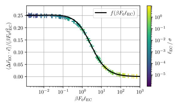
The function has the limiting behaviors for (in the limit of small EC lengths or weak propulsion forces) and for (in the limit of large EC lengths or strong propulsion forces). Figure 11 shows perfect agreement of the analytically calculated scaling function with the kEC simulation.
The limiting cases and differ in their behaviour under an opposing force (). For , the particle moves with probability the whole EC length against a weak opposing force resulting in (corrections from lifting and reflection are of order ), while for a move in the opposite direction . This leads to exactly the same behaviour as in a local MC algorithm for a local MC move of length in directions under the standard Metropolis rule fulfilling detailed balance, thus establishing equivalence to local Metropolis MC in the limit of small EC lengths . After expanding in and averaging over all directions this gives .
For , on the other hand, the particle is lifted after a short mean distance in direction against a strong opposing force and reflected. Essentially, this results in a move in the reflected direction over the whole EC length, . After averaging over all directions this gives resulting in .
In practice, the following fit function for is useful to interpolate between both limiting cases (see also Fig. 11):
| (19) |
with , , and , which is constructed to satisfy the limits for and for , so that is the only free parameter. This fit function can be used to speed up calculations in production runs.
I.3 Mean square and mean cubic ECMC move lengths for a single particle
Following similar steps, we can also calculate the mean square and mean cubic move lengths , and during one algorithmic ECMC step. In the following we use from Eq. (16).
I.3.1 The values of
If :
| (20) | ||||
| (21) |
If :
| (22) | ||||
| (23) |
The final result after averaging over the two cases and is
| (24) |
I.3.2 Derivation of
If :
| (25) | ||||
| (26) |
If :
| (27) | ||||
| (28) |
The final result after averaging over the two cases and is
| (29) |
We find both in the limits and , see also Fig. 12 (bottom, orange line).
I.3.3 Derivation of
If :
| (30) | |||
| (31) |
If :
| (32) | |||
| (33) |
using
| (34) | ||||
| (35) |
The final result after averaging over the two cases
| (36) |
II Validation of the kEC algorithm
II.1 One-body problem: the kEC algorithm becomes exact for small
We assign a kEC simulation time to each particle according to the relation for the first moment of the displacement in force direction, which holds exactly for single free ABPs by requiring that (see main text and preceding section). This procedure works equally well for all EC lengths as demonstrated in Fig. 11 and, thus, does not single out an optimal EC length. An optimal EC length could emerge if we also consider higher moments of the displacement in force direction as a function of and require that analytical results for ABPs also hold for the higher moments if we use for the displacement and for .
Simple exact analytical results for these higher moments for single free ABPs are not available, but approximate results which hold in the short time limit :
| (37) | ||||
| (38) | ||||
| (39) |
We have calculated the algorithmic counterpart of the left hand sides of Eqs. 37-39 in Sec. I.3 for one ECMC move analytically. Figure 12 shows , and as a function of the dimensionless parameter and demonstrates perfect agreement between these analytical calculations (orange lines) and kEC simulation data (black crosses). Note that all analytical results of Sec. I.3 only depend on the parameter .
It is not obvious whether or not Eqs. 37-39 for higher moments are valid within the kEC algorithm using the corresponding mean time per EC step . For this reason Fig. 12 also shows the right hand sides of Eqs. 37-39 for (blue lines). We expect the approximations in Eqs. 37 - 39 to break down for . This is equivalent to for high activity (and in the passive limit ), see main text. Numerically, we find the values of , at which the approximations in Eqs. 37-39 break down (= relative error of at least to the exact result), correspond - for all relevant active forces - to values of . In other words: the origin of the deviations in Fig. 12 between the blue and orange lines are not a result of the approximations in Eqs. 37-39 itself but are solely algorithmic for , i.e., due to a failure of our choice for a timestep.
Figure 12 shows that these algorithmic deviations between left hand and right hand sides of Eqs. 37-39 (orange and blue lines, respectively) become large for . For an optimal EC lengths , we would require left hand and right hand sides to exhibit a common intersection at a corresponding optimal -value. Since there are no common intersections, we are unable to determine a perfect EC length, which would reproduce all quantities related to the equations of motion correctly on a single particle level. However, in accordance with the observations made in the main text, all deviations in Fig. 12 vanish for small . This implies that all of those one-particle single-step quantities are correctly reproduced in the limit . More generally, we will derive that, for a single ABP, the kEC algorithm converges to the correct one-particle Fokker-Planck equation in the limit of vanishing EC lengths in the following section.
II.2 The one-particle Fokker-Planck equation for the kEC algorithm converges to the ABP Fokker-Planck equation for small
The stochastic motion of a single free ABP can be completely captured by the one-particle Fokker-Planck equation for the probability density to find the particle at position with orientation at time ,
| (40) |
In the following we will show that the kEC algorithm converges to the same one-particle Fokker-Planck equation in the limit of vanishing EC lengths or small timesteps . As a result, all moments of the displacement as a function of are correctly reproduced in this limit further generalizing the results of the previous sections.
Let be the probability density to find the particle at at time and the probability density to transition from to and from to within one step of the kEC algorithm with EC direction . The EC direction is given by the angle with the unit propulsion direction vector . We average over all angles , i.e., over all EC directions in each kEC step until time . The probability density one kEC timestep later can be related to via
| (41) |
where we average over all angles also in the last kEC step. The average time corresponding to one kEC step ; we will see in the course of our derivation of the Fokker-Planck equation how the algorithmic timestep has to be chosen to arrive at the ABP Fokker-Planck equation (40). Analogously to the standard derivation of Fokker-Planck equations, we can argue that the transition probability for a single kEC timestep is peaked around and, typically, for one kEC step. We will consider the limit of small and will neglect variations on scales . Therefore, we can expand in and around and to obtain
| (42) |
For our kEC algorithm the transition probability factorizes, because, after each ECMC move, the angular change is drawn from a Gaussian distribution with zero mean and and variance independently of the ECMC move vector. Therefore, there are no mixed terms in the Taylor expansion (42). We can specify the spatial transition probability as
| (43) |
for and
| (44) |
for with previously defined in Eq. (11). Therefore, the transition probability for a single kEC timestep is Gaussian in the angle and peaked around but, obviously, not Gaussian in due to the deterministic nature of EC moves. Nevertheless, also the above results for are peaked around for one kEC step as assumed in the Taylor expansion in Eq. (42).
The Taylor expansion in is justified if or . This is exactly the condition of smooth rotation discussed in the main text. If this condition is fulfilled we can also neglect higher orders of the Taylor expansion in because . Typically this is a relatively weak condition requiring only moderately small EC lengths for high activity . In Eq. (42), we also neglected higher orders of the Taylor expansion in because will be justified by the requirement of small EC lengths.
Further approximating and using
| (45) |
for the second moments of the ECMC move length (see Sec. I.3), we obtain
| (46) |
At this point, we see that the algorithmic timestep has to be chosen as
| (47) |
for the convective term to agree with the ABP Fokker-Planck equation (40). This is exactly our definition of the mean time from the main text. Finally, if also the diffusive term is required to agree with the ABP Fokker-Planck equation (40), we need
| (48) |
This poses a relatively strong condition and is only fulfilled for or small EC lengths . For , the apparent translational diffusion constant is larger than because is a decreasing function of . If the condition (48) is fulfilled, the one-particle Fokker-Planck equation of the kEC algorithm agrees with the ABP Fokker-Planck equation, assuring the validity of the kEC algorithm for single particles.
The strong condition can be weakened in practice because the diffusive term of the Fokker-Planck equation is only relevant for small time scales. There are three dynamic regimes for ABPs: (i) on time scales we find translation diffusion with ; (ii) on intermediate time scales below the persistence time, the ABP performs ballistic motion with ; (iii) on large time scales , the motion becomes a persistent random walk with . As a consequence, a violation of condition (48) will only give rise to a wrong translational diffusion constant that affects the short-time translational diffusion regime (i). The apparent diffusion constant is larger than and resulting in wrong results on time scales below the corresponding crossover time scale . As long as this erroneous behavior is limited to length scales , it will affect only small scale features of the distribution corresponding to variations below one particle diameter (or Fourier modes of the distribution with wave vectors ). This corresponds to small time scales , and as long as , only features of the distribution below the small scale are wrong. This condition can be written as resulting in the weaker condition
| (49) |
In the derivation of the Fokker-Planck equation we neglected variations of the distribution on scales , which remains consistent with neglecting variations on scales if the condition holds. Under this condition, we can also neglect higher orders of the Taylor expansion in in Eq. (42) because , which is also consistent with neglecting variations on scales . We conclude that we can increase up to order unity if we are not interested in features of the distribution below one particle diameter .
II.3 Two-body problem

Regarding the two-body problem, Fig. 13 presents a section of the heatmap of the absolute value of the relative deviation per grid element of the two-particle probability density between kEC and EDBD algorithms for and from the second configuration in Fig. 4 (). One may notice the relative errors of the grid elements in close proximity to the coordinate-fixed particle are seemingly higher than the ones further away. Assuming the EDBD algorithm to be correct, this may suggest that the kEC algorithm is not able to handle interactions between two particles completely correctly.
This objection, or at least its relevance, can be dismissed: Similar to the role of the displacement length for the kEC algorithm, the EDBD algorithm depends on a parameter (for further information on this subject see Ref. 22), whose choice influences the accuracy of the algorithm and is only exact in the limit of . As mentioned before, we cannot prove our algorithm to be exact, but presumably decreasing both and even further will lead to the deviations in proximity to the coordinate-fixed particle to shrink. If this is true, we can (in theory) tune both the deviations themselves as well as the length scales, on which they are relevant, at will. In practice this is of course limited to a certain degree since the required wall time increases, if the displacement length is reduced.
III Details on the time distribution in many-body simulations


As previously stated every particle has its own individual simulation time . This may cause problems - especially in a many-body simulation - because we would naively require that for all particles the exact same time has passed in order to maintain the correct propulsion directions (which are undergoing rotational diffusion with a persistence time ), which is a necessary condition to also preserve the order and causality of collisions (or interactions in general). However, in statistical physics, where we are interested in statistical averages and, typically, also averages over all particles (for densities of extensive observables), this is not necessary, and it appears to be sufficient if fluctuations in time do not cause uncontrollable statistical fluctuations of observables. There are three types of averages that we have to consider in any MC or molecular dynamics simulation: (1) Statistical averages of a quantity depending on a time difference can be obtained by taking averages over many samples of the system, each after the specified time difference . (2) Averages of a time-independent quantity can also be calculated as time averages over long time scales. (3) If is the density of an extensive quantity, we can average over all particles, in addition to sample averaging (1) or time averaging (2). We have to check for all three types of averages how they are affected by particles having slightly different, individual times in the kEC simulation technique. In particular, the approach (2) to take time averages has to be applied with care.
To control the errors of any sample, time, or particle average, we have to investigate the time distribution of particles for different EC lengths, timescales, system sizes, and different phases of the system such as the dense MIPS phase or a dilute phase. We focus on two systems of particles in different parameter regimes: (i) a dilute system (), where MIPS does not occur, and (ii) a dense system (), where MIPS does occur. Exemplary snapshots can be found in Fig. 14.
First of all, we want to investigate the distribution of passed times of the particles in the dense system snapshot just mentioned. In Fig. 15 one can find the particles color-coded with respect to their individual time. It is worth noting in the case MIPS occurs one cannot find a systematic difference between the individual times of the particles in the dilute phase and the dense one. This is significant, as it proves the same time passes in the entire system regardless of the local density.
In Fig. 16, we show the distributions of particle times on short timescales (mean time per particle ): regardless of whether MIPS occurs the time distributions that are measured using large EC lengths are rather wide and everything but sharp. Additionally one can observe multiple equidistant maxima, separated by the mean time per EC step . These maxima appear particularly in the dilute phase, if no collisions and subsequent lifting moves take place during one EC move, which results in the total time being assigned to each single particle move according to Eq. (6). Reducing the EC length leads to an increase in the number of maxima. The reason for this is related to the non-linear relationship between and the EC length. By decreasing the mean time per EC step also gets smaller and therefore the number of EC steps per time interval increases. This implies that each particle is at least on average more often the starting point of a new EC step and due to the increase of the total displacement length more lifting moves take place. Consequently both the relative and absolute height of each peak shrinks. Because collisions (and therefore lifting moves) are in general way more frequent in a dense system, smooth shapes of the time distribution are reached for larger EC lengths as it is less probable to assign to a single particle. Finally, reducing the EC length even further leads to bell-shaped time distributions, centered around the mean time per particle , whose standard deviation appears to follow a power law with an exponent . The shape of these distributions is in some way to be expected, as we anticipate the total displacement length of each particle and therefore also the individual time to be approximately the same if the total number of EC steps and therefore the total displacement length is large.
Concerning medium () and long () timescales (see Fig. 17), we notice - regardless of the particle density - the relative and absolute values of the equidistant peaks separated by the mean time per EC step to decrease steadily by increasing the mean time per particle . This appears to be a rather fast process, as the maxima are barely visible already at . Additionally and similar to reducing the EC length , a growing mean time per particle leads to the time distribution to become bell-shaped. Furthermore the relative standard deviation that corresponds to the visible width in the plots in Fig. 17, decreases as a power law as increases, implying the individual times of the particles are converging relatively.
Based on these observations, we investigate the relationship between the mean time per particle and the standard deviation of the time distribution and the influence of both the number of particles as well as the EC length for the dense system and . Fig. 18 reveals the standard deviation of the time distribution to be proportional to the square root of the mean time per particle, . Additionally one may notice to initially increase with , reach an EC length dependent peak ( for , for and for ) and afterwards to drop slightly, settle and thus become independent of . We find
| (50) |
with only weakly depending on and the exponent of ranging from for to for .
As mentioned before we require the individual particle times to roughly coincide, which can be quantified by the loosely defined criterion , which assures that particles remain within one persistence time, i.e., the propulsion directions will not be affected by the time spread. For , the standard deviation satisfies at and clearly fulfills this criterion. This implies further that we can simulate the system for several thousand persistence times using the kEC algorithm with without ever violating the criterion.
The result (50) enables us to discuss the three types of statistical averages mentioned in the beginning of the section systematically: First, we notice that a width of the time distribution also implies measurement errors of an observable after a time . (1) Averages over samples of a time-dependent quantity are based on the fact that the mean over samples has an error , which can be controlled by the sample number as long as samples are statistically independent. The result of the additional time distribution of particles in the kEC simulation is simply that we have to average over more samples for larger to reduce the error of the mean. (2) Time averages over times of a time-independent quantity in intervals that should be larger than one autocorrelation time of the system have to be treated with more care because errors grow in time according to Eq. (50). Therefore, the error of such a time average is no longer reducing as usual, but actually saturating to an -independent value. (3) Averages over all particles will still be effective and reducing the error of the average because is essentially -independent according to Eq. (50).
Taking all of these information into account, our algorithm appears to be suitable to deal with many-body simulations. One can simply decrease the displacement length to align the individual particle times, both their relative and also absolute values. This allow us to satisfy the condition for very long simulation times. Typically, we only need simulation times of persistence times to reach stationary states (in case of ) and observe phenomena such as MIPS. Therefore we can set up the kEC algorithm in a way that for every particle (almost) the exact same time passes. This is true regardless of the presence of MIPS. Moreover, averaging over many samples or over particles are still effective ways to reduce errors of mean values. Only time averages have to be treated with care as errors of mean values saturate (with respect to the number of samples). Errors of all averages, including time averages, can be controlled by shrinking . To avoid confusion, it should be emphasized that statistical averages - solely taking the time distribution into account - can only converge to correct values in the limit . For large displacement lengths some of the mean values are converging, but to values related to distorted dynamics.
IV Derivation of the -body Fokker-Planck equation in the dilute limit
In order to prove our kEC algorithm also to be exact for general -body problem there are two problems, which one needs to overcome: (1) different individual times as a consequence of the time distribution and (2) complex algorithmic dynamics due to lifting moves. While we are currently not able to handle the second problem, one can ignore this issue in the dilute limit . Admittedly, the system does not exhibit interesting physical phenomena such as MIPS in a pure dilute state. Nevertheless, we still want to explore this limit, because one may argue, if our algorithm is correct for the dilute -body system it does not become discontinuously incorrect, if the packing fraction is increased to finite values.
Before dealing with the -body Fokker-Planck equation itself, we need to make sure the exact same time passes for every particle. Let us say, we want our system to evolve for the time interval (). For a given EC length, we would require EC steps for a single particle to satisfy
| (51) |
and therefore steps so that for each particle the time evolves on average by . After steps, the time distribution of the entire system - as demonstrated in the previous section - would be a Gaussian. We expect the standard deviation of the time distribution to shrink if one reduces the EC length, similar to the configuration we discussed in Sec. III. In other words: automatically leads to . However, a Gaussian distribution with vanishing standard deviation is a -distribution
| (52) |
This way, we can make sure that all individual particle times are exactly the same.
Let be the probability density of the dilute (non-interacting) -body system. In the limit all individual times are the same and holds. To find the -body Fokker-Planck equation we need to find an expression for . In Sec. II.2 we found
| (53) |
We can use this formula iteratively and ignore all terms smaller than , which leads to
| (54) |
In the dilute (non-interacting) limit all coordinates are completely independent of each other. This allows us to employ the same procedure, we just used for a single ABP, to obtain
| (55) |
This can easily be transformed to
| (56) |
which we identify as the correct -body Fokker-Planck equation of non-interacting ABPs.
V Details of the kEC simulations for the phase diagram of hard disks
To construct the large phase diagram in Fig. 6 in the main text, we simulate particles using in a square box with area and periodic boundary conditions. We change the global packing fraction by changing the system size at a fixed particle number. Depending on the Péclet number and the global packing density, the phase behavior is classified and the binodal is determined.
V.1 Calculating the distribution of the local packing fraction

The investigation of the MIPS phase and its stability is performed via calculating the probability density distribution of the local packing fraction, see Fig. 19. In order to calculate this quantity, we first divide the simulation volume into multiple subvolumes, each of which has the area . We calculate the local density in each of those subvolumes and (by averaging over many snapshots) use this data to construct the probability density distribution of the local packing fraction.

V.2 Determination of binodal and spinodal lines
To determine the binodal line, we calculate the probability density distribution of the local packing fraction. If MIPS occurs, exhibits two distinct maxima corresponding to the dilute and dense phase (see Fig. 19). The binodal lines indicate the coexisting densities and are determined by averaging the coexisting densities (the positions of the two maxima of ) for different global packing fractions at the same Péclet number.
Orange points in Fig. 6 of the main text, which lie within the region spanned by the binodal line, correspond to global packing fractions, where the homogeneous initial state is only metastable. They should become unstable to MIPS by strong perturbations, such as strong density fluctuations. To check this, some systems are simulated with , similar to Ref. 22, with an already phase-separated initial state, which we prepared by placing a dense and approximately square-shaped particle cluster in the center of the system. In addition, all initial driving forces are aligned in the direction of the system center. The results are shown in Fig. 20, where red circles represent systems with phase separated final states (see insets). We find that the phase separated state is globally stable, while the homogeneous state is only metastable, for most of the orange points, which lie between the coexistence lines. Small deviations, especially near the binodal, are due to finite-size effects cf. to a free energy barrier of homogeneous nucleation.
The method to calculate the binodal lines, which was previously explained, does not work close to the critical point. This is because in proximity of one cannot determine the peaks related to the dilute and dense phase, as they are barely set apart from the rest of the distribution and become virtually indistinguishable from small fluctuations of . Of course one can deal with these problems by increasing the sample and system size, which would lead to an increase of the overall computational effort.
VI Handling of non-periodic boundary conditions and external potentials
Throughout this work we have focused on periodic boundary conditions, however certain problems require non-periodicity via soft or hard walls. Since soft walls can be viewed as short-ranged external potentials and hard walls are the infinitely steep limit of the former, we will briefly address how to incorporate external one-particle potentials into our algorithm.
Before dealing with the kEC algorithm, we should take a closer look at the dynamics of the new setup. In the presence of an external potential the equation of motion for an isolated particle takes the form
| (57) |
which leads - in the limit of small timesteps - to the mean displacement
| (58) |
As mentioned in the beginning, a rejection caused by an external potential leads to a reflection of the displacement direction at the potentials equipotential surface. There are two possibilities of adjusting the mean time per EC move for an active particle: One could either calculate the mean move vector during one ECMC step for an algorithm that handles the active force and external potential separately, or we consider an algorithm that combines both active and external force into one potential. The first option keeps up the idea that each interaction can be handled entirely independently in the ECMC algorithm through factorization of the Metropolis filter, but it is also way more complicated to calculate for such a factorized version of the algorithm. Therefore, we strongly suggest to use the second option. As the previous analysis proved, the dynamics of a single free ABP is correct in the limit . As we expect the same to be true in the presence of an external potential, we can approximate any potential during a single EC step as a linear potential (this is the same idea as the assumption of small timesteps in Eq. (58)). This allows us to calculate analogously to Sec. I.2 using the combined total force instead of and instead of . In case of short-ranged potentials and/or nonlinear potentials this procedure causes the mean time per EC step to depend on the position of the particle . This may raise the concern, that the individual particle times may vary greatly. However, because of the shape of the time function we expect the particle times to coincide at least in the limit and therefore the limit of vanishing EC lengths.