Generic Hölder level sets and fractal conductivity Thanks: ∗
The project leading to this application has received funding from the European Research Council (ERC) under the European Union’s Horizon 2020 research and innovation programme (grant agreement No. 741420).
This author was also supported by the Hungarian National Research, Development and Innovation Office–NKFIH, Grant 124003 and at the time of completion of this paper was holding a visiting researcher position
at the Rényi Institute.
Thanks: This author was supported by the ÚNKP-21-3 New National Excellence of the Hungarian Ministry of Human Capacities, and by the Hungarian National Research, Development and Innovation Office-NKFIH, Grant 124749.Thanks: This author was supported by the ÚNKP-20-3 New National Excellence Program of the Ministry for Innovation and Technology from the source of the National Research, Development and Innovation Fund, and by the Hungarian National Research, Development and Innovation Office–NKFIH, Grant 124749.
Mathematics Subject
Classification: Primary : 28A78, Secondary : 26B35, 28A80, 76N99.
Keywords: Hölder continuous function, level set, Sierpiński triangle, fractal conductivity, ramification.
Abstract.
Hausdorff dimensions of level sets of generic continuous functions defined on fractals
can give information about the “thickness/narrow cross-sections” of a “network” corresponding to a fractal set, .
This lead to the definition of the topological Hausdorff dimension of fractals.
In this paper we continue our study of the level sets of generic -Hölder- functions. While in a previous paper we gave the initial definitions and established some properties of these generic level sets, in this paper we provide
numerical estimates in the case of the Sierpiński triangle. These calculations give better insight and illustrate why can one think of these generic -Hölder-
level sets as something measuring “thickness/narrow cross-sections/conductivity”
of a fractal “network”.
We also give an example for the phenomenon which we call phase transition for . This roughly means that for a certain lower range of s only the geometry
of determines while for larger values the Hölder exponent, also matters.
1. Introduction
In [7] the concept of topological Hausdorff dimension was introduced. It has turned out that this concept was related to some “conductivity/narrowest cross-section” properties of fractal sets and hence was mentioned and used in Physics papers, see for example [1], [2], [3], [4], and [5]. In [15] the authors studied topological Hausdorff dimension of fractal squares.
The starting point of the research leading to the definition of topological Hausdorff dimension was a purely theoretic question concerning the Hausdorff dimension of the level sets of generic continuous functions defined on fractals, apart from [7] see also [6]. (Some people prefer to use the term typical in the Baire category sense instead of generic.) It has turned out that these generic level sets “can find” the narrowest cross-sections” of the fractals on which they are defined. For example the Sierpiński triangle has many zero dimensional “cross-sections” and the Sierpiński carpet has many dimensional cross sections. These are the values of the Hausdorff dimensions of the level sets for almost every levels in the range of the generic continuous functions defined on them. On Figure 1 the red lines crossing the Sierpiński carpet are intersecting the fractal in dimensional sets. In case of the Sierpiński triangle near the red lines one can obtain curves intersecting the fractal in finitely many points.

The level sets of generic continuous functions are “infinitely compressible” which informally speaking means that we can squeeze almost every level in the range of the continuous function to places where the fractal domain is the “thinnest”, yielding that the dimension of these level sets are small. Consider the Sierpiński triangle for example: even though one cannot squeeze almost every level set onto a curve which intersects the triangle in a countable set of points, for a generic continuous function almost every level set stays “near” such curves, yielding that they have zero dimension. It is a natural question what happens if the level sets/regions of our functions are not “infinitely compressible” and hence due to thickness of the level regions we cannot use for almost every levels the parts of our fractal domains where they are the “thinnest”. The simplest way to impose a bound on compressibility is considering Hölder functions instead of arbitrary continuous functions. More specifically and explicitly, it is straightforward to observe the level sets of generic 1-Hölder- functions. In our recent paper [9] we started to deal with this question.
|n Section 2 we give and recall some definitions and theorems from [9] and prove some preliminary results. Out of these definitions we mention here that denotes the essential supremum of the Hausdorff dimensions of the level sets of a generic -Hölder- function defined on . In [9] we showed that if , then for connected self-similar sets, like the Sierpiński triangle equals the Hausdorff dimension of almost every level-set in the range of a generic 1-Hölder- function, that is, it is not necessary to consider the essential supremum.
In Sections 3 and 4 we consider -Hölder- functions defined on the Sierpiński triangle, . In Theorem 3.2 we obtain a lower estimate for which equals in this case the Hausdorff dimension of almost every level-set of any 1-Hölder- function defined on .

In Theorem 4.5 for the Hausdorff dimension of almost every level-set of a generic 1-Hölder- function we also calculate an upper estimate. Level sets of 1-Hölder- functions can get quite complicated. In some very special cases when either the function is linear, or there is a direction such that it is constant on lines pointing in this direction we need to consider intersections of these lines with our fractal. Intersection of fractals with lines is a classical topic (see for example [16]), which even in the case of the Sierpiński triangle, or carpet is still subject of more recent research as well, see [8] [14].
In Section 5 we show that if our fractal is a self-similar set satisfying the strong separation condition then the Hausdorff dimension of almost every level-set of a generic 1-Hölder- function is constant zero for all , that is the introduction of generic 1-Hölder- functions is not giving any new information compared to the case of continuous functions.
In Section 6 we discuss and illustrate a phenomenon which we call phase transition. In Theorem 6.1 we give an example of a fractal for which the Hausdorff dimension of almost every level-set of a generic 1-Hölder- function for small values equals the Hausdorff dimension of almost every level-set of a generic continuous function defined on . This means, at a heuristic level, that for such fractals the level sets of generic 1-Hölder- functions are as flexible/compressible as those of a continuous function. On the other hand, for larger values of we have , that is after a critical value of these level sets are not as flexible/compressible as those of a continuous function and we experience some “traffic” jams as we try to push across the fractal the level sets of generic 1-Hölder- functions. The fractal discussed in this section will be the Cartesian product of a fat Cantor set with itself, hence it will be of zero topological dimension. Note that due to Section 5, such a construction requires fat Cantor sets. Indeed, a self-similar Cantor set cannot have the above properties. In [9] we proved that is monotone increasing in for any compact set . It is a natural question whether this function is continuous. For the fractal of Theorem 6.1 there is not only a phase transition at , but also a jump discontinuity of . In [9] we give an example of a fractal for which has a jump discontinuity at and for that fractal there is no phase transition. The behaviour exhibited by these fractals is in contrast with the behaviour of the Sierpiński triangle : as demonstrated by the bounds given in Section 3 and 4, is continuous and increasing in 0, ruling out the possibility of phase transition.
2. Preliminaries
In this section first we recall some definitions and results from [9].
The distance of is denoted by . If then the diameter of is denoted by The open ball of radius centered at is denoted by .
Assume that for some . In what follows, will be some fractal set, usually we suppose that it is compact.
We say that a function is -Hölder- for and if for all . The space of such functions will be denoted by , or if is fixed then by . The space of Hölder- functions will be denoted by , that is We say that is -Hölder- if there exists such that is -Hölder-. The set of such functions is denoted by , that is .
In order to introduce topology on the set , we think of it as a subset of continuous functions equipped with the supremum norm To obtain a closed subset of , we take -Hölder- functions, , and use the metric coming from the supremum norm.
For and we denote by the open ball of radius centered at , the ball taken in the supremum norm. If then will denote the corresponding open ball in the subspace
Since similarities are not changing the geometry of a fractal set to avoid some unnecessary technical difficulties we suppose that we work with fractal sets of diameter at most one (unless otherwise stated). This way
| (2.1) |
Suppose . Given the sets , if for all and .
The -dimensional Hausdorff measure (see its definition for example in [10]) is denoted by . Recall that the Hausdorff dimension of is given by
| (2.2) |
We will use the Mass Distribution Principle, see for example [10], Chapter 4.
Theorem 2.1.
Let be a mass distribution (a finite, non-zero Borel measure) on . Suppose that for some there are numbers and such that for all sets with . Then and
Let for any function , that is denotes the Hausdorff dimension of the function at level .
We are interested in the Hausdorff dimension of the level sets for sufficiently large sets of levels in the sense of Lebesgue. Hence we put
where denotes the one-dimensional Lebesgue measure.
The definition of depends on . In case we want a definition depending only on the fractal we can first take
where the locally non-constant property is understood as is non-constant on where is any neighborhood of any accumulation point of .
As we are only concerned with nonnegative numbers, by convention the infimum of the empty set is . The value concerns those functions for which “most” level sets are smallest possible.
We denote by , or by simply the set of dense sets in .
We put
| (2.3) |
We recall Theorem 5.2 of [9], which states that one can think of in a substantially simplified form, essentially due to the supremum being a maximum, for which the infimum is taken over a singleton. Precisely:
Theorem 2.2.
If and is compact, then there is a dense subset of such that for every we have .
As we mentioned in the introduction, another result from [9] implies that if and is a connected self-similar set then one can think of as the Hausdorff dimension of almost every level set in the range of a generic function.
To include generic continuous functions in our notation we set
where is the topological Hausdorff dimension of . For the definition see [7]. By results in [7] we have that if is a generic continuous function on , then
For brevity, often we will omit from our notation.
Recall from [9] the following trivial upper bound for .
Theorem 2.3.
For any bounded measurable set , we have
(As usual, denotes the upper box dimension of .)
In [9] we state and prove several approximation results. We will use the next two lemmas later in this paper.
Lemma 2.4.
Assume that is compact and is fixed. Then the Lipschitz -Hölder- functions defined on form a dense subset of the -Hölder- functions. (We say that is Lipschitz -Hölder-, if is Lipschitz and .)
Lemma 2.5.
Assume that is compact, , and are fixed. Then the locally non-constant piecewise affine -Hölder- functions defined on form a dense subset of the -Hölder- functions.
3. Lower estimate for arbitrary functions on the Sierpiński triangle
In this section as an example we consider the Sierpiński triangle, . It is a connected self-similar set. Hence by a result of [9] equals the Hausdorff dimension of almost every level-set of a generic 1-Hölder- function.
Some people prefer to work with different versions of the Sierpiński triangle. We work with the one which is obtained by starting with an equilateral triangle of side length one. Hence it satisfies our earlier assumptions about the fractals considered since its diameter equals one. Its topological Hausdorff dimension equals one and this implies that for a generic continuous function every level set is zero-dimensional, see [7]. The level sets of continuous functions are very flexible, and very “compressible”, hence during the proof of this theorem one can capitalize on the fact that the Sierpiński triangle is very “thin” near the vertices of the small triangles appearing during its construction. As Hölder- functions do not have this flexibility, one can expect that their level sets generically exhibit a different behaviour. In Theorem 3.2 we obtain a lower bound for the Hausdorff dimension of almost every level set in the range of an arbitrary 1-Hölder- function defined on . This lower estimate is positive for . In Theorem 4.5 we give an upper estimate for the Hausdorff dimension of almost every level set of the generic 1-Hölder- function defined on , that is we estimate from above. Both the lower and upper estimates tend to as . Of course, it would be interesting to determine the exact value of the function , but this seems to be quite difficult.
By its definition the Sierpiński triangle is expressible as where is the union of the triangles appearing at the th step of the construction. The set of triangles on the th level is . For we denote by the set of its vertices. Moreover, let be the set of the points which are vertices of some , and their union is . We are interested in the Hausdorff dimension of the level sets of a 1-Hölder- function for .

Suppose . It will be useful for us to define the self-similar set as well. It is induced by the similarities which map to any triangle on the boundary of . For example, , while the case is shown by Figure 3 where the shaded triangles on the sides of are used in the definition of . (The lighter shaded triangles will have importance later.)
One can easily check that the number of triangles used in the construction of is , and the th level of consists of certain triangles of . Let us denote the family of these triangles by , the union of their vertices for fixed by , and the union of vertices for all the triangles in some by . It is clear that a 1-Hölder- function restricted to is still a 1-Hölder- function.
Suppose that is a 1-Hölder- function and . We can define the th approximation of denoted by for any and as the union of some triangles in . More explicitly, is taken into if and only if has vertices and such that , that is, is in the interior of the convex hull . The idea is that in this case necessarily intersects . On Figure 3 the level set corresponding to is the intersection of the red curve with . The set consists of the light shaded triangles. Now it is easy to check that, using the notation for the convex hull,
| (3.1) |
hence if contains a triangle then contains a triangle such that . We introduce the following terminology: we say that is the -descendant of if there exists a sequence of triangles such that and for . We denote the set of -descendants of by .
Observe the obvious property that for any we can label the vertices in such that . We refer to as the extreme vertices of . Since we supposed that we have . If then we call only one vertex as an extreme vertex, the other vertex denoted by will not regarded to be an extreme vertex. We proceed analogously if .
We define the conductivity of any triangle inductively (as is fixed during most of our arguments, it will be omitted from the notation unless it might cause ambiguity). If , we define . On the other hand, if , there is a unique triangle such that . Now if is one of the two triangles at an extreme vertex of , then let (in this case we say that is an extreme triangle of ), while in any other case we let . The following lemma can be thought of as the weak conservation of conductivity:
Lemma 3.1.
Assume that and . Then we have
Proof.
By induction, it suffices to work with . Consider the vertices and on which is minimal and maximal respectively in . Since and there are at least two edges of containing points of . One of them is the one connecting and .
If there is a which contains all the intersection points of the edges of and then it should contain , or . Hence, it is an extreme triangle of and the conductivity of equals that of .
Otherwise we have at least two triangles of which are in and the sum of their conductivity is at least the conductivity of . ∎
Now we have enough tools to turn our attention to the Hausdorff dimension of the level sets of a 1-Hölder- function .
Theorem 3.2.
Assume that is a 1-Hölder- function for some . Then for Lebesgue almost every we have
| (3.2) |
Proof of Theorem 3.2.
Since is compact and connected is a closed interval. Moreover as is a countable and dense subset of the set is countable and dense in . Suppose that . Then we can find such that . Due to self-similarity properties, we can assume .
Restrict to some . The number will be fixed later, it is useful to think of it as something large. Roughly speaking, in order to bound the dimension, we would like to obtain that for Lebesgue almost every we have that does not intersect triangles with high conductivity on the th level for large . Consequently, by Lemma 3.1 we could deduce that intersects “many” triangles, which yields “high” Hausdorff dimension due to the Mass Distribution Principle (Theorem 2.1). In order to formalize this idea, we would like to estimate the number of triangles with high conductivity.
For any we can consider the chain of triangles such that and . We bound from above the number of triangles in , whose conductivity is at least , where is chosen to be a small rational number, hence is an integer for infinitely many . From this point on we restrict our arguments to such s, that is we suppose that for some where . The conductivity is at least if is an extreme triangle for at least of the indices .
The number of such triangles is estimated from above by
as we can choose the places where we use one of the two extreme triangles, and in the remaining places we allow the usage of any of the triangles, hence giving an upper bound. By standard bounds on binomial coefficients, this can be estimated from above by
| (3.3) |
The diameter of the triangles in is . Consequently, due to being 1-Hölder- and by (3.3), we know that the -image of the union of the well conducting triangles has Lebesgue measure at most
| (3.4) |
Assume that . Then the corresponding series is convergent, hence we can apply the Borel–Cantelli lemma to deduce that almost every appears in the image of well conducting triangles only on finitely many levels. Consequently, for almost every , if is large enough, must intersect at least triangles of , as the sum of the conductivities of triangles in for which , is at least 1. We will use this observation paired with the Mass Distribution Principle, Theorem 2.1 to give a lower bound on the dimension of almost every level set, but first, let us consider the question how to choose in order to guarantee that . Elaborating (3.4), we would like to assure
| (3.5) |
If this inequality holds for instead of , that is still fine for our purposes. Rewriting our powers in base , it leads to
that is after taking logarithm
We clearly need to satisfy this inequality, as only the third term can be negative. Fixing this assumption, after rearrangement we obtain that it holds if and only if
| (3.6) |
No matter how we fix the rational number , such an implies . We notice that can be chosen arbitrarily close to , and due to the continuity of the left hand side of (3.6), if they are sufficiently close to each other, then we can choose so that
| (3.7) |
We recall that for such we have that for almost every , if is large enough, can only intersect triangles of with conductivity smaller than . Fix such an and consider only such large enough s. We define a probability measure on .
Due to Kolmogorov’s extension theorem (see for example [17], [18] or [13]) it suffices to define consistently for any triangle in . First, if is not an -descendant of , let . For descendants, we proceed by recursion. Notably, if is an -descendant in , and is already defined, then we divide its measure among its -descendants in proportionally to their conductivity. More explicitly, for an -descendant of we define
Then using Lemma 3.1 by induction it is clear that
Hence,
| (3.8) |
Next we want to use the Mass Distribution Principle. Recall that we assumed that we work with s of the form . Now assume that we have a Borel set such that for its diameter we have . By a simple geometric argument one can show that might intersect at most triangles in for some constant not depending on . (One can consider the triangular lattice formed by triangles with side length and it is easy to see that a Borel set with diameter can intersect only a limited number of the triangles.) Consequently, the number of -descendants of in intersected by is also bounded by . For such an -descendant we can apply (3.8), hence
As , the mass distribution principle tells us that if there exists independent of with
then . Such a exists if and only if
Hence the expression on the right hand side of this inequality is a good choice for in the mass distribution principle, thus it is a lower estimate for for any valid pair . Using (3.7) and the argument leading to it, we can approximate by possible s and for sufficiently good approximations we can use
Consequently,
∎
4. Upper estimate of for generic functions
Definition 4.1.
We say that is a piecewise affine function at level on the Sierpiński triangle if it is affine on any .
If a piecewise affine function at level on the Sierpiński triangle satisfies the property that for any one can always find two vertices of where takes the same value, then we say that is a standard piecewise affine function at level on the Sierpiński triangle.
A function is a strongly piecewise affine function on the Sierpiński triangle if there is an such that it is a piecewise affine function at level .
Here we state a specialized version of Lemma 2.5 valid for the Sierpiński triangle.
Lemma 4.2.
Assume that , and are fixed. Then the locally non-constant standard strongly piecewise affine -Hölder- functions defined on form a dense subset of the -Hölder- functions.
Before proving this lemma we need to state and prove another one.
Recall that .
Lemma 4.3.
Suppose, , , , is Lipschitz- and -Hölder- on . Then there exists such that for any fixed if for any is -Hölder- on and for all then
| (4.1) |
Proof.
Since is -Hölder- on we can choose such that is -Hölder- on .
If
then
Choose .
First we prove that is -Hölder-.
Suppose that , , and and select vertices
| (4.2) | and . |
Then by our assumption and . Since the diameter of and equals we obtain
where the convergence is uniform due to being separated from zero. Thus, we can choose large enough (independently of and ) such that
| (4.3) |
Suppose . If then by our assumption
| (4.4) |
If , but and has a common vertex then by geometric properties of the Sierpiński triangle , hence by the Law of sines
and similarly . Hence,
| (4.5) |
If and does not have a common vertex then . Choose and . Then
Thus
| (4.6) |
Proof of Lemma 4.2 .
With a rather straightforward modification of the proof of Lemma 2.5 one can verify the following weaker form of Lemma 4.2: locally non-constant strongly piecewise affine -Hölder- functions defined on form a dense subset of the -Hölder- functions.
Hence suppose that and are given. By the previous remark choose a locally non-constant and such that
| (4.7) |
By our assumption about the diameter of , the triangles in are of side length .
Since is piecewise affine on any it is Lipschitz- for a suitable and -Hölder- on By Lemma 4.3 used with and instead of and choose .
We want to obtain a locally non-constant standard strongly piecewise affine -Hölder- function which is -close to . Since is a locally non-constant strongly piecewise affine -Hölder- function which is -close to we will modify to obtain , -close to .
Select a sufficiently large which satisfies
| (4.8) |
To obtain we will modify on the triangles . On the functions and will coincide.
Suppose that is arbitrary. Denote its vertices by and . Suppose that and are the midpoints of the segments , and , respectively. We denote by , and the triangles , and , respectively. The triangles , belong to .
We define , and . We also assume that is affine on any triangle .
By our choice of we have
Suppose that (a similar argument works for the triangles and ). Denote by the orthogonal projection onto the second coordinate “”-axis then
where at the last step we used (4.8). Hence if Lemma 4.3 is applied with the constants fixed above to the function as , we obtain a standard strongly piecewise affine -Hölder- function which is -close to . ∎
We denote by the rescaled and translated copy of in a way that the vertices of are , and .
It is clear that can be tiled by translated copies of the triangle and its mirror image about the -axis. We denote the system of these triangles by . For we also use the scaled copies of this triangular tiling consisting of triangles of the form , . The system of triangles belonging to this tiling is denoted by . During the definition of box dimension many different concepts can be used, see for example [10]. Given a set we denote by the number of those triangles which intersect . It is an easy exercise to see that
| (4.9) |
Lemma 4.4.
Suppose . There exists , such that , and there exists an exceptional set such that and for any
| (4.10) |
Since the lower, and hence the upper box dimension is never less than the Hausdorff dimension we also have
| (4.11) |
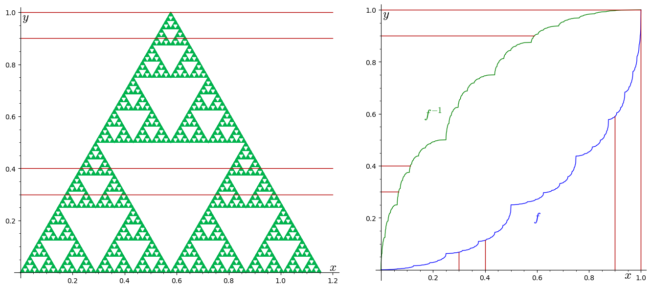
Proof.
The basic concepts and results of ergodic theory we use in the sequel can be found for example in [12]. Suppose that . Denote by the doubling map on , that is , where , denotes the fractional part. Denote by , the invariant ergodic measure for which
| (4.12) |
Set . Suppose that , and , . By (4.12) any interval of the form is of measure at most . Since can be covered by no more than three such intervals we have
| (4.13) |
Since is ergodic with respect to by the Birkhoff Ergodic Theorem (see for example Chapter 4 of [12]) we have for almost every
| (4.14) |
(where denotes the th digit after the binary point in the binary representation of ). We denote by the set of s satisfying (4.14). Since for any , we have and the intervals generate the Borel sigma algebra we have for any Borel set . Hence and for almost every we have
For set and select such that . From (4.13) it follows that is a -Hölder- function.
The definition of the Sierpiński triangle implies that if is not a dyadic rational then the horizontal line
| (4.15) | intersects many triangles of . |
If needed, by removing a countable set we can assume that does not contain dyadic rational numbers. Set . If then and (4.10) is obvious. If then by (4.14) and (4.15) we have
| (4.16) |
∎
Theorem 4.5.
For any , we have .
In the proof we will use the following Corollary of Lemma 5.1 from [9]:
Lemma 4.6.
Suppose that , is compact. If is a countable dense subset of , then there is a dense subset of such that
| (4.17) |
Proof of Theorem 4.5.
Suppose that consists of locally non-constant standard strongly piecewise affine -Hölder- functions defined on , and this set is dense in the space of -Hölder- functions defined on . It is also clear that each is Lipschitz with a constant which we denote by .
We suppose that is selected in a way that is piecewise affine on each and there exist such that
| (4.18) | and if denotes the third vertex of |
| then . |
Observe that if we take subdivisions, that is we take an then (4.18) holds for suitably chosen vertices of triangles . Later in the proof we will select a sufficiently large .
Next we define a function satisfying
| (4.19) |
First using Lemma 4.3 with , , , and , select .
We define such that with
| (4.20) |
Since is -Lipschitz if , are different then and
| (4.21) |
if we suppose that is chosen large enough to satisfy
| (4.22) |
Suppose that . For ease of notation we will write instead of for Using notation from the second paragraph before Lemma 4.4, denote by the similarity for which and the vertices of for which we have (4.18) satisfied are mapped in a way that
| (4.23) | for |
Then for every
| (4.24) |
Let be given by Lemma 4.4. For we put
| (4.25) |
Suppose then
| (4.26) |
where at the last step we used (4.22).
Since consists of finitely many triangles , finite union of exceptional sets of measure zero is still of measure zero, and affine transformations are not changing the Hausdorff dimension we obtain from (4.11) and (4.25) that for almost every and for every . Therefore for every and by the density of the functions and (4.19) the functions are also dense in . Hence we can apply Lemma 4.6 with the compact set and the dense set of functions to obtain a dense set such that for any . Since in (2.3) there is also a supremum a little extra care is needed. Using Theorem 2.2 select and denote by a dense subset of such that for every we have . Since is non-empty we can select a function from it. For this function This completes the proof of the theorem. ∎
For from Theorem 2.3 one can obtain that Since this upper estimate is worse.
5. Strongly separated fractals
In this section, our goal is to prove that vanishes for small in the case when admits a strongly separated structure in the following sense:
Definition 5.1.
For some , a nonempty set admits a separated structure, if there exists , and a sequence of finite families such that
- •
for each ,
- •
for any and we have ,
- •
for any and distinct we have .
As the next lemma shows such fractals are quite common. For the well-known definitions of iterated function systems and the strong separation condition we refer to standard textbooks on fractal geometry like [10].
Lemma 5.2.
Assume that is an iterated function system satisfying the strong separation condition. Moreover, assume that each is bi-Lipschitz, that is for there exists with
Then the attractor of the system admits a separated structure for some .
More specifically, if each is a similarity, that is is a self-similar set, then admits a separated structure for some .
Proof.
For any we say that is a th level cylinder of .
First we show that is a valid choice. To establish this, we will define the required families for any by considering smartly chosen cylinder sets. Notably, will consist of cylinders such that for the diameter of any of them,
| (5.1) |
This condition is clearly satisfiable by iteratively splitting the cylinders we consider. In particular, start this procedure with the -level cylinder , split it into many first level cylinders. Later on, in each step split precisely those cylinders which have diameter larger than , and leave the others unchanged. Due to the bi-Lipschitz property of each , this algorithm produces a finite system of cylinders in finitely many steps, such that each cylinder satisfies (5.1). It yields that the above choice of is valid indeed for large enough .
Assume now that the minimal distance between any two of the sets is , and consider arbitrary cylinders . Now let be the smallest cylinder set containing both and . In this case, , where is the composition of a finite sequence of functions for some . Consequently, and for some . It yields that the distance between and is at least as large as the distance between and . Moreover, has diameter at least : otherwise it would not have been splitted during the procedure creating . Hence if , we can deduce that for the number of functions determining we have
That is for
Altogether it yields that as the distance between and is at least , the distance between and is at least
which implies that is a valid choice for with a large enough , concluding the proof of the first part.
Concerning the statement for self-similar sets, capitalizing on the fact that is a similarity, we are able to take a more comfortable route to conclude the proof from the observation that has diameter at least . Notably, this implies that the similarity ratio of is at least , and consequently, the distance between and cannot be smaller than . It verifies that in this case can be chosen. ∎
The essence of this section is the following lemma:
Lemma 5.3.
Assume that admits a separated structure, and . Then piecewise constant functions with finitely many pieces form a dense subset of the 1-Hölder- functions.
Proof.
Taking union over , -Hölder- functions clearly form a dense subset of 1-Hölder- functions. Consequently, it is sufficient to prove that for any -Hölder- function we can find a piecewise constant 1-Hölder- function in the neighborhood of in the supremum norm for fixed . To this end, choose according to Lemma 2.4 such that it is in the neighborhood of , -Lipschitz and -Hölder-. Our aim is to introduce some further perturbation to obtain the 1-Hölder- function , which is piecewise constant on . We will achieve this goal by using the covers granted by the separated structure of . Notably, we will consider the covering guaranteed by Definition 5.1 for large enough , and define separately on by , using some reference points . Now we would like to prove that the function is 1-Hölder- for large enough . Choose points from distinct elements of the covering , where the reference points are . (If are in the same element of covering, we have nothing to prove.) We have
Then by the triangle inequality, and the Hölder and Lipschitz properties of
Hence it is sufficient to prove
that is
Now on the right hand side , while on the left hand side both distances are at most , where comes from Definition 5.1. Thus it suffices to prove that for large enough we have
However, it immediately follows from the choice of , as that guarantees . That is, is 1-Hölder- if is chosen sufficiently large. Moreover, by increasing , and can be arbitrarily close to each other. Consequently, can be in the neighborhood of , which yields the statement of the lemma. ∎
The following theorem is a straightforward consequence of Lemma 5.3:
Theorem 5.4.
Assume that admits a separated structure, and . Then for the generic 1-Hölder- function we have that , and consequently, .
Proof.
Due to Lemma 5.3, the piecewise constant 1-Hölder- functions form a dense subset of the 1-Hölder- functions. Such a function has a finite range, hence for every , in a small enough neighborhood of it, for any function we have . By taking the union of all such neighborhoods we find an open, dense subset of the 1-Hölder- functions, in which . Taking intersection of these open sets for we obtain that generically, . ∎
Coupling this result with Lemma 5.2 yields the following corollary:
Corollary 5.5.
If is the attractor of a bi-Lipschitz iterated function system satisfying the strong separation condition, then for small enough we have .
More specifically, if is a self-similar set satisfying the strong separation condition, then for we have .
Taking into consideration Theorem 3.2, we can see that in contrast with certain results of fractal geometry, this corollary does not extend to self-similar sets satisfying the open set condition instead of the strong separation condition.
6. Phase transition
Looking at the example with the Sierpiński triangle our lower estimate for was positive for positive s, and hence . On the other hand, according to Corollary 5.5, if is a self-similar set satisfying the strong separation condition, then for . This phenomenon reflects the intuitive difference between these cases: informally speaking, while the Sierpiński triangle is a fairly “thick” fractal, self-similar sets satisfying the strong separation condition are quite loose. It raises the natural question whether there are fractals adhering to an intermediate behaviour in the following sense: for small values of even the level sets of Hölder- functions are sufficiently flexible and “compressible” and there exists such that , holds for all while holds for . If this happens we say that there is a phase transition for . In a very rough heuristic way we could say that if there is a phase transition then for small values of the “traffic” corresponding to the level sets is not heavy enough to generate “traffic jams” and can go through the “narrowest” places, while for larger s “traffic jams” show up and “thicker” parts of the fractal should be used to “accommodate” the level sets.
Next we construct a fractal for which for some small values of , while for large values of . Corollary 5.5 hints us that we can hope for simple examples displaying this phenomenon, however, probably not self-similar ones.
To this end, we construct a fat Cantor set , where is a decreasing sequence of sets, such that is the union of disjoint, closed intervals of the same length. Let , and for we obtain by removing an open interval from the middle of each maximal subinterval of . We make the construction explicit by specifying the length of the maximal subintervals at each level: let it be . Then , hence such a system can be constructed indeed by successive interval removals. Moreover, the Cantor set in the limit is indeed a fat Cantor set in terms of Lebesgue measure, as , thus
We can verify the following:
Theorem 6.1.
admits phase transition. Notably, for we have , while for we have .

While the statement concerning small exponents will easily follow from Theorem 5.4, the other part is more technical. It requires a lemma, for which we will need the notion of Hausdorff capacity:
Definition 6.2.
The dimensional Hausdorff capacity of a set is
The Hausdorff capacity is closely related to the problem we consider: it gives an upper estimate for the measure if is a 1-Hölder- function.
Lemma 6.3.
Let be a maximal subinterval of and . Then
as .
Proof.
Let . By construction, . We also know that the length of an interval removed from to obtain can be estimated from above by
| (6.1) |
for . Now cover the set by intervals contiguous to in . It is easy to see that this covering consists of intervals of length for some , and the number of intervals with length is . Consequently,
| (6.2) |
where we use (6.1) for the second estimate. The geometric series is summable for , and it yields
| (6.3) |
Consequently, for
| (6.4) |
which concludes the proof. ∎
Proof of Theorem 6.1.
The first statement about simply follows from Theorem 5.4, as has a separated structure. This observation follows easily from calculations carried out in the proof of Lemma 6.3: notably, if consists of the sets of the form , where and are (not necessarily different) maximal subintervals of then each element of has diameter
Moreover, for one can easily deduce that the distance between different elements of is at least
using the first part of (6.1) and the fact that as the elements of are product sets, they differ in one of their factors. It verifies that has a separated structure, and yields the first part of the theorem due to Theorem 5.4 and
For the second statement, by Theorem 2.3 we have and hence it is sufficient to show that holds for .
Recall that the union of all the -Hölder- functions for defined on is a dense subset of 1-Hölder- functions in the supremum norm. Consequently it would be sufficient to verify that for a fixed -Hölder- function and we can find a 1-Hölder- function and such that for any 1-Hölder- function we have in a set of positive measure of s. In fact, it would verify that on a dense open set, which clearly yields that it is the generic behaviour.
As is -Hölder-, is a 1-Hölder- function if is -Hölder-. We will use this property to introduce the perturbed function , for which some th level cylinder of (which is a square) has adjacent vertices such that
| (6.5) |
More explicitly, choose large enough such that for a maximal subinterval we have
| (6.6) |
where is to be fixed later. By Lemma 6.3, this estimate holds for large enough . We can assume without loss of generality that for the vertices of some th level cylinder of , as the other case is similar. We can also assume that these vertices are top vertices of that th level cylinder see Figure 5. Hence if we define
| (6.7) |
then satisfies (6.5).
We take a which will be specified later. By continuity, we can choose such that for any we have
Consequently, if , then
Besides that, as were chosen as top vertices of cylinders of ,
Now by Theorem 1 of [11] we can extend to a 1-Hölder- function defined on . Denote the extended function by as well. Due to the choice of , the continuity of the extended function, and the intermediate value theorem, we have that the -image of the planar line segment for any contains the interval . This interval has measure at least . Moreover, as is congruent to , due to (6.6) and the fact that is 1-Hölder-, we have
Consequently, the remainder measure of values is taken on , yielding that has measure at least . Fix now the values of and such that this quantity is positive.
By the above calculations, we can conclude that we have
| (6.8) |
where denotes the two-dimensional Lebesgue measure. Note that this set is measurable indeed as it is the image of the compact set
under the continuous mapping . However, by Fubini’s theorem, we can rewrite the measure in (6.8) as
| (6.9) |
As this integral is positive, the integrand is positive on a set of positive measure. That is, for any we have that
which is equivalent to that the projection of
to the second coordinate has positive measure. That is, the projection has Hausdorff dimension 1, which obviously yields that has Hausdorff dimension at least 1 as well for a set of s with positive measure. It concludes the proof. ∎
7. Conclusions
Considering Hausdorff dimensions of level sets of generic -Hölder- functions we further refined our concepts which lead to the definition of topological Hausdorff dimension introduced in [7]. This paper follows [9] which is a more theoretical paper.
In the current paper by explicit examples and calculations we illustrated why these concepts are related to "thickness/narrow cross-sections” of a “network” corresponding to a fractal set.
We gave detailed calculations for the Sierpiński triangle, . To obtain a lower estimate in this case for the Hausdorff dimension of almost every level-set of any 1-Hölder- function defined on we used a concept of conductivity of some subtriangles.
For the Hausdorff dimension of almost every level-set of a generic 1-Hölder- function defined on we also calculated an upper estimate.
Apart from the Sierpiński triangle, fractals with strong separation condition, and ones with a certain separated structure were also considered. An example based on these latter ones illustrates a phenomenon which can be regarded as phase transition in our estimates. This means that for smaller values of the Hölder exponent level sets of generic 1-Hölder- functions are as flexible/compressible as those of a continuous function. While for larger values of the geometry of the fractal also matters. In a very rough heuristic way one could say that if there is a phase transition then for small values of the “traffic” corresponding to the level sets is not heavy enough to generate “traffic jams” and can go through the “narrowest” places, while for larger s “traffic jams” show up and “thicker” parts of the fractal should be used to “accommodate” the level sets.
This work can also initiate similar calculations and estimations on many other fractals.
References
- [1] Alexander S. Balankin, The topological Hausdorff dimension and transport properties of Sierpiński carpets, Phys. Lett. A 381 (2017), no. 34, 2801–2808. MR 3681285
- [2] by same author, Fractional space approach to studies of physical phenomena on fractals and in confined low-dimensional systems, Chaos Solitons Fractals 132 (2020), 109572, 13. MR 4046727
- [3] Alexander S. Balankin, Alireza K. Golmankhaneh, Julián Patiño Ortiz, and Miguel Patiño Ortiz, Noteworthy fractal features and transport properties of Cantor tartans, Phys. Lett. A 382 (2018), no. 23, 1534–1539. MR 3787666
- [4] Alexander S. Balankin, Baltasar Mena, and M. A. Martínez Cruz, Topological Hausdorff dimension and geodesic metric of critical percolation cluster in two dimensions, Phys. Lett. A 381 (2017), no. 33, 2665–2672. MR 3671973
- [5] Alexander S. Balankin, Baltasar Mena, Orlando Susarrey, and Didier Samayoa, Steady laminar flow of fractal fluids, Phys. Lett. A 381 (2017), no. 6, 623–628. MR 3590630
- [6] Richárd Balka, Zoltán Buczolich, and Márton Elekes, Topological Hausdorff dimension and level sets of generic continuous functions on fractals, Chaos Solitons Fractals 45 (2012), no. 12, 1579–1589. MR 3000710
- [7] by same author, A new fractal dimension: the topological Hausdorff dimension, Adv. Math. 274 (2015), 881–927. MR 3318168
- [8] Balázs Bárány, Andrew Ferguson, and Károly Simon, Slicing the Sierpiński gasket, Nonlinearity 25 (2012), no. 6, 1753–1770. MR 2929601
- [9] Zoltán Buczolich, Balázs Maga, and Gáspár Vértesy, Generic Hölder level sets on fractals, J. Math. Anal. Appl. 516 (2022), no. 2, Paper No. 126543. MR 4460350
- [10] Kenneth Falconer, Fractal geometry, John Wiley & Sons, Ltd., Chichester, 1990, Mathematical foundations and applications. MR 1102677
- [11] F. Grünbaum and E. H. Zarantonello, On the extension of uniformly continuous mappings, Michigan Math. J. 15 (1968), 65–74. MR 223506
- [12] Anatole Katok and Boris Hasselblatt, Introduction to the modern theory of dynamical systems, Encyclopedia of Mathematics and its Applications, vol. 54, Cambridge University Press, Cambridge, 1995, With a supplementary chapter by Katok and Leonardo Mendoza. MR 1326374
- [13] John Lamperti, Stochastic processes, Springer-Verlag, New York-Heidelberg, 1977, A survey of the mathematical theory, Applied Mathematical Sciences, Vol. 23. MR 0461600
- [14] Qing-Hui Liu, Li-Feng Xi, and Yan-Fen Zhao, Dimensions of intersections of the Sierpinski carpet with lines of rational slopes, Proc. Edinb. Math. Soc. (2) 50 (2007), no. 2, 411–427. MR 2334955
- [15] Ji-hua Ma and Yan-fang Zhang, Topological Hausdorff dimension of fractal squares and its application to Lipschitz classification, Nonlinearity 33 (2020), no. 11, 6053–6071. MR 4164671
- [16] J. M. Marstrand, Some fundamental geometrical properties of plane sets of fractional dimensions, Proc. London Math. Soc. (3) 4 (1954), 257–302. MR 63439
- [17] Bernt Øksendal, Stochastic differential equations, sixth ed., Universitext, Springer-Verlag, Berlin, 2003, An introduction with applications. MR 2001996
- [18] Terence Tao, An introduction to measure theory, Graduate Studies in Mathematics, vol. 126, American Mathematical Society, Providence, RI, 2011. MR 2827917