Generalized Convexity Properties and Shape Based Approximation in Networks Reliability
2 Department of Computers and Information Technology, Polytechnic University of Timisoara
Abstract
Some properties of generalized convexity for sets and for functions are identified in case of the reliability polynomials of two dual minimal networks. A method of approximating the reliability polynomials of two dual minimal network is developed based on their mutual complementarity properties. The approximating objects are from the class of quadratic spline functions, constructed based both on interpolation conditions and on shape knowledge. It is proved that the approximant objects preserve the shape properties of the exact reliability polynomials. Numerical examples and simulations show the performance of the algorithm, both in terms of low complexity, small error and shape preserving. Possibilities of increasing the accuracy of approximation are discussed.
1 Introduction
From the earliest days of network reliability, researchers have tried to develop algorithms to efficiently compute the reliability of graphs/networks. In a recent survey paper [1], Brown et al. have rediscovered the way of this research domain, by putting into light some of the theoretical advances made in the past, as well as the new directions. This scientific adventure started with the work of Moore and Shannon [16, 17] and von Neumann [23], when the first foundations of the field were settled. In the late seventies [22], Valiant demonstrated that the main computational problem, i.e., to compute the reliability polynomial of a two-terminal network, is #P-complete. Hence, when the graph parameters are growing significantly, one has to find alternative methods for estimating reliability, such as i) applying simplifications in order to reduce the computations as much as possible so that the algorithm becomes practically effective, ii) bounding the reliability polynomial (using combinatorial methods and/or structural properties) iii) approximating the reliability polynomial such that the error of approximation is bounded by a relatively small quantity.
The less investigated topics related to network reliability are the analytical properties such as shape properties of the reliability polynomials, including convexity, the number of real roots and their density, etc. In order to compensate the complexity problems of computing the coefficients of the reliability polynomial of a two-terminal network, the authors in [4, 6] proposed to approximate the polynomials using structural properties of the networks. In particular, duality is a characteristic that induces complementary properties on the coefficients, which are considered in the approximations. In [10] Hermite interpolation is used for hammock networks based on previous results on the shape [11]. Cubic splines are proposed in [4, 6], and are suitable for any two-terminal networks. In [6] two methods of producing cubic splines are compared, Lagrange-type interpolation procedures and Bernstein approximation operator, emphasizing the accuracy of the methods. There are several advantages for taking duality into account in the context of approximations, such as
- •
Computing the first non-trivial (different from zero) coefficient of the reliability polynomial of a network enables one to directly obtain the value of the last non-trivial (different from the binomial coefficient) coefficient of the reliability polynomial of the dual network;
- •
Adjusting approximated coefficients of a network can be done more efficiently when duality is considered, as more information is taken into account;
- •
The error of simultaneous approximation of two dual networks can be more accurately estimated when compared to a single network approximation.
Our contribution
The mutual behaviour of two dual networks from the point of view of their reliability provides us with additional information, which is used as input in the construction of the algorithms from [4, 6]. In this paper, we refine the approximation technique by considering the shape properties of the reliability polynomials of two dual two-terminal networks. A profound research on the shape of the reliability polynomials of two dual two-terminal networks is presented, starting from their complementarity properties [4, 6]. Their mutual behaviour referring to high order convexity properties, tangents properties, inflection points, etc. are emphasized. We construct approximation operators that preserve as many as possible shape properties. The use of the quadratic spline functions allows us to keep control on the approximation process from the point of view of shape preserving.
Outline of the article
Allover the paper denotes the set of natural numbers and means the set of real numbers. A two terminal network is referred as 2TN and a matchstick minimal network is referred as MMN all over the paper.
In Section 2, we describe the types of networks implied in our research and introduce the main definitions and properties regarding their reliability. Section 3 contains results referring to high order convexity properties of the reliability polynomial of a MMN and the manner, in which these properties are transferred to the dual network. Some extremum properties of the coefficients function are discussed. An algorithm for simultaneous approximation of the reliability polynomials of two dual network is described in Section 4 based on quadratic spline functions. The approximant functions are constructed to preserve, as mush as possible, the shape properties of the reliability polynomials of MMNs. In Section 5, we simulate the approximation technique using the new algorithm. The shape properties of the approximant objects are emphasized, proving the performance of the algorithm from shape preserving point of view. We conclude the article in Section 6.
2 Preliminaries on network reliability
2.1 Matchstick minimal two-terminal networks
Any network made of identical devices, that has two distinguished terminals: a source , and a terminus is called two terminal network (denoted by in the sequel). can be characterized at least by three parameters: width (), length (), and size - is the size of a ”minimal cut” separating from , is the size of a ”minimal path” from to In general, we have (see [16]). Any of width and length will be called a , or of type . All functions, as reliability polynomial, its coefficients function and various approximations, related to a will be denoted by a character having the index Any satisfying is minimal (see [16]), the members of the family of minimal s being denoted by MMN.
Matchstick Minimal Networks
Let and be two strictly positive integers. A is a MMN if and only if it can be designed in one of the following two ways. Either start by a parallel-of-series () of width and length and place vertical matchsticks arbitrarily; or start with a series-of-parallel () of width and length and remove vertical matchsticks arbitrarily.
Another way of defining a MMN, described in [8], is by using the bijection between the set of all MMNs of length and width and the set of all binary matrices . At any we associate its matchstick incidence matrix , as
- •
if there is a matchstick at position ;
- •
if there is no matchstick at position .
Hammock networks
MMNs presenting a “brick-wall” pattern are known as hammocks [16, 17, 2, 7]. Starting from a , by alternately deleting matchsticks, one can construct a hammock. If and are both even there are two hammock ( and ), while otherwise only one hammock exists Using the matchstick incidence matrix we have and (see Figure 1).
Duality properties
Let be a MMN. The dual of , denoted here by , was introduced in [16]. Duality properties were proved in [11, 4] in case of particular MMNs, such as hammocks. Some duality properties, that are needed in the context of approximations (as mentioned in [4]), are recalled in the next subsection. Let us denote by the all-ones matrix, and the bit-wise complement of a binary matrix as
| (1) |
where denotes the XOR operation .
Theorem 1 ([8]).
Let be a . Then either ( being the all parallel network) and we have is the all series network, or and we have
Notice that by Theorem 1, the dual of a is a .
2.2 Reliability polynomial
The reliability of a is defined as the probability that the source and the terminus are connected, given that each device closes with probability The reliability polynomial is presented in the literature under several forms, depending on the basis of the linear space of polynomials that is taken into account. If the Bernstein basis
is used, then we have the so-called N-form (see [16])
| (2) |
The coefficient represents the number of ways one can select a subset of devices in such that if these devices are closed and the remaining are open, then the two terminals and are connected, i.e., is closed. Straightforward, well-known basic properties of can be immediately deduced from the definition.
Property 2 ([16]).
If is a then:
- •
;
- •
;
- •
Corollary 3 ([4]).
Denoting by the coefficient of written in Bernstein basis, then the coefficients in (2) are . As consequence, we deduce that for all
In the sequel, we consider two dual MMNs, denoted by and All over the paper, the coefficients of the reliability polynomial of will be denoted as in (2) and the coefficients of the reliability polynomial of the dual network will be denoted by . The following complementarity property is well known:
Property 4 ([16]).
If and are the reliability polynomials of two dual MMNs of type respectively , then
| (3) |
Equation (3) leads to the following complementarity identity, proved in [4] (Property 2 pp.80) for hammock networks:
Property 5 ([4, 6]).
If and are coefficients of the reliability polynomials of two dual MMNs, and , then
| (4) |
for all
Identity (4) also holds for any dual 2TNs (the proof is identical).
Parallel-of-series and Series-of-parallel.
For some type of MMNs there is a closed formula of the reliability polynomial.
The proof relies of the fact that one can write the coefficients of a using the formula
| (6) |
Combined with (4) one can deduce
| (7) |
Remark 7.
The coefficients of a also have a combinatorial interpretation, fact that allows one to deduce basic properties such as those in Proposition 2. Indeed, represents the number of ways one can distribute balls among urns, where the urns have height , such that at least one urn is completely filled with balls.
Using the complementary property induced by duality (4) we deduce the following result.
Proposition 8.
Let be a Then we have
| (8) |
Proof.
Any coefficient of an arbitrary is bigger that or equal to the same coefficient of an , and smaller than or equal to the same coefficient of an Using the formula (6) one obtains the first inequality. As for the second inequality we the formula for the coefficients of a , i.e., , combined with the fact that its dual is a This yields that the coefficient of an equals Hence, a simple variable change implies the wanted result.
∎
3 Mutual shape properties of the reliability polynomials of two dual networks
3.1 Convexity of high order
Let us consider an interval and a function . Suppose that .
Definition 9.
The divided difference of order of function on points is the number defined by:
| (9) |
Remark 10.
It is known (see, for example [21]) that if a function is -th order differentiable on a point then then the derivative equals to the limit of when all points tend to .
The concept of convex function of high order on an interval was introduced in 1926 by E. Hopf [12]. T. Popoviciu [19] extended this concept to functions defined on an arbitrary set in 1934. Also, T. Popoviciu [21] extensively studied this concept in case of real functions of several real variables.
Definition 11 ([21]).
Function is said to be -th order convex (non-concave, polynomial, non-convex, concave) on if
| (10) |
respectively, for all systems of points
The functions having one of the properties defined by means of (10) are generally called -th order functions (see [19], [20]).
Remark 12.
The reliability polynomial of a network of type is a -th order polynomial function on , since every -th degree polynomial has this property [12].
Remark 13.
If function is -th order differentiable on then, in view of Remark 10, it follows that condition (10) is expressible in terms of derivatives as follows: function is -th order convex (non-concave, polynomial, non-convex, concave) on if
| (11) |
respectively, for all The one side derivatives are considered on points and
3.2 Convexity properties of the reliability polynomials of two dual minimal networks
Properties of convexity are accidentally mentioned, both in case of the reliability polynomial of a MMN (see [4], [6]) and in case of its coefficients sequence (see [13]). This subsection presents the research results on the presence of various types of high order convexity to the reliability polynomials of two dual MMNs. The impact of networks duality on the shape of the polynomials is emphasized.


Theorem 14.
If and are the reliability polynomials of two dual MMNs of type respectively , and then the following holds.
- 1.
If is odd then and are -th order functions of the same type on each sub-interval of : either both are -th order convex or both are -th order concave.
- 2.
If is even then and are -th order functions of opposite types on each sub-interval of : if one polynomial is -th order convex then the other one is -th order concave, and conversely.
Proof.
Figure 2 shows the mutual behaviour of the derivatives of the reliability polynomials of two dual hammock networks. The corresponding impact on the shape of reliability polynomials is described by the following corollaries.
Corollary 15.
Suppose that and . Relation (12) implies that if is an inflection point of the polynomial then it is an inflection point of which implies that is an inflection point of
Corollary 16.
Suppose that is odd and take in equation (12). It follows that
which means that all derivatives of odd order of the reliability polynomials of two dual networks, and , have the same value. In particular, if one gets that the two polynomials, and , have parallel tangents at
Corollary 17.
Suppose that is even and take in equation (12). It follows that
In particular, if one gets that if is an inflection point of a reliability polynomial of a network then it is an inflection point of the reliability polynomial of the dual network as well.
Corollary 18.
Suppose that is a minimal network of length and width , which means that . Property 2 implies that all derivatives of order of its reliability polynomial equal to at . As consequence, the x-axis is tangent to the graph of this polynomial at and the curvature radius of tends to infinity when . All these, together with the non-negativity of a reliability polynomial over , imply that the polynomial is first order convex in the neighborhood of the origin. Theorem 14 implies that the reliability polynomial is concave in the neighborhood of the origin. The functions and are symmetric with respect to the straight line , which implies that it is also convex in the neighborhood of the origin.
Another convexity property of functions that is important in the context of the reliability theory in case of s is the log-convexity, defined as follows:
Definition 19 ([24]).
A function , , is said to be log-convex (or log-concave) on if for all and function is convex (or concave, respectively) on .
Remark 20.
It is proved in [24], pp. 207, that the log-convex (log-concave) functions are also convex (concave) functions, but the converse is not true. Based on the results of Huh [13] and Lenz [14] the sequence of the coefficients of a the reliability polynomial is log-concave. This property will be used in the sequel, because it implies the concavity of the coefficients function of a reliability polynomial, which will be defined in the next section.
Consider a . The reliability polynomial of this network, expressed in Bernstein basis, is defined by (2). Knowing the reliability polynomial is equivalent to knowing the corresponding function defined by (13). We consider the dual network together with its reliability polynomial . Let us define two functions, which we call coefficients functions in the sequel: and by
| (13) |
| (14) |
In fact, function (respectively ) is the segmentary linear function obtained based on the coefficient functions of the reliability polynomials two dual hammock networks, as defined in [13, 14, 6]. Knowing the reliability polynomials of the two dual networks is equivalent to knowing the two coefficient functions defined by (13) and (14).
3.3 Extremal properties of the coefficients functions
The sequence of coefficients of the reliability polynomial have some monotony properties, that are consequences both of their complementarity property (4) and of Remark 20. The concavity of functions and on , together with Property 2, imply that the index of the maximum coefficient of the two reliability polynomials is in , and respectively. We construct, in the next section, a method to approximate the reliability polynomials of two dual networks, denoted here by of -type, and its dual of -type. We prove that the maximum coefficient of the approximate reliability polynomial of the is reached in the same interval as the maximum coefficient of the exact polynomial. The most frequent interval that contains the index of the maximum point of , as identified by studying the completely known reliability polynomials of small size hammock networks and also small size compositions of series and parallel, is
Few networks have the index of the maximum coefficient of the reliability polynomial not belonging to but to a larger interval,
Few examples are presented in Table 1. The maximum coefficient of the reliability polynomial is denoted by , and the value of the index of the maximum coefficient is denoted by in this table.
| 2 | 3 | 10 | 4 | ||
|---|---|---|---|---|---|
| 4 | 20 | 6 | |||
| 4 | 24 | 5 | |||
| 5 | 56 | 7 | |||
| 3 | 2 | 16 | 3 | ||
| 3 | 84 | 5 | |||
| 4 | 450 | 7 | |||
| 5 | 2443 | 9 | |||
| 4 | 2 | 62 | 4 | ||
| 2 | 66 | 4 | |||
| 3 | 698 | 7 | |||
| 4 | 7700 | 9 | |||
| 4 | 8312 | 9 | |||
| 5 | 88948 | 11 | |||
| 5 | 2 | 244 | 5 | ||
| 3 | 5653 | 8 | |||
| 4 | 132750 | 11 | |||
| 5 | 3162650 | 14 |
A special case is presented by Parallel-of-series and Series-of-parallel networks. In case of a , we proved that index of the maximum value of the coefficients (6) is in We omit the proof of this property both because of its length and because it exceeds the purpose of this paper. But we remark that the coefficients of the reliability polynomial of all types of network have the same extremal property, which we retrieve to its approximant.
4 Shape preserving simultaneous approximation of the reliability polynomials of two dual two-terminal networks
4.1 An efficient constructive method
In his section we intend to build a method of approximation of functions and by means of a spline function, starting from the properties of the reliability polynomials described above and in [3] and [2]. Some generalized convexity properties as described in [5] will be used. We construct segmentary polynomial function meant to imitate the shape of functions and . As proved in [20], given a continuous function on a bounded closed interval, the Bernstein approximation polynomial of degree of this function preserves the convexity of the approximated function (see also [15] and [18]). This property gave us the idea of approximating functions and by means of polynomials imitating the Bernstein polynomial of third degree in [4]. The results of the cubic spline approximation algorithm presented in [4] constructed both by means of Lagrange interpolation and by a weakened Bernstein type approximation operator are compared in [6]. Also, the algorithm from [4] is refined in [6] in order to improve the accuracy of the approximation. In this paper we describe a version of the approximation algorithm from [6] obtained by replacing the cubic splines with quadratic splines. The initial information on the two coefficients functions and refers to their values on intervals and respectively. We also have shape information on these functions, i.e. the concavity of these functions is a consequence of the results from [13] and [14]. We complete the missing information from intervals and respectively by the known information on the shape of the coefficients functions and . This is the reason to carefully chose the initial knots in order to generate a function having the same shape as and . In order to approximate and we construct two continuous quadratic spline functions and that verify the following conditions:
| (15) |
| (16) |
for some points and .
Remark 22.
If and , it is always possible to find two numbers and such as the two conditions and are valid. Indeed, one can always compute and by means of the technique from [2]. Then, one can compute and using the coefficients complementarity relation (4). The relation(4) implies that at least two of the four coefficients verify the needed conditions.
In order to define the two functions and we have previously taken into account the convexity properties of the second degree polynomial, that allows us to define approximation operators that preserve some shape properties of the approximated curve. In the sequel we define an approximation function by interpolating the coefficients functions using quadratic splines conveniently chosen in order to preserve the convexity and concavity shapes. Function is searched as:
| (17) |
Here
are the straight line segments determined by points and , for all respectively. Also, the coefficients are obtained using the interpolation conditions:
| (18) |
Function is searched as:
| (19) |
Here
are the straight line segments determined by points and , for all . As above, the coefficients are obtained using the interpolation conditions:
| (20) |
The interpolation conditions (18) and (20) lead to the following systems of linear equations in order to compute the functions and using (17) and (19):
| (21) |
| (22) |
The approximation algorithm, based on determining the functions and using the solutions of the two systems of equations obtained by Cramer’s rule, is as follows.
The algorithm:
- Step 1
- Step 2
-
Compute the coefficients of the approximate functions and , by:
- Step 3.
- Step 4.
-
Compute ,
- Step 5.
-
Compute ,
- Step 6.
-
Compute
(23) for each .
- Step 7.
-
Compute , and .
- Step 8.
-
If then replace , and put (or converse, if the dual coefficient is negative).
- Step 9.
-
Output the approximation polynomials
(24) (25)
Remark 23.
The overall time complexity of computing and is , when This fact can be easily deduce either by inspecting each step of our algorithm or by adapting the proof of Theorem 5 from [6].
4.2 Shape and extremum properties of the approximation operator
In this subsection we suppose that both and and at least one inequality is strict. It implies that .
Remark 24.
All the invariant properties proved in [6] (Property 14, Corollary 15 and Property 16) in case of the use of an approximation operator constructed by means of cubic spline functions stay valid. One can prove that the approximate reliability polynomial of two dual networks obtained by using quadratic splines keep invariant the complementarity relations (3), (4) and their consequences in a similar manner as in [6], which means that:
| (26) |
| (27) |
| (28) |
Remark 25.
As a consequence of (28), it follows that all the properties of the derivatives of the reliability polynomials of two dual networks proved in the previous section, Theorem 14, stay valid in case of the approximation polynomials. The corollaries of Theorem 14 stay also valid, implying that the same type of high order convexity are retrieved to the approximation polynomials. Simulations on small size MMNs, showing these shape properties are in Figures 3 and 4.
It is proved in [13] and [14] that the coefficients sequence of the reliability polynomial of a MMN has the log-concavity property. It implies, as discussed above, that the coefficients functions and are concave on intervals and respectively. The concavity is preserved by the spline approximation functions and . As consequence of the known information on the coefficients function (13) and (14), it follows that there are two numbers and such as and .
Property 26.
If and and if such as , then function is concave and on interval .
Proof.
It is either obvious or elementary to prove that
Using these inequalities, one gets that , and . The concavity of the parabola is a consequence of the negativity of . The non-negativity of function is a consequence of its definition (17) and the hypothesis on . ∎
Remark 27.
If and and if is chosen such as then
As consequence, function is concave and on .
If and then we denote the length of interval by in the sequel.
Property 28.
Suppose that and . Suppose that is chosen such that . Let us denote by the maximum point of function on . Then
| (29) |
Proof.
Let us denote the length of intervals , and by , and respectively. Because , it follows that and . The abscissa of the vertex of parabola is
From the hypothesis and also as in the proof of Property 26, one gets
which means that the abscissa of the maximum point is greater than the middle of the interval . The same procedure applies in case of the dual network. ∎
Property 29.
Suppose that and . Suppose that . Let us denote by the maximum point of function on . Then
| (30) |
Proof.
The lower bound is a particular case of Property 28. To prove the upper bound property, we search for a real number such as
This inequality is equivalent to
Because of the hypothesis , one gets
which meas that and
∎
Property 30.
Suppose that and . Suppose that is chosen such that . Let us denote by the maximum point of function on . Let If
| (31) |
then
| (32) |
Proof.
One may write the abscissa , which was computed above, as:
Taking into account that, and , one gets
Due to (31), it follows the required inequality,
∎
Corollary 31.
Suppose that and . Suppose that is chosen such that and condition (31) holds, i.e.
Let us denote by the maximum point of function on . Then the abscissa of the maximum point of the dual network has the same boundary property:
| (33) |
Proof.
Remark 32.
Practical simulations show that the hypothesis on of being chosen such that is a necessary condition for Property 26, Property 28 and Property 30. The following examples show that the sufficiency does not hold. There are cases when but (31) holds, which is shown by the following examples. The necessary and sufficient condition for Property 30 consists in both hypotheses.
Example 33.
We consider few cases of small hammock networks as in [2]. After performing simulations taking and we have obtained that in cases
inequality implies (31). This implication is not valid in cases . Tables 2, 3, and 4 contain the numerical results obtained in each case. The exact coefficients included in Tables 2, 3, and 4 are taken from [2].
| 438 | 3072 | 13178 | 15468 | |||
| -265128 | 39523 | 1626302 | 1741992 | 0 |
| 36 | 510 | 3334 | 4816 | |||
| -36095 | 6390 | 450586 | 608704 | 0 |
| 994 | 8983 | 50796 | 53078 | |||
| -901834 | 888337 | 12504244 | 11493942 | 0 |
Example 34.
Few interesting negative results, showing various behaviours of the approximant if , are in the following cases:
- •
- •
- •
- •
- •
4.3 Error estimation
In this subsection we also suppose that both and and at least one of the inequalities is strict. The small amount of initial data and of theoretic information on the reliability polynomial of a MMN arise difficulties in assessing the error of the approximation. The error of the corresponding approximated reliability polynomial is determined using the Chebychev distance between functions, because it gives information on the number of exact decimals obtained by approximation. As consequence, one can prove that the same upper bound of the error of this approximation as obtained in [6]. All the same, a more refined upper bound than the result from [6] is proved in this subsection in case of approximation using quadratic spline functions.
Proposition 35.
Let be a -type MMN, and let us denote
Then we have
| (34) |
Proof.
Using the definition of and we obtain
But, according to the algorithm,
and, using (4), one can compute
for each . Taking into account (17), we evaluate as follows:
But, according to (17) and (19), we obtain
According to (17) and (19), the absolute maximum value of this second degree polynomial is the absolute value of the ordinate of its vertex. The maximum value of this function on is either in the maximum point of this polynomial or a value in the extremities of this interval. An elementary computation gives
for all Replacing this value in the previous evaluation of the approximation error one gets the required upper bound. ∎
Remark 36.
The error of approximation can be improved by conveniently choosing the initial coefficients, and , if possible.
5 Simulation results
We have conducted simulations for hammock networks of size The exact coefficients are extracted from [2]. Firstly, we have implemented our algorithm and with input data
| 0 | 0 | 0 | 16 | 178 | 889 | 2562 | 4663 | 5653 | 4811 | 2982 | 1365 | 455 | 105 | 15 | 1 | ||
|---|---|---|---|---|---|---|---|---|---|---|---|---|---|---|---|---|---|
| Alg(l-1,n-w,n-w+1) | 0 | 0 | 0 | 455 | 1365 | 3003 | 4555 | 5352 | 5256 | 4266 | 2814 | 1365 | 455 | 105 | 15 | 1 | |
| Alg(l,n-w,n-w+1) | 0 | 0 | 0 | 16 | 1330 | 2803 | 4251 | 5208 | 5244 | 4358 | 2982 | 1365 | 455 | 105 | 15 | 1 | |
| 0 | 0 | 0 | 0 | 0 | 21 | 194 | 782 | 1772 | 2443 | 2114 | 1187 | 439 | 105 | 15 | 1 | ||
| Alg(l-1,n-w,n-w+1) | 0 | 0 | 0 | 0 | 0 | 189 | 738 | 1179 | 1082 | 449 | 0 | 0 | 0 | 105 | 15 | 1 | |
| Alg(l,n-w,n-w+1) | 0 | 0 | 0 | 0 | 0 | 21 | 646 | 1191 | 1227 | 753 | 200 | 34 | 439 | 105 | 15 | 1 |
The results are illustrated in Table 5. The first row in each sub-table represents the exact coefficients. The second rows represent the results obtained by means of our algorithm. We notice that the first four non-zero approximations are rather big compared with the exact values, while the last approximated coefficients are much closer to the exact values.
Secondly, we have implemented the algorithm with input data In this scenario we had to change the systems of equation (21), (22). More exactly, the new equations we had to solve are
| (35) |
| (36) |
We notice from the third row in each sub-table of Table 5 that using more information (extra coefficients) our algorithm outputs a much finer approximation. Indeed, when computing the error of approximation for the two versions, we have obtained for the version using and for the version using , clearly pointing out the advantage of the second version. This implies that our algorithm can be adapted using more information (extra coefficients) in order to produce better results.

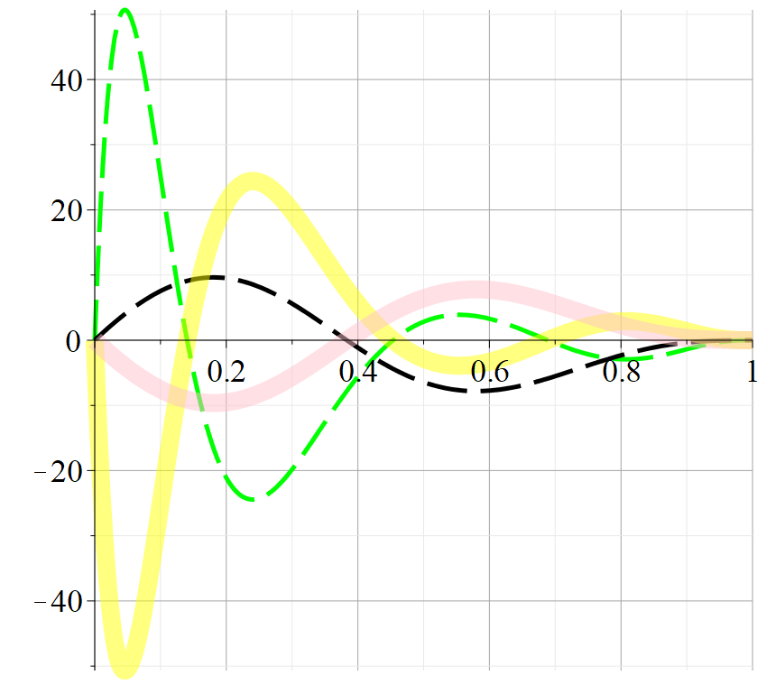
Properties of the approximated polynomials
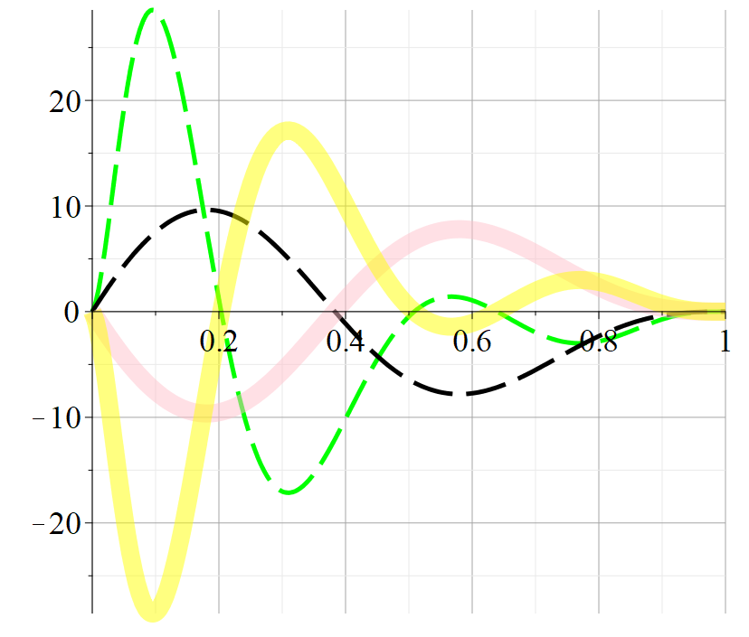
The approximated polynomials were also computed and some of the theoretical results were verified. Indeed, when we investigate the shape properties of the approximated polynomials we notice that they preserve the complementary properties. Of the properties we choose to illustrate here is the behavior of the derivatives. In Figure 3 we plot the derivatives of the approximated polynomials using the variant of the algorithm with input data , and in Figure 4 those obtained with input data We plot the first two derivatives, and observe the following:
- •
;
- •
.
The case of self-dual networks
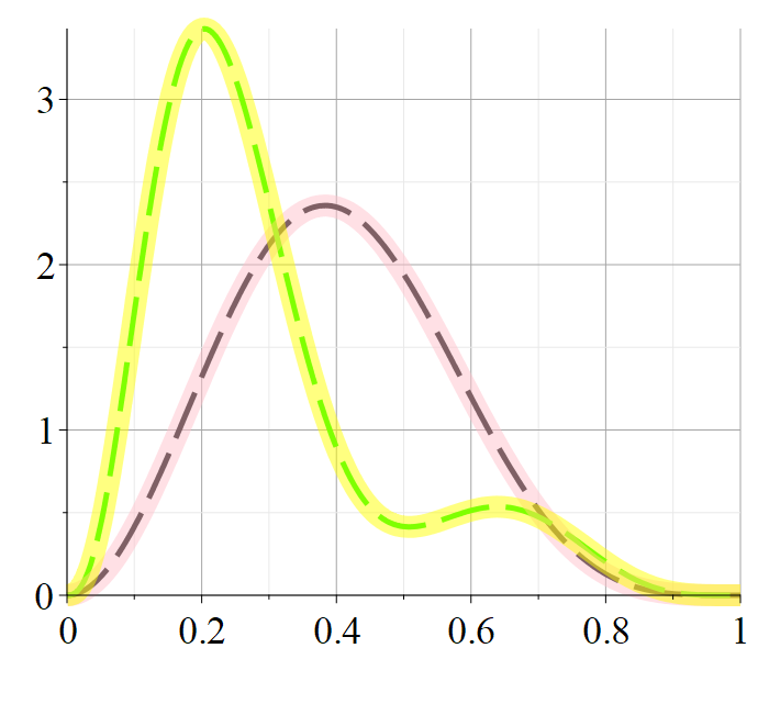
As our method is using some extra information provided by means of duality, we have simulated the case of self-dual networks. We have considered the 5-by-5 hammock network, case for which we have In Figure 5 we have plot the first derivatives of the networks and of the approximations.


Both the reliability polynomial as well as its approximant satisfy This mainly comes from the fact that In this case, the error of approximation is lower than Notice than, even if less information is used for the particular case of self-dual networks, the error of approximation is comparable with the case of smaller networks such as the 3-by-5 hammock. This fact points out that our method could eventually be used in the case of some larger networks.
6 Conclusions
In this paper we have studied the shape properties of the reliability polynomials of two dual networks. Mutual behaviour of these polynomials, referring to high level convexity, inflection points, extremal properties of coefficients functions are studied. The research from [4] and [6] is developed on new bases, taking into account some requirements of shape preserving. We have proposed a technique for simultaneously approximating the reliability polynomials of two dual MMNs, choosing the input data based on their shape properties, in order to obtain results preserving some shapes. Our simulations point out that quadratic splines approach gives much better results than other types of approximation operators, if shape criteria are taken into account together with the size of the error and the complexity of computation. Some possibilities of improving the output are discussed.
Acknowledgments
V.-F. Drăgoi was supported by a grant of the Romanian Ministry of Education and Research, CNCS-UEFISCDI, project number PN-III-P4-ID-PCE-2020-2495, within PNCDI III – ThUNDER2 = Techniques for Unconventional Nano-Designing in the Energy-Reliability Realm.
References
- [1] Jason I. Brown, Charles J. Colbourn, Danielle Cox, Christina Graves, and Lucas Mol. Network reliability: Heading out on the highway. Networks, 77(1):146–160, 2020.
- [2] S. R. Cowell, V. Beiu, L. Dăuş, and P. Poulin. On the exact reliability enhancements of small hammock networks. IEEE Access, 6:25411–25426, April 2018.
- [3] S. R. Cowell, L. Dăuş, V. Beiu, and P. Poulin. On hammock networks - sixty years after. In 2017 12th International Conference on Design Technology of Integrated Systems In Nanoscale Era (DTIS), pages 1–6, April 2017.
- [4] G. Cristescu and V. F. Drăgoi. Cubic spline approximation of the reliability polynomials of two dual hammock networks. Transylvanian Journal of Mathematics and Mechanics, 11(1-2):77–90, December 2019.
- [5] G. Cristescu and L. Lupşa. Non-connected convexities and applications, volume 68. Springer Science & Business Media, 2002.
- [6] Gabriela Cristescu and Vlad-Florin Drăgoi. Efficient approximation of two-terminal networks reliability polynomials using cubic splines. IEEE Transactions on Reliability, 70(3):1193–1203, 2021.
- [7] V. F. Drăgoi and V. Beiu. Studying the binary erasure polarization subchannels using network reliability. IEEE Communications Letters, 24(1):62–66, Jan 2020.
- [8] Vlad-Florin Drăgoi and Valeriu Beiu. Fast reliability ranking of matchstick minimal networks. Networks, n/a(n/a), 2021.
- [9] Vlad-Florin Drăgoi and Gabriela Cristescu. Bhattacharyya parameter of monomial codes for the binary erasure channel: From pointwise to average reliability. Sensors, 21(9), 2021.
- [10] L. Dăuş and Marilena Jianu. Full hermite interpolation of the reliability of a hammock network. Applicable Analysis and Discrete Mathematics, 14:198–220, 2020.
- [11]
L. Dău
and M. Jianu. The shape of the reliability polynomial of a hammock network, Jan 2019. https://ui.adsabs.harvard.edu/abs/2019arXiv190104036D.s , - [12] E. Hopf. Ueber die zusammenhänge zwischen gewissen höheren Differenzenquotienten reeller Funktionen eines Variablen und deren differenzierbarkeitseigenschaften. PhD thesis, Friedrich-Wilhelms Universitat zu Berlin, Berlin, February 1926.
- [13] J. Huh. h-vectors of matroids and logarithmic concavity. Advances in Mathematics, 270:49 – 59, 2015.
- [14] M. Lenz. The f-vector of a representable-matroid complex is log-concave. Advances in Applied Mathematics, 51(5):543 – 545, 2013.
- [15] G. G. Lorentz. Bernstein polynomials. Univ. Toronto Press, 1953.
- [16] E. F. Moore and C. E. Shannon. Reliable circuits using less reliable relays - Part I. Journal of the Franklin Institute, 262(3):191–208, September 1956.
- [17] E. F. Moore and C. E. Shannon. Reliable circuits using less reliable relays - Part II. Journal of the Franklin Institute, 262(4):281–297, October 1956.
- [18] I. P. Natanson. Constructive Function Theory: Vol. I: Uniform Approximation. Frederick Ungar Publishing Company, 1964.
- [19] T. Popoviciu. Sur le prolongement des fonctions convexes d’ordre supérieur. Bull. Math. Soc. Roumaine des Sc., 36:75–108, 1934.
- [20] T. Popoviciu. Sur l’approximation des fonctions convexes d’ordre supérieur. Mathematica (Cluj), 10:49–54, 1935.
- [21] T. Popoviciu. Les fonctions convexes. Actualités scientifiques et industrielles. Hermann, 1945.
- [22] L. Valiant. The complexity of enumeration and reliability problems. SIAM Journal on Computing, 8(3):410–421, July 1979.
- [23] John von Neumann. Probabilistic logics and the synthesis of reliable organisms from unreliable components. Automata Studies, pages 43–98, 1956.
- [24] R. Webster. Convexity. Oxford Univ. Press, 1994.