A Note On Complex Spacetime Metrics
Edward Witten
Institute for Advanced Study
Einstein Drive, Princeton, NJ 08540 USA
For various reasons, it seems necessary to include complex saddle points in the “Euclidean” path integral of General Relativity. But some sort of restriction on the allowed complex saddle points is needed to avoid various unphysical examples. In this article, a speculative proposal is made concerning a possible restriction on the allowed saddle points in the gravitational path integral. The proposal is motivated by recent work of Kontsevich and Segal on complex metrics in quantum field theory, and earlier work of Louko and Sorkin on topology change from a real time point of view.
1 Introduction
In their original paper interpreting black hole entropy in terms of the gravitational action, Gibbons and Hawking [1], after analyzing the thermodynamics of a Schwarzschild black hole, went on to consider black holes with angular momentum. They pointed out that the Kerr metric, assuming that the angular momentum is real, becomes complex-valued when continued to imaginary time. While complex-valued, this metric is everywhere nondegenerate, like all complex metrics that will be considered in this article. Gibbons and Hawking showed that one can recover the expected results for the thermodynamics of the Kerr solution by assuming that this complex saddle point dominates the appropriate path integral.
Somewhat later, Gibbons, Hawking, and Perry [2], observing that the action of Euclidean quantum gravity is not positive-definite, argued that therefore the path integral of “Euclidean” quantum gravity should really be understood as a sort of infinite-dimensional version of a complex contour integral, with the integration running over a suitable family of nondegenerate complex metrics on spacetime.
Since then, other reasons have been put forward to consider complex spacetime metrics and complex saddle points. For example, it has been argued by Halliwell and Hartle [3] that to get sensible answers for the behavior of large, semiclassical spacetimes from the Hartle-Hawking no-boundary proposal for the wavefunction of the universe [4], one must consider complex solutions of Einstein’s equations as saddle points. It has also been argued by Louko and Sorkin [5] that to get sensible answers for real time topology-changing processes, one must consider complex spacetime metrics that correspond roughly to tunneling trajectories. Various additional arguments have been given, some of which will be discussed later.
On the other hand, in considering complex saddle points of Einstein’s equations, one is potentially opening Pandora’s box. Many such saddle points, if included in a functional integral, will give results that are not physically sensible. This point was made in [5], and we will illustrate it further in section 2 with some additional examples. The examples of section 2 are all constructed by taking real submanifolds of simple complex manifolds, so perhaps we should point out that this method of constructing examples is useful but in a sense atypical. There typically is no canonical way to complexify a real manifold or to analytically continue a complex metric , and generically a complex metric on is not related in any useful way to a complexification of .
If some complex metrics are “bad,” which ones are “good”? Consider a semiclassical theory of gravity coupled to matter, and assume that the matter is described by ordinary quantum fields. In that context, an important necessary condition for complex metrics, discussed for example in [3] and [5], is that the complex spacetime should be one in which the quantum field theory of the matter system can be defined. If the matter system is sufficiently generic, the complex spacetime should be one in which more or less any quantum field theory could be defined.
Recently, with a different motivation, Kontsevich and Segal [6] have made a proposal for what is the class of complex geometries in which a generic quantum field theory can be consistently coupled. Their proposal was not directly motivated by quantum gravity; their basic goal was to explore the extent to which traditional axiom sets of quantum field theory can be replaced by the assumption that a theory can be consistently coupled to a certain class of complex metrics. However, it is interesting, though speculative, to consider their class of “allowable” complex metrics in the context of quantum gravity.
In section 3 of this paper, we describe the class of metrics considered in [6] and show that the problematical examples of section 2 are not allowable in their sense. Then in section 4, we consider some of the cases in which apparently useful statements about quantum gravity have been made using complex solutions of Einstein’s equations, and show that the metrics considered are allowable. This gives at least some support for the idea of restricting to “allowable” metrics as saddle points.
In section 5, we discuss from this point of view the integration cycle of the gravitational path integral. As originally discussed by Gibbons, Hawking, and Perry [2], the action of Euclidean quantum gravity is not bounded below. They proposed that the gravitational path integral should be understood as an integral over a real cycle in the space of complex metrics. In the context of perturbation theory around a given classical solution, their proposal is satisfactory, and, if the given solution is allowable, their construction stays in the class of allowable metrics. A satisfactory extension of their proposal beyond perturbation theory is not apparent.
Finally, in Appendix A, we analyze and generalize a question from [5]. The original question involved the Euler characteristic of a two-manifold and the conditions under which it can be computed as , where is the Ricci scalar of a complex metric .
It is a pleasure to submit this article to a volume in honor of the 70th birthday of Frank Wilczek, who was my colleague at Princeton in the 1970’s, and later on the IAS faculty. Frank has made many important contributions to different areas of physics, never shying away from bold speculation. So I hope it is not too inappropriate to submit to this volume a rather speculative article, which is largely motivated by a limited number of examples that are discussed in section 4.11 1 An earlier version of part of this material was presented at a conference in honor of the 70th birthday of another distinguished physicist, Thibault Damour, who also was a colleague of Frank and me at Princeton in the mid-1970’s.
2 Some Examples of Complex Solutions of Einstein’s Equations
The usual flat metric on can be written
| (2.1) |
where is a non-negative real variable and is the usual round metric on a sphere . One simple way to generalize this to a complex invertible metric,22 2 In , this example was briefly described in footnote 5 of [5]. is to leave alone the real sphere but relax the condition for to be real. Instead, we specify that runs over a curve in the complex -plane, for example a curve , where is a real variable. The metric is then
| (2.2) |
This metric is nondegenerate as long as and are both nonzero for all . In that case, the metric is flat. Indeed, if is real, the metric (2.2) just differs from the original flat metric (2.1) by a reparametrization, so it is certainly flat. But when one verifies this flatness, one never has to use the fact that is real, so the metric remains flat even when is complex-valued.
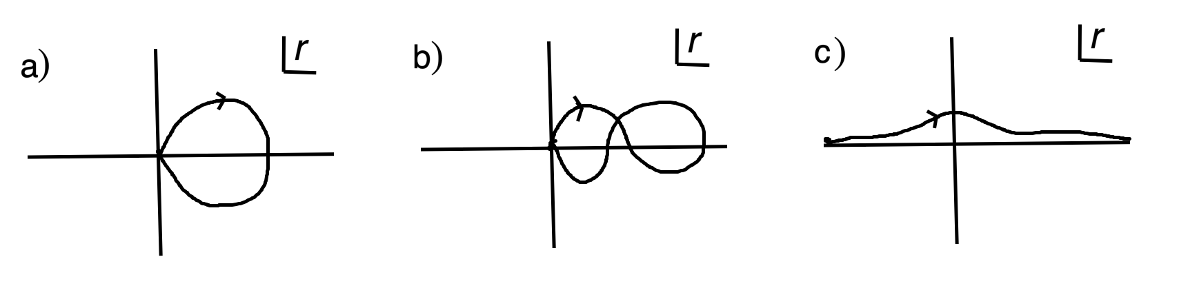
If we want a compact manifold without boundary, we should take to run over a compact interval and require , as in fig. 1(a). Topologically this gives a sphere . The complex metric on that is obtained in this way certainly satisfies the Einstein equations with zero cosmological constant, since it is flat.
We get more options if we complexify the sphere . A unit sphere defined by real variables satisfying can be complexified by simply taking the components of to be complex variables satisfying the same equation. If we complexify as well as the radial variable , we get a complex manifold that comes with a holomorphically varying, complex nondegenerate metric. The metric of a real sphere can be defined as , with the constraint , and, after complexification, the same formula and constraint define a nondegenerate and holomorphically varying complex metric on the complexification of the sphere. So a flat, holomorphic metric on can be written as33 3 As this formula suggests, is closely related to the usual complexification of , which we could have used, albeit less interestingly, in this discussion. It is more convenient to proceed as in the text. . By picking a curve while also keeping the angular variables real, we have described in the last paragraph an embedding of a real -manifold in . Of course, we can consider more general embeddings, or even immersions,44 4 An immersion is a map that is locally an embedding. In the examples described previously, the curve might be immersed rather than embedded in the complex -plane; this will suffice to give a nondegenerate complex metric. of in , with the angular variables no longer real, and this will give more general complex metrics on the same , though the condition that the metric should be everywhere nondegenerate puts a strong constraint on the immersion of in .
What equivalence relation should we place on complex metrics derived from different immersions of a given in the same ? If has been proposed that two complex metrics on obtained by different immersions in the same should be considered equivalent if they differ by “complex diffeomorphisms.” However, it appears difficult to define this notion precisely. It seems that at a minimum, we should insist that two metrics on are equivalent if they come from homotopic immersions of in the same . More optimistically, one might hope that two immersions of in give equivalent metrics if they are merely homologous. Going back to the case that the angular variables are real, in our examples, the first condition would say that two metrics are equivalent if they come from immersed curves and that are homotopic (keeping endpoints fixed) and the second condition would say that for equivalence of the metrics, the curves just have to be homologous. An equivalence relation based on homology is much stronger than one based on homotopy. This is illustrated in fig. 1(b); there are many classes of curves associated to complex flat metrics on that are homologous but not homotopic. (It may be that some of these become homotopic once one allows the angular variables to become complex.)
To get exotic complex flat metrics on , we can simply use the same construction, but now with ranging over the semi-infinite interval . To get topologically, we require ; to get a metric asymptotic to the standard Euclidean metric on , we require for . If we take to be identically equal to for (for some constant ), we get a metric that coincides with the standard Euclidean metric outside a bounded region. Of course, the case just gives back the standard Euclidean metric. We can get other families of complex flat metrics on by choosing the curve to be immersed, rather than embedded, in the complex plane. Provided that approaches sufficiently rapidly at infinity to avoid a boundary term in the Einstein action, all of these flat metrics on have vanishing action, like the standard one.

However, these examples are all equivalent if the appropriate notion of equivalence is based on homology. More interesting are “wormhole” solutions, which we can get if runs over the whole real line. We assume that for and that for all . A simple example is in fig. 1(c). Such a construction gives a connected spacetime (fig. 2(a)) with two “ends” each of which is asymptotic to a copy of ; the ends are connected through a wormhole. So this construction gives complex wormhole solutions of Einstein’s equations with zero action. For additional examples of the same type, we could have at both ends ; the curve could be immersed rather than embedded, and in particular it could wrap any integer number of times around the point .
Given a solution of Einstein’s equations (possibly with matter fields) in which a wormhole connects two different asymptotically flat regions of spacetime, typically one can cut and paste to get an approximate solution in which a similar wormhole connects two distant regions of a spacetime that has only one asymptotically flat end (fig. 2(b)). The ability to do this is based on the fact that far from a wormhole mouth, spacetime is approximately flat. Usually spacetime is only approximately flat far from a wormhole, in which case an exact solution in a world with two asymptotically flat ends leads only to an approximate solution in a world with a single asymptotically flat end. However, in the present context, we can assume that the function in fig. 1(c) is identically equal to for (for some constant ); then the metric in fig. 2(a) is identically equal to the standard Euclidean metric on outside of a compact set on each branch. Given this, the cut and paste procedure required to get a wormhole metric of the sort sketched in fig. 2(b) is exact. So we get complex solutions of Einstein’s equations of wormhole type, with vanishing action, on a spacetime that at infinity reduces to with its standard flat metric.
Finally, we can consider the case that the curve is a circle embedded, or at least immersed, in the -plane minus the point . In this case, we get a flat complex metric on , again with zero action.
Somewhat similarly, we can make exotic complex solutions of Einstein’s equations with a positive cosmological constant starting with the standard metric on a round sphere of radius :
| (2.3) |
One important difference from the flat case is that the action of a compact solution of Einstein’s equation with cosmological constant does not vanish; it is a negative multiple of the volume ,
| (2.4) |
where is the cosmological constant. After solving Einstein’s equations to determine and therefore in terms of Newton’s constant and , one finds that . Thus the action is large and negative if is small and positive, a fact that has been offered as the reason that “the cosmological constant is probably zero” [7]. The de Sitter entropy is defined as .
Rather as before, we can construct complex metrics that solve the Einstein equations with a cosmological constant by considering curves in the complex plane. The resulting metric has the form . First let us discuss compact solutions. The function vanishes at . A curve connecting two of these zeroes, and otherwise avoiding all zeroes, will give a manifold that is topologically . Of course, there are many homotopy classes of such embedded or immersed curves, even after fixing the endpoints. The most basic example is a straight line on the real axis between two consecutive zeroes. This gives the standard real metric on a round sphere. Curves between nonconsecutive zeroes give exotic complex solutions of the Einstein equations. The volume is defined in Riemannian geometry as . In the case of a complex invertible metric, it is not immediately obvious what sign one should take for , and on a manifold that is not simply-connected, in general there can be an inconsistency in defining this sign. For the allowable metrics of Kontsevich and Segal, which we discuss in section 3, there is a natural choice of sign. In the present section, we will not try to be precise about the sign of the volume.
For a metric derived from the round metric (2.3) by a choice of curve , the volume can be computed as the integral of the differential form . (In this formulation, the sign ambiguity appears when one picks an orientation of the cycle on which one wishes to integrate this differential form.) Hence, letting denote the volume of a standard -sphere of unit radius, the volume for a solution based on a curve from to is
| (2.5) |
By Cauchy’s theorem, this integral depends only on the endpoints of the curve, not on the path taken between those endpoints. That happened because the differential form is closed, and means that the volume depends only on the homology class of the curve . For even , vanishes if is even, and equals if is odd. For odd , . Thus, for odd , there exist complex solutions of Einstein’s equations with topology and action much more negative than the action of the standard real solution.
Another basic example is the curve , with . The resulting line element
| (2.6) |
describes de Sitter spacetime of Lorentz signature with radius of curvature . An embedded or immersed curve from to that avoids the zeroes of gives a complex metric that is asymptotic to de Sitter space in the far past and future.
Now suppose that we want a solution of the complex Einstein equations that has no boundary to the past, and coincides with de Sitter space in the future. Such solutions have been discussed in the context of the “no boundary” wavefunction of the universe [4]. We can get such a solution from a curve with running over the half-line , provided is one of the zeroes of , and for large . The case most often discussed is a curve that goes along the real axis from (or ) to and then continues along the imaginary axis from to (or to some given point on the imaginary axis). This is usually described as follows. The path integral along the real axis from to is a Euclidean path integral that prepares an initial state; then the path integral along the imaginary axis up to a point is a Lorentz signature path integral that propagates the state for an arbitrary real time . The Euclidean part of the contour contributes an action (where again is the de Sitter entropy) and the Lorentz signature part of the contour makes an imaginary contribution
| (2.7) |
In a classical approximation, the time-dependent state created by the path integral on this contour is described by the exponential of the action: . The real factor is the norm of the state. The oscillatory factor describes the real time evolution of de Sitter space, as discussed for example in [3].
However, in the world of complex metrics, we can easily construct additional complex metrics that could conceivably represent the creation of de Sitter space from nothing, in the context of the no boundary wavefunction. With still ranging over the half-line , we can choose to be a zero of at , for any , while keeping for large . For odd , this multiplies the real part of the action by and gives a wavefunction proportional to . Thus, naively, we can increase the amplitude to “create a universe from nothing” by increasing .
By taking the curve to be a circle, one can similarly get complex metrics on with zero volume that satisfy Einstein’s equations with a cosmological constant.
What hopefully stands out from this discussion is that many or all of the exotic examples are going to give unphysical results if included in path integrals. One way or another, they must be excluded. With this in mind, after describing in section 3 the allowable metrics of Kontsevich and Segal, we will show that the exotic examples considered in this section are not allowable.
3 Allowable Metrics
On a spacetime of dimension with a complex invertible metric , consider a -form gauge field with -form field strength ; set . The usual action is
| (3.1) |
The metric is allowable, in the sense of Kontsevich and Segal, if has positive real part for every nonzero (real) -form , for any . This amounts to a pointwise condition:55 5 For , this condition was proposed by Louko and Sorkin in footnote 8 of [5] (see also their discussion of eqn. (2.20)). Note that the case suffices in , which is the main case considered in [5]. One might think that one could weaken the condition (3.2) by taking advantage of the fact that obeys a Bianchi identity. This is actually not true, because every -form can be written as a sum , where is a closed -form and is a closed -form ( is the Hodge star). Condition (3.1) for closed and implies (3.2) for arbitrary .
| (3.2) |
for any real, nonzero -form .
A motivation for imposing this positivity is that it makes the path integral of a -form gauge field convergent, for any . The idea in [6] is that quantum field theory in general – not just the free theory of a -form field – is well-defined for a general allowable metric. More specifically, the hope is that this property can substitute for at least some of the standard axioms of quantum field theory. Some evidence in this direction is given in [6]. The condition (3.2) is imposed for all , although the motivation in terms of the field strength of a -form field does not apply for . The condition is just . One way to motivate the case of the condition (3.2) is to observe that a zero-form field is a scalar field, which could have a bare mass . Positivity for real of the real part of the corresponding action gives the case of eqn. (3.2).
Many questions can be asked about whether the condition of allowability is either necessary or sufficient for well-definedness of quantum field theory. We will be rather brief with such questions, as it will not be possible to resolve them definitively. In terms of sufficiency, one can ask whether well-definedness of -form theories for all in a spacetime with a given complex metric is sufficient to ensure well-definedness of general quantum field theories in that spcaetime. Here it is worth noting that free field theories of massless bosonic fields66 6 Bare masses do not help; it is difficult to construct consistent couplings to gravity of massive fields other than -form fields except via Kaluza-Klein theory or string theory [8, 9]. other than -forms do exist, but those theories do not have gauge-invariant stress tensors [10] and therefore cannot be defined in curved spacetime. Moreover, non-free ultraviolet-complete theories of massless fields other than -forms are not known, even in flat spacetime. So -form theories are actually important examples of quantum field theories. For , there are nonlinear versions of -form theories – nonabelian gauge theory for and nonlinear sigma-models for – and for all , there are mildly nonlinear theories in which, for example, the field strength of a -form field is not but , where are forms of degree with . In any of these cases, the real part of the action is positive in an allowable metric. So it is plausible that known quantum field theories that are associated to underlying classical theories can all be consistently coupled to an allowable metric.
Concerning necessity, one might ask if the condition of allowability is unnecessarily strong. For example, let be an allowable metric and let for some real . Replacing by would multiply the action (3.1) by a factor , potentially spoiling the positivity of . Can we compensate by rotating the integration contour for the -form path integral by a phase, ? This might make sense for perturbative fluctuations, but as noted in [6], the partition function of a -form field also involves a sum over quantized integer fluxes that cannot be rotated in the complex plane. So some condition along the lines of allowability is needed, though from this point of view a weaker condition might suffice. Another important point is that one may want the path integral for a quantum field theory in curved spacetime to have a Hilbert space interpretation. For this, the path integral of the matter fields has to be defined by local considerations, not by a completely general analytic continuation. Yet another issue is that the Wick rotation of the matter fields in general may multiply the path integral measure by an ill-defined phase.
In this article, we will not try to address such issues and instead will concentrate on the following two questions. Does a restriction to allowable metrics remove unwanted examples such as the solutions of Einstein’s equations discussed in section 2? And where useful results have come from a consideration of complex solutions of Einstein’s equations, have the metrics in question been allowable? We address the first question here, after summarizing some additional facts from [6], and we explore the second question in section 4.
A simple and useful characterization of allowable metrics was found in [6]. The case of eqn. (3.2) tells us that the real part of the matrix is positive definite. Writing , where and are real, it follows that and can be simultaneously diagonalized by a suitable choice of real basis. (First one picks a basis to put in the form ; such a basis is unique up to an orthogonal transformation, which can be used to also diagonalize .) In such a basis, is diagonal, and therefore so is . Multiplying by the scalar , it follows that is diagonal in this basis:
| (3.3) |
Therefore . Condition (3.2) for tells us to pick the sign of the square root so that . Condition (3.2) now says that for any subset77 7 If is a complex number, then if and only if . Using this, one can see that condition (3.4) for a given set is equivalent to the same condition for the complement of . Hence it suffices to consider sets of cardinality at most . Equivalently, it suffices in this construction to consider -form fields with . This is related to the duality in dimensions between a -form field and a -form field. of the set ,
| (3.4) |
This holds precisely if
| (3.5) |
This statement is Theorem 2.2 in [6].
For example, a Lorentz signature metric is not allowable, since this corresponds to the case . The inequality (3.5) is just barely violated, so a Lorentz signature metric is on the boundary of the space of allowable metrics. In fact, a Lorentz signature metric is on the boundary of the space of allowable metrics in two different ways, since for positive , either of the two metrics
| (3.6) |
is allowable. The difference between the two cases involves the sign of . Since we are instructed in eqn. (3.2) to choose the sign of the square root such that , it follows that for , approaches the positive or negative imaginary axis depending on the sign in eqn. (3.6). Therefore, the sign of the Lorentz signature action (where is the Lagrangian density) depends on the sign of the term. The choice leads to the standard Feynman integral computing real time propagation by , where is the Hamiltonian and appears in the usual Feynman , and the choice leads to a complex conjugate Feynman integral that computes . In the Schwinger-Keldysh approach to thermal physics, one sign leads to propagation of the ket vector and the other sign leads to propagation of the bra. Which is which is a matter of convention. Clearly, the two metrics in eqn. (3.6) cannot be considered “close,” even for small , and one is definitely not allowed to interpolate between them by letting change sign.
Perhaps it is worth stressing that the ability to regularize in this way a Lorentz signature metric as an allowable complex metric does not depend at all on the causal properties of the Lorentz signature metric. So from this point of view, it is perfectly sensible to consider Lorentz signature spacetimes with closed timelike curves.
The criterion (3.5) implies, as was explained in [6], that the space of allowable complex metrics is contractible onto the space of Euclidean metrics.88 8 The space of Euclidean metrics in turn is contractible to a point, by a standard argument. If is some chosen Euclidean signature metric on and is any other such metric, then for , is a Euclidean signature metric. Here we use the fact that the only constraint on a real symmetric tensor to make it a Euclidean signature metric is that it should be positive-definite; if and have this property, then so does . By letting vary from 0 to 1, we contract the space of all Euclidean signature metrics on onto the metric , showing that the space of Euclidean signature metrics is contractible. Note that this argument is not valid (and the conclusion is not true) for real metrics of Lorentz signature, or any signature other than Euclidean signature. Indeed, eqn. (3.5) implies that for all , is not on the negative real axis, so there is a canonical path to rotate to the positive real axis while always satisfying the condition (3.5): one rotates in the upper half plane if , and in the lower half plane if . It follows that any topological invariant that can be defined using an invertible metric, such as the integrals that define the Euler characteristic or the Pontryagin numbers of , takes the same value for an allowable complex metric as for a Euclidean metric. It was shown in [5], with the example of the Gauss-Bonnet integral in two dimensions, that in general this is not true for complex invertible metrics. We return to this point in Appendix A.
The case of eqn. (3.2) implies that if is a manifold with allowable metric, then its volume has positive real part. In [6], it is shown that eqn. (3.5) implies that if has an allowable complex metric, then the induced metric on any submanifold of is also allowable. Hence the volume of any such has positive real part. One can take this as an indication that perturbative strings and branes make sense on a manifold with allowable complex metric. (In the case of perturbative string theory, one will need to impose worldsheet conformal invariance, as in the more familiar case of a Euclidean metric on .)
Now we will use eqn. (3.5) to show that the problematic examples of section 2 are not allowable,. First consider the flat metrics of the form , where is a curve in the complex plane. If there is any value of for which is imaginary, then at that value of , is negative-definite, so of the in eqn. (3.3) are negative and eqn. (3.5) is not satisfied at that value of . If is never imaginary, then (except for possible endpoints at ) the curve is contained in one of the half-planes and . If the curve is homotopic to the positive or negative axis, the corresponding metric is equivalent to the standard flat metric on . Otherwise, there is some value of at which has a maximum or a minimum. At such a point, so is imaginary. Hence is negative definite and one of the in eqn. (3.3) is negative, contradicting eqn. (3.5). The behavior near a maximum or minimum of actually consists of a forbidden transition between the two choices of sign in eqn. (3.6).
Finally, consider the metrics that satisfy Einstein’s equations with a cosmological constant. Here is a curve that avoids the points , , except at endpoints. For an allowable metric, must be nonzero, except possibly at endpoints; otherwise is negative definite and eqn. (3.5) is violated. To avoid vanishing of , the curve must be confined to a strip , for some . This excludes many of the exotic possibilities described in section 2, including the closed universes and the solutions describing “creation of a universe from nothing” that have action more negative than the standard values. The other exotic possibilities are excluded by the fact that cannot have a maximum or minimum along the curve, since at such a maximum or minimum, is negative definite.
4 Some Useful Complex Saddles
Our goal in this section is to examine some examples in which results that appear to be physically sensible have been obtained by considering complex metrics on spacetime. We will see in these examples that the metrics in question are allowable. However, we consider only a few examples and it is not clear what conclusions can be drawn.99 9 There are also proposals in the literature for applications of some non-allowable metrics. See for example [11].
4.1 Topology Change In Lorentz Signature
The first example that we will consider is topology change in Lorentz signature, which was considered originally by Louko and Sorkin [5] from a similar point of view. See for example [12, 13, 14, 15] for further discussion of topology change in real time.
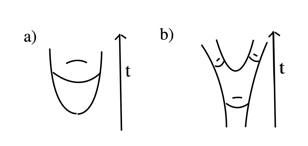
For closed universes in two spacetime dimensions, the basic examples of topology change are the creation of a closed universe from nothing (fig. 3(a)), the splitting of a closed universe in two (fig. 3(b)), and the time reverses of these. Neither is possible with a smooth and everywhere nondegenerate Lorentz signature metric. However, it is possible to pick a Lorentz signature metric which is smooth, and is nondegenerate except at one point in spacetime, at which the topology change occurs. For example, on a spacetime that describes creation of a closed universe from nothing, we can take real coordinates such that the creation event occurs at , and consider the line element
| (4.1) |
with a constant . The metric (4.1) smooth, and is nondegenerate except at . At , the metric is degenerate – it vanishes. Provided that , this metric has Lorentz signature except at ; can be viewed as a “time” coordinate, and the metric describes a circle that is “created” at and grows in proportion to .
Some regularization is required, since presumably the coupling of quantum fields to a degenerate metric is not well-defined. One way to regularize the metric is to replace the line element with1010 10 Louko and Sorkin used a slightly different regulator that is also consistent with eqn. (3.5) in a suitable range of .
| (4.2) |
In the framework discussed in the present paper, should be nonzero for all because a Lorentz signature metric is regarded as a limiting case of a complex invertible metric that satisfies eqn. (3.5). The role of is to make the metric nondegenerate for all ; for this, should be positive at but can vanish except very near that point. To see that the line element (4.2) corresponds to an allowable metric, let be the one-form , and let be a one-form that is orthogonal to . Then for , (4.2) has the general form
| (4.3) |
This is manifestly consistent with eqn. (3.5). At , the metric has Euclidean signature and again eqn. (3.5) is satisfied.
Splitting of a closed universe into two can be treated similarly. One can pick a “time” coordinate whose differential is nonzero except at an isolated saddle point, at which the topology change occurs (fig. 3(b)). Near the saddle point, one can pick local coordinates with . The line element , describes a smooth metric that has Lorentz signature everywhere except at the saddle point, where it vanishes. This again can be regularized to give an allowable complex metric .
Now consider the case that spacetime is a closed two-manifold of genus . The Gauss-Bonnet integral appears in the action of “Euclidean” quantum gravity with a negative coefficient. If we pick on a Euclidean signature metric , then the Gauss-Bonnet theorem gives . On the other hand, it is possible to pick on a Morse function which has one local minimum, one local maximum, and saddle points (fig. 4). Together these points are called the critical points of . As noted by Louko and Sorkin [5], given and , one can construct the metric
| (4.4) |
which is everywhere smooth, and has Lorentz signature except at the critical points, where it vanishes. A simple regularization that gives an allowable complex metric is to replace with
| (4.5) |
with near critical points (but potentially vanishing except near critical points) and . Now let us consider the Gauss-Bonnet integral for this kind of metric. As noted by Louko and Sorkin, is imaginary for a Lorentz signature metric, and therefore in the limit , the expected real contribution from must be localized at the critical points of the function . Indeed, they showed that a local maximum or minimum of contributes to , while a critical point contributes . As was explained in section 3, the Gauss-Bonnet integral has its standard value for an allowable complex metric. This is not so for a general complex metric, as observed by Louko and Sorkin and further discussed in Appendix A.

Topology change in Lorentz signature in any dimension can be treated similarly. On any manifold , one can choose a “Morse function” that has only isolated, nondegenerate critical points. A metric of the form (4.5) is smooth and has Lorentz signature except at the critical points, where it vanishes. The regularization (4.5) makes sense in any dimension and gives a complex allowable metric.
4.2 The Hartle-Hawking Wavefunction
An important application of complex spacetime metrics is to the Hartle-Hawking wavefunction of the universe [4]. In dimensions, one considers a -dimensional manifold with metric . The Hartle-Hawking wavefunction is formally defined by a sum over all manifolds with boundary , with the contribution of each to the sum being the gravitational path integral over metrics on that restrict on the boundary to .
A saddle point in this context is a classical solution of the Einstein equations on that restricts to on . This problem makes sense for Euclidean metrics. If the Einstein-Hilbert action in Euclidean signature were bounded below, one might hope that real saddle points would exist – a metric that minimizes the action for given would be an example. Such a real saddle point might fail to exist if when we try to minimize the action, develops a singularity. The analog of this actually happens for instantons in Yang-Mills theory with Higgs fields on ; in an instanton sector, there is no true classical solution, since the action can be reduced by letting the instanton shrink to a point. Similar behavior can occur in gravity; see for example [16]. Even if a classical minimizer does not exist, if the action were bounded below, it would have a greatest lower bound and the asymptotic behavior of the Hartle-Hawking wavefunction, near a classical limit or when describes a manifold of large volume, would be . If the greatest lower bound on the Euclidean classical action is not achieved by any smooth classical field (because a singularity develops when one tries to minimize the action), but can be approximated by a sequence of smooth classical fields, one could describe this roughly by saying that there is no true saddle point but there is a virtual saddle point at infinity in field space, analogous to a point instanton in Yang-Mills theory.

In many known examples, the gravitational path integral in the semiclassical limit is dominated by a critical point at infinity rather than a conventional critical point; for one such example, see fig. 5. In all cases in which any candidate has been suggested for the semiclassical behavior of a gravitational path integral, it is dominated by a conventional critical point or a critical point at infinity. The reason for this is just that if a critical point, possibly at infinity, has not been found, then the asymptotic behavior of the gravitational path integral is unknown. From the standpoint of a possible ultraviolet completion of Einstein gravity, there is potentially no fundamental difference between an ordinary critical point and a critical point at infinity. What looks in one description like a singular configuration might be perfectly smooth in a more complete description. Precisely this has happened to many types of singularity in gauge theory and gravity that have turned out to be perfectly smooth from the vantage point of string theory. In Morse theory, where topological meaning is given to the critical points of a function, it is a standard fact that on a non-compact manifold in general one has to include critical points at infinity. So their appearance in the gravitational path integral, where one deals with critical points of the action functional on the noncompact space of all real or complex metrics on a manifold , should not be too much of a surprise.
In fact, however, the Euclidean action for gravity is unbounded below, and in general the boundary value problem associated to the Hartle-Hawking wavefunction is believed to have no classical solution of Euclidean signature (not even a virtual solution at infinity). For instance, consider Einstein’s equations with positive cosmological constant and choose to be a sphere with a round metric with a very large radius of curvature (compared to the length scale set by ). It is believed there is no real classical solution, not even in a limiting sense.
As is explained in [3], this phenomenon is actually a necessary condition for the Hartle-Hawking wavefunction of the universe to make sense in the context of cosmology. If the Einstein-Hilbert action in Euclidean signature were positive-definite like the action of a conventional scalar field, then the wavefunction would behave semiclassically as , as noted earlier, where is the greatest lower bound on the action. If gravity had similar positivity properties to scalar field theory, where the action is strictly positive unless the field is constant, we would expect to be strictly positive except in very special cases. By a simple scaling argument, would grow if the metric on is scaled up to large volume, and hence the Hartle-Hawking wavefunction would vanish exponentially when is large. This exponential decay of the wavefunction for large volumes would be analogous to the fact that, for a real scalar field , a wavefunction defined similarly to the Hartle-Hawking wavefunction vanishes exponentially for large . The scalar analog of the Hartle-Hawking wavefunction is defined by choosing a particular with boundary , and performing a path integral over fields on that restrict to on . This wavefunction vanishes exponentially for large because the usual action of a scalar field is positive-definite, and grows when the boundary values are increased. In fact, the action grows quadratically with so the wavefunction vanishes as the exponential of .
In the case of gravity, the Hartle-Hawking wavefunction can behave differently because, as the Euclidean action is not bounded below, it is possible for there to be no real critical point (even at infinity), and the integral can potentially be dominated by complex critical points. For instance, in the example of the round sphere of large radius in a world with , though there is no real saddle point, there are complex saddle points that give an oscillatory contribution to the path integral. Moreover, this contribution can be large near a classical limit, because the real part of the “Euclidean” action can be negative. As explained in the discussion of eqn. (2.3), there are both conventional complex saddles, which involve trajectories from to a point on the imaginary axis, and unconventional ones, which start at , . The unconventional ones lead to apparently unphysical behavior, but we noted at the end of section 3 that they are not allowable. An equally important fact is that the conventional saddle points, starting at , are allowable. To get an allowable metric, we can start with the usual idea of a straight line from to joined to a straight line from to , and modify this slightly to get a smooth path along which is everywhere nonzero. This gives the allowable metric .
As many authors have pointed out, although the exponentially large amplitude for this allowable trajectory that “creates a universe from nothing” is interesting, it cannot be the whole story for cosmology, since this mechanism would tend to produce an empty universe with the smallest possible positive value of the cosmological constant. For an alternative treatment of these solutions, based on a different boundary condition in which the second fundamental form of the boundary is fixed, rather than the metric of the boundary, see [17].
4.3 Timefolds
In many contexts, for instance in real time thermal physics and in various analyses of gravitational entropy, such as [18, 19, 20], it is convenient to consider path integrals that in a sense zigzag back and forth in time. For example, given an initial state and an operator , one might want to calculate . To describe this as a path integral, we need a path integral that propagates the state forwards in time by a time to construct the factor , after which we insert the operator and then apply a path integral that will propagate the state backwards in time to construct the factor .
As explained in section 3, from the point of view of allowable complex metrics, the two cases of forwards and backwards propagation in time correspond to two possible regularizations of a Lorentz signature metric, in which, for example, is replaced by .
Thus, if we do not mind working with a discontinuous metric, we can describe the timefold with the discontinuous metric
| (4.6) |
with
| (4.7) |
However, to couple quantum fields to a discontinuous metric is likely to be problematical. To get something better behaved, we should replace with a smooth function that equals for (say) , for some small , and for . The only subtlety is that is not allowed to pass through the positive real axis, as this would violate the condition (3.5) for an allowable metric. So has to go “the long way around” from in the lower half plane through the negative real axis and finally to in the upper half plane (fig. 6). The portion of this path in which gives some imaginary time propagation that regularizes the real time path integral that we would naively compute using the real but discontinuous function in eqn. (4.7).

4.4 The Double Cone
Somewhat similar to a timefold is the double cone, which has been used [21] to study the spectral form factor in a holographic theory. A simple version of the double cone metric in two dimensions is
| (4.8) |
If is a real variable with an identification , and is real and nonnegative, then this metric describes a cone, with Lorentz signature and with a singularity at (where one identifies points with different values of ). However, in the application to , one wishes to allow negative as well as positive values of . In this case, still identifying , one has a pair of cones, meeting at their common apex. In a holographic interpretation, the conformal boundaries of the two cones are related to the two traces in the spectral form factor.
This rather singular spacetime has a rather simple regularization, essentially discussed in [21], in which we avoid letting pass through the origin in the complex plane. We simply take, for example,
| (4.9) |
leading to the metric
| (4.10) |
Here is a small nonzero real number, whose sign is not important, in the sense that one can compensate for changing the sign of by , . As will be clear in a moment, this would have the effect of reversing which of the two cones computes in a holographic context and which computes .
The function is never positive for real , so is never negative, and therefore the line element in eqn. (4.10) corresponds to an allowable complex metric. For positive , is close to the positive imaginary axis, and for negative , it is close to the negative imaginary axis. Accordingly, with standard conventions, the positive cone is related in a holographic description to , and the negative cone is related to .
Also analyzed in [21] is a regularized version of the double cone that is related to . The line element is
| (4.11) |
Again this is an allowable complex metric.
4.5 Rotating Black Holes
The last example that we will consider is a rotating black hole.
Gibbons and Hawking [1] computed the thermodynamic properties of a Schwarzschild black hole by computing the action of a smooth Euclidean signature solution of Einstein’s equations obtained by continuing the Schwarzschild solution to imaginary time. They then considered a rotating or Kerr black hole, and observed that in this case continuation to imaginary time gives a complex metric,1111 11 This statement assumes that one continues to imaginary time while keeping the angular momentum real. If one also takes the angular momentum to be imaginary, then there is a real solution in Euclidean signature. One approach to black hole thermodynamics is to compute for imaginary angular momentum using a real Euclidean metric and then continue back to real angular momentum. This seems to give sensible results. However, it is natural to ask what happens if we keep the angular momentum real. The physical meaning of the imaginary angular momentum “ensemble” based on is not very transparent. We put the word “ensemble” in quotes because the operator is not positive, so in taking its trace, we are not counting states with positive weights. It is not clear what states dominate this trace, or even whether this question has a clear answer. which they called quasi-Euclidean. It turned out that the thermodynamic properties of a Kerr black hole can be computed from the action of the quasi-Euclidean solution, with physically sensible results that are in accord with other approaches.
From the perspective of the present article, it is natural to ask if the quasi-Euclidean metric is an allowable complex metric. In general, the answer to this question is “no.” For example, let us consider the case of a black hole in an asymptotically flat spacetime. In the field of a stationary, rotating black hole, a quantum field has at least two conserved quantities – the energy and angular momentum . (Above dimensions, there might be more than one conserved angular momentum component.) The partition function of a quantum field propagating in the black hole spacetime is a contribution to , where and are the inverse temperature and the angular velocity of the black hole. In the case of a black hole in asymptotically flat spacetime, a particle of given energy can have arbitrarily large if it is located far from the black hole. Hence such a particle can make an arbitrarily large contribution to , and one should not expect to get a sensible answer for a quantum contribution to . Hence it is natural that the coupling of quantum fields to the quasi-Euclidean metric would be ill-defined, and that this metric would not be allowable.
In Minkowski space, for example, if corresponds to the rotation generator , then corresponds to the vector field
| (4.12) |
This vector field is spacelike for , and hence a particle localized at can have an arbitrarily negative value of . The same is true in an asymptotically flat Kerr spacetime.
It was observed in the early days of the AdS/CFT correspondence that matters are better in an asymptotically Anti de Sitter (AAdS) spacetime [22, 23, 24]. In conformal field theory on a unit sphere, the operator is bounded below if , and the trace converges under that restriction on . Therefore, in the bulk dual to a boundary conformal field theory, one expects the partition function to make sense for small enough.
In AAdS space, pick a rotating black hole solution with the property that outside the black hole horizon, the Killing vector field that corresponds to is everywhere timelike. One expects that to be the condition that makes the quantum operator bounded below for perturbations outside the horizon, ensuring that the trace , taken over quantum fluctuations outside the horizon, is well-defined. The path integral on the quasi-Euclidean metric is supposed to be a way to compute that trace. So under these conditions, we may hope that the quasi-Euclidean metric might be allowable. In fact, as we will explain, the quasi-Euclidean metric is allowable if and only if the vector field is everywhere timelike outside the horizon.
In four dimensions, a rotating black hole is conveniently parametrized by coordinates , where and are generated by and , respectively ( is an angular variable with ), and in the asymptotic region, is a radial coordinate and are polar angles. In three dimensions, one can omit from this discussion; above four dimensions, some additional coordinates are needed but the essence of the following argument is not changed, as we will explain at the end. A general form of the metric of a rotating black hole is
| (4.13) |
All functions and depend on only. This form is partly constrained by the fact that a rotating black hole has a symmetry under . We have assumed a coordinate choice such that , though this will not be important. The function vanishes at ; this is part of the AAdS condition. On the horizon, has a constant value ; this fact is important in constructing the quasi-Euclidean spacetime. Indeed, the constant is the quantity that appears in the black hole thermodynamics. It is convenient in constructing the quasi-Euclidean spacetime to define a new angular coordinate . The line element is then
| (4.14) |
In this coordinate system, the vector field that generates is just . The condition for to be everywhere timelike outside the horizon is therefore simply or
| (4.15) |
This function vanishes on the black hole horizon, where becomes null.
In the coordinate system , the quasi-Euclidean metric is constructed by discarding the region behind the horizon, setting , and identifying points on the horizon that differ only in the value of . The quasi-Euclidean metric is thus
| (4.16) |
In showing that this is smooth, one uses the vanishing of on the horizon.
It is rather immediate from the definitions that a metric of this form is allowable if and only if, treating and as constants, the purely two-dimensional metric that corresponds to the line element
| (4.17) |
is allowable. This condition is trivial on the horizon, where is Euclidean. Away from the horizon, we have a line element of the general form
| (4.18) |
with real . Such a metric is allowable if and only if . To see necessity, observe that such a metric has , so the necessary condition for allowability reduces to , that is, . Sufficiency of can be seen by observing that for , can be put in the form (3.3) with .
The condition is equivalent to eqn. (4.15), and it is also true that outside the horizon, since the black hole metric would fail to have Lorentz signature if is not positive outside the horizon. Thus we have shown that the quasi-Euclidean metric is allowable if and only if the vector field that generates is everywhere timelike outside the horizon.
Above four dimensions, rotating black holes are more complicated [25]. However, the complications do not really affect the preceding analysis. Consider a black hole solution that has a Killing vector field that is everywhere timelike outside the horizon, and pick coordinates so that this Killing vector field is just ; denote the other coordinates as . The metric then has the general form
| (4.19) |
where , , and depend only on . The function vanishes on the horizon and is negative outside, and is positive-definite outside the horizon. The quasi-Euclidean solution is obtained as before by substituting , omitting the region behind the horizon, and identifying points on the horizon that differ only in the value of . Alowability is a pointwise criterion, and in checking this criterion at a given point, only one linear combination of the is relevant, namely . Therefore, allowability of the quasi-Euclidean metric again comes down to the fact that a two-dimensional metric of the form (4.18) is allowable for .
A simple example of a rotating black hole with a Killing vector field that is everywhere timelike outside the horizon is the BTZ black hole in three dimensions. Consider a BTZ black hole of mass and angular momentum in a world of radius of curvature . Black hole solutions exist for , with
| (4.20) | ||||
| (4.21) | ||||
| (4.22) | ||||
| (4.23) |
The horizon is at , so . A short calculation reveals that
| (4.24) |
which is positive outside the horizon, that is for .
5 Searching for the Integration Cycle of the Gravitational Path Integral
In [2], Gibbons, Hawking, and Perry (GHP) observed that the Einstein action in Euclidean signature is unbounded below. In fact, if one makes a Weyl transformation of the metric by , the action picks up a negative term proportional to . To deal with this, GHP proposed to Wick rotate the integration contour for the scale factor of the metric tensor, setting with real. They considered the path integral for asymptotically flat metrics on a space that is asymptotic to at infinity, and argued that every such metric can be uniquely written1212 12 In situations other than asymptotically flat metrics on , one needs to somewhat modify the GHP proposal. Some issues concerning this proposal were discussed in [3]. as , where is a metric of zero scalar curvature. GHP formulated a “positive action conjecture,” according to which the Einstein action is nonnegative for an asymptotically flat metric of zero scalar curvature. The combination of the positive action conjecture for and the contour rotation for was supposed to make the gravitational path integral convergent. The positive action conjecture was later proved by Schoen and Yau [26].
At least in the context of perturbation theory around a classical solution, the GHP procedure does make sense of the gravitational path integral, modulo the usual problems concerning ultraviolet divergences. In the Gaussian approximation, setting , with real , makes the action positive and the path integral convergent. In perturbation theory, one is always integrating the product of a polynomial times a Gaussian function, and, provided that the Gaussian is convergent, such an integral is well-defined. So there are no further difficulties in perturbation theory, except for the usual ultraviolet divergences of quantum gravity.
Should one do better? One possible point of view is that the gravitational path integral only makes sense in perturbation theory around a classical solution, and to do better requires a better theory. However, it is also imaginable that extending the GHP recipe to make sense beyond perturbation theory would be a step towards a better theory. To go beyond perturbation theory, one would want an integration cycle in the space of complex-valued metrics such that the real part of the Einstein action grows at infinity along – ensuring at least formally that the gravitational path integral converges as an integral on . Extrapolating from [2], an obvious guess might be to define by saying where is an angle-valued field and is a real metric of zero scalar curvature. This is not satisfactory because with this choice, the gravitational action has no useful positivity property; it changes by an arbitrary phase when is shifted by a constant.
From the perspective of the present paper, one would like to be contained within the space of allowable complex metrics. One can attempt to use gradient flow to construct the integration cycle , as described in detail for three-dimensional Chern-Simons theory in [27]. In perturbation theory, this procedure will be equivalent to that of [2], but it might extend beyond perturbation theory. The general procedure is as follows. Let , be a set of fields or integration variables, with an action , so that the integral of interest is formally . The goal is to generalize this integral, which may not converge, to a convergent complex contour integral. As a first step, analytically continue the to complex variables , and analytically continue the action to a holomorphic function . The are functions on a space and the are holomorphic functions on a complexification of . The goal is now to find a middle-dimensional integration cycle , such that the integral , which formally reduces to the original if , converges.
This may formally be done as follows.1313 13 See [28] for a discussion of this formalism in the context of gravity (and an introduction to the formalism). The perspective taken there is that the Lorentz signature path integral is the basic definition, and analytic continuation to complex metrics is used only as a procedure to more precisely define and evaluate it and deal with any ambiguities. A consequence is that complex critical points can only make exponentially small contributions, not exponentially large ones. So in particular the enhancement in the “creation of a universe from nothing,” discussed in section 4.2, is replaced by an suppression. Pick a positive-definite metric on . In the previously mentioned application of this formalism to Chern-Simons theory, a simple choice of leads to a relation with renormalizable gauge theory in four dimensions. In gravity, since we are dealing anyway with a highly nonlinear low energy effective field theory, we can contemplate a rather general choice of . We will, however, assume that is a Kahler metric , as this leads to some simplifications. Introduce a “flow variable,” a real variable , and view the as functions of . Now consider the gradient flow equation
| (5.1) |
In an application to -dimensional field theory on a -manifold , this equation is really a differential equation on a -manifold , where is parametrized by . The solutions of the gradient flow equation in which is independent of correspond to critical points of the action function or in other words to classical solutions of the equations of motion. In any nonconstant solution, is a strictly increasing function of .
Let be a critical point of the action,1414 14 In all of the following statements, one has to allow critical points at infinity as well as ordinary critical points. Critical points at infinity were discussed in section 4.2. which for simplicity we will assume to be isolated and nondegenerate. (The discussion can be generalized to include other cases.) Because the function is the real part of a holomorphic function, the matrix of second derivatives of at , which is known as the Hessian matrix, has equally many positive and negative eigenvalues.1515 15 For example, if has complex dimension 1, we can pick a local holomorphic coordinate on near a critical point so that . Then , and clearly the Hessian matrix of this function has one positive and one negative eigenvalue. Now consider solutions of the gradient flow equation on a semi-infinite interval that start at at . Because half the eigenvalues of the Hessian at are positive and half are negative, the values of such a solution at comprise a middle-dimensional submanifold . In a finite-dimensional context, under mild assumptions,1616 16 The main assumption needed is that there is no solution of the flow equation on the whole real line that flows from one critical point at to another one at . A sufficient condition to ensure that no such flow exists is that the different critical points have different values of . This statement depends on the metric being Kahler. If there is a flow between two distinct critical points and , one says that one is sitting on a Stokes line (in the space of all possible actions ), and the statements in the text require some modification. the function grows at infinity along and the integral converges. Moreover, again under some mild assumptions, any integration cycle such that the integral converges is an integer linear combination of the .
In gravity, would be the space of all metrics on a manifold and is the space of complex-valued metrics on . The diffeomorphism group of acts on , and the path integral is really an integral over . Upon complexification, is replaced by . One might naively think that would have a complexification and that one would really want to define a cycle in . This is wrong for two reasons. First, although the Lie algebra of can be complexified to a complex Lie algebra , there is no corresponding complexification of the group , so there is no way to define a quotient . Second, even in gauge theory, where a complexification of the gauge group does exist, the gradient flow equation is not invariant under this complexification. The appropriate procedure to deal with gauge symmetries was described in [27]. One replaces the action with an extended action , where is a Lagrange multiplier and is a moment map for the imaginary part of . Roughly, is a partial gauge-fixing condition that reduces invariance under to invariance under . Then one proceeds as before, studying the flow equation of this extended action.
Unfortunately, it seems doubtful that this procedure will really accomplish what we want in the case of gravity. With a simple choice of the metric , there is no obvious reason for to remain in the space of allowable metrics. We could choose to be a complete Kahler metric on the space of allowable metrics. This will force to remain in the space of allowable metrics, but the real part of the action might not go to along .
An alternative to this discussion – and to the framework of the present article – would be to use gradient descent to define an integration cycle not for gravity alone but for the combined system of gravity plus matter fields. One would simply follow the above-described procedure, but taking to be the combined action of gravity plus matter. In this case, all critical points are potentially allowed; one simply Wick rotates all gravitational or matter field variables to make any integral converge. Another mechanism has to be found to exclude undesirable examples such as those of section 2. As remarked in section 3, the sum over discrete fluxes for matter fields may be a problem in such an approach, and one also would have to accept that in expanding around a critical point, the matter path integral does not have a Hilbert space interpretation. The reason for the last statement is for a path integral on a manifold to have a Hilbert space interpretation, the field variables and integration cycle have to be defined by local conditions on ; an integration cycle produced by gradient descent (or in perturbation theory by Wick rotating any mode whose kinetic energy has a real part with the wrong sign) does not have the appropriate locality. Still another issue is that Wick rotating the matter fields multiplies the path integral measure by a potentially ill-defined phase.
One last comment concerns the positive action theorem. Consider instanton solutions of Einstein’s equations with zero cosmological constant that are asymptotic to at spatial infinity. It is not difficult to prove that such a solution has zero action.1717 17 The bulk term in the action vanishes for a Ricci flat metric, and the linearized Einstein’s equations imply that a solution that is asymptotic to flat at spatial infinity approaches the flat metric on fast enough that the Gibbons-Hawking-York surface term in the action also vanishes. It would presumably not be physically sensible to include in the gravitational path integral an instanton with zero action, since its contribution to the path integral would be too large, so one is led to hope that such solutions do not exist. Indeed, a special case of the positive action conjecture of [2], proved in [26], says that the Einstein equations in Euclidean signature with zero cosmological constant have no solution asymptotic to other than itself. With complex metrics, this is not so, as we saw in an example in section 2. Optimistically, an extension of the positive action theorem might say that the real part of the action is always positive for an allowable classical solution that is asymptotic to at infinity. Alternatively, perhaps allowability is not the right condition or not a sufficient condition.
Acknowledgments I thank R. Bousso, J.-L. Lehners, L. Iliesiu, J. Maldacena, S. Murthy, H. Reall, G. Segal, S. Shenker, R. Sorkin, M. Taylor, and J. Turiaci for helpful discussions. Research supported in part by NSF Grant PHY-1911298.
Appendix A Pontryagin Classes, Euler Classes, and Volumes
Here we discuss topological aspects of the strange world of nondegenerate but possibly nonallowable complex metrics.
The Chern classes of a rank complex vector bundle over a manifold can be described in de Rham cohomology by familiar expressions involving the curvature of any connection on . For example, the second Chern class is associated to the four-form . Depending on the dimension of , Chern numbers of can be defined as integrals over of products of Chern classes.
This construction is probably most familiar in the case that the structure group of is , but it is valid more generally if is a connection with structure group .
If instead is a rank real vector bundle over , then its Pontryagin classes are defined as the Chern classes of the complexification of . The Pontryagin classes of a manifold are defined as the Pontryagin classes of its tangent bundle . So in other words, they are by definition the Chern classes of the complexification of , and they can be computed using any connection, in general of structure group , on . So given any connection on with curvature , the Pontryagin classes of can be defined by the usual polynomials in .
In particular, suppose we are given a nondegenerate complex metric on , not necessarily allowable. The standard formulas defining the Levi-Civita connection on the tangent bundle of make sense in this situation, but if is not real, they give a complex-valued connection. In other words, the Levi-Civita connection associated to a complex metric is a connection on . The structure group of this connection is in general , a subgroup of . But as we have just noted, Pontryagin classes can be defined using the curvature of any connection on . So in particular, Pontryagin numbers of can be computed using the Riemann curvature tensor of any complex-valued metric. For example, if is a four-manifold, the integral associated to the first Pontryagin class will always have its standard value.
One way to understand this statement is the following. If is a non-allowable complex metric on , it may not be possible to interpolate continuously in the space of invertible complex metrics between and a Euclidean metric . But it is always possible to continuously interpolate between the Levi-Civita connection derived from and the Levi-Civita connection derived from : one just considers the family of connections on defined by , . (The interpolating connections in general have structure group .) So they give the same results for Pontryagin classes.
In dimension , another interesting curvature integral is the integral that appears in the Gauss-Bonnet formula for the Euler characteristic of . As was noted by Louko and Sorkin1818 18 They illustrated the point with a nondegenerate complex metric on whose curvature vanishes, so the usual Gauss-Bonnet integral gives the value 0, not the standard Euler characteristic 2 of . Their example of the complex flat metric on was described in section 2. [5] in the case , it is not true that in general the Gauss-Bonnet integral computed using the curvature of a nondegenerate complex metric takes its standard value. In the case of the curvature formula for the Euler characteristic, the underlying invariant is the Euler class of an oriented real vector bundle. The differential form that represents the Euler class of a real vector bundle is a multiple of , where we view as a two-form valued in antisymmetric matrices (generators of the Lie algebra of ). Thus the definition uses the fact that there is a symmetric order invariant on the Lie algebra of , namely the tensor (in a different language, the invariant is the Pfaffian of an antisymmetric matrix). There is no such invariant on the Lie algebra of (or even ). But there is such an invariant in . So without more structure, a rank complex vector bundle does not have an Euler class. However, if we are are given a reduction of the structure group of to , then one can define a Euler class of . It is not a topological invariant of but depends on the topological choice of the reduction of structure group to .
Applying this to complex metrics on , we observe that a complex nondegenerate metric determines a reduction of the structure group of to . If the structure group can be further reduced to (which is the case if the Levi-Civita connection derived from has holonomy in ), then this enables one to define an Euler class of . This Euler class can be represented by the standard curvature polynomial. However, the Euler class of defined this way in general really will depend on the topological class of the chosen complex metric, and will not agree with the standard Euler class.
A simple case in which is orientable but a complex metric on reduces the structure group of to but not to is as follows. Let be a two-torus with angular coordinates () and consider the metric . A simple computation shows that this metric is flat, and that the holonomy under is , which is valued in but not in . Accordingly, it is not possible to define an Euler class with this metric. We note as well that likewise changes sign under , so that with this metric it is not possible to define the volume of .
The general situation concerning the obstruction to defining for a complex nondegenerate metric is as follows. A complex vector bundle such as does not have a first Stieffel-Whitney class. However, a reduction of its structure group to , such as that which is provided by a complex invertible metric , enables one to define a first Stieffel-Whitney class . If and only if this coincides with the usual (the class that measures the obstruction to the orientability of ), can be consistently defined. In the preceding example with a two-torus, but , and there is an obstruction to globally defining .
One way to see that the obstruction to defining and the obstruction to defining the Euler class must be the same is the following. The integrand in the Gauss-Bonnet formula for the Euler characteristic is times an invariant polynomial in the Riemann tensor . is well-defined for any invertible complex metric, as is any invariant polynomial in . So the obstruction to making sense of the Gauss-Bonnet formula is the obstruction to defining .
The Euler class in dimension 2 can be analyzed in more detail as follows. For simplicity we consider the case of an orientable two-manifold . The tangent bundle of is in general nontrivial as a real vector bundle; the obstruction to its triviality is the Euler class. But the complexification of is trivial and in particular its first Chern class is 0, . Now suppose we are given a complex invertible metric on . This determines two null directions in and hence locally it determines a decomposition of as a direct sum of line bundles. The exchange of the two line bundles under monodromy by the Levi-Civita connection would involve an element of with determinant . So if the metric actually leads to a reduction of the structure group to , which is the case that an Euler characteristic can be defined, the decomposition of as a sum of two null line bundles can be made globally. (In the example given earlier of the metric , the two null directions correspond to the null 1-forms , which are exchanged under , so the decomposition cannot be made globally.) Since , if is decomposed as the direct sum of two line bundles, then the form of the decomposition is , for some . The complex line bundle is classified topologically by its first Chern class, which can be an arbitrary integer . For any , is trivial, and it is possible to pick a complex metric on such that the decomposition in null directions is . The Levi-Civita connection of in this situation has structure group (the complexification of the usual ) and concretely it can be viewed as a connection on . The usual Gauss-Bonnet integral computes the first Chern class of . So, generalizing the observation of Louko and Sorkin, the Gauss-Bonnet integral can have any integer value.
References
- [1] G. W. Gibbons and S. W. Hawking, “Action Integrals and Partition Functions in Quantum Gravity,” Phys. Rev. D15 (1977) 2752-6.
- [2] G. W. Gibbons, S. W. Hawking, and M. J. Perry, “Path Integrals and the Indefiniteness of the Gravitational Action,” Nucl. Phys. B138 (1978) 141-50.
- [3] J. J. Haliwell and J. B. Hartle, “Integration Contours for the No-Boundary Wave Function of the Universe,” Phys. Rev. D41 (1990) 1815-34.
- [4] J. B. Hartle and S. W. Hawking, “Wave Function of the Universe,” Phys. Rev. D28 (1983) 2960-75.
- [5] J. Louko and R. Sorkin, “Complex Actions In Two-Dimensional Topology Change,” Class. Quant. Grav. 14 (1997) 179-204, arXiv:gr-qc/9511023.
- [6] M. Kontsevich and G. B. Segal, “Wick Rotation and the Positivity of Energy in Quantum Field Theory,” Quart. J. Math.72 (2021) 673-99, arXiv::2105.10161.
- [7] S. W. Hawking, “The Cosmological Constant is Probably Zero,” Phys. Lett. B134 (1984) 403-4.
- [8] P. C. Argyres and C. R. Nappi, “Massive Spin-2 Bosonic String States in an Electromagnetic Background,” Phys. Lett. B224 (1989) 89-96.
- [9] C. R. Nappi and L. Witten, “Interacting Lagrangian For Massive Spin Two Field,” Phys. Rev. D40 (1989) 1095.
- [10] S. Weinberg and E. Witten, “Limits on Massless Particles,” Phys. Lett. B96 (1980) 59-62.
- [11] J. Maldacena, J. Turiaci, and Z. Yang, “Two-Dimensional Nearly de Sitter Gravity,” arXiv:1904.01911.
- [12] F. Dowker and S. Surya, “Topology Change And Causal Continuity,” arXiv:gr-qc/9711070.
- [13] F. Dowker, “Topology Change In Quantum Gravity,” in G. W. Gibbons et. al, eds., The Future Of Theoretical Physics and Cosmology, pp. 436-50, (Cambridge University Press, 2003), arXiv:gr-qc/0206020.
- [14] A. Borde, H.F. Dowker, R.S. Garcia, R.D. Sorkin and S. Surya, “Causal Continuity in degenerate spacetimes,” Class. Quant. Grav. 16 (1999) 3457-3481, gr-qc/9901063.
- [15] R. Sorkin, “Is The Spacetime Metric Euclidean Rather Than Lorentzian?” arXiv:0911.1479.
- [16] P. Saad, S. H. Shenker, and D. Stanford, “JT Gravity As A Matrix Integral,” arXiv:1903.11115.
- [17] R. Bousso and S. Hawking, “Lorentzian Condition In Quantum Gravity,” Phys, Rev. D59 (1999) 103501, arXiv:hep-th/9807148.
- [18] X. Dong, A. Lewkowycz, and M. Rangamani, “Deriving Covariant Holographic Entanglement,” JHEP 11 (2016) 028, arXiv:1607.07506.
- [19] D. Marolf and H. Maxfield, “Observations of Hawking Radiation: the Page Curve and Baby Universes,” JHEP 04 (2021) 272, arXiv:2010.06602.
- [20] S. Colin-Ellerin, X. Dong, D. Marolf, M. Rangamani, and Z. Wang, “Real-time Gravitational Replicas:Formalism and a Variational Principle,” arXiv:2012.00828.
- [21] P. Saad, S. H. Shenker, and D. Stanford, “A Semiclassical Ramp in SYK and in Gravity,” arXiv:1806.06840.
- [22] S. W. Hawking and H. S. Reall, “Charged and Rotating AdS Black Holes and Their CFT Duals,” arXiv:hep-th/9908109.
- [23] S. W. Hawking, “Stability of AdS and Phase Transitions,” Class. Quantum Grav. 17 (2000) 1093-99.
- [24] S. W. Hawking, C. J. Hunter, and M. M. Taylor-Robinson, “Rotation and the AdS/CFT Correspondence,” arXiv:hep-th/9811056.
- [25] R. Myers and M. Perry, “Black Holes in Higher DImensional Spacetimes,” Ann. Phys. 172 (1986) 304-47.
- [26] R. Schoen and S.-T. Yau, “Proof of the Postive-Action Conjecture in Quantum Relativity,” Phys. Rev. Lett. 42 (1979) 547.
- [27] E. Witten, “Analytic Continuation Of Chern-Simons Theory,” in J. E. Andersen et. al., eds. Chern-Simons Gauge Theory: 20 Years After (American Mathematical Society, 2011), arXiv:1001.2933.
- [28] J. Feldbrugge, J.-L. Lehner, and N. Turok, “Lorentzian Quantum Cosmology,” arXiv:1703.02076.