Unique Bispectrum Inversion for Signals with
Finite Spectral/Temporal Support

In many science and engineering problems, the information conveyed by the autocorrelation or power spectrum of a signal does not sufficiently characterize the signal [1]. Extracting information from non-Gaussian and nonlinear signals usually requires computing the higher-order statistics and their Fourier transforms (or polyspectra) [2]. The higher-order spectra analysis may present situations where it is desired to estimate the signal from its polyspectra measurements. For example, in weather radars [3], filtering the Gaussian meteorological echoes [4] from the non-Gaussian clutter such as wind turbines [5] and anomalous propagation [6] requires inverting the polyspectra samples to the original signal [7]. In this paper, we focus on the inversion of the third-order cumulant spectrum, also known as the bispectrum [8, 9].

The bispectrum finds applicability in fields such as optics [10], time-series analysis [11], seismology [12], holography [13], and radar [14]. The bispectrum function (BF) is a two-dimensional mapping of circularly-translated versions of a signal $\boldsymbol{x}\in\mathbb{C}^{N}$ defined in terms of its Fourier transform $\boldsymbol{y}\in\mathbb{C}^{N}$ as [15]

where $N$ is the size of the signals and $k_{1},k_{2}=0,\dots,N-1$ are Fourier frequencies. This formal model represents the contribution to the cube of the signal from the product of three Fourier components whose frequencies sum to zero [15, 12].

Classical BF studies [15, 16, 17] have explored the benefits of this function to determine the wavelet phase of the underlying pulse and when the signal is band-limited (its Fourier transform contains consecutive zeros). For this scenario, the reconstruction procedure first estimates the translations [18, 19, 15, 20]. Given these estimates, the underlying pulse $\boldsymbol{x}$ is easily retrieved by aligning all observations and then averaging to reduce the noise. However, when the size of the signal increases, the computational complexity of the algorithm becomes intractable. Further, these methods lack performance and uniqueness guarantees to estimate the signal.

More recent works [21] have proposed convex and non-convex optimizations to estimate a particular set of signals with finite spectral support from its BF. This work also suggests that the non-convex method performs better than the convex approach. Contrary to the classical approaches [18, 19, 15], these recent methods estimate the signal directly, without estimating the shifts, and therefore reducing computational complexity compared with the classical strategies. While [21] provides some theoretical results to analyze the convergence of the non-convex algorithms, their performance is yet to be characterized. Moreover, these methods were developed for only some specific scenarios, namely signals with finite spectral support. However, signals with finite temporal support are also frequently encountered in applications such as radar [22, 23, 24, 25]. Hence, a more general approach with theoretical uniqueness results and a recovery algorithm is highly desired.

In this paper, we present a uniqueness result to estimate a signal with finite spectral or temporal support from its BF. We show that the underlying signal can be recovered from at least $3B$ ($3S$) measurements where $B$ ($S$) is the bandwidth (time duration). Additionally, we propose a trust region algorithm that minimizes a non-convex objective function to iteratively estimate the band-/time-limited signal-of-interest. We first obtain an initial estimate of the signal through an iterative spectral algorithm. Then, this initialization is refined through a sequence of gradient iterations. We present results on uniqueness and sampling complexity (minimum number of required samples) for recovering band-/time-limited signals from its BF hitherto unreported in the existing literature. Unlike previous studies [21, 15], where the gradient descent rule is unable to accurately solve this highly ill-posed problem, we exploit the continuity of the spectrum through the Paley-Wiener theorem to change the initialization method leading to a unique solution. Our numerical experiments show that the proposed algorithm recovers band-/time-limited signals from its BF even when the latter is undersampled.

Throughout this paper, we use boldface lowercase and uppercase letters for vectors and matrices, respectively. The sets are denoted by calligraphic letters and $\lvert\cdot\rvert$ represents the cardinality of the set. The conjugate and conjugate transpose of the vector $\mathbf{w}\in\mathbb{C}^{N}$ are denoted as $\overline{\mathbf{w}}\in\mathbb{C}^{N}$ and $\mathbf{w}^{H}\in\mathbb{C}^{N}$, respectively. The $n$-th entry of a vector $\mathbf{w}$, which is assumed to be periodic, is $\mathbf{w}[n]$. The $(k,l)$-th entry of a matrix $\boldsymbol{A}$ is $\boldsymbol{A}[k,l]$. We denote the Fourier transform of a vector and its conjugate reflected version (that is, $\hat{\mathbf{w}}[n]:=\overline{\mathbf{w}}[-n]$) by $\tilde{\mathbf{w}}$ and $\hat{\mathbf{w}}$, respectively. Additionally, we use $\odot$ and $*$ for the Hadamard (point-wise) product, and convolution, respectively; $\sqrt{\cdot}$ is the point-wise square root; superscript within parentheses as $(\cdot)^{(t)}$ indicates the value at $t$-th iteration; $\mathcal{R}(\cdot)$ denotes the real part of its complex argument; and $\omega=e^{\frac{2\pi i}{n}}$ is the $n$-th root of unity.

The BF defined in (1) is a map $\mathbb{C}^{N}\rightarrow\mathbb{C}^{N\times N}$ that has four types of symmetry [15], usually called trivial ambiguities as follows:

1. 1.

   $\boldsymbol{B}(k_{1},k_{2})=\boldsymbol{B}(k_{2},k_{1})$.

2. 2.

   $\boldsymbol{B}(k_{1},k_{2})=\boldsymbol{B}(k_{1},-k_{1}-k_{2})$.

3. 3.

   $\boldsymbol{B}(k_{1},k_{2})=\boldsymbol{B}(k_{2},-k_{1}-k_{2})$.

4. 4.

   $\boldsymbol{B}(k_{1},k_{2})=\boldsymbol{B}^{*}(-k_{1},-k_{2})$ if $\boldsymbol{x}\in\mathbb{R}^{N}$.

We introduce the following useful definitions.

We first focus on the band-limited case, wherein our goal is to uniquely identify a band-limited signal $\boldsymbol{x}$, up to trivial ambiguities, from $\boldsymbol{B}$ under mild conditions stated in the following Proposition 1.

The almost all signals in Proposition 1 imply that the set of signals, which cannot be uniquely determined up to trivial ambiguities, is contained in the vanishing locus of a nonzero polynomial.

A direct consequence of Proposition 1 is the following Corollary 1, which similarly states recovery of almost all time-limited signals as in Definition 2, under mild conditions.

Evidently, Proposition 1 and Corollary 1 state that all frequencies (time-shifts) of the BF (third-order cumulant) are not needed to recover $\boldsymbol{x}$. Therefore, a recovery algorithm for this regime is desired. The proof also reveals that the first and the $(B-1)/(S-1)$-th rows of the BF and the third-order cumulant must be perfectly preserved in order to ensure uniqueness (up to ambiguities).

Recent works have shown that minimizing the amplitude least-squares objective leads to better estimations under noisy scenarios [27, 28]. The objective to recover $\boldsymbol{y}$ is

We propose a trust region algorithm based on the Cauchy point (which lies on the gradient and minimizes the quadratic cost function by iteratively refining the trust region of the solution) to solve (4) that we initialize via a spectral procedure.

The standard update rule in trust region methods takes the form $\boldsymbol{x}^{(t+1)}:=\boldsymbol{x}^{(t)}+\alpha^{(t)}\boldsymbol{b}^{(t)},$ where $\alpha^{(t)}$ is the step size at iteration $t$ and the vector $\boldsymbol{b}^{(t)}$ is chosen as

with $\mathcal{R}(\cdot)$ as the real part function, and $\boldsymbol{d}^{(t)}$ as the gradient of $h(\boldsymbol{z})$ with respect to $\overline{\boldsymbol{z}}$ at iteration $t$. The solution to (5) is $\boldsymbol{b}^{(t)}=-\frac{\Delta^{(t)}}{\lVert\boldsymbol{d}^{(t)}\rVert_{2}}\boldsymbol{d}^{(t)},$ according to [29, Chapter 4].

To alleviate the memory requirements and computational complexity required for large $N$, we suggest a block stochastic gradient descent strategy. Then, the block stochastic version of $\boldsymbol{d}^{(t)}$, using the Wirtinger derivative (a partial first-order derivative of complex variables with respect to a real variable), is

The set $\Gamma_{(t)}$ is chosen uniformly and independently at random at each iteration $t$ from subsets of $\{1,\cdots,N\}^{2}$ with cardinality $Q$. In this way, the gradient is uniformly sampled using a minibatch of data of size $Q$ for each step update, such that, in expectation, it is the true gradient [30, page 130].

For initialization, we consider the first column of the BF. From (1), define $\boldsymbol{s}\in\mathbb{C}^{N}$ as $\boldsymbol{s}^{2}[n]=\frac{1}{\overline{\boldsymbol{y}}[0]}\boldsymbol{B}[n,0]=\boldsymbol{y}[n]^{2},$ for $n=0,\dots,N-1$. Following Proposition 1, the value of $\boldsymbol{y}[0]$ is determined from $\boldsymbol{B}[0,0]$ and it is assumed to be different than zero for almost all signals. Recall that $\boldsymbol{y}$ is the Fourier transform of $\boldsymbol{x}$, which is approximated as $\boldsymbol{s}[n]=\pm\sqrt{\frac{1}{\overline{\boldsymbol{y}}[0]}\boldsymbol{B}[n,0]}\equiv\boldsymbol{y}[n]$. However, the above inversion yields $2^{N}$ possible solutions.

Fortunately, the Fourier transform of the underlying signal enjoys several strong constraints. First, the spectrum is always square-integrable following the finite energy of the pulse. Also, the spectrum is always positive. Then, following the Paley-Wiener theorem, the inverse Fourier transform $\boldsymbol{s}$ is a $C^{\infty}$ function, which is continuous and has infinitely many continuous derivatives at every (temporal) point [31]. Note that the $C^{\infty}$ property over the spectrum is not related to its dimension. Rather, it implies that for discrete differentiation over the signal (via the finite differences method because the signal is a vector), the shape of the resultant signal has to be continuous because it is $C^{\infty}$. Then, exploiting the continuity of $\boldsymbol{y}$ we can eliminate all ambiguities.

We summarize this process below in Algorithm 1, which starts at some point $n_{0}\in\{0,N-1\}$ and chooses the root $\boldsymbol{s}[n_{0}]=\sqrt{\frac{1}{\overline{\boldsymbol{y}}[0]}\boldsymbol{B}[n,0]}.$ Then, we find the two possible roots for the next temporal point, $n_{p}+1$ for $p=0,\dots,N-2$. If $\lvert\boldsymbol{s}[n_{p}]\rvert$ and $\lvert\boldsymbol{s}[n_{p}+1]\rvert$ are both nonzero, one of the roots $\lvert\boldsymbol{s}_{\pm}[n_{p}+1]\rvert$ will necessarily be considerably closer to $\lvert\boldsymbol{s}[n_{p}]\rvert$ than its additive inverse. So, we eliminate the more distant root from Line 9 to Line 12, and it is then on to the next temporal point. While this procedure may be continued ad infinitum, Paley-Wiener theorem implies we go only as far as the second derivative by building $\Delta_{0},\Delta_{1}$, and $\Delta_{2}$ in Lines 5, 6, and 7, respectively. Once the main loop of Algorithm 1 is finished, we return the inverse Fourier transform of $\boldsymbol{s}$ as the estimate of the signal $\boldsymbol{x}$.

Note that the constants $\gamma_{0},\gamma_{1}$, and $\gamma_{2}$ are chosen using a cross-validation strategy such that it provides the closest estimation of the true $\boldsymbol{y}$. Algorithm 2 summarizes the entire BF inversion procedure.

We evaluated the performance of Algorithm 2 through numerical experiments, wherein we used the following parameters: $\gamma_{1}=0.1$, $\gamma=0.1$, $\alpha=0.6$, and $\epsilon=1\times 10^{-4}$. The number of indices that are chosen uniformly at random is fixed as $Q=N$. We built a set of $\left\lceil\frac{N-1}{2}\right\rceil$-band-limited signals that conform to a Gaussian power spectrum. Specifically, each signal ($N=128$ grid points) is produced via the Fourier transform of a complex vector with a Gaussian-shaped amplitude. Next, we multiply the obtained power spectrum by a uniformly distributed random phase. All simulations were implemented in Matlab R2021a on an Intel Core i5 2.5Ghz CPU with 16 GB RAM.

The performance of Algorithm 2 is evaluated for complete and incomplete noisy BFs, where the signal-to-noise-ratio (SNR) is defined as SNR$=10\log_{10}(\lVert\mathbf{B}\rVert^{2}_{\text{F}}/\lVert\boldsymbol{\sigma}\rVert^{2}_{\text{2}})$, with $\boldsymbol{\sigma}$ as the variance of the noise. The BF is incomplete when few vertical frequencies, i.e. $k_{1}$ dimension, are uniformly removed. We measure the relative error between the true signal $\boldsymbol{x}{x}$ and any $\boldsymbol{w}\in\mathbb{C}^{N}$ as $\text{dist}(\boldsymbol{x},\boldsymbol{w}):=\frac{\left\lVert\boldsymbol{B}-\boldsymbol{W}\right\rVert_{\text{F}}}{\left\lVert\boldsymbol{B}\right\rVert_{\text{F}}},$ where $\boldsymbol{W}$ is the BF of $\boldsymbol{w}$.

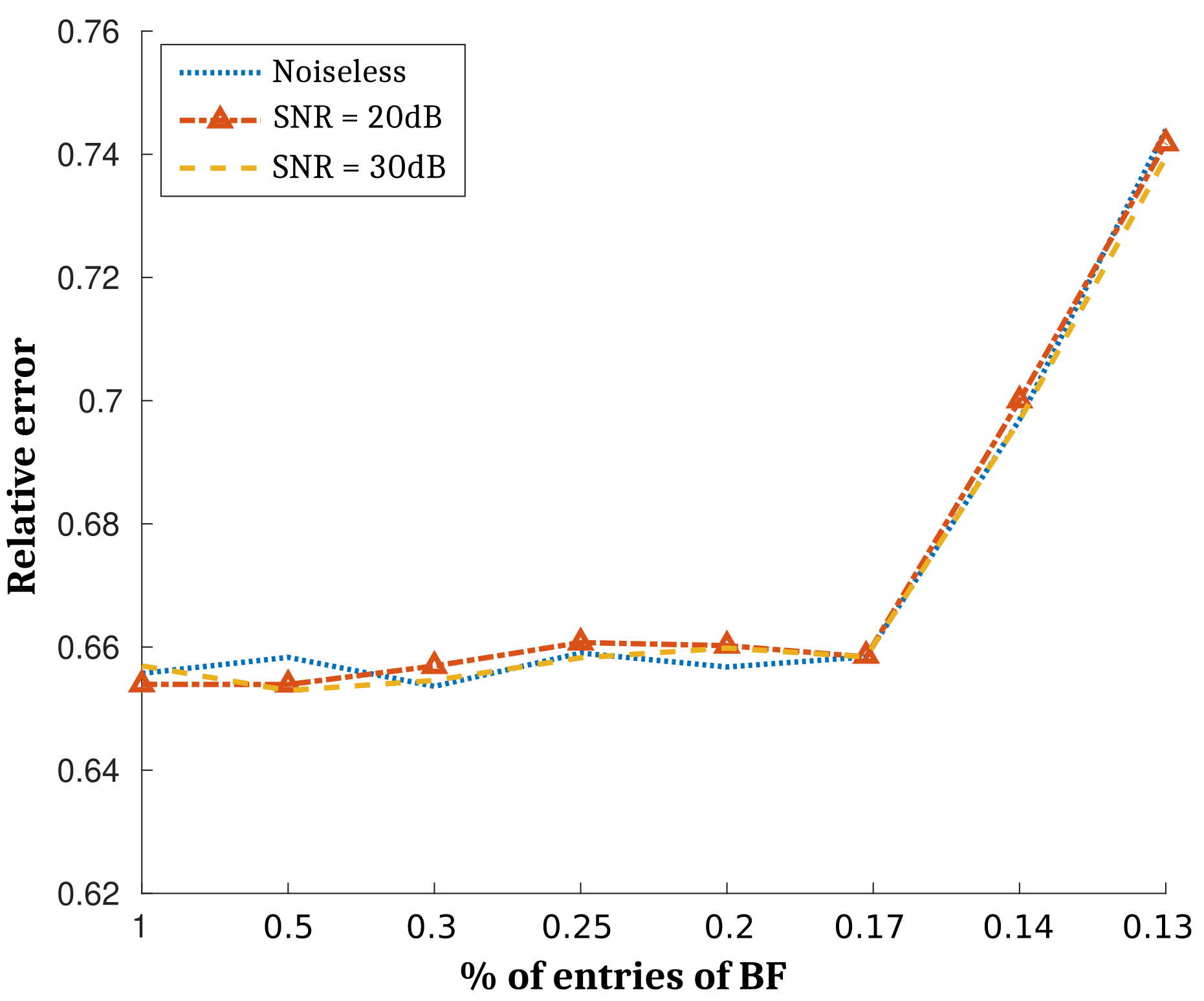
We examine the performance of vector $\boldsymbol{x}^{(0)}$ obtained by Algorithm 1 to approximate the pulse $\boldsymbol{x}$ with complete as well as sparse samples of the BF. We numerically determine the relative error averaged over 100 trials for both noiseless and noisy scenarios for SNR $=20$ and $30$ dB. Fig. 1 shows the effectiveness of Algorithm 1 to estimate the underlying pulse. To complement the numerical results in Fig. 1, we present the power spectrum estimate of $\boldsymbol{x}$. Fig. 2 shows an approximated version of $\lvert\boldsymbol{y}\rvert^{2}$ to visually illustrate the ability of Algorithm 1 to correctly estimate $\boldsymbol{y}$ while uniquely determining the roots of $\boldsymbol{s}[n]$ to approximate the underlying signal $\boldsymbol{x}$ even in the presence of Gaussian noise.

Finally, we evaluated the success rate of Algorithm 2 in Fig. 3. Here, Algorithm 2 is initialized at $\boldsymbol{x}^{(0)}=\boldsymbol{x}+\delta\zeta$, where $\delta$ is a fixed constant and $\zeta$ takes values on $\{-1,1\}$ with equal probability, while a percentage of the delays are set to zero. A trial is declared successful when the returned estimate attains a relative error that is smaller than $10^{-6}$. We numerically determine the empirical success rate among 100 trials. Fig. 3 shows that Algorithm 2 is able to estimate the pulse when the BF is incomplete.

We analytically demonstrated that band-limited signals can be estimated (up to trivial ambiguities) from its BF through our trust region gradient method. We evaluated our proposed technique for complete/incomplete noisy and noiseless scenarios. In the case of incomplete data, we found that although Proposition 1 suggests that the full BF is not required to guarantee uniqueness, there is potential to better estimate the pulses from incomplete data. Numerical experiments showed reasonably accurate performance for recovering both the magnitude and phase of the signal even from noisy incomplete data.

K. V. M. acknowledges partial support from the National Academies of Sciences, Engineering, and Medicine via the Army Research Laboratory Harry Diamond Distinguished Fellowship. Research was sponsored by the Army Research Laboratory and was accomplished under Cooperative Agreement Number W911NF-21-2-0288. The views and conclusions contained in this document are those of the authors and should not be interpreted as representing the official policies, either expressed or implied, of the Army Research Laboratory or the U.S. Government. The U.S. Government is authorized to reproduce and distribute reprints for Government purposes notwithstanding any copyright notation herein. S. P. acknowledges support from the EMET Research Institute in Colombia.

References

- [1] J. M. Mendel, “Tutorial on higher-order statistics (spectra) in signal processing and system theory: Theoretical results and some applications,” Proceedings of the IEEE, vol. 79, no. 3, pp. 278–305, 1991.
- [2] C. L. Nikias and J. M. Mendel, “Signal processing with higher-order spectra,” IEEE Signal Processing Magazine, vol. 10, no. 3, pp. 10–37, 1993.
- [3] K. V. Mishra, W. F. Krajewski, R. Goska, D. Ceynar, B.-C. Seo, A. Kruger, J. J. Niemeier, M. B. Galvez, M. Thurai, V. Bringi et al., “Deployment and performance analyses of high-resolution Iowa XPOL radar system during the NASA IFloodS campaign,” Journal of Hydrometeorology, vol. 17, no. 2, pp. 455–479, 2016.
- [4] V. Bringi, K. V. Mishra, M. Thurai, P. C. Kennedy, and T. H. Raupach, “Retrieval of lower-order moments of the drop size distribution using CSU-CHILL X-band polarimetric radar: A case study,” Atmospheric Measurement Techniques, vol. 13, no. 9, pp. 4727–4750, 2020.
- [5] K. Hood, S. Torres, and R. Palmer, “Automatic detection of wind turbine clutter for weather radars,” Journal of Atmospheric and Oceanic Technology, vol. 27, no. 11, pp. 1868–1880, 2010.
- [6] M. Thurai, K. V. Mishra, V. Bringi, and W. F. Krajewski, “Initial results of a new composite-weighted algorithm for dual-polarized X-band rainfall estimation,” Journal of Hydrometeorology, vol. 18, no. 4, pp. 1081–1100, 2017.
- [7] R. J. Doviak and D. S. Zrnić, Doppler Radar & Weather Observations, 2nd ed. Dover Publications, 2006.
- [8] P. V. Tryon, “The bispectrum and higher-order spectra: A bibliography,” National Bureau of Standards, Boulder, Colorado, USA, Technical Note 1036, 1981.
- [9] C. L. Nikias and M. R. Raghuveer, “Bispectrum estimation: A digital signal processing framework,” Proceedings of the IEEE, vol. 75, no. 7, pp. 869–891, 1987.
- [10] B. M. Sadler and G. B. Giannakis, “Shift-and rotation-invariant object reconstruction using the bispectrum,” Journal of the Optical Society of America A, vol. 9, no. 1, pp. 57–69, 1992.
- [11] M. D. Godfrey, “An exploratory study of the bi-spectrum of economic time series,” Journal of the Royal Statistical Society. Series C (Applied Statistics), vol. 14, no. 1, pp. 48–69, 1965.
- [12] K. Hasselmann, W. Munk, G. MacDonald, and M. Rosenblatt, “Bispectra of ocean waves,” in Proceedings of the Symposium on Time Series Analysis, M. Rosenblatt, Ed. John Wiley & Sons, 1963, pp. 125–139.
- [13] T. Sato and K. Sasaki, “Bispectral holography,” The Journal of the Acoustical Society of America, vol. 62, no. 2, pp. 404–408, 1977.
- [14] T.-W. Chen, W.-D. Jin, and J. Li, “Feature extraction using surrounding-line integral bispectrum for radar emitter signal,” in IEEE International Joint Conference on Neural Networks (IEEE World Congress on Computational Intelligence), 2008, pp. 294–298.
- [15] T. Matsuoka and T. J. Ulrych, “Phase estimation using the bispectrum,” Proceedings of the IEEE, vol. 72, no. 10, pp. 1403–1411, 1984.
- [16] J. Marron, P. Sanchez, and R. Sullivan, “Unwrapping algorithm for least-squares phase recovery from the modulo 2 bispectrum phase,” Journal of the Optical Society of America A, vol. 7, no. 1, pp. 14–20, 1990.
- [17] M. Rangoussi and G. B. Giannakis, “FIR modeling using log-bispectra: Weighted least-squares algorithms and performance analysis,” in International Conference on Acoustics, Speech, and Signal Processing, 1990, pp. 2399–2402.
- [18] D. R. Brillinger, “The identification of a particular nonlinear time series system,” Biometrika, vol. 64, no. 3, pp. 509–515, 1977.
- [19] K. Lii and M. Rosenblatt, “Deconvolution and estimation of transfer function phase and coefficients for nonGaussian linear processes,” The Annals of Statistics, vol. 10, no. 4, pp. 1195–1208, 1982.
- [20] H. Bartelt, A. W. Lohmann, and B. Wirnitzer, “Phase and amplitude recovery from bispectra,” Applied Optics, vol. 23, no. 18, pp. 3121–3129, 1984.
- [21] T. Bendory, N. Boumal, C. Ma, Z. Zhao, and A. Singer, “Bispectrum inversion with application to multireference alignment,” IEEE Transactions on Signal Processing, vol. 66, no. 4, pp. 1037–1050, 2017.
- [22] I. P. Theron, E. K. Walton, S. Gunawan, and L. Cai, “Ultrawide-band noise radar in the VHF/UHF band,” IEEE Transactions on Antennas and Propagation, vol. 47, no. 6, pp. 1080–1084, 1999.
- [23] C.-Y. Chen and P. P. Vaidyanathan, “MIMO radar space-time adaptive processing using prolate spheroidal wave functions,” IEEE Transactions on Signal Processing, vol. 56, no. 2, pp. 623–635, 2008.
- [24] S. Pinilla, K. V. Mishra, B. M. Sadler, and H. Arguello, “Phase retrieval for radar waveform design,” arXiv preprint arXiv:2201.11384, 2022.
- [25] S. Pinilla, K. V. Mishra, and B. Sadler, “WaveMax: FrFT-based convex phase retrieval for radar waveform design,” in IEEE International Symposium on Information Theory, 2021, pp. 2387–2392.
- [26] S. Pinilla, K. V. Mishra, B. M. Sadler, and H. Arguello, “BanRaW: Band-limited radar waveform design via phase retrieval,” in IEEE International Conference on Acoustics, Speech and Signal Processing, 2021, pp. 5449–5453.
- [27] H. Zhang and Y. Liang, “Reshaped Wirtinger flow for solving quadratic system of equations,” in Advances in Neural Information Processing Systems, 2016, pp. 2622–2630.
- [28] S. Pinilla, J. Bacca, and H. Arguello, “Phase retrieval algorithm via nonconvex minimization using a smoothing function,” IEEE Transactions on Signal Processing, vol. 66, no. 17, pp. 4574–4584, 2018.
- [29] J. Nocedal and S. Wright, Numerical optimization, 2nd ed. Springer, 2006.
- [30] J. C. Spall, Introduction to stochastic search and optimization: Estimation, simulation, and control. Wiley-Interscience, 2005.
- [31] R. S. Strichartz, A guide to distribution theory and Fourier transforms. World Scientific, 2003.