Floer-Novikov fundamental group and small flux symplectic isotopies

Jean-François Barraud Affiliation: Institut de Mathématiques de Toulouse ; UMR5219 Université de Toulouse ; CNRS. Agnès Gadbled Affiliation: Mathématiques Orsay; Université Paris Saclay ; CNRS.

Abstract

Floer theory relates the dynamics of Hamiltonian isotopies and the homology of the ambient manifold. It was extended to similarly relate the dynamics of symplectic isotopies and the Novikov homology associated to their flux. We discuss this picture regarding the fundamental group, and prove that when the flux is not too big, the associated Novikov fundamental group is generated by Floer moduli spaces associated to closed orbits of the symplectic isotopy.

1 Introduction and main statement

The celebrated Floer theory, introduced by Floer in [7, 6] as a tool to prove the Arnold conjecture, is designed to study fixed points of Hamiltonian isotopies or intersections of Lagrangian submanifolds under deformation by such isotopies, from an homological point of view. Among many other development of this theory, several authors [14],[12],[4],[9] extended his ideas to the case of symplectic (non Hamiltonian) isotopies, showing that the theory still makes sense, if the homology of the ambient manifold is replaced by the Novikov homology associated to the flux of the isotopy.

The goal of this paper is to study the same question from the fundamental group point of view. In the Hamiltonian setting, the Floer theory is rich enough to recover generators of the fundamental group of the ambient (closed and monotone) manifold as explained in [2]. On the other hand, to a degree $1$ cohomology class $[\alpha]$ on a closed manifold $M$ and a choice of integration cover $\tilde{M}$ for $[\alpha]$ is naturally associated a group $\pi_{1}(\tilde{M},[\alpha])$ , that generalizes the usual fundamental group to the Novikov setting, as explained in [3]. It is then natural to expect that the Floer construction adapts from the Hamiltonian to the symplectic case, replacing the fundamental group by the Novikov fundamental group.

The main theorem of this paper is to show that it is indeed the case for isotopies that have a small enough flux.

Consider a closed monotone symplectic manifold $(M,\omega)$ and a non degenerate symplectic isotopy $(\phi_{t})_{t\in[0,1]}$ . Let $X_{t}=\frac{d\phi_{t}}{dt}$ be the vector field generating this isotopy. The $1$ -form

\alpha_{\phi}=\int_{0}^{1}\omega(X_{t},\cdot)dt

is then closed, and its cohomology class $[\alpha_{\phi}]$ is called the flux of the isotopy (or its Calabi invariant [12]). This cohomology class only depends on the homotopy class of the path $(\phi_{t})$ with fixed ends.

Choose now an integration cover $\tilde{M}$ for $[\alpha_{\phi}]$ . There might be several possible choices, from the minimal one to the universal cover, and we fix one once for all (the resulting group we are about to define will depend on this choice, and each choice defines a different version of the invariant, just like in the case of Novikov homology).

Pick an $\omega$ compatible almost complex structure $J$ , which we allow to depend on two parameters $(s,t)\in[0,1]\times\mathbb{S}^{1}$ , and suppose it is chosen generic, meaning that all the relevant Floer theoretic moduli spaces are cutout transversely. Then a group $\mathop{\Omega}\nolimits(\phi,J)$ can be built out of theses moduli spaces with the following property :

Theorem 1.1.

Let $(M,\omega)$ be a closed monotone symplectic manifold and $(\phi_{t})$ a (non Hamiltonian) symplectic isotopy as above. If the flux $[\alpha_{\phi}]$ is small enough, then there is a surjective map

from $\mathop{\Omega}\nolimits(\phi,J)$ to the Novikov fundamental group associated to the flux of the isotopy.

Remark 1.

Notice that a small flux does not mean a small isotopy : Hamiltonian isotopies have a vanishing flux, but can still be arbitrary large.

Remark 2.

The construction relies on curves that are typically used to define the PSS morphism [13] between Floer and Morse homologies, and the key point is an energy/depth estimate for such curves to provide a control of such curves in the Novikov setting. In particular, the construction below could also provide a PSS morphism between the Floer to Morse Novikov homologies, as long as the flux of the symplectic isotopy used on the Floer side is small enough.

As an obvious corollary, we obtain a way to detect fixed points of symplectic isotopies.

Proposition 1.2.

In the situation of theorem 1.1, if $\pi_{1}(\tilde{M},[\alpha_{\phi}])\neq 1$ , then $\phi$ has fixed points.

Remark 3.

More explicit examples are easier to derive from the Lagrangian version…

1.1 Moduli spaces

Let $\mathcal{J}$ be the space of $\omega$ -compatible almost complex structures on $M$ that depend on two parameters $(s,t)\in[0,1]\times\mathbb{S}^{1}$ , and such that $J(0,t)$ is constant.

The main ingredient in the construction of the group of Floer loops $\mathop{\Omega}\nolimits(\phi,J)$ are the PSS-like moduli spaces

\mathcal{M}(y,\varnothing)

associated to an almost complex structure $J\in\mathcal{J}$ , i.e. moduli spaces of maps $u:\mathbb{R}\times\mathbb{S}^{1}\to\tilde{M}$ , with finite energy, that are solutions of the “truncated” Floer equation

\frac{\partial u}{\partial s}+J_{\chi(s),t}(u)\Big(\frac{\partial u}{\partial t}-\chi(s)X_{t}(u)\Big)=0.

(1)

Here, the cutoff function $\chi(s)$ is a smooth function such that $\chi(s)=1$ for $s\leq-1$ and $\chi(s)=0$ for $s\geq 0$ , and the almost complex structure $J$ is in fact the lift of $J$ to $\tilde{M}$ .

Solutions of this equation with finite energy do have limits at the ends, which are

•

a $1$ -periodic orbit $y$ of $X$ at $-\infty$ (in $\tilde{M}$ ),
•

an point $p\in\tilde{M}$ at $+\infty$ .

More precisely, we consider two lifts of the periodic orbits : first we consider $X$ as a vector field on $\tilde{M}$ , and the set $\mathcal{P}$ of its contractible periodic orbits consists of all the lifts of the contractible periodic orbits in $M$ . Second, we consider the covering $\tilde{\mathcal{P}}$ of $\mathcal{P}$ obtained by considering discs bounded by periodic orbits under the equivalence relation :

\gamma\sim\gamma^{\prime}\iff\omega(\gamma)=\omega(\gamma^{\prime})\text{ and }\mu_{CZ}(\gamma)=\mu_{CZ}(\gamma^{\prime}),

where $\mu_{CZ}$ denotes the Conley Zehnder index. From now on, we will avoid stressing the use of these coverings all along the paper, and when speaking of a “periodic orbits of $X$ ”, we will in fact refer to an element in $\tilde{\mathcal{P}}$ .

In particular, in the situation above, the curve $u$ defines a disc bounded by the periodic orbit at $-\infty$ , and we will see the limit $y$ as an element of $\tilde{\mathcal{P}}$ rather than $\mathcal{P}$ .

For convenience, we will use the following shifted index rather than the Conley Zehnder index on $\tilde{\mathcal{P}}$ :

|y|=\mu_{CZ}(y)+n

(where $n=\frac{1}{2}\dim(M)$ ). Then, for a generic choice of $J$ , the moduli space $\mathcal{M}(y,\varnothing)$ is a smooth manifold and

\dim\mathcal{M}(y,\varnothing)=|y|.

We are interested in the connected components of such $1$ dimensional moduli spaces.

Compactification of bounded ends

Consider a connected component of $\mathcal{M}(y,\varnothing)$ for some periodic orbit $y$ such that $|y|=1$ . We are interested in the case when it is not closed (i.e.compact without boundary). Since it is a one dimensional manifold, it has two ends, each of them being homeomorphic to a half line $[0,\infty)$ .

•

If the energy is bounded on an end : it is said to be a bounded end, and it can be compactified by adding a broken configuration $(u,v)\in\mathcal{M}(y,x)\times\mathcal{M}(x,\varnothing)$ through an intermediate orbit $x$ with $|x|=0$ .
•

Otherwise it is said to be an unbounded end.

From now on, $\mathcal{M}(y,\varnothing)$ will denote the moduli space with compactified bounded ends.

The minimal requirement to control the unbounded ends is to show that some notion of depth is proper on $\mathcal{M}(y,\varnothing)$ , which is the object of the next section.

Refer to caption — Figure 1: Bounded and unbounded ends in $\mathcal{M}(y,\varnothing)$ .

2 Energy/depth estimates

Let $H_{t}:\tilde{M}\to\mathbb{R}$ be a Hamiltonian on $\tilde{M}$ generating the isotopy i.e. such that

dH_{t}=-\omega(X_{t},\cdot).

We use the deformation lemma from [12, lemma 2.1, p.157], to modify the isotopy, keeping its ends fixed, so that the cohomology class $[-\omega(X_{t},\cdot)]$ is in fact constant equals to the flux $[\alpha]$ .

We pick a primitive $\tilde{M}\xrightarrow{f}\mathbb{R}$ of $\pi^{*}\alpha$ . We will refer to the values of $f$ at a point $p$ as its height in $\tilde{M}$ with respect to $[\alpha]$ .

Notice that $dH_{t}-df$ descends to $M$ as an exact form, so that there is a constant $K$ such that

\|H-f\|_{\infty}\leq K.

(2)

2.1 Average depth estimate

Let $u\in\mathcal{M}(y,\varnothing)$ be a solution of the truncated Floer equation (1) as above.

Recall that the energy of $u$ is

E(u)=\iint||\frac{\partial u}{\partial s}||^{2}dsdt.

The following straightforward computation:

$\displaystyle E(u)$	$\displaystyle=\iint\omega(\frac{\partial u}{\partial s},J\frac{\partial u}{\partial s})dsdt$
	$\displaystyle=\iint\omega(\frac{\partial u}{\partial s},\frac{\partial u}{\partial t})dsdt-\iint\omega(\frac{\partial u}{\partial s},X)\chi(s)dsdt$
	$\displaystyle=\iint u^{*}\omega dsdt-\iint dH_{t}(\frac{\partial u}{\partial s})\chi(s)dsdt$
	$\displaystyle=\iint u^{*}\omega dsdt-\int[H_{t}(u)\chi(s)]_{s=-\infty}^{s=+\infty}+\iint H_{t}(u)\chi^{\prime}(s)dsdt$
	$\displaystyle=\iint u^{*}\omega dsdt+\int H_{t}(y(t))dt+\iint H_{t}(u)\chi^{\prime}(s)dsdt$
	$\displaystyle=\mathcal{A}(y)-\iint H_{t}(u)\|\chi^{\prime}(s)\|dsdt$	(3)

shows that for a fixed action $\mathcal{A}(y)$ , the energy is related to the average of $H$ in the cutoff region $\{-1\leq s\leq 0\}\times\mathbb{S}^{1}$ with respect to the measure $|\chi^{\prime}(s)|dsdt$ , and hence to the average depth of $u$ in this region.

However, we want to evaluate one dimensional moduli spaces as paths in $\tilde{M}$ and keep control of the depth along such paths : this requires point-wise estimates that cannot be directly derived from the above average estimate in general.

The object of the next section is to obtain such a point-wise estimate when the flux is not too big, based on the monotonicity principle and the Schwarz lemma for pseudo-holomorphic curves observed by Gromov in [11].

Before proceeding, we need to upgrade the average depth estimate (3) on the region $-1\leq s\leq 0$ into estimates that are pointwise with respect to $s$ .

Namely, let

m(s)=\int_{0}^{1}H_{t}(u(s,t))dt

Then $m^{\prime}(s)=\int_{0}^{1}\omega(\frac{\partial u}{\partial s},X)dt$ , and for $s_{0}\leq s_{1}$ we have :

	$\displaystyle m(s_{1})-m(s_{0})$	$\displaystyle=\int_{s=s_{0}}^{s=s_{1}}\int_{t=0}^{t=1}\omega(\frac{\partial u}{\partial s},X)dtds$
		$\displaystyle=\iint_{s_{0}\leq s\leq s_{1}}<\frac{\partial u}{\partial t},X>-\chi\\|X\\|^{2}dtds$
		$\displaystyle\leq\left(\iint_{s_{0}\leq s\leq s_{1}}\\|\frac{\partial u}{\partial t}\\|^{2}dsdt\right)^{1/2}\left(\iint_{s_{0}\leq s\leq s_{1}}\\|X\\|^{2}dsdt\right)^{1/2}$
		$\displaystyle\leq\sqrt{E(u)}\ \sqrt{s_{1}-s_{0}}\ \\|X\\|_{\infty}$

where $\|X\|_{\infty}=\sup\{\omega(X_{t}(p),J_{s,t}X_{t}(p)),(s,t)\in[0,1]\times\mathbb{S}^{1},p\in M\}$ . On the other hand, from (3), there is at least one $s_{0}\in[-1,0]$ such that $m(s_{0})=\mathcal{A}(y)-E(u)$ . This implies that for $s\geq 0$ we have :

\int_{0}^{1}H_{t}(u(s,t))dt\leq-E(u)+\|X\|_{\infty}\sqrt{s+1}\sqrt{E(u)}+\mathcal{A}(y)

(4)

and hence, letting $\sigma_{u}=\frac{E(u)}{4\|X\|^{2}}-1$ , we have for all $s\in[0,\sigma_{u}]$ :

\forall s\in[0,\sigma_{u}]:\ \int_{0}^{1}H_{t}(u(s,t))dt\leq-\frac{E(u)}{2}+\mathcal{A}(y).

(5)

2.2 Depth estimate at $+\infty$ .

On the line $\mathbb{R}[\alpha]$ , we pick a generator $[\alpha_{0}]$ , and a primitive $f_{0}$ of a form $\alpha_{0}$ in this class. We define $\lambda$ as

[\alpha]=\lambda[\alpha_{0}]

(6)

Let $\delta_{0}$ be a non trivial period of $[\alpha_{0}]$ (i.e. a positive real number such that there is some $g\in\pi_{1}(M)$ with $\alpha_{0}(g)=\delta_{0}$ ), and consider the slice

S=f_{0}^{-1}([0,\delta_{0}])\subset\tilde{M}

Notice that $\tilde{M}$ is a union of copies of this slice under deck transformations.

The main remark we’ll make use of to relate the depth at $u(+\infty)$ and the energy of our curves is that holomorphic curves need a minimal energy to go through a slice. This is a direct consequence of the monotonicity principle for $J$ -holomorphic curves described by Gromov [11]. However, since our curves are not everywhere holomorphic, we will also need to study the behavior of curves for which transition region between the Floer and the purely holomorphic areas is stretched across a large height.

2.2.1 Energy of holomorphic discs with low boundary and high center

First recall the crucial monotonicity principle for $J$ holomorphic curves, due to M. Gromov.

Lemma 2.1.

Given an $\omega$ compatible almost complex structure $J$ , there are constants $r_{0}$ and $C$ such that, for every $r\in(0,r_{0}]$ , for every point $x\in\tilde{M}$ and every $J$ -holomorphic map $u:\Sigma\to\tilde{M}$ defined on a Riemann surface $\Sigma$ such that

•

$u(\Sigma)\subset B(x,r)$ ,
•

$u(\partial\Sigma)\subset\partial B(x,r)$
•

$u$ goes through the center of the ball,

then $\iint_{\Sigma}u^{*}\omega\geq Cr^{2}$

A direct consequence of the monotonicity principle is that holomorphic curves that go across a slice $S$ of $\tilde{M}$ have a symplectic area bounded from below.

Lemma 2.2.

There are constants $K_{1}$ and $K_{2}$ (depending only on $M$ , $\omega$ , $J$ , $\Xi_{0}$ but not on $\lambda$ , $X$ or $H$ ) such that, for every $u\in\mathcal{M}(y,\varnothing)$ and every $s_{0}\geq 0$ :

E(u)\geq\frac{K_{1}}{\lambda}\Big(f(u(+\infty))-\max_{\{s=s_{0}\}}(f(u))\Big)-K_{2}

(7)

Proof.

Recall we let $S=f_{0}^{-1}([0,\delta_{0}])$ , and consider $S^{\prime}=f_{0}^{-1}([\frac{\delta_{0}}{3},\frac{2\delta_{0}}{3}])$ . Recall that the almost complex structure $J(s,t)$ is in fact constant for $s\geq 0$ , and consider a radius $r_{0}$ and a constant $C$ associated to this almost complex structure by lemma2.1. Pick a radius $R\leq r_{0}$ such that at every point $p\in S^{\prime}$ , the $R$ -ball at $p$ is contained in $S$ .

The holomorphic disc $u_{|_{\{s\geq s_{0}\}}}$ has to cross at least $N$ copies of $S$ where

N=\left\lfloor\frac{f_{0}(u(0))-\max_{\{s=s_{0}\}}(f_{0}(u))}{\delta_{0}}\right\rfloor-2.

For each copy $S_{i}$ of $S$ , pick an $R$ -ball centered at a point $p_{i}=u(z_{i})\in S^{\prime}_{i}$ for $z_{i}\in D$ : from lemma 2.1, we obtain

E(u)\geq NCR^{2}

which leads to the desired estimate. ∎

2.2.2 Upper bounds for the height on the transition annulus.

For a curve $u\in\mathcal{M}(y,\varnothing)$ , recall the notation $\sigma_{u}=\frac{E(u)}{4\|X\|^{2}}-1$ from (5), and consider the annulus

A_{u}=[0,\sigma_{u}]\times\mathbb{S}^{1}.

We now want to prove that the annulus $A_{u}$ does indeed contain a loop $\{s=cst\}$ that does not go above a deep level :

Lemma 2.3.

There is a constant $K_{3}$ (depending on $M$ , $\omega$ , $J$ , $\phi$ ) such that, for every $u\in\mathcal{M}(y,\varnothing)$ , there is some $s_{0}\geq 0$ such that

\max_{t\in\mathbb{S}^{1}}\{f(u(s_{0},t))\}\leq\mathcal{A}(y)-\frac{E(u)}{2}+K_{3}

Let

\Delta_{f}(s)=\max_{t\in\mathbb{S}^{1}}f(u(s,t))-\min_{t\in\mathbb{S}^{1}}f(u(s,t))

(8)

and consider a point $s_{0}\in[0,\sigma_{u}]$ where this magnitude is minimal :

\Delta_{f}(s_{0})=\min_{s\in[0,\sigma_{u}]}\Delta_{f}(s).

Recall that $|f-H|$ is uniformly bounded on $\tilde{M}$ . Using (5) in the last line of the following estimates

	$\displaystyle\max_{t\in\mathbb{S}^{1}}f(u(s_{0},t))$	$\displaystyle\leq\int_{0}^{1}f(u(s,t))dt+\Delta_{f}(s_{0})$
		$\displaystyle\leq\int_{0}^{1}H_{t}(u(s,t))dt+\\|f-H\\|_{\infty}+\Delta_{f}(s_{0})$
		$\displaystyle\leq\mathcal{A}(y)-\frac{E(u)}{2}+\\|f-H\\|_{\infty}+\Delta_{f}(s_{0}),$

we obtain that the proof of lemma 2.3 reduces to the following lemma :

Lemma 2.4.

There is a uniform constant $K_{3}$ (depending on $M$ , $\omega$ , $J$ , $[\alpha]$ and $\phi$ ), such that for all $u\in\mathcal{M}(y,\varnothing)$ :

\min_{s\in[0,\sigma_{u}]}\Delta_{s}f(u)\leq K_{3}

(9)

We will need the classical Gromov-Schwarz lemma, which is a consequence of the monotonicity principle. The following form is again picked from [1, p.181] :

Lemma 2.5.

Given an $\omega$ -compatible almost complex structure $J$ that may depend on a parameter in the unit disc, there is a constant $C$ such that, for every map $u:D\to\tilde{M}$ defined on the unit disc such that

•

$u$ is $J$ -holomorphic in $D$ ,
•

$\iint_{D}u^{*}\omega\leq a_{0}$ ,

then $\|d_{0}u\|\leq C$ .

Proof of lemma 2.4.

For all $s\in[0,\sigma_{u}]$ , we have

\max_{t\in\mathbb{S}^{1}}(f(u(s,t)))-\min_{t\in\mathbb{S}^{1}}(f(u(s,t)))\geq\Delta_{f}(s_{0}),

so that above each $s\in[0,\sigma_{u}]$ there is a point $z_{s}=s+it_{s}$ such that

\|du(z_{s})\|\geq\frac{\Delta_{f}(s_{0})}{\|df\|_{\infty}}

Let $r=\frac{\|df\|_{\infty}}{\Delta_{f}(s_{0})}\,C$ (where $C$ is the constant appearing in the Gromov-Schwarz lemma 2.5), and consider the $r$ -subdivision $(s_{1},\dots,s_{N})$ given by

s_{k}=k\,r,\quad 1\leq k\leq N\ \text{ with }\ N=\left\lfloor\frac{\sigma_{u}}{r}\right\rfloor

The associated points $z_{k}=s_{k}+it_{s_{k}}$ are such that :

r\|du(z_{k})\|\geq C

and hence, from lemma 2.5:

\iint_{D(z_{k},r)}u^{*}\omega\geq a_{0}.

Because the discs $D(z_{k},r)$ are all disjoint, we obtain

\displaystyle E(u)

\displaystyle\geq Na_{0}\geq(\frac{\sigma_{u}}{r}-1)a_{0}=\left(\frac{\sigma_{u}\,\Delta_{s_{0}}f(u)}{C\|df\|_{\infty}}-1\right)a_{0}

Recalling that $\sigma_{u}=\frac{E(u)}{4\|X\|^{2}}$ , this means that

\Delta_{s_{0}}f(u)\leq\frac{4C\|X\|^{2}\|df\|_{\infty}}{a_{0}}\left(\frac{E(u)+a_{0}}{E(u)}\right),

which leads to the desired result when $E(u)\geq 1$ . On the other hand, if $E(u)\leq 1$ , $u$ belongs to a compact subset of the moduli space, on which the maximal and minimal height, and hence a fortiori $\Delta_{s_{0}}f(u)$ , have to be bounded. ∎

2.2.3 Depth estimate at $+\infty$ .

Recall from (6) the definition of $\lambda$ by the relation

[\alpha]=\lambda[\alpha_{0}].

Lemma 2.6.

There is a positive constant $A$ depending only on $M$ , $\omega$ , $J$ and $[\alpha_{0}]$ (but not on $\lambda$ ), and a constant $B$ that may depend also on $\lambda$ and $\phi$ , such that for all maps $u\in\mathcal{M}(y,\varnothing)$ :

f(u(+\infty))\leq\mathcal{A}(y)-(\frac{1}{2}-A\lambda)E(u)+B

In particular, for $\lambda<\frac{1}{2A}$ , we have

\lim_{E(u)\to+\infty}f(u(+\infty))=-\infty.

Proof.

From lemma 2.3, there is some $s_{0}$ such that

\max_{t\in\mathbb{S}^{1}}\{f(u(s_{0},t))\}\leq\mathcal{A}(y)-\frac{E(u)}{2}+K_{3}

On the other hand, from lemma 2.2, we have

	$\displaystyle f(u(+\infty))$	$\displaystyle\leq\frac{\lambda(E(u)+K_{2})}{K_{1}}+\max_{t\in\mathbb{S}^{1}}\{f(u(s_{0},t))\}$
		$\displaystyle\leq\mathcal{A}(y)-\Big(\frac{1}{2}-\frac{\lambda}{K_{1}}\Big)E(u)+\lambda\frac{K_{2}}{K_{1}}+K_{3},$

which ends the proof since $K_{1}$ is independent of $\lambda$ .

∎

Notice for future use that the same argument applies when the roles of the ends in the Floer equation are flipped. We denote by $\mathcal{M}(\varnothing,y)$ the corresponding space. Then we have the following lemma :

Lemma 2.7.

There is positive constant $A$ depending only on $M$ , $\omega$ , $J$ and $[\alpha_{0}]$ (but not on $\lambda$ ) and a constant $B$ that may depend also on $\lambda$ and $\phi$ , such that, for all maps $u\in\mathcal{M}(\varnothing,y)$ :

f(u(+\infty))\geq\mathcal{A}(y)+(\frac{1}{2}-\lambda A)E(u)-B.

In particular, for $\lambda<\frac{1}{2A}$ , we have

\lim_{E(u)\to+\infty}f(u(-\infty))=+\infty.

3 Floer Novikov loops for small flux

We now restrict to symplectic isotopies that have a small enough flux, namely such that $\lambda<\frac{1}{2A}$ with the notation of lemma 2.6, so that the map

\begin{array}[]{ccc}\mathcal{M}(y,\varnothing)&\xrightarrow{f\circ\mathrm{ev}}&\mathbb{R}\\ u&\mapsto&f(u(+\infty))\end{array}

is proper on all the moduli spaces $\mathcal{M}(y,\varnothing)$ . From now on, the depth of a curve $u$ will refer to the depth $f(u(+\infty))$ of the point $u(\infty)$ .

3.1 Definition of Floer Novikov loops

The definition of Floer-Novikov loops mimics the definition of Morse-Novikov loops given in [3]. We let

\mathcal{M}(y,\{f\geq h\})=\{u\in\mathcal{M}(y,\varnothing),f(u(+\infty))\geq h\}

For a generic choice of the level $h$ , this is a one dimensional manifold with boundary, and its boundary is given either by Floer breaks or by the condition $f(u(+\infty))=h$ .

Definition 3.1.

A Floer-Novikov step relative to $h$ is a connected component of a $1$ dimensional moduli space $\mathcal{M}(y,\{f\geq h\})$ with non empty boundary, endowed with an orientation.

Remark 4.

In this definition all the components of $\mathcal{M}(y,\{f\geq h\})$ are considered separately. Another choice would be to concatenate all such components that belong to the same component of $\mathcal{M}(y,\varnothing)$ . We will see below that the two choices eventually lead to the same group.

Remark 5.

This definition obviously depends on the choice of the function $f$ used to measure the “depth”, but it will be rather obvious that the resulting defintion of the Floer Novikov fundamental group will not.

According to its orientation, a step $\sigma$ has a starting and an ending level, which is either $h$ or $f(v(+\infty))$ if the corresponding end is a broken configuration $(u,v)\in\mathcal{M}(y,x)\times\mathcal{M}(x,\varnothing)$ .

It also has a highest level which is the highest depth $f(u(+\infty))$ over all curves $u$ in the step.

Definition 3.2.

Fix a level $h\in\mathbb{R}$ . Two Floer Novikov steps $\sigma_{1}$ and $\sigma_{2}$ are said to be consecutive if either :

•

$\sigma_{1}$ ends and $\sigma_{2}$ starts on the level $h$ ,
•

or $\sigma_{1}$ ends and $\sigma_{2}$ starts with broken configurations that involve the same orbit $x$ and the same curve $v\in\mathcal{M}(x,\varnothing)$ .

A Floer-Novikov loop relative to $h$ is then a sequence of consecutive steps, the first starting and the last ending on the level $h$ .

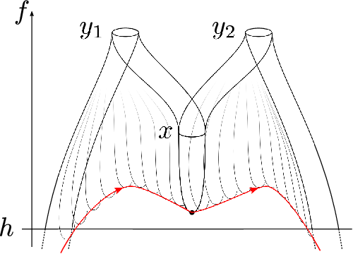
The obvious concatenation rule and the equivalence relation $\sim$ induced by cancellation of the occurrence of two consecutive copies of the same step with opposite orientations turns the collection of all loops relative to $h$ into a group, that will be denoted by

\lfloor\mathop{\Omega}\nolimits(\tilde{M},J,\phi)\rfloor_{h}.

Moreover, given two levels $h^{\prime}<h$ , loops relative to $h^{\prime}$ are a fortiori loops relative to $h$ , and there is a natural restriction map

\lfloor\mathop{\Omega}\nolimits(\tilde{M},J,\phi)\rfloor_{h^{\prime}}\xrightarrow{\zeta_{h^{\prime}}^{h}}\lfloor\mathop{\Omega}\nolimits(\tilde{M},J,\phi)\rfloor_{h}.

Finally, given three levels $h^{\prime\prime}<h^{\prime}<h$ , we have $\zeta_{h^{\prime}}^{h}\circ\zeta_{h^{\prime\prime}}^{h^{\prime}}=\zeta_{h^{\prime\prime}}^{h}$ .

Definition 3.3.

Define the group of Floer Novikov loops as

\mathop{\Omega}\nolimits(\tilde{M},J,\phi)=\varprojlim\lfloor\mathop{\Omega}\nolimits(\tilde{M},J,\phi)\rfloor_{h}.

For convenience, we may omit the dependency on $\tilde{M}$ and $J$ in the notation.

Remark 6.

Since the difference between two choices of height functions is always bounded, it is not hard to see that the direct limit process discards all dependency on this choice.

3.1.1 Full Floer Novikov steps

A component $\sigma$ of $\mathcal{M}(y,\varnothing)$ , when restricted above a level $h$ , defines a sequence of components in $\mathcal{M}(y,\{f\geq h\})$ , i.e. a sequence of steps, that are obviously consecutive. We call this concatenation of all the Floer steps that come from the same component of $\mathcal{M}(y,\varnothing)$ a full Floer Novikov step.

Definition 3.4.

A full Floer step above a given level $h$ is the concatenation of all the Floer steps relative to $h$ that belong to the same component $\sigma\subset\mathcal{M}(y,\varnothing)$ , in the order given by this component.

We denote by $\lfloor\mathop{\Omega}\nolimits^{\prime}(\phi)\rfloor_{h}$ the associated space of loops (i.e. sequences of consecutive full steps, the first starting and the last ending on level $h$ ) and let

\mathop{\Omega}\nolimits^{\prime}(\phi)=\varprojlim_{h}\lfloor\mathop{\Omega}\nolimits^{\prime}(\phi)\rfloor_{h}.

Notice that $\lfloor\mathop{\Omega}\nolimits^{\prime}{\phi}\rfloor_{h}$ is a subgroup of $\lfloor\mathop{\Omega}\nolimits{\phi}\rfloor_{h}$ , and the restriction maps induce an inclusion in the limit.

\mathop{\Omega}\nolimits^{\prime}{\phi}\hookrightarrow\mathop{\Omega}\nolimits{\phi}.

Proposition 3.5.

The loops groups generated by full or regular Floer steps are the same :

\mathop{\Omega}\nolimits^{\prime}{\phi}=\mathop{\Omega}\nolimits{\phi}.

In other words, using the terminology of [3], the collection of all the components of all the moduli spaces $\mathcal{M}(y,\varnothing)$ generate $\mathop{\Omega}\nolimits(\phi)$ up to deck transformations and completion.

This is a consequence of lemma 3.6 below, which itself is a direct consequence of the properness of the map $u\mapsto f(u(+\infty))$ .

Lemma 3.6.

For every $\Delta^{+}>0$ , there is a constant $\Delta^{-}>0$ such that for every levels $h$ and $h^{\prime}$ with $h^{\prime}\leq h-\Delta^{-}$ , and every index $1$ orbit $y$ with $\mathcal{A}(y)\leq h+\Delta^{+}$ , two components of $\mathcal{M}(y,\{f\geq h\})$ that belong to the same component of $\mathcal{M}(y,\varnothing)$ belong to the same component of $\mathcal{M}(y,\{f\geq h^{\prime}\})$ .

Proof.

If this is not the case, we find a constant $\Delta^{+}$ and a sequence $h_{n}$ , $h^{\prime}_{n}$ , $y_{n}$ such that

1.

$\mathcal{A}(y_{n})\leq h_{n}+\Delta^{+}$ ,
2.

$h^{\prime}_{n}<h_{n}-n$ ,

and two disjoint components $\sigma^{\prime}_{n,1}$ and $\sigma^{\prime}_{n,2}$ of $\mathcal{M}(y,\{f\geq h^{\prime}_{n}\})$ that belong to the same component of $\mathcal{M}(y,\varnothing)$ such that $\sigma^{\prime}_{n,i}\cap\mathcal{M}(y,\{f\geq h_{n}\})\neq\varnothing$ for $i=1,2$ .

Up to a sub-sequence and shifts in $\tilde{M}$ , the orbit $y_{n}$ can be supposed to be in fact a constant orbit $y$ . The sequence $h_{n}$ is then bounded from below, and can also be supposed to be constant without loss of generality.

For $i=1,2$ , pick some $u_{n,i}\in\sigma^{\prime}_{n,i}\cap\mathcal{M}(y,\{f\geq h_{n}\})$ . Since $\mathcal{M}^{\geq h}(y,\varnothing)$ is compact, both sequences $(u_{n,1})$ and $(u_{n,2})$ and can be supposed to converge, and hence to be constant.

Since $u_{1}$ and $u_{2}$ belong to the same component of $\mathcal{M}(y,\varnothing)$ which is $1$ dimensional, they bound a compact segment $[u_{1},u_{2}]$ in $\mathcal{M}(y,\varnothing)$ . On the other hand, since this segment cannot is not fully contained in $\mathcal{M}(y,\{f\geq h^{\prime}_{n}\})$ by assumption, there is a point $v_{n}$ between $u_{1}$ and $u_{2}$ such that $f(v_{n}(+\infty))<h^{\prime}_{n}$ . In particular

\lim f(v_{n}(+\infty))=-\infty,

which contradicts the compactness of $[u_{1},u_{2}]$ . ∎

Proof of proposition 3.5.

Pick an element $\gamma\in\mathop{\Omega}\nolimits(\phi)$ , and a level $h$ . Consider the reduced word representing $\zeta_{-\infty}^{h}(\gamma)$ : it is a finite sequence $(\sigma_{1},\dots,\sigma_{k})$ of components of moduli spaces $\mathcal{M}(y_{i},\{f\geq h\})$ .

Let $\mathcal{A}_{\max}=\max\{\mathcal{A}(y_{i})\}$ , and consider the level $h^{\prime}=h-\Delta^{-}$ where $\Delta^{-}$ is the constant provided by lemma 3.6 when taking $\Delta^{+}=\mathcal{A}_{\max}-h$ .

Then $\zeta_{-\infty}^{h}(\gamma)=\zeta_{h^{\prime}}^{h}(\zeta_{-\infty}^{h^{\prime}}(\gamma))$ . This means that the components $\sigma_{i}$ are restriction above level $h$ of components of $\mathcal{M}(y,\{f\geq h^{\prime}\})$ : from lemma 3.6, this means they are in fact full Floer steps. ∎

3.2 Evaluation

Notice that the evaluation at $+\infty$ , denoted as

\mathcal{M}(y,\varnothing)\xrightarrow{\mathrm{ev}}\tilde{M},

continuously extends to the broken configurations. It turns each component of $\mathcal{M}(y,\varnothing)$ into a path in $\tilde{M}$ that is well defined up to parameterization, and for which unbounded ends go to $-\infty$ in $\tilde{M}$ .

Focusing on subs-levels and passing to homotopy classes, we get rid of the parameterization ambiguity and obtain a well defined maps

\lfloor\mathop{\Omega}\nolimits(\tilde{M},J,\phi)\rfloor_{h}\xrightarrow{\mathrm{ev}}\lfloor\pi_{1}(\tilde{M},\alpha)\rfloor_{h}

for every levels $h\in\mathbb{R}$ . For $h^{\prime}<h$ they make the following diagram commutative :

In particular, these evaluation maps induce a map in the limit :

\mathop{\Omega}\nolimits(\tilde{M},J,\phi)\xrightarrow{\mathrm{ev}}\pi_{1}(\tilde{M},\alpha).

(10)

The main result in this paper is the following:

Theorem 3.7.

Consider a non degenerate symplectic isotopy $\phi$ in $M$ and equip $M$ with a generic almost complex structure $J\in\mathcal{J}$ . If the flux of $\phi$ is small enough, then the evaluation map

\mathop{\Omega}\nolimits(\tilde{M},J,\phi)\xrightarrow{\mathrm{ev}}\pi_{1}(\tilde{M},\alpha)

is onto.

The proof of this theorem reduces to prove that any Morse Novikov loop is homotopic to Floer Novikov loop, which is the object of the next section.

4 From Morse Novikov to Floer Novikov loops

In this section, we suppose that the $1$ -form picked in the cohomology class $[\alpha]$ to define the depth function $f$ is Morse, so that the function $f$ itself is Morse on $\tilde{M}$ . Moreover, as $[\alpha]\neq 0$ , we can also suppose for convenience that $f$ has no index $0$ critical point.

We also pick a Riemannian metric $<,>$ on $M$ , that we lift to $\tilde{M}$ , such that the pair $(f,<,>)$ is Morse Smale on $\tilde{M}$ . In this situation, the unstable manifold of a critical point $b$ of index $1$ of $f$ is a path $\gamma_{b}$ going to $-\infty$ on both ends in $\tilde{M}$ . We call the restriction of such a path above a level $h$ a Morse-Novikov step relative to $h$ , and define the space of Morse-Novikov $\mathop{\Omega}\nolimits(f)$ in the same way as before. In this simplified situation, this sums up to letting : $\mathop{\Omega}\nolimits(f)=\varprojlim_{h}\lfloor\mathop{\Omega}\nolimits(f)\rfloor_{h}$ where

\lfloor\mathop{\Omega}\nolimits(f)\rfloor_{h}=<b\in\mathrm{Crit}_{1}(f)\ |\ b=1\text{ if }f(b)\leq h>

is the group freely generated by the index $1$ critical points $b$ of $f$ where $f(b)\geq h$ .

Finally, recall from [3] that the natural evaluation map to the Novikov fundamental group

\mathop{\Omega}\nolimits(f)\xrightarrow{\mathrm{ev}}\pi_{1}(\tilde{M},[\alpha])

is surjective.

The object of this section is to prove the following proposition :

Proposition 4.1.

The above evaluation map factors through $\mathop{\Omega}\nolimits(\phi)$ , i.e. there is a group morphism $\psi$ making the following diagram commutative :

In particular, the evaluation $\mathop{\Omega}\nolimits(\phi)\to\pi_{1}(\tilde{M},\Xi)$ is surjective.

To associate a Floer-Novikov loop to a Morse-Novikov loop, we will make use of hybrid moduli spaces, that are built out of the space $\mathcal{M}(\varnothing,\varnothing)$ of solutions, in the trivial homotopy class, of the Floer equation in which the Hamiltonian term is truncated at both ends. More precisely, this equation is the following :

\frac{\partial u}{\partial s}+J_{\chi(s),t}(u)\Big(\frac{\partial u}{\partial t}-\chi_{R}(s)X_{t}(u)\Big)=0.

(11)

where

\chi_{R}(s)=\chi(s-R)\chi(-s-R)

is a smooth function such that $\chi_{R}(s)=1$ for $|s|\leq R-1$ and $\chi_{R}(s)=0$ for $|s|\geq R$ . Here $R$ is a non negative number that is part of the unknown.

A solution $(u,R)$ of this equation with finite energy has limits at both ends ends, which are just points in $\tilde{M}$ . In particular, it induces a map from $\mathbb{S}^{2}$ to $\tilde{M}$ . We denote by $\mathcal{M}(\varnothing,\varnothing)$ the space of couples $(u,R)$ satisfying (12) such that

1.

$u$ has finite energy,
2.

as a map from $\mathbb{S}^{2}$ to $\tilde{M}$ , $u$ is in the trivial homotopy class.

For a generic choice of $J$ this is a smooth manifold with boundary, of dimension $n+1$ . The boundary is given by the condition $R=0$ , and consists in the constant maps $u:\mathbb{R}\times\mathbb{S}^{1}\to\tilde{M}$ .

The energy sub-levels are compact up to breaks, and we still denote the space obtained by compactifying all the energy sub-levels by $\mathcal{M}(\varnothing,\varnothing)$ .

Given an index $1$ critical point $b$ of $f$ , the hybrid spaces we are interested in are the following :

\mathcal{M}(b,\varnothing)=\{(u,R)\in\mathcal{M}(\varnothing,\varnothing),u(-\infty)\in W^{u}(b)\}

and

\mathcal{M}(b,\{f\geq h\})=\{(u,R)\in\mathcal{M}(b,\varnothing),f(u(+\infty))\geq h\}.

To control the compactness of such spaces with respect to depth, we again need an energy-depth estimate for them, which is the object of the next section.

4.1 Energy/depth estimate on $\mathcal{M}(\varnothing,\varnothing)$

The same computations as for the augmentation curves shows that for $(u,R)\in\mathcal{M}(\varnothing,\varnothing)$ , we have

E(u)=\iint_{A_{-}}H_{t}(u)|\chi_{R}^{\prime}(s)|dsdt-\iint_{A_{+}}H_{t}(u)|\chi_{R}^{\prime}(s)|dsdt

(12)

where $A_{\pm}=[\pm(R-1),\pm R]\times\mathbb{S}^{1}$ .

We now want to turn this average estimate into a pointwise estimate at both ends. Recall that $\lambda$ was defined by the relation $[\alpha]=\lambda[\alpha_{0}]$ in (6).

Lemma 4.2.

There is a positive constant $A^{\prime}$ depending only on $M$ , $\omega$ , $J$ and $\Xi_{0}$ (but not on $\lambda$ ), and a constant $B^{\prime}$ that may depend also on $\lambda$ and $\phi$ , such that for all maps $u\in\mathcal{M}(\varnothing,\varnothing)$ :

f(u(-\infty))-f(u(+\infty))\geq E(u)(\frac{1}{2}-\lambda A^{\prime})-B^{\prime}

The proof proceeds along the same lines as the proof of lemma 2.6 and is left to the reader.

In particular, this lemma implies that the relative height $(f(u(-\infty))-f(u(+\infty)))$ is proper on $\mathcal{M}(\varnothing,\varnothing)$ .

4.2 Exploring boundary components of $\mathcal{M}(b,\{f\geq h\})$

Fix some $b\in\mathrm{Crit}_{1}(f)$ .

To each level $h\in\mathbb{R}$ , is associated the moduli space

\mathcal{M}(b,\{f\geq h\})=\{(u,R)\in\mathcal{M}(b,\varnothing),f(u(+\infty))\geq h\}.

For a generic choice of $h$ , it is a smooth $2$ dimensional manifold with corners, whose boundary is given by the conditions

•

$f(u(+\infty))=h$
•

or $R=0$ (which correspond to the case when $u$ is a constant map),
•

or the configuration is broken at an intermediate orbit (recall there is no index 0 Morse critical point).

Exploring boundary components of $2$ dimensional moduli spaces by means of “crocodile walks”, as explained in [2] adapts straightforwardly to the current situation. Since the involved degenerations are slightly different, we still recall it briefly below, and refer to [2] for a more detailed discussion.

We first need a description of the boundary. It can be described as

\partial\mathcal{M}(b,\{f\geq h\})=B_{1}\cup B_{2}\cup B_{3}\cup B_{4}

(13)

with

1.

$B_{1}=\mathcal{M}(b,\{f=h\})$
2.

$B_{2}=\big(W^{u}(b)\cap\{f\geq h\}\big)$
3.

$B_{3}=\bigcup_{|y|=1}\mathcal{M}(b,y)\times\mathcal{M}(y,\{f\geq h\})$ .
4.

$B_{4}=\bigcup_{|x|=0}\mathcal{M}(b,x)\times\mathcal{M}(x,\{f\geq h\})$ .

Here, the set $B_{2}$ corresponds the condition $R=0$ and consists in the arc of the unstable manifold of $b$ that lies above $h$ (in which each point $p$ is seen as the piece of Morse flow line from $b$ to $p$ , followed by the constant map $\mathbb{R}\times\mathbb{S}^{1}\to\{p\}\subset\tilde{M}$ ). The spaces $B_{3}$ and $B_{4}$ correspond to configurations that are broken at an intermediate orbit $z$ , and cover all the possible indices for $z$ , since $\mathcal{M}(b,z)\neq\varnothing$ requires $|z|\leq 1$ , and $\mathcal{M}(z,\varnothing)\neq\varnothing$ requires $|z|\geq 0$ .

The configurations in this boundary all undergo a degeneracy : $\{f=h\}$ for $B_{1}$ , $R=0$ for $B_{2}$ , a Floer break for $B_{3}$ and $B_{4}$ . We will say that configurations in $B_{1}$ and $B_{3}$ undergo a lower degeneracy, and those in $B_{2}$ and $B4$ an upper degeneracy.

Contained in this boundary are the “corners”

C=\partial B_{1}\cup\partial B_{2}\cup\partial B_{3}\cup\partial B_{4}=\bigcup_{i\neq j}B_{i}\cap B_{j}.

More explicitly, we let

C=C_{1}\cup C_{2}\cup C_{3}

(14)

with

1.

$C_{1}=B_{1}\cap B_{2}=W^{u}(b)\cap\{f=h\}=\{p_{-},p_{+}\}$ ,
2.

$C_{2}=B_{1}\cap B_{3}=\bigcup_{|y|=1}\mathcal{M}(b,y)\times\mathcal{M}(y,\{f=h\})$ ,
3.

$C_{3}=B_{3}\cap B_{4}=\bigcup_{\begin{subarray}{c}|y|=1\\ |x|=0\end{subarray}}\mathcal{M}(b,y)\times\mathcal{M}(y,x)\times\mathcal{M}(x,\varnothing)$ ,

all the other intersections being empty. Here, $p_{\pm}$ are the two intersection points of $W^{u}(b)$ with the level $\{f=h\}$ .

Observe that the configurations in $C$ are exactly those undergoing 2 degeneracy, which are always a lower one and an upper one.

The last required ingredient are “gluing” maps on the boundary of $1$ -dimensional moduli spaces.

Proposition 4.3.

For a generic choice of $h$ , there are maps

$\displaystyle\mathcal{M}(b,y)\times\mathcal{M}(y,x)\times[0,\epsilon)$	$\displaystyle\to\mathcal{M}(b,x)$	(15)
$\displaystyle\mathcal{M}(b,y)\times\mathcal{M}(y,\{f=h\})\times[0,\epsilon)$	$\displaystyle\to\mathcal{M}(b,\{f=h\})$	(16)
$\displaystyle\{p_{-},p_{+}\}\times[0,\epsilon)$	$\displaystyle\to\mathcal{M}(b,\{f=h\})$	(17)
$\displaystyle\mathcal{M}(y,\{f=h\})\times[0,\epsilon)$	$\displaystyle\to\mathcal{M}(y,\{f\geq h\})$	(18)
$\displaystyle\{p_{-},p_{+}\}\times[0,\epsilon)$	$\displaystyle\to\mathcal{M}(y,\{f\geq h\})$	(19)

which are local homoeomoprhisms near the boundary points. These maps will be called “gluing” maps (although the three last ones do not glue two broken pieces together).

Proof.

The maps in (15) and (16) are cutout from the usual Floer gluing maps by the relevant incidence conditions : for a generic choice of data, they inherit all their properties from the original ones.

The map in (17) resolves the $R=0$ condition keeping the $\{f=h\}$ condition : the existence of such a map is obtained form the fact that the constants are regular values of the Floer equation (11) (cf [2] for instance) and from the genericity assumption on $h$ .

The map in (18) resolves the $f=h$ condition in $\mathcal{M}(y,\{f\geq h\})$ : it is again derived from the transversality assumption of the evaluation map and the level $h$ .

Finally, (19) resolves the $\{f=h\}$ along the unstable manifold of $b$ , and is derived from the asumption that $h$ is a regular level for $f$ . ∎

The gluing maps induce two involutions maps $C\xrightarrow{\sharp^{\bullet}}C$ and $C\xrightarrow{\sharp_{\bullet}}C$ , defined by resolving the upper or lower degeneracy and keeping the other : in each case, the corner configuration is seen as one end of a space $B_{i}$ ( $i=1,3$ for $\sharp_{\bullet}$ and $i=2,4$ for $\sharp^{\bullet}$ ), and the map assigns the other end.

For finiteness reasons, alternating composition of $\sharp_{\bullet}$ and $\sharp^{\bullet}$ then has to loop, and defines a sequence of components $(\sigma_{1},\dots,\sigma_{k})$ of the spaces $B_{1},...,B_{4}$ with alternating parity.

Observe now that an odd term $\sigma_{2i+1}$ in this sequence is either

1.

$W^{u}(b)\cap\{f\geq h\}$ , which can appear at most once,
2.

or a path $(\beta_{i},\alpha_{i,t})$ where $\beta_{i}\in\mathcal{M}(b,y_{i})$ is fixed and $\alpha_{i,t}$ describse a component of $\mathcal{M}(y_{i},\{f\geq h\})$ .

In particular, but for the special step associated to $W^{u}(b)$ , the $\alpha_{i,t}$ form a sequence of consecutive Floer steps, and define an element $\gamma\in\lfloor\mathop{\Omega}\nolimits(\phi)\rfloor_{h}$ .

Notice moreover that each element $u\in\mathcal{M}(b,\{f\geq h\})$ comes with a preferred path $\gamma_{u}$ joining $b$ to $\mathrm{ev}(u)$ : away from the boundary, it is defined as the concatenation of

•

the piece of Morse flow line from $b$ to $u(-\infty)$ , parametrized by the value of $f$ ,
•

and the restriction of $u$ to the real line $\mathbb{R}\times\{0\}\subset\mathbb{R}\times\mathbb{S}^{1}$ , parametrized by the energy of $u$ .

Using Moore paths, one easily checks that this definition extends continuously to the boundary.

In particular, when $u$ describes all the components of the sequence $(\sigma_{1},\dots,\sigma_{k})$ one after the other,

•

the points $\mathrm{ev}(u)$ describe a continuous loop in $\tilde{M}/{\tilde{M}}^{\leq h}$ , which is the concatenation of evaluation of the Floer loop $\gamma$ and the arc defined by $W^{u}(b)$ ,
•

the paths $\gamma_{u}$ describe a continuous $S^{1}$ family of paths that all start at $b$ : they fill a disc, whose boundary is the above loop.

In particular, this proves that the Morse step associated to $b$ and the Floer loop $\gamma$ are homotopic.

4.3 Proof of proposition 4.1 and theorem 1.1

Applying the above construction to the boundary component of $\mathcal{M}(b,\{f\geq h\})$ that contains the component associated to $\lfloor W^{u}(b)\rfloor_{h}$ , we obtain a Floer loop $\psi_{h}(b)$ , whose evaluation in $\tilde{M}/{\tilde{M}}^{\leq h}$ is homotopic to $W^{u}(b)$ .

Repeating this for each $b$ , we get a morphism

\lfloor\mathop{\Omega}\nolimits(f)\rfloor_{h}\xrightarrow{\psi_{h}}\lfloor\mathop{\Omega}\nolimits\rfloor_{\phi}{h}

through which the evaluation to $\pi_{1}(\tilde{M}/{\tilde{M}}^{\leq h})$ factors.

These maps are compatible with the restrictions $\zeta_{h^{\prime}}^{h}$ , and passing to the limit, we get a morphism $\psi$ making the following diagram

commutative. This proves the proposition 4.1, and hence theorem 1.1.

References

[1] Holomorphic curves in symplectic geometry. Edited by Michèle Audin and Jacques Lafontaine. Progress in Mathematics, 117. Birkhäuser Verlag, Basel, 1994. xii+328 pp. ISBN: 3-7643-2997-1
[2] J.-F. Barraud, A Floer fundamental group, Annales Scientifiques de l’École Normale Supérieure, Elsevier Masson, 2018, 51 (3), pp.773-809.
[3] J.-F. Barraud, A. Gadbled, R. Golovko, H.V. Le, A Novikov fundamental group International Mathematics Research Notices, Oxford University Press (OUP), 2019
[4] M. Damian, Constraints on exact Lagrangians in cotangent bundles of manifolds fibered over the circle. Comment. Math. Helv. 84(4), 705–746 (2009).
[5] A. Floer, Cuplength estimates on Lagrangian intersections, Comm. Pure Appl. Math. 42 (1989), no. 4, 335–356.
[6] A. Floer, Morse theory for Lagrangian intersections, J. Differential Geom. 28 (1988), no. 3, 513–547.
[7] A. Floer, Witten’s complex and infinite-dimensional Morse theory, J. Differential Geom. 30 (1989), no. 1, 207–221.
[8] A. Floer, Symplectic fixed points and holomorphic spheres, Commun. Math. Phys. 120 (1989), 575–611.
[9] A. Gadbled, Obstructions to the existence of monotone Lagrangian embeddings into cotangent bundles of manifolds fibered over the circle, Annales de l’Institut Fourier, 59 (2009), no. 3, pp 1135-1175.
[10] R. E. Gompf. A new construction of symplectic manifolds. Annals of Mathematics,142(3):527–595, November 1995.
[11] M. Gromov, Pseudo holomorphic curves in symplectic manifolds. Invent. Math. 82 (1985), no. 2, 307–347.
[12] H. V. Lê and K. Ono, Symplectic fixed points, the Calabi invariant and Novikov homology, Topology 34 (1995), 155-176.
[13] S. Piunikhin, D. Salamon and M. Schwarz, Symplectic Floer-Donaldson theory and quantum cohomology, Contact and symplectic geometry (Cambridge, 1994) (Cambridge University Press, Cambridge, 1996) 171–200.
[14] J.-C. Sikorav, Un problème de disjonction par isotopie symplectique dans un fibré cotangent, Annales scientifiques de l’École Normale Supérieure, Série 4 : Tome 19 (1986) no. 4 , 543-552.
[15] J.-C. Sikorav, Points fixes de difféomorphismes symplectiques, intersections de sous-variétés lagrangiennes, et singularités de un-formes fermées, Thése de Doctorat d’Etat Es Sciences Mathématiques, Université Paris-Sud, Centre d’Orsay, 1987.

	$\displaystyle m(s_{1})-m(s_{0})$	$\displaystyle=\int_{s=s_{0}}^{s=s_{1}}\int_{t=0}^{t=1}\omega(\frac{\partial u}{\partial s},X)dtds$
		$\displaystyle=\iint_{s_{0}\leq s\leq s_{1}}<\frac{\partial u}{\partial t},X>-\chi\\|X\\|^{2}dtds$
		$\displaystyle\leq\left(\iint_{s_{0}\leq s\leq s_{1}}\\|\frac{\partial u}{\partial t}\\|^{2}dsdt\right)^{1/2}\left(\iint_{s_{0}\leq s\leq s_{1}}\\|X\\|^{2}dsdt\right)^{1/2}$
		$\displaystyle\leq\sqrt{E(u)}\ \sqrt{s_{1}-s_{0}}\ \\|X\\|_{\infty}$

Floer-Novikov fundamental group and small flux symplectic isotopies

Abstract

1 Introduction and main statement

Theorem 1.1.

Remark 1.

Remark 2.

Proposition 1.2.

Remark 3.

1.1 Moduli spaces

Compactification of bounded ends

2 Energy/depth estimates

2.1 Average depth estimate

2.2 Depth estimate at +∞+\infty.

2.2.1 Energy of holomorphic discs with low boundary and high center

Lemma 2.1.

Lemma 2.2.

Proof.

2.2.2 Upper bounds for the height on the transition annulus.

Lemma 2.3.

Lemma 2.4.

Lemma 2.5.

Proof of lemma 2.4.

2.2.3 Depth estimate at +∞+\infty.

Lemma 2.6.

Proof.

Lemma 2.7.

3 Floer Novikov loops for small flux

3.1 Definition of Floer Novikov loops

Definition 3.1.

Remark 4.

Remark 5.

Definition 3.2.

Definition 3.3.

Remark 6.

3.1.1 Full Floer Novikov steps

Definition 3.4.

Proposition 3.5.

Lemma 3.6.

Proof.

Proof of proposition 3.5.

3.2 Evaluation

Theorem 3.7.

4 From Morse Novikov to Floer Novikov loops

Proposition 4.1.

4.1 Energy/depth estimate on ℳ⁡(∅,∅)\mathcal{M}(\varnothing,\varnothing)

Lemma 4.2.

4.2 Exploring boundary components of ℳ(b,{f≥h})\mathcal{M}(b,\{f\geq h\})

Proposition 4.3.

Proof.

4.3 Proof of proposition 4.1 and theorem 1.1

References

2.2 Depth estimate at $+\infty$ .

2.2.3 Depth estimate at $+\infty$ .

4.1 Energy/depth estimate on $\mathcal{M}(\varnothing,\varnothing)$

4.2 Exploring boundary components of $\mathcal{M}(b,\{f\geq h\})$