Broadband continuous variable entanglement generation using
Kerr-free Josephson metamaterial
Abstract
Entangled microwave photons form a fundamental resource for quantum information processing and sensing with continuous variables. \colorblack We use a low-loss Josephson metamaterial comprising superconducting, non-linear, asymmetric inductive elements to generate frequency-entangled photons from vacuum fluctuations at a rate of 2 giga entangled bits per second spanning over 4 GHz bandwidth. The device is operated as a traveling wave parametric amplifier under Kerr-relieving biasing conditions. Furthermore, we realize the first successfully demonstration of single-mode squeezing in such devices – dB below the zero-point level at half of modulation frequency.
The generation of quantum resources – most notably quantum entanglement – is an essential task for the new emerging industry employing quantum technologies. While entanglement in discrete variable represents the standard approach for quantum computing, continuous variable (CV) entanglement between microwave photons is a cornerstone for more robust quantum computing Brecht et al. 2016; Magnard et al. 2020; Burkhart et al. 2020, sensing Lloyd 2008; Barzanjeh et al. 2015, and communication Pogorzalek et al. 2019; Candia et al. 2020; Fedorov et al. 2021 schemes. However, despite extensive technical developments over the past decades, the generation of continuous-variable entanglement lacks efficiency in the microwave range. Thus, it is of great interest to develop new ways to generate robust, high-quality entangled states reliably and at large rate.
The recent progress in quantum optics using microwaves has stimulated widespread interest in parametric Josephson devices that can serve as both quantum-limited amplifiers Yurke et al. 1988; Yamamoto et al. 2008; Hatridge et al. 2011; Lähteenmäki et al. 2012; Mutus et al. 2013; Lähteenmäki et al. 2014; Mutus et al. 2014; Zhou et al. 2014; Roy et al. 2015; Jebari et al. 2018; Elo et al. 2019 and quantum resource generators Eichler et al. 2011; Wilson et al. 2011; Zhong et al. 2013; Lähteenmäki et al. 2016; Grimsmo and Blais 2017; Schneider et al. 2020. Such systems, when modulated by an external pump, convert vacuum fluctuations into real photons, creating squeezing between modes at different frequencies symmetric with respect to half of the frequency of the pump – 3-wave mixing (3WM), or to the frequency of the pump – 4-wave mixing (4WM) Lähteenmäki et al. 2016. One of the most promising devices of this kind is travelling wave parametric amplifier (TWPA) that can operate on a several gigahertz bandwidth Macklin et al. 2015; White et al. 2015; Zorin 2016; Krinner et al. 2019 providing the ability to generate broadband quantum correlations, in contrast to conventional Josephson parametric amplifiers (JPAs) featuring at least an order of magnitude narrower band. These broadband characteristics would in principle allow for the operation of a high number of entangled spectrum modes forming a large quantum network Cai et al. 2017, which can be used for advanced information processing in the microwave range. However, the performance of real TWPA devices is limited by high loss level, impedance mismatching, and lack of control over nonlinearities Esposito et al. 2021a.
In this work we employ a TWPA where dissipation has been strongly reduced by optimization of the amplification medium. The device allows for adjustable 3-wave (3WM) and 4-wave mixing (4WM) processes. This TWPA has been designed and fabricated at VTT Vesterinen and Hassel 2020.
Using this metamaterial in a Kerr-freed 3-wave mixing mode, we report the first successful demonstration of vacuum-induced generation of high-quality CV entanglement between frequency-spaced microwaves, reflected also in significant single-mode squeezing.
As the TWPA device features a chain of Josephson junction (JJ) based elements for the realization of a non-linear inductance, it is instructive to study the effective potential energy of a single element Frattini et al. 2017
| (1) |
where is the Josephson energy of one of the constituent junctions, is the superconducting phase difference across the element, and denotes the external magnetic flux. Different kinds of Josephson element topologies result in different expansion coefficients : the term relates to the critical current and the linear part of Josephson inductance, the term relates to 3WM and the term relates to 4WM, which is also known as the Kerr non-linearity Yurke and Buks 2006; Krupko et al. 2018. Several topologies have been experimentally proven to work in TWPAs. The simplest one is a single JJ Macklin et al. 2015; White et al. 2015 , the natural extension of which is a symmetrical superconducting quantum interference device (SQUID) Planat et al. 2020. To achieve 3WM via a non-zero , we choose Josephson elements known as superconducting nonlinear asymmetric inductive elements (SNAILs) with one small, , junction on one side and large, , junctions on the other side Frattini et al. 2017. The asymmetry ratio ensures that the element exhibits only a single potential minimum.
One critical aspect of TWPAs is the need for phase matching Agrawal 2013, which was achieved in 4WM TWPAs using resonant matching Planat et al. 2020; Malnou et al. 2021, or changing the sign of the Kerr non-linearity Ranadive et al. 2021; Bell and Samolov 2015. However, the presence of a strong pump at the center of the gain band in 4WM TWPAs is a potential source of back-action. In practice, the quantum efficiency and output field squeezing are also limited by the Kerr-type non-linearity Boutin et al. 2017. Besides that, the generation of higher order harmonics products, increasing the losses in the TWPA Peng et al. 2021, could lead to substantial degradation of the entanglement and squeezing performance.
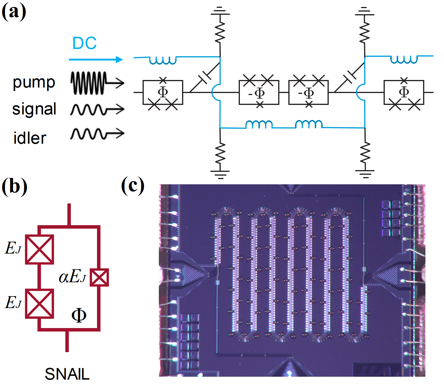
Addressing these issues, our TWPA is a coplanar waveguide (CPW) transmission line where a SNAIL array center conductor simultaneously suppresses the Kerr mixing term and ensures impedance matching, while retaining a sufficient degree of 3WM. In contrast to Ref. Bell and Samolov 2015 where an alternating polarity of SNAIL-like elements suppresses 3WM, our SNAILs (Fig. 1b) have the same dipolar orientation throughout. We realize homogeneous flux biasing for all the 1,632 SNAILs, and negligible off-chip fringing fields, using a magnetic flux bias line placed on chip. The details of the unit cell design that is shown in Fig. 1a are presented in Refs. Vesterinen and Hassel 2020; SI. Resistors keep the flux bias line (depicted in blue in Fig. 1a) grounded at microwave frequencies, thereby acting as L/R lowpass filter and blocking microwave propagation along it. The scheme also contributes towards keeping the two sides of the CPW ground at the same potential. At the same time the resistors prevent leakage of the static current and the formation of parasitic loops of quantized magnetic flux. The resistance value is chosen to be much lower than the reactance of the unit cell shunt capacitor at signal, idler and pump frequencies – 1200, 1200 and 600 times respectively. The resistors thus contribute to the effective loss tangent of the shunt (quantified below), which, however, remains dominated by dielectric loss.
The device (Fig. 1c) was fabricated with a side-wall passivated spacer niobium junction technology detailed in Refs. Grönberg et al. 2017; Simbierowicz et al. 2021. At zero flux bias, the characteristic impedance of the TWPA is far below the optimal value of and the SNAIL non-linearity does not allow for 3WM. Ramping up the bias into the regime near , where is magnetic flux quantum, improves the impedance matching, and the SNAILs exhibit 3WM combined with only weak 4WM. The weakened 4WM contributes favorably to the phase matching of the amplification process and to non-classical state generation.
In a linearly dispersive TWPA the 3WM would strongly and unidirectionally convert pump power into higher harmonics Parameswaran et al. 2002. At angular frequencies higher than the pump (), our TWPA has non-linearly dispersive features primarily from the combination of Josephson plasma resonance and the periodic loading of the CPW with dispersive capacitors Malnou et al. 2021; Vesterinen and Simbierowicz 2021. We control the phase mismatch of the second harmonic generation (SHG) Dixon et al. 2020 in particular. Instead of blocking SHG altogether we allow a weak and cascaded mixing process where the pump accrues a favorable phase shift when converting from to and later back to DeSalvo et al. 1992. The phase shift looks effectively like 4WM and contributes to the compensation of the Kerr effect within the device. The pump frequency is a degree of freedom that allows us explore different levels of SHG and, consequently, to optimize the pump phase shift Vesterinen and Simbierowicz 2021.
Our device provides 15.3 dB of gain over 3 GHz bandwidth with the noise temperature being close to the single-photon quantum limit.
The results on TWPA characterization as a quantum-limited amplifier are presented in Ref. SI.
Although our loss tangent of about isn’t particularly low, 3WM requires a shorter transmission-line length for the same amount of gain as 4WM Zorin 2016.
At our frequency of interest GHz, the unpumped TWPA shows about dB of loss SI, which is to be contrasted against dB and dB extrapolated from Refs. Planat et al. 2020; Bultink et al. 2018.
Such a low loss level is the key feature that allows us to generate entangled quantum states and achieve squeezing.
The experimental scheme for TWPA-based entanglement generation is presented in Fig. 2. The pump signal enters the TWPA at 20 mK temperature through the chain of attenuators and triggers the generation of correlated photons in the frequency bands and generated from vacuum fluctuations Lähteenmäki et al. 2016. Here, is band detuning from frequency , and is the bandwidth that is set manually and can be specified according to the goals. \colorblack In our experiment, GHz, MHz and band separation is varied from 0, the case of minimal mode separation, up to GHz, the maximum mode separation allowed by the bandwidth of our experimental setup. Both and signals exit the TWPA, but only a filtered subband of 4-8 GHz microwaves are amplified using the HEMT and room-temperature amplifiers. \colorblack We record signals using dual-readout configuration, which simultaneously demodulates the bands with two separate IQ mixers Zhong et al. 2013 that are then digitized with a multi-channel Alazar ATS9440 digitizer.
We characterize the entanglement in -mode output quantum state using the covariance formalism. According to the theory of parametric amplifiers, all output states are Gaussian Braunstein and van Loock 2005; Adesso et al. 2014. We verify this assumption by measuring the skewness and kurtosis that prove the Gaussian nature of the signals SI. The state is fully characterized by the covariance matrix of the and voltage quadratures of the propagating microwave modes :
| (2) |
Before the covariance matrix analysis, we calibrate the quadratures in order to be able to compare the variances and covariances to the vacuum noise level, which is crucial for the entanglement verification. We convert quadrature voltages and to the scaled quadratures and in the following way:
| (3) |
with the same transformation applied to . Here, the normalization coefficient is given by
| (4) |
where is measured system gain, , is Planck’s constant, is operating frequency, is the measurement bandwidth and represents internal losses of the TWPA. We rescale the vacuum fluctuations to unity for analysis. Details on system gain calibration and rigorous analysis of quantum modes propagating in the TWPA within distributed gain and loss model are presented in Ref. SI.
Our entanglement analysis employs the Peres-Horodecki criterion of positivity under partial transpose (PPT) Peres 1996; Horodecki 1997 based on symplectic transformation of the covariance matrix Simon 2000.
In a further analysis, we use the logarithmic negativity Vidal and Werner 2002, , that constitutes an upper bound to the distillable entanglement of the state and corresponds to the entanglement cost under PPT preserving operations Audenaert et al. 2003.
\colorblack Here is a minimum symplectic eigenvalue.
Considering the scaled quadratures which correspond to vacuum fluctuations equal to (see Ref. SI), is non zero only if , and it quantifies the quantum information capacity of the entangled state.
We want to emphasize that the low loss level is crucial for the entanglement generation since the internal loss parameter defines the normalization coefficient , which, in turn, affects the minimum symplectic eigenvalue.
black We characterize our results on two-mode () entanglement in terms of logarithmic () negativity. Fig. 3a displays as function of pump power for two different separations of and modes. Mixers used for the downmixing of output signals in the measurement scheme introduce correlations that have classical nature with . Since is an additive quantity, we subtract measured at dBm from the data resulting in at low powers that indicates an uncorrelated ground state of the metamaterial. \colorblack With increasing of pump power, the logarithmic negativity reaches for non-spaced modes at dBm power as shown in the left frame in Fig. 3a. For modes with 2 GHz spacing, we observe similar behaviour with the same maximum logarithmic negativity indicated in the right frame in Fig. 3a. With further increase in pump power, the entanglement disappears since high drive power introduces detrimental higher order couplings and wave-mixing processes Sandbo Chang et al. 2018. \colorblack Similar behaviour has been observed in transmission lines terminated by a SQUID Schneider et al. 2020 and lumped-element JPAs Boutin et al. 2017. In order to prove the nonideality of the state at higher pump powers, we show the decline of purity, calculated for Gaussian states Paris et al. 2003, in Fig. 3a for both spaced and non-spaced modes.
black To demonstrate the broadband entanglement generation we fix the pump frequency and analyse the maximum as a function of separation of modes, see Fig. 3b, and verify the entanglement generation over 2 GHz bandwidth, which is limited by the experimental scheme. In order to generate entanglement over the whole 4 GHz bandwidth, we change the pumping frequency GHz so that the half of the pump was at the center of the measurement band. Such a change in pump frequency degrades impedance matching, resulting in lower logarithmic negativity value, as demonstrated in Fig. 3b. The internal losses and the system gain is measured and calibrated over the whole GHz bandwidth. As can be seen, the logarithmic negativity is nearly constant and starts to decrease only near the bandwidth limit of the experimental setup.
To illustrate the excellent quality of our metamaterial, we demonstrate the generation of vacuum-induced squeezed states. \colorblack For this experiment, we consider two modes with 2 GHz spacing centered at . The parametric amplifier operates in the degenerate mode at this point. Measuring and calibrating and quadratures in the same way as was for two-mode entanglement verification, we introduce and amplitudes that correspond to squeezed and amplified quadratures with respect to the vacuum level. These amplitudes are shown in Fig. 3c as function of the pump power. \colorblack The maximum squeezing of dB is achieved at dBm pump power. Higher powers introduce non-linearities that distort the quantum state and reduce the squeezing, similarly to what occurs for resonant Josephson parametric amplifiers Boutin et al. 2017. \colorblack The same level of squeezing was observed for the single-mode experiment and presented in SI.
In order to quantify our TWPA as a generator of entangled photon flux, we define an entanglement generation rate
| (5) |
that quantifies the production rate of available quantum information.
Here, is the estimation on the photon flux intensity ( ), is the entropy of formation in ebits Bennett et al. 1996 and is the effective bandwidth of the frequency span in which photons are generated from vacuum fluctuations.
The entropy of formation quantifies how many Bell states are needed to prepare the given state using local operations and classical communications, and it is calculated from the minimum symplectic eigenvalue detailed in SI.
\colorblack
We find that our device provides at least Gebits/s (giga entangled bits per second) over 4 GHz, being limited
by the working band of the experimental setup.
Outside of the GHz band, the signal is cut off by circulators, bandpass filters and the bandwidth of the HEMT amplifier, making the entanglement verification impossible at these frequencies.
A similar JPA-based entanglement generation scheme featuring 5 dB of squeezing () and 5 MHz bandwidth Zhong et al. 2013 can provide only 6 Mebits/s – \colorblack three orders of magnitude lower value.
In summary, we have demonstrated a broadband SNAIL Josephson travelling wave parametric amplifier for generation of non-classical states.
\colorblack
Owing to low losses in our 3WM TWPA design, we have been able to generate entangled microwave signals over 4 GHz bandwidth, and with maximum logarithmic negativity with optimized pumping.
For single frequency mode of operation, we reached dB of quantum squeezing.
Higher entanglement generation rate and squeezing can be achieved by further improving the experimental scheme and the TWPA, mainly impedance matching, reducing dielectric losses and dissipation by resistance, and suppressing the Kerr nonlinearity.
Finally, the results presented in this work hold high promise in meeting the challenges of broadband quantum information processing with continuous-variable (CV) states.
\colorblack Indeed, the Kerr effect can be employed in realizing universal quantum gates for CV quantum computing Lloyd and Braunstein 1999; Bartlett and Sanders 2002; Yanagimoto et al. 2020.
In Josephson microwave circuits, Kerr effects are much stronger than in optical systems, and, with the excellent engineering of nonlinearities demonstrated in this work, these proposals may turn out to be realizable.
\colorblack As we demonstrated, the broadband features of the TWPA allow operation over few gigahertz bandwidth, and in combination with the multiple pumping scheme Petrovnin et al. 2021 pave the way towards generation of frequency-spaced multimode entanglement.
Multimode schemes can be employed for various quantum applications, such as CV computing with cluster states Hillmann et al. 2020, secure and robust communications Samsonov et al. 2020, distributed quantum-limited sensing Guo et al. 2019 and search for dark matter Backes et al. 2021.
black During the peer-review process we became aware of the works on squeezing and entanglement generation in TWPAs Esposito et al. 2021b; Qiu et al. 2022.
Acknowledgements.
We thank Alpo Ahonen, Paula Holmlund and Harri Pohjonen for technical assistance and Terra Quantum AG for scientific support. KVP has been funded by the European Union’s Horizon 2020 research and innovation programme under grant agreement no. 862644 (FET-Open project: Quantum readout techniques and technologies, QUARTET). The work at VTT has been funded from the EU Flagship on Quantum Technology Grant No. H2020-FETFLAG-2018-03 Project Nos. 820363 OpenSuperQ and 820505 QMiCS. This project has received funding from the European Union’s Horizon 2020 research and innovation programme under grant agreement no. 824109 (supporting MRP, IL, MW, and AS), no. 862644 (FET-Open project QUARTET), and ERC grant agreement no. 670743 (QuDeT). PJH and VV acknowledge financial support from the Academy of Finland through grants nos. 314448 and 321700, respectively. The work of SHR and PJH was supported by MATINE research grant. GSP and KVP would like to thank Saab for scientific collaboration under a research agreement with Aalto University. This work has been done under the “Finnish Center of Excellence in Quantum Technology QTF” of the Academy of Finland, project nos. 312059, 312294, 312295, 336810, and 312296.Supplemental material for Broadband continuous variable entanglement generation using Kerr-free Josephson metamaterial
I Details of TWPA design and fabrication
The TWPA is realized with VTT’s multilayer superconductive fabrication process Grönberg et al. 2017; Simbierowicz et al. 2021, where the metal and insulator thicknesses vary between 50–200 nm. The fabrication on a high-resistivity silicon wafer begins with the deposition and patterning of a Nb/Al-AlOx/Nb trilayer. We use strips of the trilayer in the SNAILs (110) in Fig. 4. Whenever the subsequent main wiring layer of niobium crosses with a strip, a Josephson junction will form at the cross-over. The ground planes (101) of the coplanar waveguide (CPW) are made of the main wiring layer. The main wiring layer also has dispersive capacitors (open-ended transmission-line spiral resonators Yan et al. 2021; Vesterinen and Simbierowicz 2021 with one side galvanically connected to the CPW center conductor (140) and the other side to the ground) as well as the bottom electrodes of parallel-plate capacitors (120). Next, we uniformly cover the device with atomic layer deposited aluminum oxide insulator. We make contact holes to the insulator at the forthcoming sites of resistors (150), for instance. We cover the insulator with a secondary niobium wiring layer that is used for the magnetic flux bias line (130). The flux line has a meander shape and it repeatedly crosses from one side of the CPW to another. Notably, the flux line also serves as the top electrode of the parallel-plate capacitors (120) Vesterinen and Hassel 2020. The final fabrication step is the deposition and patterning of a normal-metal resistive layer. The resistors (150) connect the flux line on the secondary wiring layer to the ground (101) on the main wiring layer.
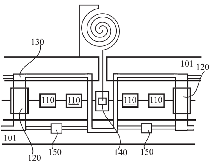
black For details on managing the higher harmonic generation of the pump frequency, we refer to Ref. Vesterinen and Simbierowicz 2021. In brief, we arrange a TWPA dispersion curve that is superlinear at the second harmonic generation (SHG) frequency of the pump. The SHG, which is inherent to 3WM, is phase mismatched and the frequency-doubled microwaves are downconverted with a shifted phase. This refractive effect, which resembles the Kerr effect in 4WM, is well known in the field of non-linear optics DeSalvo et al. 1992. The primary origin of the superlinear dispersion is a stopband near the SHG frequency, induced by the periodic loading of the TWPA with the spiral resonators. The first stopband from the loading occurs when the distance between the spirals corresponds to half a wavelength Malnou et al. 2021. The dispersive effects of the spiral resonator eigenmode and the Josephson plasma frequency are responsible for the phase mismatching of any higher-order non-linear processes above the SHG frequency.
II Control of the wave mixing process in TWPA
To address the non-linearity of the device, we first derive the potential energy of a single SNAIL. We denote the phase of the smaller Josephson junction by , and the total phase of the SNAIL (traversing around the loop) by . With uniform phase drop across the two large junctions, transport current of the SNAIL reads , where is the critical current. Having the voltage-phase relation , one obtains the potential energy of the SNAIL by
| (6) |
with . Assume now that has a minimum at a phase denoted by . We Taylor-expand the potential energy around this point, such that with we have
| (7) |
where . Sitting at the minimum of means that , i.e., the transport current of SNAIL is zero. The coefficients and the Josephson inductance completely determine the behaviour of a SNAIL. However, having an array of SNAILs embedded in a transmission line is more involved and requires careful consideration of the non-linear current conservation. Here, we follow the results presented in Frattini et al. 2018 to address this issue and to estimate the non-linearity of our device, which determines 3WM and 4WM. Consider a simple lumped-element model in which an array of SNAILs are placed in series with a linear inductance and capacitance . Taking as the canonical phase coordinate for the mode, the potential energy of the whole circuit reads
| (8) |
where is the reduced flux quantum. As explained in Frattini et al. 2018, the SNAIL phase is no longer an independent coordinate and needs to be treated as a function of the phase coordinate . This can be achieved by accounting for the non-linear current conservation for the node between the array of SNAILs and the linear inductance:
| (9) |
Taking into account , Taylor expansion of the total potential energy around a minimum determined by yields the coefficients which are related to the corresponding coefficients for a single SNAIL Frattini et al. 2018:
| (10) |
with . 4WM is connected to (Kerr term). According to the expressions above, this term is dependent on in addition to . Therefore, a vanishing does not appear to be sufficient for a Kerr-free situation.
The results of the simple lumped-element model may not be directly applicable to a TWPA as such, but we expect that basically similar observations will hold for coupled-mode equations Zorin 2016; Malnou et al. 2021 describing the waves propagating in the TWPA. All through the TWPA operation, it is important to keep in mind that the effective Kerr coefficient depends not only on but also on a term proportional to . As a consequence, we take both and into account for optimizing the device. The coefficients and are shown in Fig. 5 for various flux and SNAIL asymmetry values. 3WM requires a magnetic flux , where is the magnetic flux quantum. Note that , while .

III Measurement setup
The TWPA was cooled down in a dry dilution refrigerator BlueFors LD400 with 10 mK base temperature. The non-magnetic package for TWPA was made of a copper base, an aluminum lid, and brass connectors with two SMP ports for microwaves and two MMCX ports for the on-chip flux line. The pump signal was generated by ANAPICO APMS12G 4-channel signal generator with -150 dBc/Hz phase noise at 100 kHz. The pump signal was band-pass limited to 8-12 GHz range with Mini-Circuits filters to ensure suppression of signal and was thermalized by a chain of attenuators, -60 dB altogether. The DC signal was generated by Stanford SIM928 Isolated Voltage Source, filtered and routed to flux loops by a superconducting twisted pair cable. \colorblack In order to guide the signals to the output, we use Low Noise Factory circulators 4-12 GHz operating as isolators. The filtered signal in 4-8 GHz range is first amplified by a cooled Low Noise Factory LNC4 8C HEMT amplifier (40 dB of gain and 4 K noise temperature), connected using a BeCu coaxial cable and SMA connectors to a room-temperature amplifier with 44 dB gain. The microwaves are captured with the four-channel 14 bit Alazar ATS9440 digitizer with 125 MS/s rate.
IV TWPA characterization
First, we characterize our device from the perspective of broadband low-noise parametric amplifier in a dry dilution refrigerator at mK. For this purpose, we probe the TWPA with a weak microwave signal (-120 dBm) and apply a pump through the same port, and record the amplified signal. We characterize the amplification performance by measuring the mean gain value normalized against the superconducting transmission line placed in the TWPA’s sample holder over 4–8 GHz frequency range. The best gain performance of the device was observed at a static flux bias of : the mean gain is depicted in Fig. 6a for various pump powers and frequencies. Choosing the best operating point with the pump frequency 9.6 GHz and the pump power -63 dBm (marked with the blue star in Fig. 6a) we evaluate the gain profile depicted in Fig. 6b. The 1-dB compression point indicates the input saturation power of the amplifier is dBm for 20 dB gain.

The noise performance of the TWPA was characterized using the signal to noise ratio improvement method, giving noise relative to system noise temperature Roy et al. 2015. The noise temperature of the device is depicted in Fig. 6b on the bottom. As can be seen from the figure, the noise is close to the single-photon quantum limit over 2 GHz bandwidth centered at 5 GHz, being 350 mK on average (1.45 photons). \colorblack In the case of low pump power, the TWPA features broadband, flat gain profile, see Fig. 6c. We operate the device in such a regime, because the entanglement is generated at low gain.
The quantum efficiency Boutin et al. 2017 is then limited by the noise introduced by TWPA. Efficiency , where is the number of added noise photons, is in the case of high TWPA gain. It is impossible to characterize the added noise when the gain of TWPA is low in the exploited experimental setup.
V Noise calibration
The scheme for the system gain and noise calibration is presented on Fig. 3 in the main text. The calibration was done by measuring the power of the Johnson-Nyquist noise as a function of temperature. During the calibration we vary the noise power generated by components at 20 mK stage by changing the physical temperature of the whole stage. We assume that the output noise of the heated components is fully coupled to the impedance-matched measurement system. The Johnson-Nyquist noise power is given by , where is the Boltzmann constant, is the measurement bandwidth, which is MHz in the experiment, and and are system gain and noise temperature that we aim to estimate. In order to determine the noise power, we measure the temperature-dependent variance of the output voltage, , which was captured at different temperatures using an Anritsu MS2830A Signal Analyzer. The same signal analyzer was used for the entanglement verification. The resulting noise power is given by ; here is 50 .
We calculate the system noise temperature by dividing the noise temperature in the case when TWPA is turned off by the signal-to-noise-ratio improvement using the following formula Roy et al. 2015
| (11) |
where is the signal-to-noise ratio improvement and is TWPA’s gain.
In order to calibrate the and variances for the entanglement verification, we measure the voltage variance when the TWPA is off and extract it from the variance measured in the case TWPA generates photons. Covariances are calculated by normalization per one photon. For the theoretical analysis, the measured voltage quadratures are calibrated and scaled according to the results of prior measurements of the system gain and noise temperature. Using a linear fit of the noise power as function of temperature, we observed that in the case of unpumped TWPA dB (see pump-off case in Fig. 7) and K. We observe that the gain varies with time and the variations are in the range of dB.
VI Loss model: Using the TWPA as an amplifier
To formulate a distributed model for a lossy waveguide with gain, a general mathematical description has been introduced in Ref. Haus 2000. According to this model, each section of the waveguide contains loss per length and gain per length . As the signal propagates along the device, noise will be added, it will get amplified, and will simultaneously decay into the loss channel. Considering the parametric dynamics of a general TWPA, this simple model is addressed further in Ref Houde et al. 2019, which will be also employed in the following.
Consider perfect phase-matching but include distributed loss with identical frequency independent coefficient along the TWPA. The Heisenberg-Langevin equation for the signal mode and idler mode inside the TWPA with the length is then given by [Houde et al. 2019]
| (12) |
where is the group velocity, is the parametric interaction strength, and are noise mode sources. After moving to the frequency domain, one can find a scattering matrix linking the modes at the output of the TWPA, , to those at [Houde et al. 2019]:
| (13) |
where denotes a vertical vector with elements and . Here elements of the scattering matrix are given by
| (14) |
This clearly represents simultaneous gain and loss along the TWPA. In the ideal case that the TPWA is lossless (), one recovers the well-known relation (excluding the global phase):
| (15) |
with . However, when is nonzero the noise sources will be added to the propagating modes and couple due to the parametric interaction, i.e. noise added to the signal contributes to the idler mode and vice versa. For the sake of simplicity, one can adapt a lumped-element picture of Eq. 13 to link the input and output signals of the TWPA. Assuming symmetric loss of signal and idler, one gets
| (16) |
where and describe the gain of the TWPA at signal’s and idler’s frequencies and corresponds to its loss.
The internal losses of TWPA are modeled by the shunt capacitance loss tangent. From the process characterization of the atomic layer aluminum oxide deposition we estimate . The total loss in the waveguide is , where is electrical length of TWPA in radians. The estimated electrical length varies in range rads at that gives dB of internal losses that we use in the calibration. Such a loss value coincides with the one measured in the experiment with the same sample. In that experiment, two microwave switches were used to create two paths: one through the TWPA and one through the resonator placed in the same TWPA’s sample holder. \colorblack Over the whole GHz bandwidth, the average internal loss dB.
VII on-off calibration
In this section we discuss the on-off calibration technique for obtaining the covariance matrix of the output modes of the TWPA based on the covariance matrix of the measured signals at the end of the system [Eichler et al. 2011; Flurin et al. 2015]. We define , where the quadratures are given by and , with the index . We note that by considering these definitions of the quadratures we relate to the real and the imaginary parts of the field’s amplitudes, which we actually measure in the experiment. Assuming zero-mean modes, our aim is to calibrate the covariance matrix with elements at the output of the TWPA since the covariance matrix fully characterizes the Gaussian states. We prove the Gaussian nature of the output signals by measuring the skewness and kurtosis of the signal , where is the standard deviation and . The observed skewness and kurtosis are and respectively, which proves the states are, indeed, Gaussian states.

Suppose that the competition between distributed loss and gain along the TWPA results in an effective power-dependent gain , such that by referring to Eq. 16 one finds . Thus, when the TWPA is pumped the gain can compensate the loss and one has . However, when the pump is off the loss can not be compensated and we get the attenuation . Assuming that the input of the TWPA are vacuum fields , the measured fields in presence of pump () read
| (17) | |||
| (18) |
If the TWPA is not pumped, then the overall gain of the TWPA is described by the attenuation . Considering the noise sources added due to this attenuation, one obtains
| (19) | |||
| (20) |
In further analysis of variances and covariances, we omit all coefficients in normalization except for the gain. Thus, subtracting the covariance matrix of the measured quadratures when the pump is on from the covariance matrix of the measured quadratures when the pump is off yields
| (21) |
where denotes the covariance matrix of the output modes of TWPA, the identity matrix is related to the covariance matrix of the vacuum inputs, and denotes the added noise of the unpumped TWPA due to its loss. Accordingly, one finds
| (22) |
Recalling that , and assuming perfect thermalization for the TWPA’s noise sources in Eqs.(19-20), we obtain
| (23) |
By returning back all normalization coefficients, in addition to multiplying by a factor – to rescale the vacuum fluctuations to (instead of ) – we get the expressions given in Eq. (3) of the main text.
VIII Error analysis
The two main sources of error in the estimation of entanglement strength and squeezing are inaccuracies in the gain of the system and in the internal losses of the TWPA. The system gain is dB and the loss coefficient is dB. This gives an uncertainty of dB for the normalization coefficient . Taking the highest squeezing point we obtain , which is given by the error in normalization coefficients.
IX Rate of Entanglement generation and purity
To quantify the entanglement generation rate of TWPA we introduce . The photon flux intensity is extracted directly from the experiment and is set manually. The entropy of formation according to Refs. Laurat et al. 2005; Flurin et al. 2012 can be calculated from the symplectic eigenvalue using the following relation
| (24) |
where .
The purity of the quantum state is calculated from the covariance matrix : , were is the matrix determinant.
black
X Single-mode squeezing
Besides two-mode entanglement that we characterize with the covariance matrix depicted in Fig. 9a, we demonstrate the generation of single-mode squeezed states. For this experiment, we consider a spanned single mode with 0.5M Hz bandwidth centered at . The parametric amplifier operates in the degenerate mode at this point. These amplitudes are shown in Fig. 9b as function of the pump power. The maximum squeezing of dB is achieved at dBm pump power.
References
- Brecht et al. (2016) T. Brecht, W. Pfaff, C. Wang, Y. Chu, L. Frunzio, M. H. Devoret, and R. J. Schoelkopf, npj Quantum Information 2, 16002 (2016).
- Magnard et al. (2020) P. Magnard, S. Storz, P. Kurpiers, J. Schär, F. Marxer, J. Lütolf, T. Walter, J.-C. Besse, M. Gabureac, K. Reuer, A. Akin, B. Royer, A. Blais, and A. Wallraff, Physical Review Letters 125, 260502 (2020).
- Burkhart et al. (2020) L. D. Burkhart, J. Teoh, Y. Zhang, C. J. Axline, L. Frunzio, M. Devoret, L. Jiang, S. Girvin, and R. Schoelkopf, “Error-detected state transfer and entanglement in a superconducting quantum network,” (2020), arXiv:arXiv 2004.06168 [quant-ph] .
- Lloyd (2008) S. Lloyd, Science 321, 1463 (2008).
- Barzanjeh et al. (2015) S. Barzanjeh, S. Guha, C. Weedbrook, D. Vitali, J. H. Shapiro, and S. Pirandola, Physical Review Letters 114, 080503 (2015).
- Pogorzalek et al. (2019) S. Pogorzalek, K. G. Fedorov, M. Xu, A. Parra-Rodriguez, M. Sanz, M. Fischer, E. Xie, K. Inomata, Y. Nakamura, E. Solano, A. Marx, F. Deppe, and R. Gross, Nature Communications 10, 2604 (2019).
- Candia et al. (2020) R. D. Candia, H. Yiğitler, G. S. Paraoanu, and R. Jäntti, “Two-way covert microwave quantum communication,” (2020), arXiv:arXiv 2004.07192 [quant-ph] .
- Fedorov et al. (2021) K. G. Fedorov, M. Renger, S. Pogorzalek, R. D. Candia, Q. Chen, Y. Nojiri, K. Inomata, Y. Nakamura, M. Partanen, A. Marx, R. Gross, and F. Deppe, “Experimental quantum teleportation of propagating microwaves,” (2021), arXiv:arXiv 2103.04155 [quant-ph] .
- Yurke et al. (1988) B. Yurke, P. G. Kaminsky, R. E. Miller, E. A. Whittaker, A. D. Smith, A. H. Silver, and R. W. Simon, Physical Review Letters 60, 764 (1988).
- Yamamoto et al. (2008) T. Yamamoto, K. Inomata, M. Watanabe, K. Matsuba, T. Miyazaki, W. D. Oliver, Y. Nakamura, and J. S. Tsai, Applied Physical Letters 93, 042510 (2008).
- Hatridge et al. (2011) M. Hatridge, R. Vijay, D. H. Slichter, J. Clarke, and I. Siddiqi, Physical Review B 83, 134501 (2011).
- Lähteenmäki et al. (2012) P. Lähteenmäki, V. Vesterinen, J. Hassel, H. Seppä, and P. Hakonen, Sci. Rep. 2, 276 (2012).
- Mutus et al. (2013) J. Y. Mutus, T. C. White, E. Jeffrey, D. Sank, R. Barends, J. Bochmann, Y. Chen, Z. Chen, B. Chiaro, A. Dunsworth, J. Kelly, A. Megrant, C. Neill, P. J. J. O’Malley, P. Roushan, A. Vainsencher, J. Wenner, I. Siddiqi, R. Vijay, A. N. Cleland, and J. M. Martinis, Applied Physical Letters 103, 122602 (2013).
- Lähteenmäki et al. (2014) P. Lähteenmäki, V. Vesterinen, J. Hassel, G. S. Paraoanu, H. Seppä, and P. Hakonen, Journal of Low Temperature Physics 175, 868 (2014).
- Mutus et al. (2014) J. Y. Mutus, T. C. White, R. Barends, Y. Chen, Z. Chen, B. Chiaro, A. Dunsworth, E. Jeffrey, J. Kelly, A. Megrant, C. Neill, P. J. J. O’Malley, P. Roushan, D. Sank, A. Vainsencher, J. Wenner, K. M. Sundqvist, A. N. Cleland, and J. M. Martinis, Applied Physical Letters 104, 263513 (2014).
- Zhou et al. (2014) X. Zhou, V. Schmitt, P. Bertet, D. Vion, W. Wustmann, V. Shumeiko, and D. Esteve, Phys. Rev. B 89, 214517 (2014).
- Roy et al. (2015) T. Roy, S. Kundu, M. Chand, A. M. Vadiraj, A. Ranadive, N. Nehra, M. P. Patankar, J. Aumentado, A. A. Clerk, and R. Vijay, Applied Physics Letters 107, 262601 (2015).
- Jebari et al. (2018) S. Jebari, F. Blanchet, A. Grimm, D. Hazra, R. Albert, P. Joyez, D. Vion, D. Estève, F. Portier, and M. Hofheinz, Nature Electronics 1, 223 (2018).
- Elo et al. (2019) T. Elo, T. S. Abhilash, M. R. Perelshtein, I. Lilja, E. V. Korostylev, and P. J. Hakonen, Applied Physics Letters 114, 152601 (2019).
- Eichler et al. (2011) C. Eichler, D. Bozyigit, C. Lang, M. Baur, L. Steffen, J. M. Fink, S. Filipp, and A. Wallraff, Physical Review Letters 107, 113601 (2011).
- Wilson et al. (2011) C. M. Wilson, G. Johansson, A. Pourkabirian, M. Simoen, J. R. Johansson, T. Duty, F. Nori, and P. Delsing, Nature 479, 376 (2011).
- Zhong et al. (2013) L. Zhong, E. P. Menzel, R. D. Candia, P. Eder, M. Ihmig, A. Baust, M. Haeberlein, E. Hoffmann, K. Inomata, T. Yamamoto, Y. Nakamura, E. Solano, F. Deppe, A. Marx, and R. Gross, New Journal of Physics 15, 125013 (2013).
- Lähteenmäki et al. (2016) P. Lähteenmäki, G. S. Paraoanu, J. Hassel, and P. J. Hakonen, Nature Communications 7, 12548 (2016).
- Grimsmo and Blais (2017) A. L. Grimsmo and A. Blais, npj Quantum Information 3 (2017), 10.1038/s41534-017-0020-8.
- Schneider et al. (2020) B. H. Schneider, A. Bengtsson, I. M. Svensson, T. Aref, G. Johansson, J. Bylander, and P. Delsing, Phys. Rev. Lett. 124, 140503 (2020).
- Macklin et al. (2015) C. Macklin, K. O'Brien, D. Hover, M. E. Schwartz, V. Bolkhovsky, X. Zhang, W. D. Oliver, and I. Siddiqi, Science 350, 307 (2015).
- White et al. (2015) T. C. White, J. Y. Mutus, I.-C. Hoi, R. Barends, B. Campbell, Y. Chen, Z. Chen, B. Chiaro, A. Dunsworth, E. Jeffrey, J. Kelly, A. Megrant, C. Neill, P. J. J. O'Malley, P. Roushan, D. Sank, A. Vainsencher, J. Wenner, S. Chaudhuri, J. Gao, and J. M. Martinis, Applied Physics Letters 106, 242601 (2015).
- Zorin (2016) A. B. Zorin, Phys. Rev. Applied 6, 034006 (2016).
- Krinner et al. (2019) S. Krinner, S. Storz, P. Kurpiers, P. Magnard, J. Heinsoo, R. Keller, J. Lütolf, C. Eichler, and A. Wallraff, EPJ Quantum Technology 6, 2 (2019).
- Cai et al. (2017) Y. Cai, J. Roslund, G. Ferrini, F. Arzani, X. Xu, C. Fabre, and N. Treps, Nature Communications 8 (2017).
- Esposito et al. (2021a) M. Esposito, A. Ranadive, L. Planat, and N. Roch, Applied Physics Letters 119, 120501 (2021a).
- Vesterinen and Hassel (2020) V. Vesterinen and J. Hassel, “Josephson traveling wave parametric amplifier, WO 2020/152393 A1,” (2020).
- Frattini et al. (2017) N. E. Frattini, U. Vool, S. Shankar, A. Narla, K. M. Sliwa, and M. H. Devoret, Applied Physics Letters 110, 222603 (2017).
- Yurke and Buks (2006) B. Yurke and E. Buks, Journal of Lightwave Technology 24, 5054 (2006).
- Krupko et al. (2018) Y. Krupko, V. D. Nguyen, T. Weißl, É. Dumur, J. Puertas, R. Dassonneville, C. Naud, F. W. J. Hekking, D. M. Basko, O. Buisson, N. Roch, and W. Hasch-Guichard, Physical Review B 98, 094516 (2018).
- Planat et al. (2020) L. Planat, A. Ranadive, R. Dassonneville, J. Puertas Martínez, S. Léger, C. Naud, O. Buisson, W. Hasch-Guichard, D. M. Basko, and N. Roch, Physical Review X 10, 021021 (2020).
- Agrawal (2013) G. Agrawal, Nonlinear Fiber Optics (Elsevier, 2013).
- Malnou et al. (2021) M. Malnou, M. Vissers, J. Wheeler, J. Aumentado, J. Hubmayr, J. Ullom, and J. Gao, PRX Quantum 2, 010302 (2021).
- Ranadive et al. (2021) A. Ranadive, M. Esposito, L. Planat, E. Bonet, C. Naud, O. Buisson, W. Guichard, and N. Roch, “A reversed Kerr traveling wave parametric amplifier,” (2021), arXiv:2101.05815 [quant-ph] .
- Bell and Samolov (2015) M. T. Bell and A. Samolov, Phys. Rev. Applied 4, 024014 (2015).
- Boutin et al. (2017) S. Boutin, D. M. Toyli, A. V. Venkatramani, A. W. Eddins, I. Siddiqi, and A. Blais, Physical Review Applied 8, 054030 (2017).
- Peng et al. (2021) K. Peng, M. Naghiloo, J. Wang, G. D. Cunningham, Y. Ye, and K. P. O’Brien, “Near-ideal quantum efficiency with a Floquet mode traveling wave parametric amplfier,” (2021), arXiv:arXiv 2104.08269 [quant-ph] .
- (43) “See Supplemental Material for the experimental details, loss model, and noise calibration.” .
- Grönberg et al. (2017) L. Grönberg, M. Kiviranta, V. Vesterinen, J. Lehtinen, S. Simbierowicz, J. Luomahaara, M. Prunnila, and J. Hassel, Superconductor Science and Technology 30, 125016 (2017).
- Simbierowicz et al. (2021) S. Simbierowicz, V. Vesterinen, J. Milem, A. Lintunen, M. Oksanen, L. Roschier, L. Grönberg, J. Hassel, D. Gunnarsson, and R. E. Lake, Review of Scientific Instruments 92, 034708 (2021).
- Parameswaran et al. (2002) K. R. Parameswaran, J. R. Kurz, R. V. Roussev, and M. M. Fejer, Optics Letters 27, 43 (2002).
- Vesterinen and Simbierowicz (2021) V. Vesterinen and S. Simbierowicz, “Traveling wave parametric amplifier PCT/FI2021/050283,” (2021).
- Dixon et al. (2020) T. Dixon, J. Dunstan, G. Long, J. Williams, P. Meeson, and C. Shelly, Phys. Rev. Applied 14, 034058 (2020).
- DeSalvo et al. (1992) R. DeSalvo, H. Vanherzeele, D. J. Hagan, M. Sheik-Bahae, G. Stegeman, and E. W. V. Stryland, Optics Letters 17, 28 (1992).
- Bultink et al. (2018) C. C. Bultink, B. Tarasinski, N. Haandbæk, S. Poletto, N. Haider, D. J. Michalak, A. Bruno, and L. DiCarlo, Applied Physics Letters 112, 092601 (2018).
- Braunstein and van Loock (2005) S. L. Braunstein and P. van Loock, Reviews of Modern Physics 77, 513 (2005).
- Adesso et al. (2014) G. Adesso, S. Ragy, and A. R. Lee, Open Systems & Information Dynamics 21, 1440001 (2014).
- Peres (1996) A. Peres, Physical Review Letters 77, 1413 (1996).
- Horodecki (1997) P. Horodecki, Physics Letters A 232, 333 (1997).
- Simon (2000) R. Simon, Physical Review Letters 84, 2726 (2000).
- Vidal and Werner (2002) G. Vidal and R. F. Werner, Physical Review A 65, 032314 (2002).
- Audenaert et al. (2003) K. Audenaert, M. B. Plenio, and J. Eisert, Physical Review Letters 90, 027901 (2003).
- Sandbo Chang et al. (2018) C. W. Sandbo Chang, M. Simoen, J. Aumentado, C. Sabín, P. Forn-Díaz, A. M. Vadiraj, F. Quijandría, G. Johansson, I. Fuentes, and C. M. Wilson, Physical Review Applied 10, 044019 (2018).
- Paris et al. (2003) M. G. A. Paris, F. Illuminati, A. Serafini, and S. De Siena, Physical Review A 68, 012314 (2003).
- Bennett et al. (1996) C. H. Bennett, D. P. DiVincenzo, J. A. Smolin, and W. K. Wootters, Physical Review A 54, 3824 (1996).
- Lloyd and Braunstein (1999) S. Lloyd and S. L. Braunstein, Physical Review Letters 82, 1784 (1999).
- Bartlett and Sanders (2002) S. D. Bartlett and B. C. Sanders, Physical Review A 65, 042304 (2002).
- Yanagimoto et al. (2020) R. Yanagimoto, T. Onodera, E. Ng, L. G. Wright, P. L. McMahon, and H. Mabuchi, Physical Review Letters 124, 240503 (2020).
- Petrovnin et al. (2021) K. V. Petrovnin, M. R. Perelshtein, I. Lilja, T. Korkalainen, V. Vesterinen, G. S. Paraoanu, and P. J. Hakonen, (to be published) (2021).
- Hillmann et al. (2020) T. Hillmann, F. Quijandría, G. Johansson, A. Ferraro, S. Gasparinetti, and G. Ferrini, Physical Review Letters 125, 160501 (2020).
- Samsonov et al. (2020) E. Samsonov, R. Goncharov, A. Gaidash, A. Kozubov, V. Egorov, and A. Gleim, Scientific Reports 10, 10034 (2020).
- Guo et al. (2019) X. Guo, C. R. Breum, J. Borregaard, S. Izumi, M. V. Larsen, T. Gehring, M. Christandl, J. S. Neergaard-Nielsen, and U. L. Andersen, Nature Physics 16, 281 (2019).
- Backes et al. (2021) K. M. Backes, D. A. Palken, S. A. Kenany, B. M. Brubaker, S. B. Cahn, A. Droster, G. C. Hilton, S. Ghosh, H. Jackson, S. K. Lamoreaux, A. F. Leder, K. W. Lehnert, S. M. Lewis, M. Malnou, R. H. Maruyama, N. M. Rapidis, M. Simanovskaia, S. Singh, D. H. Speller, I. Urdinaran, L. R. Vale, E. C. van Assendelft, K. van Bibber, and H. Wang, Nature 590, 238 (2021).
- Esposito et al. (2021b) M. Esposito, A. Ranadive, L. Planat, S. Leger, D. Fraudet, V. Jouanny, O. Buisson, W. Guichard, C. Naud, J. Aumentado, F. Lecocq, and N. Roch, “Observation of two-mode squeezing in a traveling wave parametric amplifier,” (2021b), arXiv:2111.03696 [quant-ph] .
- Qiu et al. (2022) J. Y. Qiu, A. Grimsmo, K. Peng, B. Kannan, B. Lienhard, Y. Sung, P. Krantz, V. Bolkhovsky, G. Calusine, D. Kim, A. Melville, B. M. Niedzielski, J. Yoder, M. E. Schwartz, T. P. Orlando, I. Siddiqi, S. Gustavsson, K. P. O’Brien, and W. D. Oliver, “Broadband squeezed microwaves and amplification with a Josephson traveling-wave parametric amplifier,” (2022), arXiv:2201.11261 [quant-ph] .
- Yan et al. (2021) C. Yan, J. Hassel, V. Vesterinen, J. Zhang, J. Ikonen, L. Grönberg, J. Goetz, and M. Möttönen, “Low-noise on-chip coherent microwave source,” (2021), arXiv:arXiv 2103.07617 [quant-ph] .
- Frattini et al. (2018) N. E. Frattini, V. V. Sivak, A. Lingenfelter, S. Shankar, and M. H. Devoret, Phys. Rev. Applied 10, 054020 (2018).
- Haus (2000) H. A. Haus, Electromagnetic Noise and Quantum Optical Measurements (Springer Berlin Heidelberg, 2000).
- Houde et al. (2019) M. Houde, L. Govia, and A. Clerk, Phys. Rev. Applied 12, 034054 (2019).
- Flurin et al. (2015) E. Flurin, N. Roch, J. D. Pillet, F. Mallet, and B. Huard, Phys. Rev. Lett. 114, 090503 (2015).
- Laurat et al. (2005) J. Laurat, T. Coudreau, G. Keller, N. Treps, and C. Fabre, Physical Review A 71, 022313 (2005).
- Flurin et al. (2012) E. Flurin, N. Roch, F. Mallet, M. H. Devoret, and B. Huard, Physical Review Letters 109, 183901 (2012).