Why the first magic-angle is different from others in twisted graphene bilayers: interlayer currents, kinetic and confinement energy and wavefunction localization Preprint: APS/123-QED
Abstract
The chiral Hamiltonian for twisted graphene bilayers is analyzed in terms of its squared Hamiltonian which removes the particle-hole symmetry and thus one bipartite lattice, allowing to write the Hamiltonian in terms of a matrix. This brings to the front the three main physical actors of twisted systems: kinetic energy, confinement potential and an interlayer interaction operator which is divided in two parts: a non-Abelian interlayer operator and an operator which contains an interaction energy between layers. Here, each of these components is analyzed as a function of the angle of rotation, as well as in terms of the wave-function localization properties. In particular, it is proved that the non-Abelian operator represents interlayer currents between each layer triangular sublattices, i.e., a second-neighbor interlayer current between bipartite sublattices. A crossover is seen between such contributions and thus the first magic angle is different from other higher order magic angles. Such angles are determined by a balance between the negative energy contribution from interlayer currents and the positive contributions from the kinetic and confinement energies. A perturbative analysis performed around the first magic angle allows to explore analytically the details of such energy balance.
I Introduction
Twisted bilayer graphene (TBG) exhibits unconventional superconducting phases and Mott insulating states Cao et al. 2018. Such discovery was made by working upon previous theoretical efforts which suggested a path to increase many body interactions Bistritzer and MacDonald 2011; dos Santos et al. 2007; San-Jose et al. 2012. In particular, MacDonald et. al. Bistritzer and MacDonald 2011 found that at certain twisting angles, TBG presents flat-bands where the Fermi-velocity goes to zero. Several works confirmed the existence of such flat bands at certain “magic angles” where the electron-electron interactions are maximized Cao et al. 2018; Kerelsky et al. 2019.
Yet there are still many open questions concerning this problem Cyprian et al. 2021; Xueheng et al. 2021; Pietro et al. 2020; Nguyen et al. 2021; A. et al. 2017; Ledwith et al. 2021a, even in the one-particle operator limit. For example, the wave function of TBG has been found to be reminiscent of a quantum Hall wave function in a torus and this opens new analogies to the physics of Landau levels Uri et al. 2020; Hejazi et al. 2019; Popov and Milekhin 2020; Sheffer and Stern 2021, the Hofstadter butterfly Crosse et al. 2020; Moon and Koshino 2013; Oka and Koshino 2021; Benlakhouy et al. 2021 or the fractional quantum Hall effect Dean et al. 2013. There is also an interesting connection to topological phases, Moiré edge states and Weyl semimetals Tsim et al. 2020; Fujimoto and Koshino 2021; Pantaleón et al. 2021; Lin et al. 2021; Wu et al. 2020; Fu et al. 2020.
Also, as the Moiré pattern generates a high electron density localization, interest in making quantum dots with TBG has been steadily increasing M. et al. 2020; Wang et al. 2021a. Other interesting applications have been found Fidrysiak et al. 2018; Jian et al. 2020; Kangjun et al. 2019; Rodriguez-Vega et al. 2020; Yankowitz et al. 2019; Hejazi et al. 2019; Christophe De Beule and Recher 2020; Xu and Balents 2018; Rosendo López et al. 2020; Singh and Benjamin 2021, as well as optical/electrical signatures Herrera and Naumis 2021; Phong et al. 2019.
The mobility/stability of electrons is influenced by the triangular geometry of the TBG Koshino et al. 2018; Guo et al. 2018; Bagchi et al. 2020; Park et al. 2019. Previous papers have studied nematicity andd Cao et al. 2021; Liu et al. 2021; Kimura et al. 2021, phonons/plasmons Cyprian et al. 2021; Koshino and Son 2019, disorder effects Sainz-Cruz et al. 2021; Ochoa and Fernandes 2021; Wilson et al. 2020 and other important related properties San-Jose et al. 2012; Goodwin et al. 2019a; Cea et al. 2020; Solís-Fernández and Hiroki 2021; Vincent et al. 2021; Phong et al. 2021; Li et al. 2021; Sánchez-Ochoa et al. 2021. However, a direct analytic connection with the presence of superconducting phases at magic angles has not yet been achieved completely. As expected, the interacting behavior of electrons in the Hubbard model is important to characterize the electronic correlations and its fermionic behavior Koshino et al. 2018; Hofmann et al. 2021; Vafek and Kang 2021; Vahedi et al. 2021; Sboychakov et al. 2019.
An important mechanism in the properties of Moiré systems is the superlattice relaxation Koshino and Nam 2020; Carr et al. 2019; Angeli et al. 2018. This is specially important near AA stacking points, where interlayer hopping tends to be reduced.
Theoretically, when the hopping that couples layers in AA regions is tuned off the system becomes exactly chiral symmetric Tarnopolsky et al. 2019. This model shows a recurrence at magic angles and reduces the problem to a more analytically manipulable Hamiltonian operator. For this reason among others, the chiral Hamiltonian reduces the complexity of the continuum model and captures all the important symmetries and physics of TBG Tarnopolsky et al. 2019. The mathematical properties and structure of the wavefunction have been rigorously studied in several works Popov and Milekhin 2020; Zou et al. 2018; Yafei et al. 2021; Ledwith et al. 2021b; Chichinadze et al. 2021. As one can imagine the graphene layer as two triangular sublattices each one with an equal magnetic flux but with opposite sign, therefore, TBG graphene consists of coupled magnetic fluxes with opposite sign between layers Khalaf et al. 2020; Sboychakov et al. 2020; Ledwith et al. 2021. This produces a strong skyrmion behavior in which electrons form vortexes, reflected in the presence of strong electron-electron correlation on specific locations across the Moiré superlattice Goodwin et al. 2019b.
To further understand the physics behind the problem, in a previous work we considered the squared Hamiltonian (SH) of the chiral model Gerardo et al. 2021. This represents a renormalization of the TBG that removes one of the bipartites triangular sublattices for each graphene layer Naumis 2007; Barrios-Vargas and Naumis 2011; Barrios-Vargas and Naumis 2013; Gerardo et al. 2021. In general, the physics of the SH is the same as that of the original Hamiltonian but the renormalizated operator allows to see properties that in the original model were hidden or difficult to identify. For example, it reveals three physical driving mechanisms: kinetic energy, an effective confinement potential and a non-Abelian gauge field leading to magnetic fields. It also allows to write the Hamiltonian as a simple operator and then use Pauli matrices in which topological properties are more evident. But more importantly, it gives a direct physical interpretation of magic angles in terms of the wave-function geometrical frustration, i.e., we showed that such renormalization folds the spectrum around zero energy and thus zero-mode states correspond to antibonding ground states in a triangular lattice Gerardo et al. 2021. As is well known, antibonding states in triangular lattices are frustrated as the wave-function can not achieve a phase difference of between sites. This cost energy and usually push states into highly degenerate spectral regions and thus to a nearby depletion of states seen as gaps or pseudogaps Naumis et al. 1994; Naumis et al. 2002; Barrios-Vargas and Naumis 2011; Barrios-Vargas and Naumis 2013. In Ref. (Gerardo et al. 2021) we showed that magic angles occur whenever the interlayer frustration is exactly zero. Then at magic angles a highly degenerated state is formed and separated by a gap from the rest of the spectrum. Such effect is achieved by a very precise fine tuning of the wave function Fourier coefficients akin to the Hall effect. Notice that although previous works showed some peculiarities about frustration properties Hridis et al. 2019; Nguyen et al. 2021; T. et al. 2019, it was not clear why such states were at the middle of the band. The same happens with the analytical form of zero-modes, which were identified as reminiscent of a Hall effect ground state without a clear explanation of why the lowest Landau level was found at the middle of the spectrum and not at its bottom end Tarnopolsky et al. 2019; Ledwith et al. 2021.
Yet, several spectral analysis hinted that the first magic angle is differently from others Tarnopolsky et al. 2019; Ledwith et al. 2021; Jie et al. 2021. For example, numerically it was found that the spectrum of the TBG chiral model shows a remarkable recurrence rule for the magic angles Tarnopolsky et al. 2019, however, the first angle does not follows it and the reason is not known. As we will see here, their wave functions charge density and phases are remarkably different from others. Thus, it would be very useful to understand the reason of why such behaviors differ from other magic angles. For this reason, here we present such an study. Also, this work allows to discern how the physical mechanisms scale between each other as the twist angle is changed.
The layout of this work is the following. In section II we present the model to be studied and the identification of the main physical contributions to the problem. Then in section III we study the zero modes wave functions and its localization. In section IV, we study the expectation values of each energy contribution and discuss the interlayer current contribution, in section V we show why the first magic angle is different from others. Finally, the conclusions are given in the last section.
II Squared Twisted Bilayer Graphene chiral Hamiltonian
The chiral Hamiltonian of twisted bilayer graphene is a variant of the original Bistritzer-MacDonald Hamiltonian in which the tunneling is set to zero Ledwith et al. 2021. We use as basis the wave vectors where the index represents each graphene layer and and are the Wannier orbitals on each inequivalent site of the graphene’s unit cell. The chiral Hamiltonian is given Tarnopolsky et al. 2019; Eslam et al. 2019; Patrick et al. 2020,
| (1) |
where the zero-mode operator is defined as,
| (2) |
and,
| (3) |
with , . The potential is,
| (4) |
where the phase factor and the Moiré lattice vectors are given by , , , the Moiré modulation vector is with is the magnitude of the Dirac wave vector and is the lattice constant of monolayer graphene, see Fig. 1. The physics of this model is captured by the parameter , defined as where is the interlayer coupling of stacking AB/BA with value meV and is the Fermi velocity with value . Notice that the Hamiltonian Eq. (1) was originally written in Ref. Tarnopolsky et al. 2019 using units where , , thus the operators and are dimensionless. This allows to treat the system with a fixed geometry for any twist angle as in this units , , . The twist angle thus only enters in the dimensionless parameter .

By a renormalization procedure which consists in taking the square of , we found that Gerardo et al. 2021,
| (5) |
The squared norm of the potential is an effective confinement potential,
| (6) |
where are the Moiré Brillouin zone (mBZ) vectors and . In Fig. 2, we plot in real space, with the Wigner-Seitz indicated. This effective potential has an hexagonal structure where the point in the stacking lays in the maximum point of this potential and the minimums lay in the and stacking points. The off-diagonal terms in are,
| (7) |
and,
| (8) |
where with and . This is an essential point as eigenvalues must be reals (notice that ). We also define the following operator which contains all the non-diagonal contributions,
| (9) |
Also, is a set of unitary vectors perpendicular to the set ,
| (10) |
The importance of such renormalization is that now we can see the three main ingredients of the problem: i) the kinetic contribution via the term (which leads to frustration), ii) a confinement potential and, iii) the interlayer interaction .

An important feature that we will further analyze is that is made from two terms, and therefore is convenient to define separately the quantities,
| (11) |
and
| (12) |
where the dimensionless projected momentum operators are , as the dimensionless momentum operator is . See how Eq. (11) is akin to a Lorentz force term.
Let us also comment some useful symmetries of as they play important roles in the presence of flat-bands You and Vishwanath 2019; Zou et al. 2018. For our purposes, the most important symmetry is the exact intravalley inversion symmetry Jie et al. 2021, that produce flat-bands and the chirality. The exact intravalley inversion symmetry operator is Jie et al. 2021,
| (13) |
where the and operators are acting on the sublattice and layer degrees of freedom respectively and given by two different sets of Pauli matrices Jie et al. 2021. Using such definition we have,
| (14) |
Our renormalized Hamiltonian also preserves this symmetry as,
| (15) |
For the chiral TBG, intravalley inversion follows from the group symmetry, where represents time reversal and is the cyclic group of order . The action of is that complex conjugates and exchanges the two sublattices. In the following section we will further analyze the interplay between the different terms in and the role played by the symmetries.
III Wave functions: localization properties
In this section we discuss the localization properties of the zero-modes wave functions for different angles to see if there are differences between the first and higher-order magic angles. We start with the Schrödinger equation . Considering only the first spinor component of , the explicit form of the zero-modes wave function is Tarnopolsky et al. 2019,
| (16) |
where and represents the Fourier coefficients of each spinor component representing layers and , respectively, and where are the Moiré Brillouin zone vectors and .
For the flat-bands, it has been proved that Tarnopolsky et al. 2019,
| (17) |
where . is given in terms of Jacobi theta functions Tarnopolsky et al. 2019, or alternatively as a Weierstrass sigma function Jie et al. 2021. Therefore, the electronic density for layer is with .
As the analytic form of is known, our interest here is focused on the study of which corresponds to the ground state of at all angles.
In Fig. 3 we present the resulting plots in real space at the first magic angles and for each layer component, obtained by plugging Eq. (16) into to obtain recurrence relations for the ’s and ’s. As expected, present the rotational symmetry.

Several features are worth noticing, i) the first magic angle is different from the others as the amplitude is centered at the stacking points, ii) it tracks the form of the confining potential, iii) at other angles the density is confined at somewhat similar locations but never at points as in the first one.
At the first magic angle one can use perturbation theory Tarnopolsky et al. 2019 to obtain the density (see the Appendix),
| (18) |
where and the other component,
| (19) |
This solution allows to understand the coincidence between Fig. 2 and the first angle in Fig. 3 as basically, the is just proportional the confinement potential.
In Fig.4 the real and imaginary parts of the wave function for each layer are shown and the Wigner-Seitz cell is indicated as well. The wave functions present vortices but the most important feature to be seen in Fig.4 is the lack of vortices for the component 1 at the first magic angle, as well as for the component 2 in the AA stacking point. Such features are in agreement with the perturbative solution for such angle. Although at this moment there are not published figures of the phases to compare with, intralayer currents present vortices Jie et al. 2021. However, the vortices of such currents do not coincide with the wavefunction vortices, a feature to be expected since they are made from a sum of different points wavefunctions. Theoretically it has been suggested that the pairing of the wavefunction vortices are a special signature of the TBG from where superconductivity arises Khalaf et al. 2020. Here, what is most important for us is the very different behavior of the phases and density associated with the first magic angle when compared with others.

To further highlight such differences, in Fig. 5 we plot the amplitude of the Fourier coefficients and for each layer. Again we see that the first magic angle is remarkably different from the others, as its main Fourier components contributions are around the origin. However, for the second, third and fourth magic angle there is a hole at . This hole appears at . Also, when , both layers have nearly the same spectral behavior of the Fourier components.

The Fourier components of in general form complex patterns. However, as seen in Fig. 5, at the points most of the coefficients , are negligible and the Fourier spectrum consists of six localized peaks forming hexagonal patterns for high values of . Moreover, we find that at the -th magic angle , the main contributions of the coefficients are given by . Notably, has been associated with a Landau-level index Jie et al. 2021.
As the wave functions in reciprocal space change but keep a well localized peak, this means that the localization behavior is far from trivial. To test numerically such observation, here we measure the localization by using a inverse participation ratio Thouless 1974; Wegner 1980; Bell and Dean 1970 (IPR) ,
| (20) |
where is the index of the top and bottom component of the spinor.

In Fig 6 we present the IPR for each layer. Analyzing the behavior of the IPR for the top and bottom component. In the limit , the IPR reproduces the expected solution . In the interval the wavefunction becomes less delocalized while becomes more localized. When increases, there is an oscillation in the and . Magic angles occur at inflexion points or at minimas and there is a tendency to increase the overall localization in both layers when .
Suprisingly, the IPR for magic angles is the same for all states in the flat band as, except at the poles,
| (21) |
even though is a complex meromorphic function. The reason of such relation comes from the normalization of any state corresponding to the flat-band as we must have,
| (22) |
where denotes integration over the mBZ. Then we observe that the wavefunction for is also normalized as well, from where it follows that in order to be consistent we must have (notice that the poles of are cancelled out by the zeros of ). We have verified numerically that such condition is true.
To summarize the results of this section, again there are clear signatures in the wave functions that the first magic angle is different from others.
IV Expectation Values and Interlayer currents
To understand the contribution of each physical driving term in the squared Hamiltonian and why the first magic angle is different, we next calculate the expected value of each corresponding operator in . From the eigenvalue equation , where , and using Eq. (5),
| (23) |
where the expected values for a given layer are,
| (24) |
| (25) |
and , with,
| (26) |
and
| (27) |
Notice that and are not exactly properly defined expected values as involve the bracket of two different wave function components and thus they can be or not complex values. However, the total contribution expected value of the whole off-diagonal terms is real. The total kinetic energy is while the total confinement energy is,
| (28) |
where the last bound is obtained using the wave function normalization.
To understand how depends on the two contributions coming from the off-diagonal terms in , we will define the space-dependent expected value of the gradient terms in Eq. (5) as,
| (29) |
which come from the non-diagonal, gradient part, of ,
| (30) |
Therefore,
| (31) |
By adding its complex conjugate we obtain that,
| (32) |
where we defined the interlayer currents as,
| (33) |
and
| (34) |
Such definitions are unusual as involve two different wavefunctions from each layer and only one sublattice. Thus, this requires some comments and thoughts. In recent papers, J. Wang et. al Jie et al. 2021; Wang et al. 2021b; Wang and Liu 2021 proposed a somewhat analogous definition for a second-neighbor intralayer current, i.e., these authors defined,
| (35) |
where .
Such definition is required as the usual current is obtained from which turns out to be zero in the ground state. Therefore, they defined a current in one of the bipartite lattice as can be seen by performing a tight-binding calculation of the intralayer orbital current. Here we do not need to appeal to such recourse as already the square Hamiltonian initially renormalized the hexagonal lattice in a triangular lattice and therefore the second neighborhood interaction is implicit in the renormalization procedure. In Ref. Jie et al. 2021 it was argued that if is discretized in a tight-binding Hamiltonian, we have that where and creates and anhiliates respectively electrons in site .
In a similar way, if in Eq. (31) we discretize the spinor components gradient we have that and the other current component as . Therefore, this leads to the interpretation of an interlayer current.
Let us now integrate over the primitive cell in order to get the expected value of the current. By noting that it follows that,
| (36) |
where and . Therefore, is just the sum of the Fourier components of the current at the points , and . In a similar way, the space-dependent expected value of the second ingredient of is,
| (37) |
where , and we define the operator,
| (38) |
V Expectation values and currents at different points
In this section we study all contributions defined in the previous section as a function of the twist at representative points in space. One is the point which reveals how magic angles arise and the other is the point, which is the ground state for all . Fig. 7 shows such behavior as obtained from the numerical simulation, i.e, the top of the band goes to zero at the magic angles while is the ground state. The point, chosen at random in the mBZ, lies inside such interval.
V.1 Revealing the magic angles: point expected values
From Fig. 7 we see that can be used to reveal the magic angles as always gives the highest energy of the first band. For a flat band to exist, the energy must be zero.

For the point it is very illustrative to use perturbation theory in the limit . As shown in the Appendix, up to linear order in we have that,
| (39) |
| (40) |
It follows that,
| (41) |
In Fig. 8 we present a comparison between these expected values and the numerical results showing a good agreement for , , as . For , the agreement is not so good as this requires higher order perturbation terms. The previous approximation allows to make a crude estimate of the first magic angle as,
| (42) |
Therefore, , a value below . Higher order terms in the expansion are needed to increase the accuracy, but yet the main principle behind a magic angle is already present in this simple approach. Further confirmation is provided in Fig. 9 where we show numerically how magic angles arise whenever the curve intersects .

Then we conclude that in going from to , the confinement potential starts to contribute and reaches the kinetic energy at the magic angle. The off-diagonal operators always diminish the energy. As expected, the first magic angle is thus produced when the sum of the kinetic plus confinement energies are equal in magnitude to the expected values of the off-diagonal operators. The particularity here is that for we have .

The numerical results in Fig. 9 show how the same principle applies for other magic angles as goes to zero. However, as seen in Fig. 10, for the current term dominates over , and in fact, can be neglected as we will discuss in the following subsection. Notice also the jumps associated to each , possibly related with Landau levels. The other particularity is that as , thus in Fig. 9 one can not distinguish one from the other in such scale.

V.2 Ground state: point
The point is a ground state for any . Let us do some general considerations about it. As and , it follows that for , we have that and . Fig. 11 numerically confirms these results. Other interesting features are seen. The first is already clear from Eq. (23); for the ground state and due to symmetry we obtain,
| (43) |
and,
| (44) |
The derivation that follows is made by considering a symmetrized basis Gerardo et al. 2021. In this case, there is no way to distinguish the up and low layers except for a relative phase, it follows that we must have and . As the general flat-band solutions are given by Jie et al. 2021,
| (45) |
where is a Bloch wave function and is the quantum Hall wavefunction of the lowest Landau level, we replace such wave function into the expressions for and to show that,
| (46) |
This is a reminiscent condition of the intravalley symmetry of Eq. (1). Therefore, for the total kinetic energy and total confinement energy we have that,
| (47) |
Using the bound for the confinement energy, we find that is bounded by,
| (48) |

Fig. 11 further confirms Eq. (47) and Eq. (48). Also, in Fig. 12 we compare the numerical results with the perturbative approach up to second order in as detailed in the Appendix. The agreement is excellent and allows to: i) further confirm analytically Eq. (47) in the limit and, ii) test the validity of the numerical approach.

From the previous results is clear that will always diminish with to compensate the increased value of the confinment and kinetic terms. However, such interlayer interaction depends on two terms as in the point. This requires a further analysis.

In Fig. 13 we present the interlayer current for in real space. The vectors directions represent polar angle defined by the real and imaginary parts of or . For the first magic angle , has more density in the AA stacking point while has more current around the BA/AB stacking points. On the other hand, for the second magic angle , and have three points of high intensity inside the Wigner-Seitz cell. Also,it is interesting to note that in the AA/AB stacking points there is a vortex behavior as those seen in Fig. 4.
Using the spinor symmetry (45) and integrating over the primitive cell, it follows that,
| (49) |
where means a convolution, is the Fourier transform of .
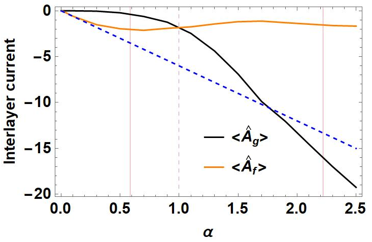
In Fig. 14, we show the evolution of Eq. (36) and (49). Clearly, for the first magic angle, and have similar magnitudes but become radically separated after the first magic angle, i.e., . Therefore, the terms is only relevant for making the first magic angle different from others as in the point. The reason for such change is easy to see as is bounded by the norm of the wavefunctions and thus,
| (50) |
a fact further corroborated by using Eq. (45) to find its explicit form,
| (51) |
Meanwhile, is proportional to the gradient which is not bounded by .

Further confirmation is obtained by looking at the perturbative solution (see Appendix). In particular while and . Then . This ratio goes from zero at to at .
V.3 Comparison between different points
The previous analysis was made for . In Fig. 15 and Fig. 16 we extend the analysis for other flat-band states at magic angles. Fig. 15 presents and in reciprocal space. For the first magic angle , the term is maximal where is minimal, both have similar magnitude range. On the other hand, for higher magic angles, the reciprocal space structure of and preserve the same behavior, however, has a substantially increased magnitude than . If , . As a consequence, the analysis made for can be safely extended for all flat-band states.
Therefore, is only relevant for making the first magic angle different from others. As said before, is limited by while is proportional to the wave function gradient. Moreover, as the IPR baseline increases as seen in Fig. 6, gradients grow. However, in principle the overlap between the gradient in one layer and the other layer wave function can diminish. As is proportional to , to test the gradient effects, in Fig. 16 we plot . This indicates that currents due to gradients are the responsible of the effect. This behavior is also reflected in Fig. 5, as in the crossover the Fourier coefficients develop a ”hole” around . Notice in Fig. 16 that the magic angles fall inside ”basins”. Such effect is specially prominent for non high symmetry points as the point, a fact that will be discussed in a forth coming publication.

Summarizing, the term is an energy associated with interlayer current leakage between bipartite sublattices, i.e., at second neighbors. Meanwhile, is a weighted average energy associated with overlaps between layers. The interlayer current magnitude grows as the rotation angle goes to zero, a fact due to the ever increasing spatial gradients of the electron wave function.
VI Conclusions
In this work we presented a theoretical and numerical analysis of the chiral TBG Hamiltonian using a renormalized Hamiltonian that removes the particle-hole symmetry allowing to identify the main physical elements of the problem and leading to a simple matrix operator. Then we studied the electron localization in the TBG. We found numerically that the first magic angle is different from others as the ground state wave function basically tracks the shape of the confinement potential. We calculated the localization using the inverse participation ratio where magic angles are revealed. Interestingly, we proved that all states in the flat band for magic angles have the same participation ratio. We also evaluated the contributions from the kinetic energy, confinement energy and inter-layer interaction for the and points. These contributions were found using perturbation theory and numerically. A good agreement between both was found. Our analysis shows that the point reveals how magic angle arises.
In particular we found that the first magic angle in the point occurs when : 1) the confinement and kinetic energies are the same, 2) the off-diagonal operator is the sum of kinetic and confinement energy, 3) the intralayer current is bigger that the off-diagonal interaction energy term although not negligible. At other magic angles, the balance is dictated only by the kinetic, confinement and interlayer current. Therefore, interlayer currents are the main responsible for bands to shrink.
In other works, the magic angle effects have been associated with the effects of a space dependent magnetic field Patrick et al. 2020; Jie et al. 2021. Our results are in agreement with this idea as the interlayer current can also be interpreted as a Lorentz force too. However, allowed us to identify the source of this field: the current between the graphene’s underlying triangular sublattices.
It is temping to try to identify our results with some geometrical feature of the twist angle. However, contains both the geometry and the scale of the energy interaction. Here we found that both are needed in order to make the confinement reach the kinetic energy and produce a strong interlayer current. For very big angles, confinement is just too weak. This is confirmed by the IPR which at the first magic angle has the same value on each layer. We can also argue that the remarkable rule in the recurrence of happens in the limit when , as for higher magic angles the nodal structure of the lowest Landau level does not depend significantly on the Moiré unit cell flux.
VII acknowledgment
We thank UNAM-DGAPA project IN102620 and CONACyT project 1564464. Thanks CONACyT schoolarship for providing critical support during the COVID emergency.
VIII Appendix: Perturbative analysis of expected values
VIII.1 at the point
Consider the limit for the point. The corresponding wave function was found in Ref. Tarnopolsky et al. 2019,
| (52) |
and , where is a counterclockwise rotation on angle with and , the minus sign is used for odd magic angles. The normalization factor is,
| (53) |
In this case, it is instructive to analyze first how operates on the wave function. Consider for example one of the differential equations resulting form Eq. (5),
| (54) |
where the square of energy is also expanded in powers of , i.e., . Next we use the relationship between wave functions on different layers,
| (55) |
If we collect terms up to order using Eq. (52), two equations are obtained. The zero order equation is,
| (56) |
and at order ,
| (57) |
From Eq. (56) we recover as,
| (58) |
and using we prove that Eq. (56) is indeed true whenever , in agreement with Ref. Tarnopolsky et al. 2019.
Now consider Eq. (57). As we did for the order zero component, is easy to show that,
| (59) |
Next we compute using the two operators and . Using the definition for and we have,
| (60) |
and the sum term is then divided in terms with and ,
| (61) |
Using that and defining a new index ,
| (62) |
From the definition of we finally obtain,
| (63) |
Let us know consider the operator action. We have,
| (64) |
from where,
| (65) |
Next we use that where is the sign of the permutation of the indices and , for even and for odd. Each pair permutation is obtained from the usual cyclic order , so for example, while . Again we use ,
| (66) |
where . Finally,
| (67) |
Then we collect all the previous results inside Eq. (57) using to confirm that the wave vector is an eigenvector of ,
| (68) |
i.e., comparing terms, we get .
The previous analysis confirms that the solutions of are also eigenfunctions of . Now we find the expected values of each operator and for the corresponding differential equation. We start with the kinetic energy in the first layer,
| (69) |
Using that Eq. (56), (59) and that and are ortogonal due to symmetry, the contribution of order is zero, from where . Now taking into account the contribution from the equation that results from the second row of Eq. (5), we have . Then, up to order ,
| (70) |
In a similar way, as and are ortogonal,
| (71) |
Finally, the other operators are,
| (72) |
while,
| (73) |
It follows that,
| (74) |
In Fig. 8 we compare the previous results with the numerical simulation obtaining a good agreement as .
VIII.2 at the point
Here we consider a perturbative solution of Eq. (75) for in the point as was found in Ref. Tarnopolsky et al. 2019,
| (75) |
Considering only terms up to order we get:
| (76) |
These functions must be normalized before calculating the expected values. The normalization factor is,
| (77) |
With these expresions for and we obtain
| (78) |
and
| (79) |
for . Therefore, taking into account an extra and factor from the operator definition, we have,
| (80) |
This result is in agreement with the predicted bound found in Eq. (50). Consider in the same limit the other operator. We have that,
| (81) |
and the terms containg give the same result. This confirms Eq. (46), i.e., . By collecting terms we finally obtain that,
| (82) |
Next we find the expected values of the kinetic and confining potential operators to confirm the theoretical and numerical analysis. Using that,
| (83) |
| (84) |
and,
| (85) |
| (86) |
It follows that,
| (87) |
and for the kinetic energy term,
| (88) |
By expanding the denominators we arrive to the final perturbative expectation values,
| (89) |
| (90) |
and,
| (91) |
| (92) |
References
- Cao et al. [2018] Y. Cao, V. Fatemi, S. Fang, K. Watanabe, T. Taniguchi, E. Kaxiras, and P. Jarillo-Herrero, Nature 556, 43 (2018).
- Bistritzer and MacDonald [2011] R. Bistritzer and A. H. MacDonald, Proceedings of the National Academy of Sciences 108, 12233 (2011).
- dos Santos et al. [2007] J. M. B. L. dos Santos, N. M. R. Peres, and A. H. C. Neto, Phys. Rev. Lett. 99, 256802 (2007).
- San-Jose et al. [2012] P. San-Jose, J. González, and F. Guinea, Phys. Rev. Lett. 108, 216802 (2012).
- Kerelsky et al. [2019] A. Kerelsky, L. McGilly, and D. e. a. Kennes, Nature 572, 95 (2019).
- Cyprian et al. [2021] Cyprian, Lewandowski, Debanjan, Chowdhury, and J. Ruhman, Phys. Rev. B 103, 235401 (2021).
- Xueheng et al. [2021] Xueheng, Kuang, Zhen, Zhan, and S. Yuan, Phys. Rev. B 103, 115431 (2021).
- Pietro et al. [2020] Pietro, Novelli, I. Torre, Frank, H., L., Koppens, Fabio, Taddei, and M. Polini, Phys. Rev. B 102, 125403 (2020).
- Nguyen et al. [2021] V. H. Nguyen, D. Paszko, M. Lamparski, B. Van Troeye, V. Meunier, and J. C. Charlier, arXiv e-prints , arXiv:2102.05376 (2021).
- A. et al. [2017] L. A., Gonzalez-Arraga, J.L., F. Lado, Guinea, Pablo, and San-Jose, Phys. Rev. Lett. 119, 107201 (2017).
- Ledwith et al. [2021a] P. J. Ledwith, E. Khalaf, and A. Vishwanath, arXiv e-prints , arXiv:2105.08858 (2021a), arXiv:2105.08858 [cond-mat.str-el] .
- Uri et al. [2020] A. Uri, S. Grover, Y. Cao, J. Â. A. Crosse, K. Bagani, D. Rodan-Legrain, Y. Myasoedov, K. Watanabe, T. Taniguchi, P. Moon, M. Koshino, P. Jarillo-Herrero, and E. Zeldov, Nature (London) 581, 47 (2020).
- Hejazi et al. [2019] K. Hejazi, C. Liu, and L. Balents, Phys. Rev. B 100, 035115 (2019).
- Popov and Milekhin [2020] F. K. Popov and A. Milekhin, arXiv e-prints , arXiv:2010.02915 (2020), arXiv:2010.02915v1 [cond-mat.mes-hall] .
- Sheffer and Stern [2021] Y. Sheffer and A. Stern, Phys. Rev. B 104, L121405 (2021), arXiv:2106.10650 [cond-mat.str-el] .
- Crosse et al. [2020] J. A. Crosse, N. Nakatsuji, M. Koshino, and P. Moon, Phys. Rev. B 102, 035421 (2020).
- Moon and Koshino [2013] P. Moon and M. Koshino, Phys. Rev. B 88, 241412 (2013).
- Oka and Koshino [2021] H. Oka and M. Koshino, Phys. Rev. B 104, 035306 (2021).
- Benlakhouy et al. [2021] N. Benlakhouy, A. Jellal, H. Bahlouli, and M. Vogl, arXiv e-prints , arXiv:2112.13614 (2021), arXiv:2112.13614 [cond-mat.mes-hall] .
- Dean et al. [2013] C. R. Dean, L. Wang, P. Maher, C. Forsythe, F. Ghahari, Y. Gao, J. Katoch, M. Ishigami, P. Moon, M. Koshino, T. Taniguchi, K. Watanabe, K. L. Shepard, J. Hone, and P. Kim, Nature 497, 598–602 (2013).
- Tsim et al. [2020] B. Tsim, N. N. T. Nam, and M. Koshino, Phys. Rev. B 101, 125409 (2020).
- Fujimoto and Koshino [2021] M. Fujimoto and M. Koshino, Phys. Rev. B 103, 155410 (2021).
- Pantaleón et al. [2021] P. A. Pantaleón, T. Low, and F. Guinea, Phys. Rev. B 103, 205403 (2021).
- Lin et al. [2021] X. Lin, B.-B. Chen, W. Li, Z. Y. Meng, and T. Shi, arXiv e-prints , arXiv:2110.00200 (2021), arXiv:2110.00200 [cond-mat.str-el] .
- Wu et al. [2020] F. Wu, R.-X. Zhang, and S. Das Sarma, Phys. Rev. Research 2, 022010 (2020).
- Fu et al. [2020] Y. Fu, E. J. König, J. H. Wilson, Y.-Z. Chou, and J. H. Pixley, npj Quantum Materials 5, 71 (2020), arXiv:1809.04604 [cond-mat.str-el] .
- M. et al. [2020] M., Mirzakhani, F., M., Peeters, , M., and Zarenia, Phys. Rev. B 101, 075413 (2020).
- Wang et al. [2021a] Y. Wang, G. Yu, M. Rösner, M. I. Katsnelson, H.-Q. Lin, and S. Yuan, arXiv e-prints , arXiv:2110.01323 (2021a), arXiv:2110.01323 [cond-mat.mes-hall] .
- Fidrysiak et al. [2018] M. Fidrysiak, M. Zegrodnik, and J. Spałek, Phys. Rev. B 98, 085436 (2018).
- Jian et al. [2020] Jian, Kang, Oskar, and Vafek, Phys. Rev. Lett. 102, 035161 (2020).
- Kangjun et al. [2019] Kangjun, Seo, Valeri, N., Kotov, Bruno, and Uchoa, Phys. Rev. Lett. 122, 246402 (2019).
- Rodriguez-Vega et al. [2020] M. Rodriguez-Vega, M. Vogl, and G. A. Fiete, Phys. Rev. Research 2, 033494 (2020).
- Yankowitz et al. [2019] M. Yankowitz, S. Chen, H. Polshyn, Y. Zhang, K. Watanabe, T. Taniguchi, D. Graf, A. F. Young, and C. R. Dean, Science 363, 1059 (2019).
- Christophe De Beule and Recher [2020] y. M.-H. L. Christophe De Beule, Peter G. Silvestrov and P. Recher, arXiv e-prints , arXiv:1912.03191 (2020), arXiv:1912.03191v2 [cond-mat.mes-hall] .
- Xu and Balents [2018] C. Xu and L. Balents, Phys. Rev. Lett. 121, 087001 (2018).
- Rosendo López et al. [2020] M. Rosendo López, F. Peñaranda, J. Christensen, and P. San-Jose, Phys. Rev. Lett. 125, 214301 (2020).
- Singh and Benjamin [2021] A. Singh and C. Benjamin, Phys. Rev. B 104, 125445 (2021).
- Herrera and Naumis [2021] S. A. Herrera and G. G. Naumis, Phys. Rev. B 104, 115424 (2021).
- Phong et al. [2019] V. o. T. Phong, Z. Addison, S. Ahn, H. Min, R. Agarwal, and E. J. Mele, Phys. Rev. Lett. 123, 236403 (2019).
- Koshino et al. [2018] M. Koshino, N. F. Q. Yuan, T. Koretsune, M. Ochi, K. Kuroki, and L. Fu, Phys. Rev. X 8, 031087 (2018).
- Guo et al. [2018] H. Guo, X. Zhu, S. Feng, and R. T. Scalettar, Phys. Rev. B 97, 235453 (2018).
- Bagchi et al. [2020] S. Bagchi, H. T. Johnson, and H. B. Chew, Phys. Rev. B 101, 054109 (2020).
- Park et al. [2019] M. J. Park, H. S. Kim, and S. Lee, Phys. Rev. B 99, 245401 (2019).
- andd Cao et al. [2021] Y. andd Cao, Daniel, Rodan-Legrain, Jeong, Min, Park, Noah, F. Q., Yuan, K. Watanabe, Takashi, Taniguchi, Rafael, M., Fernandes, Liang, Fu, Pablo, and Jarillo-Herrero, Science Advances 372, 264 (2021).
- Liu et al. [2021] S. Liu, E. Khalaf, J. Y. Lee, and A. Vishwanath, Phys. Rev. Research 3, 013033 (2021).
- Kimura et al. [2021] K. Kimura, M. Sigrist, and N. Kawakami, arXiv e-prints , arXiv:2110.01308 (2021), arXiv:2110.01308 [cond-mat.str-el] .
- Koshino and Son [2019] M. Koshino and Y.-W. Son, Phys. Rev. B 100, 075416 (2019).
- Sainz-Cruz et al. [2021] H. Sainz-Cruz, T. Cea, P. A. Pantaleón, and F. Guinea, Phys. Rev. B 104, 075144 (2021).
- Ochoa and Fernandes [2021] H. Ochoa and R. M. Fernandes, Degradation of phonons in disordered moiré superlattices (2021), arXiv:2108.10342 [cond-mat.mes-hall] .
- Wilson et al. [2020] J. H. Wilson, Y. Fu, S. Das Sarma, and J. H. Pixley, Phys. Rev. Research 2, 023325 (2020).
- Goodwin et al. [2019a] Z. A. H. Goodwin, F. Corsetti, A. A. Mostofi, and J. Lischner, Phys. Rev. B 100, 121106 (2019a).
- Cea et al. [2020] T. Cea, P. A. Pantaleón, and F. Guinea, Phys. Rev. B 102, 155136 (2020).
- Solís-Fernández and Hiroki [2021] P. Solís-Fernández and A. Hiroki, arXiv e-prints , arXiv:2110.04115 (2021), arXiv:2110.04115 [cond-mat.mtrl-sci] .
- Vincent et al. [2021] T. Vincent, K. Kawahara, V. Antonov, H. Ago, and O. Kazakova, arXiv e-prints , arXiv:2107.08919 (2021), arXiv:2107.08919 [cond-mat.mtrl-sci] .
- Phong et al. [2021] V. T. Phong, P. A. Pantaleón, T. Cea, and F. Guinea, Phys. Rev. B 104, L121116 (2021), arXiv:2106.15573 [cond-mat.mes-hall] .
- Li et al. [2021] Y. Li, A. Eaton, H. A. Fertig, and B. Seradjeh, arXiv e-prints , arXiv:2107.10687 (2021), arXiv:2107.10687 [cond-mat.mes-hall] .
- Sánchez-Ochoa et al. [2021] F. Sánchez-Ochoa, A. R. Botello-Méndez, and C. Noguez, Phys. Rev. B 104, 075430 (2021).
- Hofmann et al. [2021] J. S. Hofmann, E. Khalaf, A. Vishwanath, E. Berg, and J. Y. Lee, arXiv e-prints , arXiv:2105.12112 (2021), arXiv:2105.12112 [cond-mat.str-el] .
- Vafek and Kang [2021] O. Vafek and J. Kang, Phys. Rev. B 104, 075143 (2021), arXiv:2106.05670 [cond-mat.str-el] .
- Vahedi et al. [2021] J. Vahedi, R. Peters, A. Missaoui, A. Honecker, and G. Trambly de Laissardière, arXiv e-prints , arXiv:2104.10694 (2021), arXiv:2104.10694 [cond-mat.str-el] .
- Sboychakov et al. [2019] A. O. Sboychakov, A. V. Rozhkov, A. L. Rakhmanov, and F. Nori, Phys. Rev. B 100, 045111 (2019).
- Koshino and Nam [2020] M. Koshino and N. N. T. Nam, Phys. Rev. B 101, 195425 (2020).
- Carr et al. [2019] S. Carr, S. Fang, Z. Zhu, and E. Kaxiras, Phys. Rev. Research 1, 013001 (2019).
- Angeli et al. [2018] M. Angeli, D. Mandelli, A. Valli, A. Amaricci, M. Capone, E. Tosatti, and M. Fabrizio, Phys. Rev. B 98, 235137 (2018).
- Tarnopolsky et al. [2019] G. Tarnopolsky, A. J. Kruchkov, and A. Vishwanath, Phys. Rev. Lett. 122, 106405 (2019).
- Zou et al. [2018] L. Zou, H. C. Po, A. Vishwanath, and T. Senthil, Phys. Rev. B 98, 10.1103/PhysRevB.98.085435 (2018).
- Yafei et al. [2021] Yafei, Ren, Qiang, Gao, A., H. MacDonald, , Qian, and Niu, Phys. Rev. Lett. 126, 016404 (2021).
- Ledwith et al. [2021b] P. J. Ledwith, A. Vishwanath, and E. Khalaf, arXiv e-prints , arXiv:2109.11514 (2021b), arXiv:2109.11514 [cond-mat.str-el] .
- Chichinadze et al. [2021] D. V. Chichinadze, L. Classen, Y. Wang, and A. V. Chubukov, arXiv e-prints , arXiv:2108.05334 (2021), arXiv:2108.05334 [cond-mat.str-el] .
- Khalaf et al. [2020] E. Khalaf, S. Chatterjee, N. Bultinck, M. P. Zaletel, and A. Vishwanath, arXiv e-prints , arXiv:2004.00638 (2020), arXiv:2004.00638 [cond-mat.str-el] .
- Sboychakov et al. [2020] A. O. Sboychakov, A. V. Rozhkov, A. L. Rakhmanov, and F. Nori, Phys. Rev. B 102, 155142 (2020).
- Ledwith et al. [2021] P. J. Ledwith, E. Khalaf, and A. Vishwanath, Annals of Physics , 168646 (2021).
- Goodwin et al. [2019b] Z. A. H. Goodwin, F. Corsetti, A. A. Mostofi, and J. Lischner, Phys. Rev. B 100, 235424 (2019b).
- Gerardo et al. [2021] Gerardo, G. Naumis, L. A., Navarro-Labastida, Enrique, Aguilar-Méndez, Abdiel, and Espinosa-Champo, Phys. Rev. B 103, 245418 (2021).
- Naumis [2007] G. G. Naumis, Phys. Rev. B 76, 153403 (2007).
- Barrios-Vargas and Naumis [2011] J. E. Barrios-Vargas and G. G. Naumis, Journal of Physics: Condensed Matter 23, 375501 (2011).
- Barrios-Vargas and Naumis [2013] J. Barrios-Vargas and G. G. Naumis, Solid State Communications 162, 23 (2013).
- Naumis et al. [1994] G. G. Naumis, R. A. Barrio, and C. Wang, Phys. Rev. B 50, 9834 (1994).
- Naumis et al. [2002] G. G. Naumis, C. Wang, and R. A. Barrio, Phys. Rev. B 65, 134203 (2002).
- Hridis et al. [2019] Hridis, K. Pal, Stephen, Spitz, Markus, and Kindermann, Phys. Rev. Lett. 123, 186402 (2019).
- T. et al. [2019] T., M., R., Wolf, J., L., Lado, G., Blatter, , O., and Zilberberg, Phys. Rev. Lett. 123, 096802 (2019).
- Jie et al. [2021] Jie, Wang, Yunqin, Zheng, Andrew, J., Millis, and J. Cano, Phys. Rev. Research 3, 023155 (2021).
- Eslam et al. [2019] Eslam, Khalaf, A. J., Kruchkov, Grigory, Tarnopolsky, Ashvin, and Vishwanath, Phys. Rev. B 100, 085109 (2019).
- Patrick et al. [2020] Patrick, J., Ledwith, Grigory, Tarnopolsky, Eslam, Khalaf, Ashvin, and Vishwanath, Phys. Rev. Research 2, 023237 (2020).
- You and Vishwanath [2019] Y.-Z. You and A. Vishwanath, npj Quantum Materials 4, 16 (2019).
- Thouless [1974] D. Thouless, Physics Reports 13, 93 (1974).
- Wegner [1980] F. J. Wegner, Zeitschrift für Physik B Condensed Matter 36, 209 (1980).
- Bell and Dean [1970] R. J. Bell and P. Dean, Discuss. Faraday Soc. 50, 55 (1970).
- Wang et al. [2021b] J. Wang, J. Cano, A. J. Millis, Z. Liu, and B. Yang, arXiv e-prints , arXiv:2105.07491 (2021b), arXiv:2105.07491 [cond-mat.mes-hall] .
- Wang and Liu [2021] J. Wang and Z. Liu, arXiv e-prints , arXiv:2109.10325 (2021), arXiv:2109.10325 [cond-mat.mes-hall] .