Variable Selection and Missing Data Imputation in Categorical Genomic Data Analysis by integrated Ridge Regression and Random Forest
Abstract
Genomic data arising from a genome-wide association study (GWAS) are often not only of large-scale, but also incomplete. A specific form of their incompleteness is missing values with non-ignorable missingness mechanism. The intrinsic complications of genomic data present significant challenges in developing an unbiased and informative procedure of phenotype-genotype association analysis by a statistical variable selection approach. In this paper we develop a coherent procedure of categorical phenotype-genotype association analysis, in the presence of missing values with non-ignorable missingness mechanism in GWAS data, by integrating the state-of-the-art methods of random forest for variable selection, weighted ridge regression with EM algorithm for missing data imputation, and linear statistical hypothesis testing for determining the missingness mechanism. Two simulated GWAS are used to validate the performance of the proposed procedure. The procedure is then applied to analyze a real data set from breast cancer GWAS.
1 Introduction
A single-nucleotide polymorphism (SNP) refers to a genetic variant at a locus on a chromosome pair which should be present in at least of a population. It is known that a genetic disease or phenotype may be intricately related to a small set of SNPs. A number of genome-wide association studies (GWAS) have been carried out in genomics for identifying such SNPs that are associated with the risk of a phenotype. However, genomics data collected for GWAS often contain missing values on SNPs all over the place due to limitations of DNA sequencing techniques. Ignoring the missing data in GWAS is likely to give biased or even misleading information to the downstream work, especially when the missing data are not missing at random (NMAR) and the missingness mechanism is not ignorable.
In cases of the missing data being missing (completely) at random (MAR or MCAR), relatively simple methods are available for accommodating them for GWAS. For example, a so-called single imputation method is often used where each missing value of a SNP for an individual can be replaced by this SNP’s most frequent value observed in the population stratum this individual belongs to. See e.g. chapter 7 of Foulkes (2009) and R package pan of Grund et al. (2016) for details.
In cases of handling NMAR missing values of SNPs in GWAS, one needs a statistical model to describe the randomness involved in the SNPs having missing values, and another model to characterize the missingness mechanism. Baker & Laird (1988) used a log-linear regression model for analyzing categorical variables involving non-ignorable missing values. Joint probability distribution of the covariates having missing values is modelled by the product of a sequence of one-dimensional conditional distributions in Lipsitz & Ibrahim (1996). This approach is extended by Ibrahim et al. (1999) to model the missingness mechanism as well as the covariates having missing values. It was further extended by Stubbendick & Ibrahim (2003) to handle the missing values and missingness mechanism in random effect models.
Since the SNPs having missing values in a GWAS may be large in number and widespread across the population with the missingness mechanism unclear, one should resort to statistical models to describe the joint probability distributions of the missing values and the missingness mechanism, from which multiple rather than single imputations can be generated to substitute the missing SNPs values involved in each individual.
Several computational tools, such as fastPhase Scheet & Stephens (2006) and Impute Marchini et al. (2007), have been developed to impute SNP missing values based on a statistical model for the SNPs, where the linkage disequilibrium (LD) between SNPs is also taken into account. The Emlasso developed by Sabbe et al. (2013) does the imputation implicitly based on the EM algorithm Dempster et al. (1977) and a generalized location model (GLoMo) Olkin & Tate (1961). However, these imputation methods overlook the missingness mechanism that may be non-ignorable. In this paper, we propose a new method of multiple imputations through integrating a current such method with multiple logistic models for the missingness mechanism. Ridge regression Hoerl & Kennard (1981) will be used to fit the resultant model if the number of covariates involved is large.
Since we use multiple logistic models to describe the SNPs missingness mechanism, we are able to apply a well-developed linear hypothesis testing method to test whether or not the missingness of a SNP variable depends significantly on any available SNP variables or the phenotype variable. Therefore, a conclusion on whether or not the missingness mechanism of a SNP variable is ignorable can be drawn based on statistical evidence. This is an advantage of modelling the missingness mechanism by a parametric statistical model.
The set of SNPs significantly associated with the phenotype could be inferred from applying a variable selection procedure to the joint log-likelihood function combining the phenotype-genotype conditional association probabilities, the joint probability of the SNPs having missing values, and the conditional probability of the missingness mechanism. But this is computationally infeasible because the dimension of the selection space is proportional to the number of SNPs under investigation, leading to combinatorial explosion in computing complexity. In this paper, we propose to use a supervised machine learning approach, to be briefed below, for SNPs selection after we substitute the generated multiple imputations for the missing values. This approach is shown to be computationally feasible.
The phenotype-SNPs association can be delineated by some machine learning models, upon which SNPs variable selection can be computationally feasibly performed. An examples is lasso Tibshirani (1996) when the phenotype-SNPs association is represented by a logistic regression model. Another example is elastic-net Zou & Hastie (2005) which is effective for variable selection when the SNPs in the logistic model are not only of high-dimensional but also highly correlative.
Ensemble classification and regression trees (CART) model gives a more flexible description of the phenotype-SNPs association, and is likely to result in better prediction performance. Feasible variable selection also can be performed on an ensemble CART model. For example, in random forest (RF) model proposed by Breiman (2001) one can compute a variable importance (VIMP) measure for each SNP variable, and rank all SNPs in the model by the VIMP measure. Accordingly, the most important SNPs associated with the phenotype are selected to be those top ranked.
The main ideas of RF are two-folded: (i) Bootstrapping the data sample, by which a tree is constructed for each bootstrap sample of the data; (ii) Sub-sampling the predictors (mostly referred to the SNPs here-and-after) so that a randomly selected subset of the SNPs are used to decide the best split at each node-splitting stage. The out of bag (OOB) errors are then aggregated across all trees in an RF to give a total prediction error of the model, from which a VIMP measure for each SNP is derived for variable selection. More details on the VIMP measure are given in section 2.2.
Chen & Ishwaran (2012) reviews the applications of RF for genomic data analysis and variable selection, where three influential RF techniques for cases of high-dimensional and highly correlative SNPs are discussed in detail. The first one is the gene-shaving random forest (GSRF) of Jiang et al. (2004). GSRF performs iterations of RF and backward variable elimination/selection by: (i) Re-computing the retained SNPs’ VIMP values after each SNPs backward elimination; (ii) Computing the total prediction errors based on both the OOB samples and independent test samples. The second one is the gene selection random forest (GeneSrF) of Díaz-Uriarte & De Andres (2006), which enhances the computing efficiency over GSRF by: (i) computing the VIMP values in the first iteration of RF only; (ii) the prediction errors being computed on only the OOB samples. The third one is from Calle et al. (2011) which replaces the mis-classification error used in the previous two techniques with the ROC curve’s AUC as the prediction accuracy measure. We choose to use the GeneSrF technique for its performance regarding computing efficiency.
In this paper, we develop a coherent procedure of categorical phenotype-SNPs association analysis, in the presence of missing values with non-ignorable missingness mechanism in GWAS data, by integrating the state-of-the-art methods reviewed in this section, namely, random forest for variable selection, weighted ridge regression with EM algorithm for missing data imputation, and linear statistical hypothesis testing for determining the missingness mechanism. The paper is organized as follows. We first develop the proposed method in Section 2. In Section 3, we conduct two simulation studies to assess the method’s performance and illustrate its use in practice. Then we apply the proposed method to analyze a real data set from the Australian breast cancer and mammographic density GWAS in Section 4. Finally, Section 5 discusses the improvements and future work extending the proposed method.
2 Method
The method we are to develop is motivated by the need of addressing the missing value problem in the Australian Breast Cancer Family Study (ABCFS) Dite et al. (2003) and the Australian Mammographic Density Twins and Sisters Study (AMDTSS)Odefrey et al. (2010). A specific data subset from ABCFS and AMDTSS contains observations of 207 SNPs on a specific gene pathway, suspected to be susceptible to breast cancer, for 596 individuals comprising 354 breast cancer patients and 242 matched controls. Each SNP variable for an individual in the data takes a value from 0, 1 and 2, representing the number of the minor alleles at the individual’s SNP loci. The response variable in the data is binary indicating whether an individual has breast cancer or not. The data contain 1,724 missing values out of 123,372 SNP observations. The proportion of missing values is about 1.4% but they distribute across all SNPs and individuals widely and irregularly. Specifically, 157 SNPs have missing values with each SNP being missing in between 1 to 32 individuals; 513 individuals have missing SNP values with each individual having 1 to 9 such missing SNP values; 50 SNPs have no missing values on all 596 individuals; and 83 individuals have no missing values on all 207 SNPs.
It is clear that we first need to develop a statistical model capable of characterizing those data as seen above, which may involve non-ignorable missing values and large number of highly correlative SNPs, in order to effectively analyze them and find out which predictor variables are significantly associated with the response variable. Section 2.1 below will present this model together with its fitting procedure and our proposed missing value multiple imputation method. In section 2.2 we develop an RF induced variable selection procedure for identifying the most important predictors to the response variable. The variable selection and missing value multiple imputation are executed in iteration until convergence. The corresponding computational method is also presented in section 2.2. Then we present a linear hypothesis testing procedure in section 2.3 to infer the missingness mechanism.
2.1 Model and notations
Let , and denote a binary response variable having no missing values, a predictor vector having no observed missing values, and a predictor vector having observed missing values, respectively. In the context of GWAS data analysis, indicates the presence, and indicates the absence of a phenotype (e.g. breast cancer). In the same context, and refer to the SNPs in the data. Recall that a SNP variable is coded as the number of minor allele at a locus, thus takes 3 possible values 0, 1 and 2, representing the three states of the alleles pair: homozygous recessive, heterozygous, and homozygous dominant. Gauderman et al. (2007) used an alternative way to code a SNP to express it as either dominant or recessive.
We choose to code each SNP by two dummy variables and . Thus, assume that is a vector of dummy variables plus constant 1 for SNPs (denoted as ) having no missing values, and is a vector of dummy variables for SNPs (denoted as ) having missing values. Then for each , , , and . The same equivalences hold for each as well.
Denote , and as the th observation of , and , respectively, with individual . The observations of can be reasonably assumed to be independently and identically distributed in a case-control study. If denote as the real value of for individual . Then we have , , and . The same equivalences hold for each as well. Since has missing values, let be the missingness indicator vector of the SNPs; and be the th observation of , i.e. if the value of individual is missing, and otherwise, ; . For convenience of presentation, we write , , and in the sequel.
Given and , follows a Bernoulli distribution with probability of phenotype which satisfies a logistic regression model
| (1) |
where , and is a unknown parameter vector specifying the effects of the SNPs on the phenotype which is to be estimated from the data. By (1) the joint conditional probability of given is
| (2) |
Since each contains missing value(s), a joint probability distribution is needed to model . Using the approach of Lipsitz & Ibrahim (1996), the joint probability of equals the product of a sequence of conditional trinomial probabilities. Denote
| (3) |
which are conditional probabilities with , respectively. Here is the vector of the first elements of (Note ). Writing with , we can naturally propose a trinomial logistic regression model for these conditional probabilities
| (4) |
where is the first columns of , and with is a unknown parameter vector giving the associations of and with and is to be estimated from the data. Denote with . By (3) and (4) the joint probability function of equals
| (5) |
And by (5) the joint probability function of given is
| (6) |
Since the missing values in the data may be non-ignorable, a joint probability distribution is needed to model the missingness mechanism. Namely, the joint conditional probability distribution of each missingness indicator vector given is needed, where each follows a Bernoulli distribution with probability with and . By Ibrahim et al. (1999) this joint conditional probability function can be expressed as the product of a sequence of univariate conditional probability functions, as given below
| (7) |
where is the first elements of , and is an unknown parameter vector specifying the parametric structure of . It can be seen that and . We propose to model the missingness probabilities by a set of logistic regression equations as given below
| (8) |
for , where gives the effect of on the missingness mechanism of and is the first columns of . By (7) and (8) the joint conditional probability of given is
| (9) | |||||
Equations (1), (4) and (8) together with(2), (6) and (9) provide a system of logistic regression models for analyzing the complete data , from which the phenotype-SNPs association can be inferred. To perform such inference we first need to estimate the unknown parameter vector by method of maximum likelihood. From (2), (6) and (9) it is easy to see the join log-likelihood function of given the complete data is
| (10) | |||||
where is the complete data log-likelihood for individual . However, the maximum likelihood estimator (MLE) of cannot be obtained by maximizing , because contains missing values. On the other hand, it is not feasible to compute the MLE of through maximizing the observed data log-likelihood , with the summation being taken over all possible values of the missing part of , due to the involved mathematical intractability and the fact that the ’s in may be high-dimensional and in the state of linkage disequilibrium (LD).
To overcome this difficulty we propose to use EM algorithm Dempster et al. (1977) and the ridge regression idea Hoerl & Kennard (1981) to compute , a penalized maximum likelihood estimator (PMLE) of , i.e.
| (11) |
where is the -norm, and are tuning parameters that may be optimized by cross-validation or BIC to be detailed later in the paper. To reduce the computing complexity we may set . For given value of , PMLE is computed by the following Ridge-EM algorithm.
Algorithm 1
Computing PMLE by ridge-expectation-maximization (Ridge-EM):
-
Set a plausible initial estimate for .
-
Repeat for until convergence of computation:
-
E-step Compute
(12) where the first term is the expectation of with respect to the conditional distribution of given the observed data. Here and are the observed and the missing part of , respectively. Note that the parameter value is in the conditional distribution of .
-
M-step Find by solving .
-
-
The PMLE . By the method of Louis (1982), we estimate by
(13)
It is not difficult to show that the estimate obtained from the Ridge-EM algorithm is indeed the PMLE under general regularity conditions. However, a full implementation of the Ridge-EM algorithm until convergence would be computationally very intensive and actually not necessary, when many redundant predictor variables are still not removed from the logistic regression system (1, 4, 8) in use. We suggest to fully implement the Ridge-EM algorithm only at the final stage when all insignificant predictors are eliminated from the system. Before this final stage, we propose a missing value multiple imputation method to simplify the Ridge-EM algorithm.
For in the E-step it can be shown that
| (14) | |||||
where and are the observed and missing parts of , respectively. Thus, subject to a permutation of . Here means the summation over all possible values that can take, where denotes the number of SNP variables with their values for individual being missing (clearly ). Each term in (14) is the conditional probability , i.e.
| (15) |
If we regard the possible values that each can take as the imputations for , which together with the observed data constitute the complete data (for individual ), then in (14) can be seen as a penalized weighted log-likelihood function of for the complete data. Therefore, computed from the M-step is just the maximum penalized weighted log-likelihood estimate (MPWLE) that can be computed from fitting the logistic regression system (1, 4, 8) with the complete data.
Clearly, depends on and , tuning of which for optimal model estimation may be computationally intensive. Therefore, we set and tune only in Ridge-EM. This should have little impact on optimal model estimation because the predictors involved in (1, 4, 8) are of the similar scale and magnitude. Tuning for best value could be carried out by cross-validation, which in fact is difficult to implement in practice. This is because the missingness pattern of the predictors in a training sample may be different from that in a validation sample in cross-validation. A consequence of such variation in the missingness pattern is that fitting the model system (1, 4, 8) is likely to encounter singularity, in that some missingness indicator variable has no variation across the training sample although varies across all samples. Hence, modification is needed to avoid such singularity if one still chooses to use cross-validation. For example, generalized cross-validation (GCV) of Craven & Wahba (1978) may be used. In this paper we propose to use a BIC Schwarz (1978) based approach for tuning . Knowing that with being computed by (14), a technique of the partition distribution of the parameter space Qian et al. (2019) can be used to derive an empirical BIC as
| (16) |
where is given by (14) with ; is from (13); and , with the default value 2.0, is an adjustment parameter tuning the effective volume of the sample space. Note that is implicitly involved in each term in (16). Given a pre-specified set of values, the best value used in Ridge-EM is the one minimizing EBIC(). We have used the glmnet package in R to implement the Ridge-EM algorithm together with tuning by EBIC.
Another complication in computing the MPWLE is the value of could be overly biased, especially when some column(s) of , the observed data matrix of the missingness indicator vector , are imbalanced in that there are either too few 1’s or two few 0’s. If this is the case, we choose to use the bias reduction method of Firth (1993) to compute the MPWLE in the M-step of Ridge-EM. This bias reduction method has been implemented in R package brglm Kosmidis & Kosmidis (2020).
Since a key objective in GWAS is about SNP selection from logistic regression model (1), and it may be computationally very expensive to perform parameter estimation in SNP selection by executing the Ridge-EM algorithm in iteration until convergence, we decide to apply the Ridge-EM algorithm for small iterations (e.g. ) to only generate all possible values that each can take and the corresponding conditional probabilities , for . We name this work the missing value multiple imputations. We then apply a random forest (RF) method to perform SNPs variables ( and ) selection by the VIMP measure for each equation in system (1, 4, 8). Note that variable selection from (8) also involves and . The details will be given in section 2.2.
Next, we remove those unimportant SNPs and other predictors determined by RF from each equation in system (1, 4, 8), and perform missing value multiple imputations again by applying the Ridge-EM algorithm with iterations on the updated (1, 4, 8). This procedure can be repeatedly performed until variable selection by RF stabilizes, and accordingly the selected model system (1, 4, 8) stabilizes. Once this stabilization is achieved, we apply the Ridge-EM algorithm (or the EM algorithm) to convergence to compute the PMLE (or MLE) of , the vector parameter in the stabilized model system (1, 4, 8).
Finally, note that generating all possible values of with conditional probabilities is computationally infeasible when is very large. In this situation, we can use Gibbs sampler to randomly generate a sample of values of size . Then given in (14) can be approximated (to any pre-specified precision by tuning ) by replacing with and replacing in (14) with the sample average. It is easy to see that each of the univariate conditional distributions used in the Gibbs sampler here is a trinomial distribution. In the situation where is large but not very large so that enumerating is computationally feasible, we can still approximate in (14) with sufficient precision by replacing those small probabilities with 0, and normalizing the remaining values by reweighing. This approximation may substantially reduce the computing intensity.
2.2 Random forest for variable selection and elimination
Since it is computationally infeasible to perform variable selection based on parametric equations (1, 4, 8) when is large, as discussed in the section 2.1, we propose to apply RF to select the most important or eliminate the least important predictor variables regarding their effects on the response variables in equations (1, 4, 8). The computing efficiency of RF for high-dimensional genetic variable selection with highly correlative variables is proven, cf. Díaz-Uriarte & De Andres (2006) and the review of Chen & Ishwaran (2012), whereas the selection and elimination itself is performed based on certain VIMP measure.
There are two common VIMP measures for each predictor variable in RF. The first is derived based on the mean decrease of the model prediction accuracy (MDA) when the predictor is excluded from prediction for OOB samples. The MDA measure of VIMP is also named permutation importance (or Breiman-Cutler importance). It can be seen that a predictor is more important when its MDA value is larger. The second importance measure is based on the mean decrease of Gini impurity (MDG) over those nodes in the RF where a predictor under consideration is chosen to make the split.
While the MDG measure for each predictor is automatically computed during the process of RF fitting, the MDA importance measure can be computed with little extra effort. Specifically, to compute the MDA value of a predictor on the categorical response variable in an RF, one proceeds with the following procedure.
Algorithm 2
Computing MDA for each predictor in RF:
-
Suppose there are ntr trees and mtr predictors in the RF. Use each tree to predict the values of the response (denoted as ) of the OOB sample individuals associated with . Denote as the collection of all predictors’ values for the OOB sample individuals in , and as the response’s predictions at . Compute the total prediction error , where is a loss function, e.g. mis-classification error.
-
Repeat for each predictor , ; and for each repeat for each , :
-
Denote as the number of individuals in the OOB sample corresponding to . Also denote the set of all values of in as .
-
Update to by replacing with , a permutation of .
-
Use to predict the response at . Denote the predictions as .
-
Compute , the total prediction error at .
-
-
The MDA importance value of is computed as
(17)
It is not difficult to see that each mostly has a positive value and tends to be large if has important effect on the response. On the other hand, could take a negative value if is not important for growing the RF, e.g. when is a noise variable.
After multiple imputations of missing values are generated using the Ridge-EM algorithm, a set of complete data will be formed by combining the imputations and the observed data, properly weighted according to the conditional probabilities given in (15). Then for each equation in (1, 4, 8) an RF can be grown using the complete data together with the weights in (15), and a VIMP measure such as MDA or MDG can be computed for each predictor variable (mostly a SNP variable, may also be the phenotype or a missingness indicator ) appeared in (1, 4, 8).
Based on the computed VIMP values, for each RF linking with an equation in the system (1, 4, 8) we can identify predictors having the highest VIMP values in that RF, with being a pre-specified integer. Alternatively, we can identify those predictors in each RF that have their VIMP values greater than a pre-specified threshold value. Then we include only those predictors selected by each RF into the corresponding equation from (1, 4, 8), with all other predictors being eliminated from that equation, so that all equations in (1, 4, 8) are updated. Next we repeat the multiple imputation step by applying the Ridge-EM algorithm to the updated system (1, 4, 8), so that new complete data are formed. We continue this Ridge-EM multiple imputations complete data RF variable selection Ridge-EM cycle until computational stability is achieved. In practice, this cycle is repeated for only a pre-specified number times, e.g. , regardless of whether computational convergence has been achieved.
To mitigate the possible adverse effect of non-convergence, the final variable selection decision will be made based on the frequencies of the predictors selected over the cycles of the RF fitting. Namely, for each equation in (1, 4, 8), only those predictions, having the pre-specified highest frequencies in the iterations of the corresponding RF fitting, are included in the equations at the end. Once this final variable selection is done to obtain the final form of the system (1, 4, 8), we perform the Ridge-EM on (1, 4, 8) in iteration until convergence, or fit (1, 4, 8) using the most recently formed complete data, to find the PMLE or MPWLE and etc..
The following summarizes the procedure we developed here for variable selection and parameter estimation for studying the phenotype-SNP associations involving non-ignorable missing values.
Algorithm 3
Multiple imputations by Ridge-EM and variable selection from RF (MiREM-VSeRF):
-
Compute an estimate update of using the Ridge-EM algorithm, where multiple imputations for missing values are generated at the same time. Combine the generated multiple imputations, the associated conditional probabilities (15), and the observed data to form a tentative set of complete data.
-
Use the tentative complete data to create a random forest for each equation in system (1, 4, 8). Then use a VIMP measure, e.g. MDA or MDG, to perform variable selection from each RF. Accordingly, update each equation in (1, 4, 8) by including as predictors only the selected variables from the corresponding RF.
-
Repeat and a pre-specified number times, e.g. .
2.3 Inference about the missingness mechanism
Advantages of using the logistic regression system (1, 4, 8) to study the phenotype-SNP associations include that equation (8) provides a venue to make inference about the missingness mechanism of those SNP variables having missing values. This inference is pursued through linear hypothesis testing.
For example, whether or not a sub-vector of , indexed by — a subset of , has significant effect on the missingness indicator can be studied by testing the null hypothesis versus at a given significance level , where is a sub-vector of indexed by . The Wald test statistic , where is the PMLE computed from Ridge-EM and is the estimated variance matrix of , asymptotically follows a distribution under . We can use and its asymptotic null distribution to compute the -value of the test, and accordingly draw a statistical conclusion about the missingness mechanism of each variable.
3 Simulation study
Two simulations are performed in this section to assess the performance of our proposed method consisting of ridge regression, EM algorithm, multiple missing data imputation, random forecast and variable selection. The first simulation considers the situation where the binary phenotype response is associated with a few genotyped SNP predictors. The second one considers the situation where the binary phenotype response is associated with a moderate size of genotyped SNP predictors. In both simulations, we generate 100 SNP predictors and 1000 sample individuals, with the generated data containing non-ignorable missing values. The data are then analyzed by the proposed method, with the results to be evaluated and the method justified. The details are presented below.
3.1 Genotyped SNP data generation
We generate a matrix to represent the observations of 100 genotyped SNPs for 1000 individuals. That is, is the observation of (denoted as ) for individual , and equals 0, 1, or 2. Accordingly, we use two dummy variables and to encode , i.e., if and otherwise, or 2. Also denote and (or and ) as the two dummy variables for (or ) such that if and if , or 2. The generated values are obtained from running function PopulationSNPSet() in R package SNPSetSimulations (URL: //github.com/fhebert/SNPSetSimulations), in which the minor allele frequency (MAF) value for each SNP is randomly taken from Uniform(0.3, 0.4) distribution, and the correlation coefficient matrix of the 100 SNPs is set to be
Figure 1 left panel displays the heatmap of with the right panel being the part of that for the first 10 SNPs.

3.2 Simulation study 1
Consider the situation where the phenotype variable is associated with only a few SNPs, the sparse association scenario. We generate 1000 values of the phenotype variable according to the following logistic model
| (18) |
where , . We further remove some observations of , to make them missing according to the following logistic model for missingness mechanism
| (19) |
with being the th observation of , and the values of and being given in Table 1. Therefore, the missingness mechanism underpinning these missing values is non-ignorable for the following statistical analysis. Proportions of missing values in the resultant observations of and are also presented in Table 1 and summarized in Figure 2. It can be found from the simulated data of that the total number of missing values in the data is 1958 and the numbers of individuals having 0,1,2,3,4,5 and 6 missing values are 114,294,283,179,93,33 and 4, respectively.
| %missing | .221 | .144 | .220 | .151 | .249 | .151 | .267 | .150 | .234 | .171 |
|---|

With the generated data of , , missing values and missingness mechanism, we analyze the phenotype-SNP association first by some traditional statistical methods ignoring the missing values. This analysis consists of three parts:
- A1
Use the complete SNPs data (before creating the missing data) and the phenotype data to perform both random forecast variable selection and the logistic regression analysis based on all the 100 SNPs. The results (restricted to present only that of and for brevity) are summarized in the top panel of Table 2, where each -value is for testing the significance of the corresponding in the logistic regression analysis, and each MDA is for the corresponding in the random forecast analysis.
- A2
Same as A1, except that the analysis is based on those 114 individuals not having any missing values. The other 886 individuals who each has at least one missing values are removed from the analysis. The results (present only that of and for brevity) are given in the middle panel of Table 2.
- A3
Same as A1, but only SNPs 36 to 50 are included in the analysis where 333 individuals do not have any missing values now. The results (restricted to present only that of and for brevity) are given in the bottom panel of Table 2.
| Before missing data created; for all 1000 individuals 100 SNPs | ||||
|---|---|---|---|---|
| estimation | standard errors | p-values | MDA | |
| (Intercept) | -3.148 | 0.645 | 1.07e-6*** | |
| 2.979 | 0.518 | 9.00e-9*** | 2.500e-2 | |
| 2.846 | 0.813 | 0.00463*** | ||
| 2.561 | 0.494 | 2.12e-7*** | 3.710e-2 | |
| -2.594 | 0.902 | 0.004** | ||
| -3.114 | 0.528 | 3.60e-9*** | 8.044e-3 | |
| -3.898 | 0.819 | 1.96e-6*** | ||
| After missing data created; 114 individuals100 SNPs having no NAs | ||||
| (Intercept) | -1.506e+2 | 1.277e+6 | 1 | |
| 4.265e+1 | 1.102e+6 | 1 | 7.543e-03 | |
| -3.520e+2 | 2.302e+6 | 1 | ||
| 1.306e+2 | 1.604e+6 | 1 | 2.778e-02 | |
| 7.256e+2 | 8.109e+6 | 1 | ||
| -1.356e+2 | 1.120e+6 | 1 | 2.673e-03 | |
| -4.437e+2 | 4.847e+6 | 1 | ||
| After missing data created; 333 individuals15 SNPs having no NAs | ||||
| (Intercept) | -3.579 | 0.618 | 6.83e-9*** | |
| 1.991 | 0.704 | 0.005** | 2.472e-02 | |
| 0.524 | 1.295 | 0.686 | ||
| 2.831 | 0.778 | 0.00273*** | 4.612e-02 | |
| -0.862 | 1.772 | 0.627 | ||
| -2.782 | 0.655 | 2.16e-5*** | 2.508e-02 | |
| -1.812 | 1.156 | 0.117 | ||
Following conclusions can be drawn from Table 2:
- C1
In situations of no missing data and sparse phenotype-SNPs association, standard random forest and logistic regression analysis can correctly select the underpinning true SNPs (i.e. ) and their association effects, in that the MDA values for are the highest three, and values () are all statistically significant (i.e. small -values) and have the same signs as the true values. But the standard errors of ’s are bit too large, possibly due to the high correlations among the 100 SNPs and using all the 100 SNPs for fitting the logistic model rather than being preceded by variable selection.
- C2
When missing values having non-ignorable missingness mechanism are ignored and the number of candidate SNPs is large, random forest can still correctly select the underpinning true SNPs, but the logistic regression analysis cannot proceed properly (i.e standard errors of ’s do not converge), due to the co-linearity in the SNPs induced after too many individuals having missing values are excluded from analysis.
- C3
When the number of candidate SNPs is not large, the adverse impact of ignoring missing values on the analysis may not be as severe as seen in C2.
Next, we use our proposed method to analyze the phenotype-SNP associations, which proceeds as following:
- A4
Run the Ridge-EM multiple imputations complete data RF variable selection Ridge-EM cycle for times, when the result has achieved stabilization in that the SNPs selected do not change in two consecutive cycles. In the last cycle here, the observed and imputed data together make up 6903 rows. Specifically, the number of imputations for each sample individual having missing SNP values is set to be 3 or 9 or 10, respectively, if the number of missing SNPs is 1, 2, or more than 2. Also there is no need to use ridge regression for this dataset. Thus we set . The frequency of each SNP being selected by RF in those 10 cycles is displayed in Table 3, from which we see SNPs 9, 32, 39, 40, 41, 42, 43, 49, 50, 51 and 100, which cover and used in the data generation process (18), in all cycles. We also see SNPs 1,5, 17 and 28 are not selected at all.
- A5
- A6
| Frequencies | SNP No. | Frequencies | SNP No. |
|---|---|---|---|
| 10 | 9,32,39,40,41,42, | 5 | 10,11,15,2,23,44,53, |
| 43,49,50,51,100 | 54,55,68,7,90 | ||
| 9 | 14,30,35,38,48,52,61,62,64,74, | 4 | 16,25,33,67,8,88 |
| 78,80,83,84,93,94,95,96,98 | |||
| 8 | 13,20,27,29,31,46,59,65,77,81 | 3 | 34,4,56,6,72,85,86 |
| 7 | 12,21,36,37,63,70, | 2 | 18,19,57,58,71,73 |
| 79,82,91,92,97,99 | |||
| 6 | 26,45,47,60,66,69,75,89 | 2 | 22,24,3,76,87 |
| Observed data plus imputations: 6903 individuals 100 SNPs | ||||
|---|---|---|---|---|
| estimation | standard errors | p-values | Wald statistics | |
| (Intercept) | -2.311 | 0.577 | 6.16e-5*** | |
| 1.743 | 0.436 | 6.27e-5*** | 3.776e-07 *** | |
| -0.278 | 0.637 | 0.662 | ||
| 2.910 | 0.431 | 1.39e-11*** | 3.97e-12 *** | |
| 0.600 | 0.782 | 0.443 | ||
| -2.972 | 0.489 | 1.24e-9*** | 1.436e-09 *** | |
| -1.742 | 0.724 | 0.016* | ||
| Include the RF selected SNPs 9,32,39,40,41,42,43,49,50,51,100 only in the analysis | ||||
| (Intercept) | -1.889 | 0.277 | 9.36e-12*** | |
| -0.467 | 0.185 | 0.0114* | ||
| -0.024 | 0.288 | 0.935 | ||
| -0.191 | 0.191 | 0.317 | ||
| 0.099 | 0.262 | 0.706 | ||
| 0.355 | 0.247 | 0.150 | ||
| -0.653 | 0.477 | 0.171 | ||
| -0.281 | 0.318 | 0.377 | ||
| 0.080 | 0.501 | 0.873 | ||
| 1.340 | 0.318 | 2.58e-5*** | 1.84e-07 *** | |
| -0.049 | 0.482 | 0.920 | ||
| 2.017 | 0.318 | 2.39e-10 | 4.725e-11 *** | |
| 0.385 | 0.624 | 0.537 | ||
| -0.004 | 0.277 | 0.988 | ||
| -0.161 | 0.376 | 0.669 | ||
| 0.471 | 0.277 | 0.090 | ||
| 0.682 | 0.449 | 0.129 | ||
| -2.110 | 0.341 | 6.392-10*** | 4.829e-10 *** | |
| -1.252 | 0.532 | 0.0185* | ||
| 0.028 | 0.267 | 0.916 | ||
| 0.122 | 0.412 | 0.768 | ||
| -0.069 | 0.183 | 0.709 | ||
| 0.053 | 0.290 | 0.855 | ||
From Table 4 we can conclude that the RF in our method is able to select all SNPs underpinning the true phenotype-SNPs associations, although it tends to over-select, i.e. some insignificant or redundant SNPs may also be selected by RF. On the other hand, most of those insignificant or redundant SNPs are found to have large -values based on linear hypothesis testing in logistic regression analysis. Overall, our method has capacity to identify and estimate the phenotype-SNPs associations effectively and efficiently.
3.3 Simulation study 2
Now we consider the situation where the phenotype response is associated with a sizeable number of SNPs and there are missing values in both the phenotype and the SNPs. We first generate 1000 values of the binary phenotype using the SNPs data matrix and the logistic regression model:
| (20) | |||||
where , . Note each SNP predictor in (20) is treated as a numerical variable taking value 0, 1 or 2. If we encode by two dummy variables and , equation (20) becomes
| (21) |
Hence (21) is equivalent to (20). For simplicity of presentation our analysis is based on treating each SNP as a numerical variable. The specific values for the regression coefficient parameters in (20) are determined by expecting the intercept parameter values result in 10% base phenotype prevalence (which is achieved since ), and expecting the -values for testing the significance of the other regression coefficient parameters be smaller than 0.05. To verify the latter expectation, we fit a logistic regression model including all the 100 SNPs to the generated data and matrix. The parameter estimation and testing results are presented in Table 5, where only the results for to , to , and to are given since the results for the other SNPs, which are not included in (20) or not significantly associated with those in (20), are not relevant to the verification. A random forest is also fitted to the data, with the VIP measure MDG for each SNP variable computed and presented in Table 5. Further, we plot the MDG values versus values of the other VIP measure MDA in Figure 3. Results from Table 5 and Figure 3 confirm that the generated data can be regarded as being generated from model (20) with strong statistical evidence in terms of the -values.
| estimation | standard error | -value | MDG | |
|---|---|---|---|---|
| SNP41 () | 0.462 | 0.439 | 0.293 | 25.220 |
| SNP42 () | 2.570 | 0.461 | 2.56e-8*** | 41.288 |
| SNP43 () | 2.260 | 0.452 | 6.00e-7*** | 43.494 |
| SNP44 () | 2.318 | 0.491 | 2.38e-6*** | 26.558 |
| SNP45 () | 3.110 | 0.604 | 2.68e-7*** | 9.724 |
| SNP46 () | -2.083 | 0.597 | 0.000481*** | 3.704 |
| SNP47 () | -0.962 | 0.486 | 0.05* | 6.978 |
| SNP48 () | -2.235 | 0.554 | 5.41e-5*** | 14.819 |
| SNP49 () | -1.241 | 0.468 | 0.008** | 17.798 |
| SNP50 () | -2.137 | 0.440 | 1.19e-6*** | 16.418 |
| SNP36 () | 0.519 | 0.440 | 0.238 | 3.274 |
| SNP37 () | 0.008 | 0.422 | 0.984 | 4.114 |
| SNP38 () | -0.154 | 0.437 | 0.724 | 4.506 |
| SNP39 () | -0.525 | 0.462 | 0.256 | 7.618 |
| SNP40 () | 0.629 | 0.418 | 0.133 | 15.478 |
| SNP51 () | 0.404 | 0.409 | 0.322 | 6.774 |
| SNP52 () | -0.286 | 0.492 | 0.561 | 6.223 |
| SNP53 () | 0.553 | 0.479 | 0.248 | 4.127 |
| SNP54 () | -0.600 | 0.436 | 0.169 | 3.895 |
| SNP55 () | -1.116 | 0.451 | 0.013* | 3.334 |
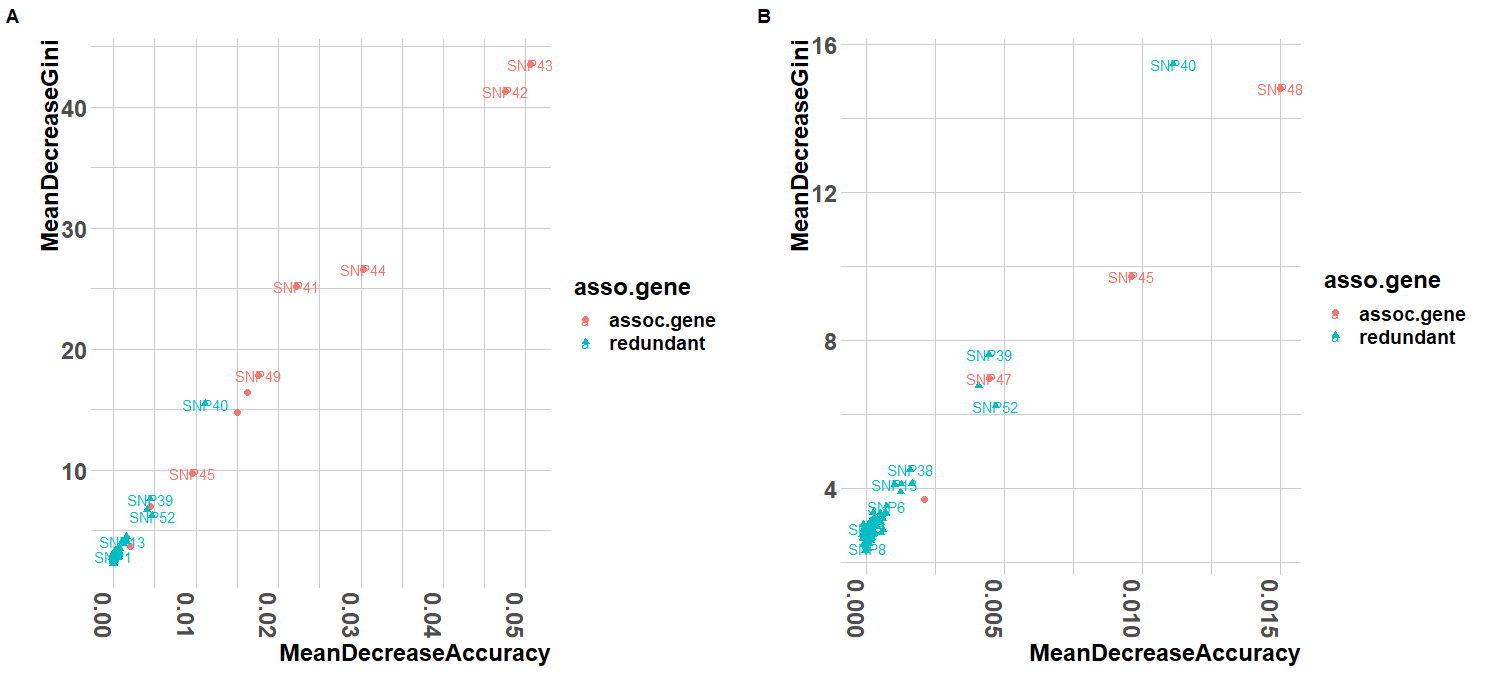
We now turn some observations in according to the missingness mechanism (19), and turn some values to missing as well according to the missingness mechanism
| (22) |
where or 0 depending on whether or not is missing. It is found that the generated data contain 205 missing values. Proportions of missing values in the observations of and are given in Table 6, and their missingness patterns together with that of are summarized in Figure 4. It can be found that the total number of missing values in in Simulation 2 is 1974, and the numbers of individuals having 0, 1, 2, 3, 4, 5, 6, 7 and 8 missing values are 113, 241, 271, 200, 108, 45, 16, 5 and 1, respectively.
| %missing | .236 | .159 | .259 | .141 | .253 | .153 | .245 | .145 | .236 | .147 |
|---|

Next we apply our proposed method to analyze the phenotype-SNP associations using the latest generated and data that contain missing values with non-ignorable missingness mechanism. The procedure and results are described in three parts as following.
Part 1.
We run the Ridge-EM multiple imputations complete data RF variable selection Ridge-EM cycle for times, where the ridge tuning parameter is chosen to minimize the predictive mis-classification error by cross-validation. The cross-validation results are shown in Figure 5, from the top panel of which the best value is found to be in the first run of the cycle; and the best (cf. bottom panel of Figure 5) is found in the tenth run of Ridge-EM when SNPs variable selection is completed. Frequencies of the 100 SNPs being respectively selected by RF for equation (1) out of the 10 cycles are summarized by a circular bar plot displayed in Figure 6. It is shown from Figure 6 that 38 SNPs, including that are used in the data generation and their highly correlated ones (i.e. and ), have their frequencies 10 out of 10. There are 26 SNPs having their frequencies . We include only the former 38 SNPs into the model system (1, 4, 8) for the phenotype-SNP association analysis, which gives the results very similar to those used in Table 5; thus not presented here for brevity of presentation.
We also test the missingness mechanism involved in the above association analysis, with the results provided in Table 7. Note that the term “related SNPs having missing values” in Table 7 refers to those SNPs and phenotype that have missing values and appear in the missingness mechanism model (8). Results in Table 7 show that the missingness mechanisms in SNPs 41 to 45 and are non-ignorable with strong statistical evidences. As an example, Table 7 shows that the missingness of SNP41 is significantly related to SNP45, thus to SNP41 as well because the correlation coefficient between SNP45 and SNP41 is which is a sizeable number. Although the missingness mechanisms for SNPs 1, 2, 3, 4 and 5 are also found to be non-ignorable from Table 7, they are not of our concern because SNPs 1 to 5 are not found to be significantly associated with the phenotype (cf. Figure 6).
Part 2.
We perform two further runs of the Ridge-EM multiple imputations complete data RF variable selection Ridge-EM cycle for and 50 times, respectively. The results on frequencies of each SNP in (1) being selected from the RF in each run are displayed in Figure 7. It can be found from Figure 7 that number of SNPs being selected in each cycle run is 38 when ; 24 when ; and 25 when . This shows that our method has strong capacity to identify all those SNPs that have significant associations with the phenotype, but also has a tendency of over-selection.
| Missingness | Related SNPs having missing values that | Wald test |
| indicators | appear in the missingness mechanism model (8) | -value |
| (SNP1) | 2, 3, 4, 5 | 4.654e-8*** |
| (SNP2) | 3, 4, 44 | 0.00103** |
| (SNP3) | 1, 2, 3, 4, 5 | 8.543e-13*** |
| (SNP4) | 2, 43 | 0.07721 |
| (SNP5) | 3, 4, 5 | 8.142e-11*** |
| (SNP41) | 45 | 0.01916* |
| (SNP42) | 41, 42, 43, 44 | 0.005488*** |
| (SNP43) | 4, 43 | 0.02899 |
| (SNP44) | 41, 42, 43, 44, 45 | 4.209e-5*** |
| (SNP45) | 42, 44 | 0.005264** |
| (phenotype) | 41, 42, | 3.3e-7 |

Part 3.
The same as Part 1 except that EBIC is used to tune the ridge parameter . It is found that the best value is in the first run of the cycle, and is 0.003 in the Ridge-EM after SNP variable selection is completed. The EBIC-based tuning results are shown in Figure 8. Results on the frequencies of each SNP being selected from the RF for (1) in runs of the cycle are summarized by the circular bar plot in Figure 9. From Figure 9 we see 29 SNPs, including SNPs 36 to 55, have full frequency 10; and 35 SNPs have their frequencies . Hence, tuning by EBIC rather than by cross-validation results in less SNPs being selected and more SNPs being removed.
4 Real data application
Now we apply our proposed method to analyze the breast cancer data set introduced at the beginning of Section 2, which comprises 123,372 observations of 207 SNPs on 596 individuals (354 breast cancer patients and 242 matched controls). There are 1,724 missing values in the data, distributions of which over the SNPs and the individuals are summarized in Table 8 and Table 9, respectively. The pairwise LD structure of the 207 SNPs is displayed in Figure 10 where single imputation for missing values is used in the left plot and multiple imputations are used in the right one. Figure 10 shows that, as the distance between any two SNPs increases, the dependence between them would decrease. On the other hand, there exists strong dependence between adjacent SNPs.
| Range of numbers | 0 | 1-9 | 10-19 | 20-29 | 30-32 |
|---|---|---|---|---|---|
| of missing values | |||||
| Number of SNPs | 50 | 81 | 44 | 30 | 2 |
| Range of numbers | 0 | 1 | 2 | 3 | 4 | 5 | 6 | 7 | 8 | 9 |
| of missing values | ||||||||||
| Number of individuals | 83 | 107 | 132 | 79 | 59 | 44 | 31 | 30 | 15 | 16 |
The Ridge-EM multiple imputations complete data RF variable selection Ridge-EM cycle is run times, resulting in 16 SNPs being selected in each run, which can be determined from the circular frequency map in Figure 11 and also are listed in Table 10. It is found that 11 of the 16 selected SNPs, which are displayed in parentheses in Tabele 10, contain missing values. In this analysis, each SNP variable is coded with two dummy variables as in Simulation 1. Since many of the SNPs having missing values have just a few missing values (cf. Table 8), we used the bias-reduction estimation method of Firth (1993) and the corresponding R package brglm Kosmidis & Kosmidis (2020) in each fitting of (1,4,8). Also there is no need to use ridge regression for this particular data set. In other words, using is sufficient for having convergent parameter estimates.
We now use the breast cancer data, together with the multiple imputations of the missing values, to fit the logistic model (1) where only the 16 selected SNPs are included as covariates. Results on the parameter estimation in model (1) are summarized in the left panel of Table 10. For comparison, we fit the same logistic model to the same breast cancer data but the involved missing values are excluded from fitting. The results are shown in the right panel in Table 10. Comparing the left panel with the right one in Table 10 we see rs2547231C is significantly associated with the breast cancer risk in both panels; rs1004984A is more significant in the left panel than in the right panel; rs1845557C is significant at level 0.1 in the left panel but not significant in the right panel; and rs6902771T is significant in the left panel but not in the right one. The other SNPs do not seem to be significant in either the panel. Therefore, by using multiple imputations to account for the effect of missing values we are able to find some significant SNPs that can not be found by using only the observed data to fit the model. There should be more analysis on whether any redundant SNPs can be further removed from the model (1) for the breast cancer data. But it would be beyond the scope of this research.
To see whether the missingness mechanism can be ignored for each of the 11 SNPs listed in Table 10 and having missing values, we fit model (8) for these 11 SNPs as part of the whole process. The results are summarized in Table 11, from which we see all the 11 SNPs, except rs1131878C and rs2547231C, have non-ignorable missingness mechanism. Here we say a SNP rsxxx has non-ignorable missingness mechanism if the missingness indicator (rsxxx) is significantly associated with any SNPs having missing values or with missingness indicators of any other SNPs.
| MI-RF based | Observed data based | |||||
| Coefficients | Estimate | Std.Err | Pr() | Estimate | Std.Err | Pr() |
| Intercept | -0.165 | 0.515 | 0.748 | 0.143 | 0.539 | 0.791 |
| 0.393 | 0.196 | 0.045 | 0.365 | 0.206 | 0.077 | |
| 0.200 | 0.279 | 0.473 | 0.252 | 0.292 | 0.387 | |
| 0.275 | 0.192 | 0.152 | 0.287 | 0.201 | 0.154 | |
| -0.034 | 0.326 | 0.916 | 0.052 | 0.345 | 0.881 | |
| -0.242 | 0.197 | 0.219 | -0.200 | 0.208 | 0.335 | |
| -0.305 | 0.270 | 0.259 | -0.271 | 0.282 | 0.337 | |
| 0.050 | 0.191 | 0.792 | 0.036 | 0.202 | 0.857 | |
| -0.516 | 0.304 | 0.09 | -0.503 | 0.318 | 0.113 | |
| 0.268 | 0.217 | 0.216 | 0.177 | 0.226 | 0.433 | |
| 0.072 | 0.312 | 0.817 | -0.033 | 0.325 | 0.919 | |
| -0.049 | 0.209 | 0.816 | 0.013 | 0.217 | 0.951 | |
| -0.324 | 0.260 | 0.213 | -0.226 | 0.275 | 0.412 | |
| ) | 0.130 | 0.287 | 0.651 | 0.112 | 0.302 | 0.711 |
| 0.502 | 0.376 | 0.182 | 0.357 | 0.399 | 0.371 | |
| -0.726 | 0.196 | 0.0002 | -0.683 | 0.204 | 0.0008 | |
| 0.418 | 0.724 | 0.564 | 0.041 | 0.751 | 0.956 | |
| -0.345 | 0.219 | 0.115 | -0.341 | 0.232 | 0.143 | |
| -0.381 | 0.250 | 0.128 | -0.430 | 0.263 | 0.102 | |
| 0.075 | 0.213 | 0.723 | -0.045 | 0.225 | 0.843 | |
| 0.300 | 0.252 | 0.234 | 0.115 | 0.263 | 0.662 | |
| 0.285 | 0.211 | 0.177 | 0.328 | 0.220 | 0.135 | |
| 0.257 | 0.251 | 0.305 | 0.146 | 0.261 | 0.577 | |
| 0.491 | 0.774 | 0.526 | -0.220 | 0.898 | 0.806 | |
| 0.060 | 1.032 | 0.954 | -0.741 | 1.196 | 0.536 | |
| 0.175 | 0.217 | 0.421 | 0.156 | 0.226 | 0.491 | |
| 0.288 | 0.310 | 0.354 | 0.233 | 0.324 | 0.473 | |
| -0.131 | 0.194 | 0.500 | -0.067 | 0.205 | 0.745 | |
| -0.359 | 0.268 | 0.181 | -0.365 | 0.277 | 0.188 | |
| 0.434 | 0.207 | 0.036 | 0.307 | 0.218 | 0.158 | |
| 0.031 | 0.253 | 0.902 | -0.028 | 0.264 | 0.916 | |
| -0.498 | 0.753 | 0.509 | 0.097 | 0.873 | 0.912 | |
| 0.846 | 1.026 | 0.409 | 1.442 | 1.185 | 0.224 | |
| AIC: 654.74 | AIC: 737.13 | |||||
| Coefficient | Estimate | Std.Error | Z value | Pr() |
|---|---|---|---|---|
| Testing the missingness mechanism of | ||||
| Intercept | -6.659 | 1.472 | -4.525 | 6.05e-6 |
| -0.466 | 1.716 | -2.272 | 0.786 | |
| 1.724 | 1.473 | 1.170 | 0.242 | |
| 1.157 | 1.615 | 0.716 | 0.474 | |
| 4.236 | 1.463 | 2.895 | 0.004 | |
| Testing the missingness mechanism of | ||||
| Intercept | -5.900 | 1.420 | -4.155 | 3.26e-5 |
| -0.472 | 2.007 | -0.235 | 0.814 | |
| 1.505 | 1.642 | 0.917 | 0.359 | |
| Testing the missingness mechanism of | ||||
| Intercept | -5.822 | 1.149 | -5.068 | 4.02e-7 |
| 1.268 | 1.366 | 0.928 | 0.353 | |
| 0.261 | 0.857 | 0.305 | 0.760 | |
| 1.236 | 1.022 | 1.210 | 0.226 | |
| -3.355 | 0.905 | -0.392 | 0.695 | |
| 0.521 | 1.029 | 0.507 | 0.613 | |
| 0.417 | 0.832 | 0.501 | 0.616 | |
| 1.338 | 1.491 | 0.897 | 0.370 | |
| 0.259 | 0.902 | 0.287 | 0.774 | |
| 1.544 | 1.248 | 1.237 | 0.216 | |
| 0.242 | 0.861 | 0.281 | 0.779 | |
| 0.828 | 1.051 | 0.788 | 0.431 | |
| 0.321 | 0.887 | 0.362 | 0.717 | |
| 1.808 | 1.213 | 1.491 | 0.136 | |
| 1.932 | 1.494 | 1.293 | 0.196 | |
| -1.119 | 2.143 | -0.522 | 0.602 | |
| 0.661 | 0.895 | 0.739 | 0.460 | |
| 2.563 | 1.813 | 1.414 | 0.157 | |
| 3.303 | 2.087 | 1.583 | 0.113 | |
| 4.395 | 1.598 | 2.751 | 0.00594 | |
| Table 11 continued | ||||
|---|---|---|---|---|
| Coefficient | Estimate | Std.Error | Z value | Pr() |
| Testing the missingness mechanism of | ||||
| Intercept | -5.098 | 1.320 | -3.861 | 0.0001 |
| -3.974 | 2.167 | -1.834 | 0.067 | |
| -2.897 | 2.913 | -0.994 | 0.320 | |
| 0.025 | 1.365 | 0.018 | 0.986 | |
| 0.453 | 1.599 | 0.283 | 0.777 | |
| 3.628 | 1.228 | 2.955 | 0.003 | |
| 1.718 | 2.107 | 0.815 | 0.415 | |
| 0.931 | 0.706 | 1.319 | 0.187 | |
| -0.680 | 1.390 | -0.489 | 0.625 | |
| 0.970 | 1.007 | 0.964 | 0.335 | |
| 1.310 | 1.509 | 0.868 | 0.385 | |
| -0.713 | 1.312 | -0.544 | 0.587 | |
| 0.568 | 2.001 | 0.284 | 0.776 | |
| 2.941 | 1.505 | 1.953 | 0.051 | |
| 3.520 | 1.160 | 3.034 | 0.002 | |
| -0.512 | 4.122 | 0.124 | 0.901 | |
| -3.484 | 3.305 | -1.054 | 0.292 | |
| 0.110 | 0.938 | 0.117 | 0.907 | |
| 3.005 | 1.228 | 2.448 | 0.014 | |
| 0.811 | 2.033 | 0.399 | 0.690 | |
| 3.814 | 3.071 | 1.242 | 0.214 | |
| -4.920 | 1.362 | -3.611 | 0.0003 | |
| -2.229 | 1.891 | -1.179 | 0.239 | |
| -0.413 | 2.014 | -0.205 | 0.837 | |
| 1.400 | 3.267 | 0.428 | 0.668 | |
| 2.104 | 0.843 | 2.497 | 0.012 | |
| 4.182 | 2.019 | 2.071 | 0.038 | |
| 3.393 | 2.157 | 1.573 | 0.116 | |
| 2.756 | 3.037 | 0.907 | 0.364 | |
| -0.478 | 0.784 | -0.609 | 0.542 | |
| 2.521 | 1.245 | 2.025 | 0.043 | |
| -1.626 | 4.039 | -0.397 | 0.691 | |
| 3.261 | 3.198 | 1.020 | 0.308 | |
| 1.500 | 1.007 | 1.489 | 0.137 | |
| -2.193 | 2.828 | -0.775 | 0.438 | |
| Table 11 continued | ||||
|---|---|---|---|---|
| Coefficient | Estimate | Std.Error | Z value | Pr() |
| Testing the missingness mechanism of | ||||
| Intercept | -6.543 | 1.140 | -5.740 | 9.45e-9 |
| 4.328 | 1.598 | 2.708 | 0.007 | |
| 1.422 | 1.603 | 0.887 | 0.375 | |
| 0.902 | 0.713 | 1.266 | 0.205 | |
| 2.483 | 1.121 | 2.214 | 0.027 | |
| -0.654 | 0.786 | -0.833 | 0.405 | |
| 2.222 | 0.987 | 2.252 | 0.024 | |
| -3.176 | 1.871 | -1.698 | 0.090 | |
| -4.161 | 2.533 | -1.643 | 0.100 | |
| 2.392 | 1.997 | 1.198 | 0.231 | |
| 6.160 | 2.995 | 2.056 | 0.040 | |
| 2.052 | 0.738 | 2.779 | 0.005 | |
| 3.824 | 1.878 | 2.036 | 0.042 | |
| 2.185 | 1.428 | 1.529 | 0.126 | |
| 9.910 | 2.396 | 2.468 | 0.014 | |
| Testing the missingness mechanism of | ||||
| Intercept | -5.952 | 1.205 | -4.937 | 7.92e-7 |
| 5.958 | 2.125 | 2.803 | 0.005 | |
| 3.026 | 1.593 | 1.900 | 0.057 | |
| 5.984 | 1.531 | 3.908 | 9.31e-5 | |
| -1.104 | 2.667 | -0.414 | 0.679 | |
| -0.631 | 1.503 | -0.433 | 0.665 | |
| 0.913 | 1.379 | 0.662 | 0.508 | |
| -1.897 | 1.433 | -1.324 | 0.185 | |
| 3.135 | 1.296 | 2.419 | 0.016 | |
| Testing the missingness mechanism of | ||||
| Intercept | -7.061 | 1.640 | -4.307 | 1.65e-5 |
| -0.509 | 1.072 | -0.475 | 0.635 | |
| 0.442 | 1.173 | 0.377 | 0.706 | |
| 3.197 | 1.645 | 1.944 | 0.052 | |
| 5.401 | 2.613 | 2.067 | 0.039 | |
| -1.492 | 1.550 | -0.963 | 0.336 | |
| -1.251 | 2.454 | -0.510 | 0.610 | |
| -0.344 | 1.177 | -0.293 | 0.770 | |
| 1.956 | 1.030 | 1.899 | 0.058 | |
| 1.342 | 1.324 | 1.013 | 0.311 | |
| 4.014 | 1.594 | 2.518 | 0.012 | |
| Table 11 continued | ||||
|---|---|---|---|---|
| Coefficient | Estimate | Std.Error | Z value | Pr() |
| Testing the missingness mechanism of | ||||
| Intercept | -2.388 | 1.498 | -4.931 | 8.2e-7 |
| 5.033 | 1.548 | 3.252 | 0.001 | |
| 4.455 | 1.983 | 2.246 | 0.025 | |
| 4.160 | 1.809 | 2.300 | 0.021 | |
| 0.016 | 1.466 | 0.011 | 0.001 | |
| 3.484 | 1.797 | 1.939 | 0.053 | |
| Testing the missingness mechanism of | ||||
| Intercept | -2.694 | 0.479 | -5.621 | 1.9e-8 |
| -0.315 | 0.479 | -0.658 | 0.511 | |
| 1.849 | 0.826 | 2.239 | 0.025 | |
| 1.001 | 0.479 | 2.091 | 0.037 | |
| 2.370 | 1.248 | 1.898 | 0.058 | |
| -0.902 | 0.443 | -2.037 | 0.042 | |
| -1.092 | 0.540 | -2.023 | 0.043 | |
| -0.733 | 0.528 | -1.388 | 0.165 | |
| 1.465 | 0.755 | 1.942 | 0.052 | |
| -0.913 | 0.447 | -2.044 | 0.041 | |
| -0.221 | 0.666 | -0.331 | 0.740 | |
| 1.441 | 0.439 | 3.283 | 0.001 | |
| -0.158 | 1.482 | -0.107 | 0.915 | |
| Testing the missingness mechanism of | ||||
| Intercept | -6.864 | 1.203 | -5.704 | 1.17e-8 |
| 2.592 | 1.857 | 1.395 | 0.163 | |
| 2.291 | 2.434 | 0.941 | 0.347 | |
| 6.6614 | 2.060 | 3.234 | 0.001 | |
| 1.4586 | 2.091 | 0.698 | 0.485 | |
| 0.404 | 1.754 | 0.230 | 0.818 | |
| Testing the missingness mechanism of | ||||
| Intercept | -9.833 | 2.377 | -4.137 | 3.52e-5 |
| 5.240 | 1.802 | 2.908 | 0.004 | |
| 2.643 | 1.146 | 2.306 | 0.021 | |
| 3.317 | 1.245 | 2.664 | 0.008 | |
| 2.276 | 1.954 | 1.165 | 0.244 | |
| 2.817 | 1.047 | 1.376 | 0.169 | |
| 1.203 | 1.434 | 0.839 | 0.402 | |
| 3.351 | 1.602 | 2.092 | 0.036 | |
| -0.161 | 1.419 | -0.113 | 0.910 | |
| 1.785 | 1.341 | 1.330 | 0.183 | |
5 Discussion
High dimensionality, high correlations, and widespread missing values with non-ignorable missingness mechanisms are the three challenges present in GWAS. The main contribution of this paper is the development of a coherent statistical procedure of categorical phenotype-genotype association analysis, integrating the state-of-the-art methods of random forest for variable selection, weighted ridge regression with EM algorithm for missing data imputation, and linear statistical hypothesis testing for determining the missingness mechanism. Two simulated GWASs have been carried out to assess the performance of the proposed procedure, followed by a real data analysis on breast cancer GWAS for illustration.
The statistical methods used to develop our Ridge-EM multiple imputations complete data RF variable selection Ridge-EM procedure are well established and implemented into several statistical computing environments. But integrating them to tackle GWAS data analysis involving missing values with non-ignorable missingness mechanism is not trivial but requires dedicated efforts. For example, the GeneSrF method by Díaz-Uriarte & De Andres (2006) is not able to handle non-uniform high-dimensional imputation weights that are commonly present in missing data analysis. We have overcome this difficulty by applying the fast algorithm of Wright & Ziegler (2015) to implement GeneSrF, and have obtained satisfactory outcomes. As another example, multiple imputation techniques have been used in GWAS to replace the missing values by surrogates; but the existing practice stops going further to investigate whether the missingness mechanism is ignorable or not. We are able to test whether or not the missingness mechanism is ignorable by applying a standard statistical linear hypothesis testing procedure. This is only possible after we establish the model system (1, 4, 8) for GWAS.
It has been observed that our developed method would become computationally very intensive if the proportions of missing values in relevant SNPs are very high and number of such SNPs is also high, because of the combinatorial explosion involved in multiple imputation and variable selection. A promising solution to this difficulty is to incorporate Markov chain Monte Carlo into the EM algorithm, and to perform variable selection by stochastic search. We are currently working on this solution, and will report the results somewhere else once available.
References
- Baker & Laird ((1988)) Baker, S.G. & Laird, N.M. (1988). Regression analysis for categorical variables with outcome subject to nonignorable nonresponse. Journal of the American Statistical association 83 401 62–69.
- Breiman ((2001)) Breiman, L. (2001). Random forests. Machine learning 45 1 5–32.
- Calle et al. ((2011)) Calle, M.L., Urrea, V., Boulesteix, A-L. & Malats, N. (2011). Auc-rf: a new strategy for genomic profiling with random forest. Human heredity 72 2 121–132.
- Chen & Ishwaran ((2012)) Chen, X. & Ishwaran, H. (2012). Random forests for genomic data analysis. Genomics 99 6 323–329.
- Craven & Wahba ((1978)) Craven, P. & Wahba, G. (1978). Smoothing noisy data with spline functions: Estimating the correct degree of smoothing by the method of generalized crossvalidation. Numerische Mathematik 31 4 377–403.
- Dempster et al. ((1977)) Dempster, A.P., Laird, N.M. & Rubin, D.B. (1977). Maximum likelihood from incomplete data via the em algorithm. Journal of the Royal Statistical Society: Series B (Statistical Methodology) 39 1 1–38.
- Díaz-Uriarte & De Andres ((2006)) Díaz-Uriarte, R. & De Andres, S.A. (2006). Gene selection and classification of microarray data using random forest. BMC bioinformatics 7 1 3.
- Dite et al. ((2003)) Dite, G.S., Jenkins, M.A., Southey, M.C., Hocking, J.S., Giles, G.G., McCredie, M.R.Hopper, J.L. (2003). Familial risks, early-onset breast cancer, and brca1 and brca2 germline mutations. Journal of the National Cancer Institute 95 6 448–457.
- Firth ((1993)) Firth, D. (1993). Bias reduction of maximum likelihood estimates. Biometrika 80 1 27–38.
- Foulkes ((2009)) Foulkes, A.S. (2009). Applied statistical genetics with r. : Springer.
- Gauderman et al. ((2007)) Gauderman, W.J., Murcray, C., Gilliland, F. & Conti, D.V. (2007). Testing association between disease and multiple snps in a candidate gene. Genetic Epidemiology: The Official Publication of the International Genetic Epidemiology Society 31 5 383–395.
- Grund et al. ((2016)) Grund, S., Lüdtke, O. & Robitzsch, A. (2016). Multiple imputation of multilevel missing data: An introduction to the r package pan. Sage Open 6 4 2158244016668220.
- Hoerl & Kennard ((1981)) Hoerl, A.E. & Kennard, R.W. (1981). Ridge regression—1980: Advances, algorithms, and applications. American Journal of Mathematical and Management Sciences 1 1 5–83.
- Ibrahim et al. ((1999)) Ibrahim, J.G., Lipsitz, S.R. & Chen, M-H. (1999). Missing covariates in generalized linear models when the missing data mechanism is non-ignorable. Journal of the Royal Statistical Society: Series B (Statistical Methodology) 61 1 173–190.
- Jiang et al. ((2004)) Jiang, H., Deng, Y., Chen, H-S., Tao, L., Sha, Q., Chen, J.Zhang, S. (2004). Joint analysis of two microarray gene-expression data sets to select lung adenocarcinoma marker genes. BMC bioinformatics 5 1 81.
- Kosmidis & Kosmidis ((2020)) Kosmidis, I. & Kosmidis, M.I. (2020). Package ‘brglm’. URL: https://cran. r-project. org/web/packages/brglm2/brglm2. pdf (last accessed 22 Sep. 2020) .
- Lipsitz & Ibrahim ((1996)) Lipsitz, S.R. & Ibrahim, J.G. (1996). A conditional model for incomplete covariates in parametric regression models. Biometrika 83 4 916–922.
- Louis ((1982)) Louis, T.A. (1982). Finding the observed information matrix when using the em algorithm. Journal of the Royal Statistical Society: Series B (Statistical Methodology) 44 2 226–233.
- Marchini et al. ((2007)) Marchini, J., Howie, B., Myers, S., McVean, G. & Donnelly, P. (2007). A new multipoint method for genome-wide association studies by imputation of genotypes. Nature genetics 39 7 906–913.
- Odefrey et al. ((2010)) Odefrey, F., Stone, J., Gurrin, L.C., Byrnes, G.B., Apicella, C., Dite, G.S.Study, S.M.D. (2010). Common genetic variants associated with breast cancer and mammographic density measures that predict disease. Cancer Research 70 4 1449–1458.
- Olkin & Tate ((1961)) Olkin, I. & Tate, R.F. (1961). Multivariate correlation models with mixed discrete and continuous variables. The Annals of Mathematical Statistics 32 2 448–465.
- Qian et al. ((2019)) Qian, G., Wu, Y. & Xu, M. (2019). Multiple change-points detection by empirical bayesian information criteria and gibbs sampling induced stochastic search. Applied Mathematical Modelling 72 8 202–216.
- Sabbe et al. ((2013)) Sabbe, N., Thas, O. & Ottoy, J-P. (2013). Emlasso: logistic lasso with missing data. Statistics in medicine 32 18 3143–3157.
- Scheet & Stephens ((2006)) Scheet, P. & Stephens, M. (2006). A fast and flexible statistical model for large-scale population genotype data: applications to inferring missing genotypes and haplotypic phase. The American Journal of Human Genetics 78 4 629–644.
- Schwarz ((1978)) Schwarz, G.E. (1978). Estimating the dimension of a model. The Annals of Statistics 6 2 461–464.
- Stubbendick & Ibrahim ((2003)) Stubbendick, A.L. & Ibrahim, J.G. (2003). Maximum likelihood methods for nonignorable missing responses and covariates in random effects models. Biometrics 59 4 1140–1150.
- Tibshirani ((1996)) Tibshirani, R. (1996). Regression shrinkage and selection via the lasso. Journal of the Royal Statistical Society: Series B (Methodological) 58 1 267–288.
- Wright & Ziegler ((2015)) Wright, M.N. & Ziegler, A. (2015). ranger: A fast implementation of random forests for high dimensional data in c++ and r. arXiv preprint arXiv:1508.04409 .
- Zou & Hastie ((2005)) Zou, H. & Hastie, T. (2005). Regularization and variable selection via the elastic net. Journal of the royal statistical society: series B (statistical methodology) 67 2 301–320.