How perturbative QCD constrains the Equation of State at Neutron-Star densities
Abstract
We demonstrate in a general and analytic way how high-density information about the equation of state (EoS) of strongly interacting matter obtained using perturbative Quantum Chromodynamics (pQCD) constrains the same EoS at densities reachable in physical neutron stars. Our approach is based on utilizing the full information of the thermodynamic potentials at the high-density limit together with thermodynamic stability and causality. This requires considering the pressure as a function of chemical potential instead of the commonly used pressure as a function of energy density . The results can be used to propagate the pQCD calculations reliable around 40 to lower densities in the most conservative way possible. We constrain the EoS starting from only few times the nuclear saturation density and at we exclude at least 65% of otherwise allowed area in the -plane. This provides information complementary to astrophysical observations that should be taken into account in any complete statistical inference study of the EoS. These purely theoretical results are independent of astrophysical neutron-star input, and hence, they can also be used to test theories of modified gravity and BSM physics in neutron stars.
I Introduction
The rapid evolution of neutron-star (NS) astronomy — in particular, the recent NS radius measurements Miller et al. 2021; Riley et al. 2021, the discovery of massive NSs Demorest et al. 2010; Antoniadis et al. 2013; Fonseca et al. 2021, and the advent of gravitational-wave and multi-messenger astronomy Abbott et al. 2017a; Abbott et al. 2017b — is for the first time giving us empirical access to the physics of the cores of NSs. Within the Standard Model and assuming general relativity, the internal structure of NSs is determined by the equation of state (EoS) of strongly interacting matter Tolman 1939; Oppenheimer and Volkoff 1939. With these assumptions, NS observations can be used to empirically determine the EoS Annala et al. 2018; Margalit and Metzger 2017; Rezzolla et al. 2018; Ruiz et al. 2018; Bauswein et al. 2017; Radice et al. 2018; Most et al. 2018; Dietrich et al. 2020; Capano et al. 2020; Landry and Essick 2019; Raithel et al. 2018; Raithel and Özel 2019; Raaijmakers et al. 2020; Essick et al. 2020; Al-Mamun et al. 2021; Essick et al. 2021; Paschalidis et al. 2018; Annala et al. 2020; Ferreira et al. 2020; Minamikawa et al. 2021; Blacker et al. 2020 (for reviews, see Baym et al. 2018; Gandolfi et al. 2019; Raithel 2019; Horowitz 2019; Baiotti 2019; Chatziioannou 2020; Radice et al. 2020). And if the EoS can be determined theoretically to a sufficient accuracy, comparison with NS observations allows to use these extreme objects as laboratory for physics beyond the standard model (e.g., Goldman and Nussinov 1989; Giudice et al. 2016; Ciarcelluti and Sandin 2011; Li et al. 2012; Xiang et al. 2014; Tolos and Schaffner-Bielich 2015; Ellis et al. 2018; Del Popolo et al. 2020; Jiménez and Fraga 2021) and/or general relativity (e.g., Damour and Esposito-Farese 1993; He et al. 2015; Aparicio Resco et al. 2016; Doneva et al. 2018; Lope Oter et al. 2019).
For both of these goals, it is crucial to make use of all possible controlled theory calculations that inform us about the EoS at densities reached in NSs. While in principle the EoS is determined by the underlying theory of strong interactions, Quantum Chromodynamics (QCD), in practice we have access to the EoS only in limiting cases. In the context of low temperatures relevant for neutron stars, the EoS of QCD can be systematically approximated at low- and at high-density limits. At low densities, the current state-of-the-art low-energy effective theory calculations allow to describe matter to densities around and slightly above nuclear saturation density Tews et al. 2013; Drischler et al. 2019, but become unreliable at higher densities reached in the cores of massive neutron stars. A complementary description of NS matter comes from perturbative QCD (pQCD) calculations which become reliable at sufficiently high densities , far exceeding those realised in NSs Gorda et al. 2018; Gorda et al. 2021.
Several works have used large ensembles of parameterized EoSs to study the possible behavior of the EoS in intermediate densities between the theoretically known limits. Many of these works have anchored their EoS to the low-density limit only, while others have interpolated between the two orders of magnitude in density separating the low- and high-density limits Kurkela et al. 2014; Annala et al. 2018; Most et al. 2018; Annala et al. 2020; Annala et al. 2021. While the input from pQCD clearly constrains the EoS at very high densities, how this information affects the EoS around neutron-star densities has so far been convoluted by the specific choices of interpolation functions.
The aim of the present work is to make the influence of the high-density calculations to the EoS at intermediate densities explicit, and in particular, to derive constraints to the EoS that are completely independent of any specific interpolation function. By using the full information available in the thermodynamic grand canonical potential as a function of baryon chemical potential, , we find stricter bounds than works using only the reduced form of the EoS, i.e., the pressure as a function of the energy density appearing in the hydrodynamic description of neutron-star matter Rhoades and Ruffini 1974; Koranda et al. 1997; Lope Oter et al. 2019; Tews et al. 2019; Lope-Oter and Llanes-Estrada 2021. The effect is demonstrated in fig. 1, which shows the region in -plane that can be reached with a causal and thermodynamically stable EoS with information of the high-density limit, and in particular compares the allowed values at different fixed densities with and without the pQCD input.
II setup
In the following we consider all possible interpolations of the full thermodynamic potential at zero temperature and in -equilibrium, , between the low-density limit and the high-density limit . We assume that at both of these limits the pressure and its first derivative, baryon number density are now
| (1) | ||||
| (2) |
This information is readily available from the microscopic calculations which are assumed to be reliable at these limits; representative values from state-of-the-art chiral effective theory (CET) Hebeler et al. 2013 and pQCD calculations Gorda et al. 2021 from the literature are reproduced in table 1 11 1 In addition to the perturbative contribution, the pressure at high densities may also receive a non-pertrubative, density independent contribution often referred as the bag constant. We have checked that inclusion of a bag constant of MeV/fm3 leads to an effect that is qualitatively similar but negligible in size compared to scale variation error..
Thermodynamic consistency requires that pressure is a continuous function of . Similarly, thermodynamic stability requires concavity of thermodynamic potentials so that is a monotonically increasing function . Density does not need to be continuous and it can have discontinuities (increasing the density at fixed ) in the case of first-order phase transitions; we place no additional assumptions on the number or strength of possible transitions. Causality requires that the speed of sound is less than the speed of light, , and it imposes a condition on the first derivative of .
| (3) |
| CET | pQCD | ||||
|---|---|---|---|---|---|
| soft | stiff | ||||
| [GeV] | 0.966 | 0.978 | 2.6 | ||
| [1/fm3] | 0.176 | 6.14 | 6.47 | 6.87 | |
| [MeV/fm3] | 2.163 | 3.542 | 2334. | 3823. | 4284. |
We construct the allowed EoSs by considering all possible functions allowed by the above assumptions connecting the low- and high-density limits. Causality imposes a minimal slope, , that any causal EoS passing though a given point in the plane can have. This is visualized as a vector field, where the arrows at each point correspond to tangent lines with constant . This requirement imposes two fundamental constraints. Starting from the point we can follow the arrows until by solving eq. 3 with , leading to . This produces a maximally stiff causal EoS and the area under this line cannot be reached from the low-density limit with a causal EoS. Correspondingly, the upper limit for the can be obtained starting from and following the arrows backward to ; the high-density limit cannot be reached from any point above this line by a causal EoS. These previously known bounds (e.g. Rhoades and Ruffini 1974; Lope Oter et al. 2019) are represented as orange lines in fig. 2.
The simultaneous requirement of reaching both and imposes further constraints and fixes the area under the curve
| (4) |
In the example shown in fig. 2, this requirement imposes that the area under any allowed EoS is approximately one third the area of the figure.
At each point, we can evaluate the absolute minimum and maximum area under any EoS () that can be reached at if the EoS goes through that particular point. If () is bigger (smaller) than , then such a point would be ruled out.
To obtain the minimum area at for any EoS going through a specific point consider the following construction shown in fig. 2 as a dashed blue line:
For , the smallest possible area is determined by the maximally stiff causal line (i.e. ) starting from which we follow up to . At , we have a phase transition where the density jumps to . After that, the EoS follows the maximally stiff causal line starting at until , where the EoS has another phase transition to reach . The solution to the equation is shown in fig. 2 as the top red line denoted integral constraints; any EoS crossing this line is inconsistent with simultaneous constraint on and . This yields a maximum density for given ,
where is given by the intercept of the causal line and the integral constraint, i.e., the two cases in section II,
| (9) |
Similarly, the procedure to maximize area under any EoS going through the point is shown as a dashed green line in fig. 2,
Correspondingly, solving for gives a constraint to the minimal that can be obtained for a given , depicted as the bottom red line in fig. 2. Then, for a given chemical potential the minimal allowed density is
Note that the point of interception is the same for the upper and lower limits. This happens because the EoS following up to obtains the correct area only if the EoS jumps at from to . This is also the EoS exhibiting a phase transition with the largest possible latent heat
| (14) |
Further, we denote the special EoS with throughout the whole region as
| (15) |
Any point along this line maximises the area to the left of the point () and minimizes to the right of the point (), so that this line corresponds to the maximal pressure at fixed .
III Mapping to the plane
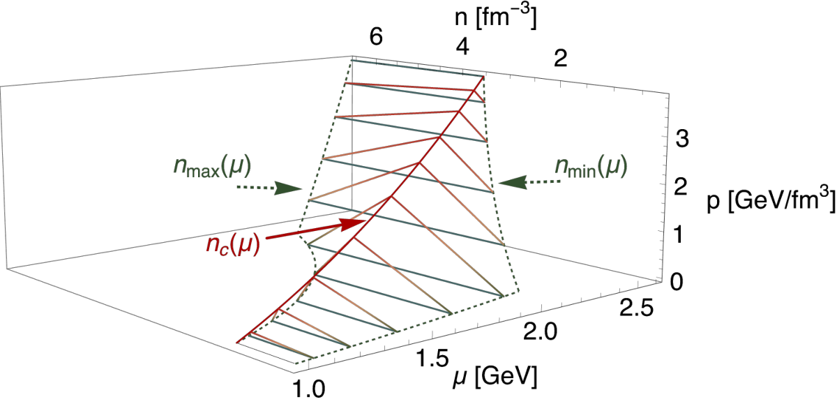
For every allowed point on the -plane, we can find minimal and maximal pressures, , that can be obtained at that point . Note that this is different from the minimal and maximal pressures () obtainable at by an EoS passing though , as discussed in the previous section.
The minimal pressure is given by the EoS that follows the maximally stiff causal line terminating at the point , i.e., , and has a phase transition from to at . This construction leads to a lower bound of the pressure as function of and
| (16) |
In order to find the maximal pressure for a given point, the plane needs to be divided in two different regions. For (see eq. 15), the maximal pressure is obtained by following the maximally stiff causal line terminating at the point itself
| (17) |
For , the above construction would lead to a phase transition at CET point that is inconsistent with the upper integral constraints. Instead, a bound can be obtained by noting that the EoS that maximizes the pressure at is an EoS that minimizes the pressure difference between and . Thus the maximum pressure at that point is given by the difference between and the pressure for the maximally stiff EoS following the causal line starting at
| (18) |
The simultaneous bounds for , and are visualized in fig. 3. These constraints can be easily translated into bounds on the -plane using the Euler equation for a fixed density . An analytic solution for the envelope of the allowed values of irrespective of (green lines in fig. 1 and fig. 4) is given in supplemental material.
Figure 1 shows the allowed range of and values with and without imposing the high-density constraint for fixed densities of and using the standard central renormalization scale commonly used in the literature Schneider 2003; Ipp and Rebhan 2003; Fraga and Romatschke 2005, , for pQCD and the ”stiff” values for CET. At the density of , the high-density input does not offer additional constraint. However, strikingly, already at the largest pressures are cut off by the integral constraint and only 68 of the values remain (given by the ratio of the blue and combined blue and red areas in fig. 1 when plotted in linear scale). At only of the allowed region remains whereas at , the allowed range of values is significantly reduced, now also featuring a cut of the lowest pressures leaving around 6.5 of the total area.
We have checked the stability of these results against the variation of different pQCD and CET limits in table 1. While varying the CET parameters has a very small effect on the excluded areas (of the order of line width in fig. 1), varying the pQCD renormalization parameter increases the area in -plane. The effect of varying is shown in fig. A1 of the Supplemental Material. The union of allowed areas in range excludes of the otherwise allowed area (without pQCD) for . The lowest density at which and are limited by the high-density input from above is and from below is for .
IV Speed-of-sound constraints
The EoSs that render the boundaries of the allowed regions in fig. 1 and fig. 2 are composed of the most extreme ones. They contain maximal allowed phase transitions and extended density ranges where . While it is clear that these most extreme EoSs are unlikely to be the physical one, they cannot be excluded with the same level of robustness as those which break the above criteria.
A possible way to quantify how extreme the EoSs are is by imposing a maximal speed of sound that is reached at any density within the interpolation region Annala et al. 2020. In supplemental material we give the generalizations for , , and for arbitrary limiting .
As the maximum speed of sound is reduced, the allowed range of possible diminishes rapidly leading to tighter bounds on the EoS. This is demonstrated in fig. 4 showing the range of allowed values of at different values of . Interestingly, while the so-called conformal bound — that is, — is consistent with the high-density constraint, imposing this condition gives an extremely strong constraint and forces the EoS to have a specific shape at all densities.
Decreasing even further, we eventually close the gap between the lower and upper bounds completely, shown in fig. 4 as a red line. At this specific value of the allowed region degenerates into a single line. This is the minimum limiting value for sound speed for which the low- and high- density limits can be connected in a consistent way. Thus has to be reached by any EoS at some density. For , we get , just below the asymptotic conformal value of pQCD.
V Discussions
Our results demonstrate the nontrivial and robust constraints on the EoS at NS densities arising from pQCD calculations. These constraints are obtained only when interpolating the full EoS instead of its reduced form .
In order to demonstrate the practical utility of the results we have checked the consistency of the large number of publicly available EoSs Typel et al. 2015; Oertel et al. 2017 against new constraints; see fig. A2 in the Supplemental Material.
The results highlight the complementarity of the high- and low-density calculations. This is further demonstrated in fig. 5 depicting the expected effect of future calculations on the allowed region of -values at and . We anticipate future results by extrapolating either CET (”stiff”) up to using values tabulated in Hebeler et al. 2013 and/or extrapolating the pQCD results () of Gorda et al. 2021 down to (corresponding to GeV). Improvements of this magnitude have been suggested, e.g., in Fujimoto and Fukushima 2020; Fernandez and Kneur 2021. We see that both the low- and the high-density calculations have a potential to significantly constrain the EoS in the future and that the greatest benefit is obtained by combining the both approaches given by the overlapping region in fig. 5. These results highlight the importance of pursuing both the low- and high-density calculations in the future.

VI Acknowledgments
We thank Eemeli Annala, Tyler Gorda, Tore Kleppe, Kai Hebeler, Achim Schwenk, and Aleksi Vuorinen for useful discussions. We also thank Sanjay Reddy for posing questions on multiple occasions about the role of high-density constraints that in part motivated this paper.
Appendix A Boundaries on the -plane
Utilizing the Euler equation one can map bounds from -plane to the corresponding limits on the -plane. In order to find the extremal allowed values of , consider lines of fixed enthalpy . These lines correspond on one hand to diagonal lines on the -plane, and on the other hand to hyperbolas on the -plane. Therefore, minimising or maximizing the pressure for a constant on the -plane gives the minimal and maximal pressure on the corresponding isenthalpic line on the -plane.
Substituting in eq. 16 we readily observe that the smallest minimal pressure along isenthalpic line, , is obtained at smallest value allowed by the constraints, that is, at the crossing of the isenthalpic line and .
Similarly, substituting in eq. 17 and eq. 18 we observe that the maximal pressure obtains its largest value for the largest value allowed, at the crossing of the isenthalpic line and .
Therefore the allowed range of values in the -plane is bounded from below by the line with , where
| (19) | ||||
This corresponds to the lower bound in fig. 1 and fig. 4. In fig. 3, the line corresponds to the dashed green line marked .
Similarly the allowed values are bounded by above by , with
| (22) | ||||
This corresponds to the upper bound of pressure in fig. 1 and fig. 4. In fig. 3, the line corresponds to the dashed green line marked .
Additionally, in fig. A1 we present the impact of the pQCD renormalization parameter variation on the allowed area for the fixed number density and . It can be readily seen from the figure that for pQCD input excludes 65 (for ) of the otherwise allowed area, and for only 25 of the values is allowed. The expressions for the areas without pQCD constraints are easily obtained by sending and and so taking the expressions corresponding to and .

Appendix B Boundaries with arbitrary
In this appendix we give generalizations of the bounds discussed in the main text for limiting speed of sound to arbitrary .
The line with the constant speed of sound is given by
| (25) |
The assumption that no EoS is allowed to be stiffer than this with the additionally imposed integral constraints leads to the minimal and maximal densities at fixed
| (26) |
and
| (27) |
where
| (28) |
For any given the largest allowed latent heat associated to a phase transition is given by
| (29) | ||||
for . For the expression is obtained by changing in the above expression and multiplying the whole expression by -1. The phase transition with largest allowed latent heat takes place at and has the latent heat
| (30) |
The line with largest pressure at fixed is given by
| (31) |
The minimal and maximal pressures at given point generalize simply to
| (32) |
and for
| (33) |
and for
| (34) |
Reducing the , the allowed values of eventually degenerate into a line. This line is either a line of constant speed of sound starting from with a phase transition at , or a line of constant speed of sound terminating to with a phase transition at . Which of these cases is realised depends on the input parameter values, the criteria for it is given by
| (35) |
If the left hand side of the eq. 35 is bigger than right hand side than the value for is given by the solution of the equation
| (36) |
Appendix C Comparison to publicly available EoSs
Figure A2 visualises the practical utility of the results by comparing a large number of model EoSs with the new constraints. The set of models contains all zero-temperature EoSs in -equilibrium from the public CompOSE database Typel et al. 2015; Oertel et al. 2017. The constraints are applied using the construction for the fixed number density, defined in eqs. (16,17,18). For every given point () of the EoS we use 3 values: pressure, energy density and number density. We find that a large portion of models in the database violate the conditions within the range provided.

References
- Miller et al. (2021) M. C. Miller et al., The radius of PSR J0740+6620 from NICER and XMM-Newton data, Astrophys. J. Lett. 918, L28 (2021), arXiv:2105.06979 [astro-ph.HE] .
- Riley et al. (2021) T. E. Riley et al., A NICER view of the massive pulsar PSR J0740+6620 informed by radio timing and XMM-Newton spectroscopy, Astrophys. J. Lett. 918, L27 (2021), arXiv:2105.06980 [astro-ph.HE] .
- Demorest et al. (2010) P. B. Demorest, T. Pennucci, S. M. Ransom, M. S. E. Roberts, and J. H. T. Hessels, A two-solar-mass neutron star measured using Shapiro delay, Nature 467, 1081 (2010), arXiv:1010.5788 [astro-ph.HE] .
- Antoniadis et al. (2013) J. Antoniadis et al., A massive pulsar in a compact relativistic binary, Science 340, 1233232 (2013), arXiv:1304.6875 [astro-ph.HE] .
- Fonseca et al. (2021) E. Fonseca et al., Refined Mass and Geometric Measurements of the High-mass PSR J0740+6620, Astrophys. J. Lett. 915, L12 (2021), arXiv:2104.00880 [astro-ph.HE] .
- Abbott et al. (2017a) B. P. Abbott et al., GW170817: Observation of gravitational waves from a binary neutron star inspiral, Phys. Rev. Lett. 119, 161101 (2017a), arXiv:1710.05832 [gr-qc] .
- Abbott et al. (2017b) B. P. Abbott et al., Multi-messenger observations of a binary neutron star merger, Astrophys. J. Lett. 848, L12 (2017b), arXiv:1710.05833 [astro-ph.HE] .
- Tolman (1939) R. C. Tolman, Static solutions of Einstein’s field equations for spheres of fluid, Phys. Rev. 55, 364 (1939).
- Oppenheimer and Volkoff (1939) J. R. Oppenheimer and G. M. Volkoff, On massive neutron cores, Phys. Rev. 55, 374 (1939).
- Annala et al. (2018) E. Annala, T. Gorda, A. Kurkela, and A. Vuorinen, Gravitational-wave constraints on the neutron-star-matter equation of state, Phys. Rev. Lett. 120, 172703 (2018), arXiv:1711.02644 [astro-ph.HE] .
- Margalit and Metzger (2017) B. Margalit and B. D. Metzger, Constraining the maximum mass of neutron stars from multi-messenger observations of GW170817, Astrophys. J. Lett. 850, L19 (2017), arXiv:1710.05938 [astro-ph.HE] .
- Rezzolla et al. (2018) L. Rezzolla, E. R. Most, and L. R. Weih, Using gravitational-wave observations and quasi-universal relations to constrain the maximum mass of neutron stars, Astrophys. J. Lett. 852, L25 (2018), arXiv:1711.00314 [astro-ph.HE] .
- Ruiz et al. (2018) M. Ruiz, S. L. Shapiro, and A. Tsokaros, GW170817, general relativistic magnetohydrodynamic simulations, and the neutron star maximum mass, Phys. Rev. D 97, 021501(R) (2018), arXiv:1711.00473 [astro-ph.HE] .
- Bauswein et al. (2017) A. Bauswein, O. Just, H.-T. Janka, and N. Stergioulas, Neutron-star radius constraints from GW170817 and future detections, Astrophys. J. Lett. 850, L34 (2017), arXiv:1710.06843 [astro-ph.HE] .
- Radice et al. (2018) D. Radice, A. Perego, F. Zappa, and S. Bernuzzi, GW170817: Joint constraint on the neutron star equation of state from multimessenger observations, Astrophys. J. Lett. 852, L29 (2018), arXiv:1711.03647 [astro-ph.HE] .
- Most et al. (2018) E. R. Most, L. R. Weih, L. Rezzolla, and J. Schaffner-Bielich, New constraints on radii and tidal deformabilities of neutron stars from GW170817, Phys. Rev. Lett. 120, 261103 (2018), arXiv:1803.00549 [gr-qc] .
- Dietrich et al. (2020) T. Dietrich, M. W. Coughlin, P. T. H. Pang, M. Bulla, J. Heinzel, L. Issa, I. Tews, and S. Antier, Multimessenger constraints on the neutron-star equation of state and the Hubble constant, Science 370, 1450 (2020), arXiv:2002.11355 [astro-ph.HE] .
- Capano et al. (2020) C. D. Capano, I. Tews, S. M. Brown, B. Margalit, S. De, S. Kumar, D. A. Brown, B. Krishnan, and S. Reddy, Stringent constraints on neutron-star radii from multimessenger observations and nuclear theory, Nat. Astron. 4, 625 (2020), arXiv:1908.10352 [astro-ph.HE] .
- Landry and Essick (2019) P. Landry and R. Essick, Nonparametric inference of the neutron star equation of state from gravitational wave observations, Phys. Rev. D 99, 084049 (2019), arXiv:1811.12529 [gr-qc] .
- Raithel et al. (2018) C. A. Raithel, F. Özel, and D. Psaltis, Tidal deformability from GW170817 as a direct probe of the neutron star radius, Astrophys. J. Lett. 857, L23 (2018), arXiv:1803.07687 [astro-ph.HE] .
- Raithel and Özel (2019) C. A. Raithel and F. Özel, Measurement of the nuclear symmetry energy parameters from gravitational-wave events, Astrophys. J. 885, 121 (2019), arXiv:1908.00018 [astro-ph.HE] .
- Raaijmakers et al. (2020) G. Raaijmakers et al., Constraining the dense matter equation of state with joint analysis of NICER and LIGO/Virgo measurements, Astrophys. J. Lett. 893, L21 (2020), arXiv:1912.11031 [astro-ph.HE] .
- Essick et al. (2020) R. Essick, P. Landry, and D. E. Holz, Nonparametric inference of neutron star composition, equation of state, and maximum mass with GW170817, Phys. Rev. D 101, 063007 (2020), arXiv:1910.09740 [astro-ph.HE] .
- Al-Mamun et al. (2021) M. Al-Mamun, A. W. Steiner, J. Nättilä, J. Lange, R. O’Shaughnessy, I. Tews, S. Gandolfi, C. Heinke, and S. Han, Combining electromagnetic and gravitational-wave constraints on neutron-star masses and radii, Phys. Rev. Lett. 126, 061101 (2021), arXiv:2008.12817 [astro-ph.HE] .
- Essick et al. (2021) R. Essick, I. Tews, P. Landry, and A. Schwenk, Astrophysical constraints on the symmetry energy and the neutron skin of 208Pb with minimal modeling assumptions, arXiv:2102.10074 [nucl-th] (2021).
- Paschalidis et al. (2018) V. Paschalidis, K. Yagi, D. Alvarez-Castillo, D. B. Blaschke, and A. Sedrakian, Implications from GW170817 and I-Love-Q relations for relativistic hybrid stars, Phys. Rev. D 97, 084038 (2018), arXiv:1712.00451 [astro-ph.HE] .
- Annala et al. (2020) E. Annala, T. Gorda, A. Kurkela, J. Nättilä, and A. Vuorinen, Evidence for quark-matter cores in massive neutron stars, Nat. Phys. 16, 907 (2020), arXiv:1903.09121 [astro-ph.HE] .
- Ferreira et al. (2020) M. Ferreira, R. Câmara Pereira, and C. Providência, Quark matter in light neutron stars, Phys. Rev. D 102, 083030 (2020), arXiv:2008.12563 [nucl-th] .
- Minamikawa et al. (2021) T. Minamikawa, T. Kojo, and M. Harada, Quark-hadron crossover equations of state for neutron stars: Constraining the chiral invariant mass in a parity doublet model, Phys. Rev. C 103, 045205 (2021), arXiv:2011.13684 [nucl-th] .
- Blacker et al. (2020) S. Blacker, N.-U. F. Bastian, A. Bauswein, D. B. Blaschke, T. Fischer, M. Oertel, T. Soultanis, and S. Typel, Constraining the onset density of the hadron-quark phase transition with gravitational-wave observations, Phys. Rev. D 102, 123023 (2020), arXiv:2006.03789 [astro-ph.HE] .
- Baym et al. (2018) G. Baym, T. Hatsuda, T. Kojo, P. D. Powell, Y. Song, and T. Takatsuka, From hadrons to quarks in neutron stars: a review, Rept. Prog. Phys. 81, 056902 (2018), arXiv:1707.04966 [astro-ph.HE] .
- Gandolfi et al. (2019) S. Gandolfi, J. Lippuner, A. W. Steiner, I. Tews, X. Du, and M. Al-Mamun, From the microscopic to the macroscopic world: from nucleons to neutron stars, J. Phys. G 46, 103001 (2019), arXiv:1903.06730 [nucl-th] .
- Raithel (2019) C. A. Raithel, Constraints on the neutron star equation of state from GW170817, Eur. Phys. J. A 55, 80 (2019), arXiv:1904.10002 [astro-ph.HE] .
- Horowitz (2019) C. J. Horowitz, Neutron rich matter in the laboratory and in the heavens after GW170817, Annals Phys. 411, 167992 (2019), arXiv:1911.00411 [astro-ph.HE] .
- Baiotti (2019) L. Baiotti, Gravitational waves from neutron star mergers and their relation to the nuclear equation of state, Prog. Part. Nucl. Phys. 109, 103714 (2019), arXiv:1907.08534 [astro-ph.HE] .
- Chatziioannou (2020) K. Chatziioannou, Neutron star tidal deformability and equation-of-state constraints, Gen. Rel. Grav. 52, 109 (2020), arXiv:2006.03168 [gr-qc] .
- Radice et al. (2020) D. Radice, S. Bernuzzi, and A. Perego, The dynamics of binary neutron star mergers and GW170817, Ann. Rev. Nucl. Part. Sci. 70, 95 (2020), arXiv:2002.03863 [astro-ph.HE] .
- Goldman and Nussinov (1989) I. Goldman and S. Nussinov, Weakly Interacting Massive Particles and Neutron Stars, Phys. Rev. D 40, 3221 (1989).
- Giudice et al. (2016) G. F. Giudice, M. McCullough, and A. Urbano, Hunting for Dark Particles with Gravitational Waves, JCAP 10, 001, arXiv:1605.01209 [hep-ph] .
- Ciarcelluti and Sandin (2011) P. Ciarcelluti and F. Sandin, Have neutron stars a dark matter core?, Phys. Lett. B 695, 19 (2011), arXiv:1005.0857 [astro-ph.HE] .
- Li et al. (2012) A. Li, F. Huang, and R.-X. Xu, Too massive neutron stars: The role of dark matter?, Astropart. Phys. 37, 70 (2012), arXiv:1208.3722 [astro-ph.SR] .
- Xiang et al. (2014) Q.-F. Xiang, W.-Z. Jiang, D.-R. Zhang, and R.-Y. Yang, Effects of fermionic dark matter on properties of neutron stars, Phys. Rev. C 89, 025803 (2014), arXiv:1305.7354 [astro-ph.SR] .
- Tolos and Schaffner-Bielich (2015) L. Tolos and J. Schaffner-Bielich, Dark Compact Planets, Phys. Rev. D 92, 123002 (2015), [Erratum: Phys.Rev.D 103, 109901 (2021)], arXiv:1507.08197 [astro-ph.HE] .
- Ellis et al. (2018) J. Ellis, G. Hütsi, K. Kannike, L. Marzola, M. Raidal, and V. Vaskonen, Dark Matter Effects On Neutron Star Properties, Phys. Rev. D 97, 123007 (2018), arXiv:1804.01418 [astro-ph.CO] .
- Del Popolo et al. (2020) A. Del Popolo, M. Le Delliou, and M. Deliyergiyev, Neutron Stars and Dark Matter, Universe 6, 222 (2020).
- Jiménez and Fraga (2021) J. C. Jiménez and E. S. Fraga, Radial oscillations of quark stars admixed with dark matter, (2021), arXiv:2111.00091 [hep-ph] .
- Damour and Esposito-Farese (1993) T. Damour and G. Esposito-Farese, Nonperturbative strong field effects in tensor - scalar theories of gravitation, Phys. Rev. Lett. 70, 2220 (1993).
- He et al. (2015) X.-T. He, F. J. Fattoyev, B.-A. Li, and W. G. Newton, Impact of the equation-of-state–gravity degeneracy on constraining the nuclear symmetry energy from astrophysical observables, Phys. Rev. C 91, 015810 (2015), arXiv:1408.0857 [nucl-th] .
- Aparicio Resco et al. (2016) M. Aparicio Resco, A. de la Cruz-Dombriz, F. J. Llanes Estrada, and V. Zapatero Castrillo, On neutron stars in theories: Small radii, large masses and large energy emitted in a merger, Phys. Dark Univ. 13, 147 (2016), arXiv:1602.03880 [gr-qc] .
- Doneva et al. (2018) D. D. Doneva, S. S. Yazadjiev, N. Stergioulas, and K. D. Kokkotas, Differentially rotating neutron stars in scalar-tensor theories of gravity, Phys. Rev. D 98, 104039 (2018), arXiv:1807.05449 [gr-qc] .
- Lope Oter et al. (2019) E. Lope Oter, A. Windisch, F. J. Llanes-Estrada, and M. Alford, nEoS: Neutron Star Equation of State from hadron physics alone, J. Phys. G 46, 084001 (2019), arXiv:1901.05271 [gr-qc] .
- Tews et al. (2013) I. Tews, T. Krüger, K. Hebeler, and A. Schwenk, Neutron matter at next-to-next-to-next-to-leading order in chiral effective field theory, Phys. Rev. Lett. 110, 032504 (2013), arXiv:1206.0025 [nucl-th] .
- Drischler et al. (2019) C. Drischler, K. Hebeler, and A. Schwenk, Chiral interactions up to next-to-next-to-next-to-leading order and nuclear saturation, Phys. Rev. Lett. 122, 042501 (2019), arXiv:1710.08220 [nucl-th] .
- Gorda et al. (2018) T. Gorda, A. Kurkela, P. Romatschke, M. Säppi, and A. Vuorinen, Next-to-next-to-next-to-leading order pressure of cold quark matter: Leading logarithm, Phys. Rev. Lett. 121, 202701 (2018), arXiv:1807.04120 [hep-ph] .
- Gorda et al. (2021) T. Gorda, A. Kurkela, R. Paatelainen, S. Säppi, and A. Vuorinen, Soft Interactions in Cold Quark Matter, Phys. Rev. Lett. 127, 162003 (2021), arXiv:2103.05658 [hep-ph] .
- Kurkela et al. (2014) A. Kurkela, E. S. Fraga, J. Schaffner-Bielich, and A. Vuorinen, Constraining neutron star matter with Quantum Chromodynamics, Astrophys. J. 789, 127 (2014), arXiv:1402.6618 [astro-ph.HE] .
- Annala et al. (2021) E. Annala, T. Gorda, E. Katerini, A. Kurkela, J. Nättilä, V. Paschalidis, and A. Vuorinen, Multimessenger constraints for ultra-dense matter, (2021), arXiv:2105.05132 [astro-ph.HE] .
- Rhoades and Ruffini (1974) C. E. Rhoades, Jr. and R. Ruffini, Maximum mass of a neutron star, Phys. Rev. Lett. 32, 324 (1974).
- Koranda et al. (1997) S. Koranda, N. Stergioulas, and J. L. Friedman, Upper limit set by causality on the rotation and mass of uniformly rotating relativistic stars, Astrophys. J. 488, 799 (1997), arXiv:astro-ph/9608179 .
- Tews et al. (2019) I. Tews, J. Margueron, and S. Reddy, Confronting gravitational-wave observations with modern nuclear physics constraints, Eur. Phys. J. A 55, 97 (2019), arXiv:1901.09874 [nucl-th] .
- Lope-Oter and Llanes-Estrada (2021) E. Lope-Oter and F. J. Llanes-Estrada, Maximum latent heat of neutron star matter independently of General Relativity, (2021), arXiv:2103.10799 [nucl-th] .
- Hebeler et al. (2013) K. Hebeler, J. M. Lattimer, C. J. Pethick, and A. Schwenk, Equation of state and neutron star properties constrained by nuclear physics and observation, Astrophys. J. 773, 11 (2013), arXiv:1303.4662 [astro-ph.SR] .
- Schneider (2003) R. A. Schneider, The QCD running coupling at finite temperature and density, (2003), arXiv:hep-ph/0303104 .
- Ipp and Rebhan (2003) A. Ipp and A. Rebhan, Thermodynamics of large N(f) QCD at finite chemical potential, JHEP 06, 032, arXiv:hep-ph/0305030 .
- Fraga and Romatschke (2005) E. S. Fraga and P. Romatschke, The Role of quark mass in cold and dense perturbative QCD, Phys. Rev. D 71, 105014 (2005), arXiv:hep-ph/0412298 .
- Typel et al. (2015) S. Typel, M. Oertel, and T. Klähn, CompOSE CompStar online supernova equations of state harmonising the concert of nuclear physics and astrophysics compose.obspm.fr, Phys. Part. Nucl. 46, 633 (2015), arXiv:1307.5715 [astro-ph.SR] .
- Oertel et al. (2017) M. Oertel, M. Hempel, T. Klähn, and S. Typel, Equations of state for supernovae and compact stars, Rev. Mod. Phys. 89, 015007 (2017), arXiv:1610.03361 [astro-ph.HE] .
- Fujimoto and Fukushima (2020) Y. Fujimoto and K. Fukushima, Equation of state of cold and dense QCD matter in resummed perturbation theory, (2020), arXiv:2011.10891 [hep-ph] .
- Fernandez and Kneur (2021) L. Fernandez and J.-L. Kneur, All order resummed leading and next-to-leading soft modes of dense QCD pressure, (2021), arXiv:2109.02410 [hep-ph] .