Virasoro Entanglement Berry Phases

We begin by describing the parallel transport of states that transform under a unitary representation of a group (see Oblak:2017ect for applications to the Virasoro group). The basic idea is to generalize beyond a path in a space of parameters, as in quantum mechanics, to a path in a group representation. A gauge connection can be defined relating different tangent spaces along the path. If some unitaries in the representation act trivially on a starting state, this constitutes a redundancy by which the state may not return to itself under a closed path through the group manifold.

Specifically, consider a group $G$ with Lie algebra $\mathfrak{g}$, and a unitary representation $\mathcal{D}$ which acts on a Hilbert space $\mathcal{H}$. Take a state $|\phi\rangle\in\mathcal{H}$ that is an eigenstate of all elements in a ‘stabilizer’ subalgebra $\mathfrak{h}\subset\mathfrak{g}$, or equivalently it is left invariant up to a phase under the action of the corresponding subgroup $H\subset G$. Let $U(\gamma(t))\in\mathcal{D}$ with $\gamma(t)\in G$, $t\in[0,T]$ be a continuous path through this representation, which corresponds to a continuous path of states $|\phi(t)\rangle=U(\gamma(t))|\phi\rangle$. The states $|\phi(t)\rangle$ for all $\gamma(t)$ are often called generalized coherent states, and they parametrize the coset space $G/H$ Perelomov:1986tf; Yaffe:1981vf.

The Berry connection is defined as

$$A=i\langle\phi(t)|d|\phi(t)\rangle=i\langle\phi|U^{-1}dU|\phi\rangle~,$$

(1)

where $d$ is the exterior derivative on the group manifold, and we have used $U^{\dagger}=U^{-1}$ since the representation is unitary. The connection is just $A=i\langle\phi|\mathcal{D}(\Theta)|\phi\rangle$ with $\Theta$ the Maurer-Cartan form associated to the group, $\Theta(\dot{\gamma}(t))=\left.\frac{d}{d\tau}\right|_{\tau=t}[\gamma(t)^{-1}\gamma(\tau)]$. Under action by an element of the stabilizer subgroup, the state changes by a phase $|\phi(t)\rangle\rightarrow e^{i\alpha}|\phi(t)\rangle$. The connection then transforms as a gauge field, $A\rightarrow A-d\alpha$.

The associated Berry curvature is

$$F=dA~,$$

(2)

and the geometric phase is defined as

$$\theta(\gamma)=\int_{\gamma}A~.$$

(3)

This phase is in general gauge dependent, but is gauge invariant when the path $\gamma$ is closed. In this case, we can write

$$\theta(\gamma)=\oint_{\gamma}A~=\int_{B|\partial B=\gamma}F~,$$

(4)

where in the last line we have used Stokes’ theorem to convert this to the flux of the Berry curvature over any surface $B$ with boundary $\gamma$. This measures the phase picked up by the state $|\phi\rangle$ under a closed trajectory through the group representation.

Similar techniques are relevant in the study of Nielsen complexity, which describes the geometry of the space of states related by unitaries, starting from a given reference state. A specific path through unitaries is known as a ‘circuit.’ In conformal field theory, one can choose a reference state such as a primary that is invariant under a subset of the conformal symmetry. Defining the complexity further requires a notion of distance between states. Certain choices have relations to the Berry connection or curvature of state-based parallel transport Caputa:2018kdj; Bueno:2019ajd; Akal:2019hxa; Erdmenger:2020sup; Flory:2020eot; Flory:2020dja; Chagnet:2021uvi (for the application of similar mathematical structures to a description of other definitions for complexity, see Caputa:2021sib; Patramanis:2021lkx).

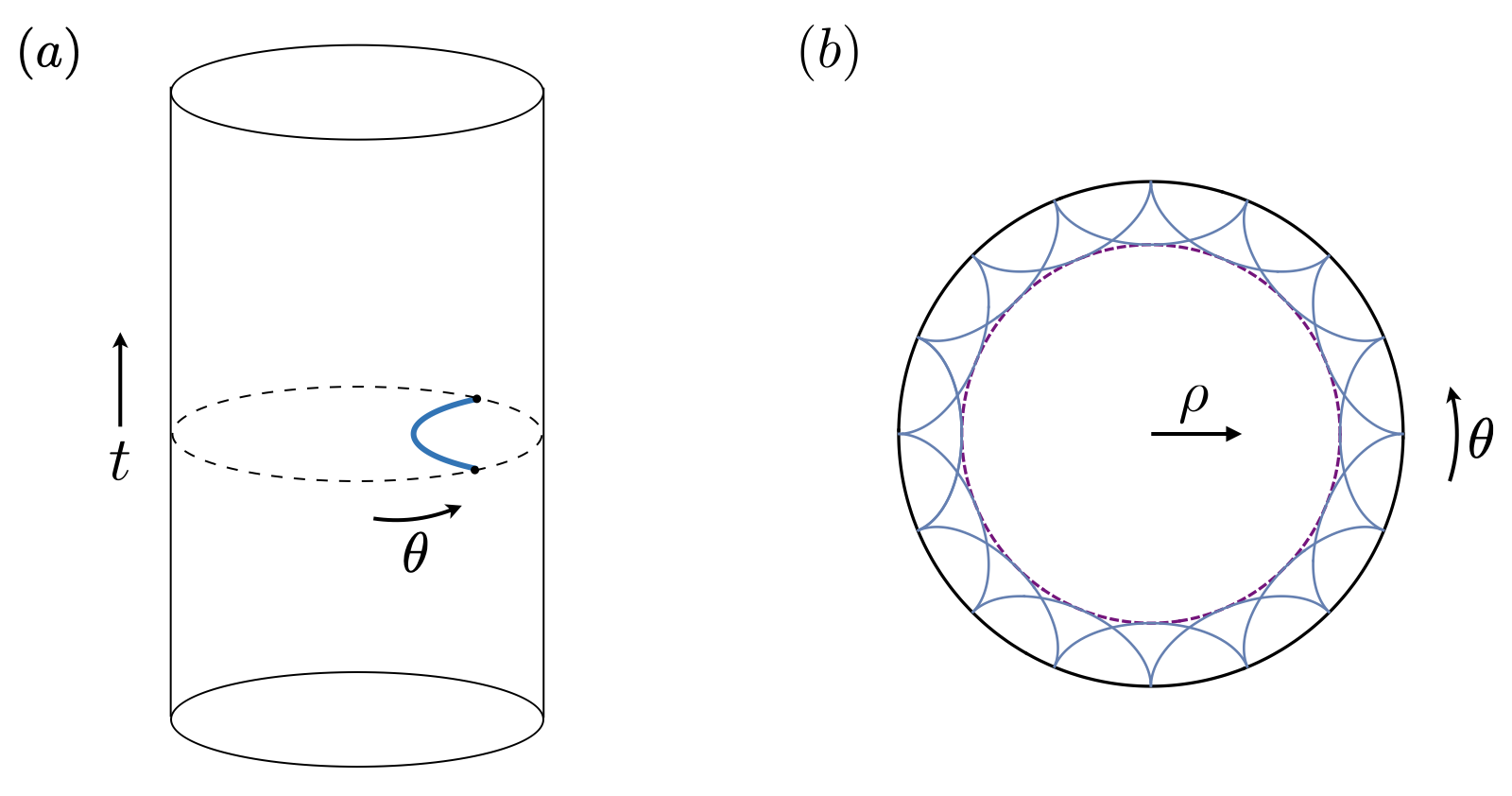
Another application arises in a subfield of holography known as ‘kinematic space,’ which studies the geometric properties of the space of spacelike pairs of points in a CFT_d and their role in probing the geometry of the bulk anti-de Sitter (AdS) spacetime Czech:2015qta; deBoer:2015kda; Czech:2016xec; deBoer:2016pqk. It was demonstrated that certain bilocal operators in a CFT pick up phases under a parallel transport that displaces the location of the spacelike points where they are evaluated. In the bulk AdS spacetime this was shown to compute the length of a curve traced out by geodesics limiting to these point pairs on the boundary (see Figure 1) Czech:2017zfq. As we show in Appendix A, these results for kinematic space can be understood using the language of state-based parallel transport.

Consider a subregion $A$ on a time slice of a CFT. Associated to this region is an algebra of operators $\mathcal{A}_{A}$. Assuming some short distance cutoff, the state is described by a reduced density matrix $\rho_{A}$, obtained from tracing the full state over the complement $\bar{A}$ of $A$. From this we can define the modular Hamiltonian $H_{\rm mod}$ through $\rho_{A}=e^{-H_{\rm mod}}/(\mbox{tr }e^{-H_{\rm mod}})$. The modular Hamiltonian encodes information about the entanglement properties of the state. It will be formally useful to refer to the ‘complete’ modular Hamiltonian $H_{\rm mod,A}-H_{\rm mod,\bar{A}}$. We will often drop the subscript $A$, and additionally allow the modular Hamiltonian to depend on some parameter $H_{\rm mod}(\lambda)$. This could for instance encode changes in the size of region $A$ as was studied in Czech:2017zfq; Czech:2019vih, or a change of state as we describe in the next section.

The physical data associated to $A$ is not the set of operators in $\mathcal{A}$, but rather their expectation values. As such, there can be symmetries, i.e, transformations which act on the algebra while leaving no imprint on measurable quantities. We define a modular zero mode $Q_{i}$ as a Hermitian operator that commutes with the modular Hamiltonian,

$$[Q_{i},H_{\rm mod}]=0~.$$

(5)

The modular zero mode can be exponentiated to the unitary

$$V=e^{-i\sum_{i}s_{i}Q_{i}}~.$$

(6)

Under the flow $\mathcal{O}\rightarrow V^{\dagger}\mathcal{O}V$, the expectation values of algebra elements are left unchanged while taking the algebra to itself. The transformation by modular zero modes therefore constitutes a kind of gauge redundancy.

Given an operator, it is often useful to separate the zero mode part out from a contribution that is non-ambiguous. In the finite-dimensional case, we can compute the zero mode contribution by using the projection operator

$$P_{0}[\mathcal{O}]=\sum_{E,q_{i},q_{i}^{\prime}}|E,q_{i}\rangle\langle E,q_{i}|\mathcal{O}|E,q_{i}^{\prime}\rangle\langle E,q_{i}^{\prime}|~,$$

(7)

where $|E,q_{i}\rangle$ are simultaneous eigenstates of $H_{\rm mod}$ and $Q_{i}$. Note that later we will be working with an infinite-dimensional algebra, where this formula no longer applies. We will show how to define an appropriate projection relevant for that situation in Section 3.

The zero mode frame redundancy leads to a Berry transport problem for operators. Imagine a process that modifies the algebra $\mathcal{A}_{A}$ depending on a parameter $\lambda$, for instance by changing the interval $A$ or the state. We start by diagonalizing the modular Hamiltonian,

$$H_{\rm mod}=U^{\dagger}\Delta U~,$$

(8)

where $\Delta$ is a diagonal matrix of eigenvalues. $H_{\rm mod},U$ and $\Delta$ are functions of $\lambda$ that vary along the path. Taking the derivative gives the ‘parallel transport equation,’

$$\dot{H}_{\rm mod}=[\dot{U}^{\dagger}U,H_{\rm mod}]+U^{\dagger}\dot{\Delta}U~,$$

(9)

where $\cdot=\partial_{\lambda}$. The first term on the right-hand side lies in the image of the adjoint action, $[\cdot,H_{\rm mod}].$ The second term encodes the change of spectrum under the parallel transport. It is a zero mode since it commutes with the modular Hamiltonian, in other words, it lies in the kernel of the adjoint action. We will assume that there is a unique decomposition into the image and kernel of the adjoint action, so that the entire zero mode contribution can be isolated from the second term: $P_{0}[\dot{H}_{\rm mod}]=U^{\dagger}\dot{\Delta}U$. For a discussion of subtleties associated with this assumption for the Virasoro algebra, see Appendix C.

This equation exhibits a redundancy due to the presence of modular zero modes. For instance, the modular Hamiltonian together with Eq. (9) could be equally well expressed in terms of $U\rightarrow\tilde{U}=UV$ where $V$ given by Eq. (6) is generated by a modular zero mode. Instead of Eq. (8) this gauge choice leads to

$$H_{\rm mod}=V^{\dagger}U^{\dagger}\Delta UV~.$$

(10)

A reasonable choice for fixing this ambiguity is to impose that

$$P_{0}[\partial_{\lambda}\tilde{U}^{\dagger}\tilde{U}]=0~.$$

(11)

Since $V$ preserves the zero mode space, $P_{0}[V^{\dagger}\dot{U}^{\dagger}UV]=V^{\dagger}P_{0}[\dot{U}^{\dagger}U]V$ from Eq. (7). Likewise, $\dot{V^{\dagger}}V$ is a modular zero mode from Eq. (6), so it projects to itself. Thus, this condition reduces to

$$-V^{\dagger}\dot{V}+V^{\dagger}P_{0}[\dot{U^{\dagger}}U]V=0~,$$

(12)

where we have used $\dot{V^{\dagger}}V=-V^{\dagger}\dot{V}$ since $V$ is unitary. We therefore obtain a more familiar expression for parallel transport of the operator $V$,

$$\left(\partial_{\lambda}-\Gamma\right)V=0~,$$

(13)

where

$$\Gamma=P_{0}[\dot{U^{\dagger}}U]$$

(14)

is a Berry connection that encodes information about how the zero mode frame changes as we vary the modular Hamiltonian. It transforms as $\Gamma\rightarrow V^{\dagger}\Gamma V-V^{\dagger}\dot{V}$ under $U\rightarrow UV$. After performing the parallel transport around a closed loop, $\dot{U}^{\dagger}U$ has a definite value by Eq. (11). However, $U$ itself may differ by a modular zero mode,

$$U(\lambda_{f})=U(\lambda_{i})e^{-i\sum_{i}\kappa_{i}Q_{i}}~.$$

(15)

Here, $\lambda_{f}=\lambda_{i}$ are the endpoints of a closed path. The coefficients $\kappa_{i}$ contain information about the loop.

There is also a curvature, $F$, associated to this parallel transport process. We can evaluate the curvature by performing parallel transport around a small loop. Here, ‘small’ means that we replace the derivatives with infinitesimal transformations. We can think of the operator $S_{\delta\lambda}=\tilde{U}^{\dagger}\delta_{\lambda}\tilde{U}$ as a generator of parallel transport. It transforms as a gauge field

$$S_{\delta\lambda}\to V^{\dagger}S_{\delta\lambda}V+V^{\dagger}\delta_{\lambda}V$$

(16)

under a change of modular frame $\tilde{U}\to\tilde{U}V$ and satisfies $P_{0}[S_{\delta\lambda}]=0$ by Eq. (11). The curvature $F$ associated to this gauge field is what we call the modular Berry curvature. It can be represented in the usual way by performing two consecutive infinitesimal transformations $\lambda_{i}\to\lambda_{i}+\delta_{1}\lambda$, followed by $\lambda_{i}+\delta_{1}\lambda\to\lambda_{i}+\delta_{1}\lambda+\delta_{2}\lambda$. Doing the same with $(1\leftrightarrow 2)$ and taking the difference gives a closed loop with

$$F=(1+S_{\delta_{2}\lambda}(\lambda_{i}+\delta_{1}\lambda))(1+S_{\delta_{1}\lambda}(\lambda_{i}))-(1\leftrightarrow 2)~.$$

(17)

Here, we use that the holonomy operator along the line $[\lambda_{i},\lambda_{i}+\delta\lambda]$ is given by

$$\exp\left(\int_{\lambda_{i}}^{\lambda_{i}+\delta\lambda}\tilde{U}^{\dagger}\delta_{\lambda}\tilde{U}\right)=1+S_{\delta\lambda}(\lambda_{i})~.$$

(18)

In Appendix B, we will derive a general expression for the curvature, Eq. (17), and we apply it in Section 3 to the case of state-changing parallel transport.

We now have all the ingredients to compute the curvature in an explicit example. We consider a general perturbation of the form

$\displaystyle z^{\prime}=z+\epsilon\,\xi(z)+\mathcal{O}(\epsilon^{2})~,$

(61)

where $\xi(z)$ is a wave packet

$$\xi(z)=\frac{1}{2\pi}\int_{-\infty}^{\infty}c(\lambda)\xi_{\lambda}(z)\,d\lambda~,$$

(62)

with $\xi_{\lambda}(z)$ defined in Eq. (43). We start by obtaining the correction to the transformed modular Hamiltonian upon acting with Eq. (61). Let us expand both the modular Hamiltonian and the parallel transport operator to first order in the small parameter $\epsilon$:

$$H^{\prime}_{\rm mod}=H^{(0)}+\epsilon\,H^{(1)}+\mathcal{O}(\epsilon^{2})~,\indent S=S^{(0)}+\epsilon\,S^{(1)}+\mathcal{O}(\epsilon^{2})~.$$

(63)

Using that $z=z^{\prime}-\epsilon\xi(z^{\prime})+\mathcal{O}(\epsilon^{2})$, one can expand the transformed $H_{\rm mod}$ to order $\mathcal{O}(\epsilon^{2})$. One finds that $H^{(0)}=H_{\rm mod}$ is the original modular Hamiltonian, while the correction is given by

$$H^{(1)}=-\frac{1}{2i}\oint\left[2z\xi(z)-(1+z^{2})\xi^{\prime}(z)\right]T(z)\,dz~.$$

(64)

Here, we have neglected the Schwarzian contribution for simplicity. It will be treated separately in Section 3.3. We now expand the parallel transport equation

$$\delta H_{\rm mod}=[S,H_{\rm mod}]$$

(65)

to first order in $\epsilon$. This gives two separate equations:

$$0=[S^{(0)},H^{(0)}]~,\quad H^{(1)}=[S^{(0)},H^{(1)}]+[S^{(1)},H^{(0)}]~.$$

(66)

Solving Eq. (66) for the correction $S^{(1)}$ to the parallel transport operator gives the solution

$$S^{(0)}=0~,\indent S^{(1)}=X_{\xi}~.$$

(67)

Both $S^{(0)}$ and $S^{(1)}$ are defined up to a zero mode, meaning that one can add to it an extra operator $Q$ for which $[Q,H_{\rm mod}]=0$ (e.g., the modular Hamiltonian itself) and the parallel transport equation would still be satisfied.

To compute the curvature we need to consider two different parallel transport operators $S_{1}$ and $S_{2}$ which we take to be defined according to the transformations

$$\xi_{1}(z)=\frac{1}{2\pi}\int_{-\infty}^{\infty}c_{1}(\lambda)\xi_{\lambda}(z)\,d\lambda~,\quad\xi_{2}(z)=\frac{1}{2\pi}\int_{-\infty}^{\infty}c_{2}(\lambda)\xi_{\lambda}(z)\,d\lambda~,$$

(68)

respectively. After projecting out their zero modes, we take the commutator and project to the zero modes again to obtain the value of the curvature component. Therefore, we need to compute

$$[S^{(1)}_{1}-\kappa_{1}H^{(0)},S^{(1)}_{2}-\kappa_{2}H^{(0)}]~,$$

(69)

where $\kappa_{i}=P_{0}(S_{i})$, is the zero mode coefficient of the parallel transport operator $S_{i}$. We can split Eq. (69) into terms that we can treat separately. Notice that the term proportional to $[H^{(0)},H^{(0)}]$ is zero and can be removed. Moreover, the definition of the projection operator immediately implies

$$P_{0}([S^{(1)}_{1},H^{(0)}])=P_{0}([S^{(1)}_{2},H^{(0)}])=0~.$$

(70)

To evaluate the last commutator we use the commutation relations in Eq. (45) to obtain

$$[S^{(1)}_{1},S^{(1)}_{2}]=\frac{1}{4\pi^{2}}\int_{-\infty}^{\infty}\int_{-\infty}^{\infty}(\lambda_{1}-\lambda_{2})c_{1}(\lambda_{1})c_{2}(\lambda_{2})X_{\lambda_{1}+\lambda_{2}}\,d\lambda_{1}d\lambda_{2}~.$$

(71)

Applying the projection operator sets $\lambda_{1}=-\lambda_{2}$, so that we find

$$P_{0}([S^{(1)}_{1},S^{(1)}_{2}])=2\int_{-\infty}^{\infty}\lambda\,c_{1}(\lambda)c_{2}(-\lambda)\,d\lambda~.$$

(72)

Therefore, the final result for the modular Berry curvature associated to the state-changing transport problem is given by

$$F=2\int_{-\infty}^{\infty}\lambda\,c_{1}(\lambda)c_{2}(-\lambda)\,d\lambda~.$$

(73)

Note that the curvature appropriately vanishes when two perturbations lie along the same direction, $c_{1}(\lambda)=c_{2}(\lambda)$. If we take the modes to be peaked at the eigenfunctions $\xi_{\lambda_{i}}(z)$ themselves, $c_{i}(\lambda)=\delta(\lambda-\lambda_{i})$, the above formula reduces to

$$F=(\lambda_{1}-\lambda_{2})\delta(\lambda_{1}+\lambda_{2})~,$$

(74)

which is a local formula in terms of the parameters $\lambda_{i}$.

To diagonalize the adjoint action, we saw that we must work with a continuous version of the Virasoro algebra. Viewed in terms of vector fields on the circle, we must consider non-smooth vector fields on the circle, Eq. (43), which have support only along the interval. When mapped to the real line, these are just plane waves, Eq. (54). In the last section, we performed parallel transport using wave packets constructed out of these eigenfunctions. In terms of the coordinates on the real line,

$$\xi(u)=\frac{1}{2\pi}\int_{-\infty}^{\infty}c(\lambda)\xi_{\lambda}(u)d\lambda~.$$

(75)

Now we would like to be more precise about the sense in which the corresponding vector fields form a Lie algebra. This amounts to imposing extra conditions on $c(\lambda)$ for these to form a closed algebra, along with any other desirable properties.

The simplest choice would be to demand that the $\xi(u)$ be smooth. Then, since the smoothness of functions is preserved under pointwise multiplication, the corresponding vector fields $\xi(u)\partial_{u}$ will form a closed algebra. However, an arbitrary $\xi(u)$ will not necessarily have finite zero mode projection, nor will there necessarily exist a natural definition for a dual space. To define sensible wave packets we will impose two additional requirements:

• •

  There is a notion of Fourier transform that maps the space to itself,

• •

  The $\xi(u)$ are integrable. This means that the projection, Eq. (58), is finite, and this property is preserved under commutation of the vector fields $\xi(u)\partial_{u}$ . It also allows us to define a dual space in terms of distributions.

To accomplish this, it is convenient to work with wave packets $\xi(u)$ that are Schwartz functions. These are smooth, bounded functions whose derivatives are also all bounded: $|u^{\alpha}\partial^{\beta}\xi(u)|<\infty$ for all $\alpha,\beta>0$. In other words, they rapidly go to zero as $u\rightarrow\pm\infty$, faster than any reciprocal power of $u$. This definition excludes for example polynomials, but includes polynomials weighted by an exponential $e^{-c|u|^{2}}$ for $c\in\mathbb{R}$. By the Leibniz rule, the Schwartz space $\mathcal{S}$ is closed under pointwise multiplication, thus the corresponding vector fields form a closed Lie algebra. We denote $\mathcal{S}$ for the space of Schwartz functions and $\mathfrak{s}$ for the corresponding algebra of vector fields.

Since these functions are integrable, it is natural to define a dual space $\mathcal{S}^{\prime}$ consisting of linear functionals $T:\mathcal{S}\rightarrow\mathbb{C}$, in terms of distributions:

$$T[\xi(u)]=\int_{-\infty}^{\infty}\xi(u)T(u)du~.$$

(76)

A pairing between Schwartz functions and dual elements can be defined from this as $\left<T,\xi\right>\equiv T[\xi(u)]$. Likewise, there is also a dual space $\mathfrak{s}^{*}$ consisting of linear functionals on $\mathfrak{s}$, the algebra of vector fields. This is inherited from the dual space $\mathcal{S}^{\prime}$, i.e., it consists of the space of distributions evaluated on Schwartz functions. There is a pairing $\left<\cdot,\cdot\right>$ between $\mathfrak{s}$ and $\mathfrak{s}^{*}$ which descends from the pairing on $\mathcal{S}$ and $\mathcal{S}^{\prime}$.

Notice that, evaluated on the wave packets Eq. (75), the projection operator Eq. (58)

$$P_{0}:\xi(u)\mapsto 2\pi c(0)~$$

(77)

is a linear functional, and thus it is an element of the dual space. The pairing is given by $\left<P_{0},\xi\right>=P_{0}(\xi)=2\pi c(0)$.

In the coordinates on the circle, recall that this dual element can be expressed from Eq. (59) as

$$P_{0}:\xi(z)\mapsto\frac{1}{\pi}\int dz\frac{\xi(z)}{(1+z^{2})^{2}}~.$$

(78)

Notice that this dual element is not a smooth quadratic form on the circle as is typically considered in treatments of the dual space of the Virasoro algebra, but rather a more general distribution that involves singularities at $z=\pm i$⁶⁶ 6 In the usual discussion of the Virasoro algebra the dual space is identified with the space of smooth quadratic differentials. Formally, one could argue that distributions such as $\delta(z-z_{0})$ and $\delta^{\prime}(z-z_{0})$ are also part of some suitably defined notion of the dual space. Indeed, they define linear functionals $$\xi\mapsto\xi(z_{0})~,\hskip 10.0pt\xi\mapsto-\xi^{\prime}(z_{0})~,$$ (79) which evaluate a function (or its derivative) at some point $z_{0}$. The projection operator $P_{0}$ in Eq. (78), when integrated over the full circle and properly regularized, can be regarded in this fashion. See Appendix C for more details, for example, Eqs. (208) - (210).. A standard definition of the dual space is an attempt to get a space that is roughly the same size as the algebra itself. For infinite-dimensional spaces the formal dual is much larger and one needs some additional structure, e.g., that of a Hilbert space, to limit it.

We emphasize that there is considerable freedom in these definitions. A different choice would amount to taking a different set-up for varying the state in the parallel transport process. Our definitions allow us to perform parallel transport using wavefunctions that are ‘physical’ in the sense of being Fourier transformable and integrable. The existence of a natural dual space also allows for contact with a geometrical picture in terms of coadjoint orbits, which we describe in the next section.

We have so far only considered changing the state with a transformation of the circle. When the transformations are diffeomorphisms on the circle, the group $\rm{Diff}(S^{1})$ gets centrally extended to the full Virasoro group, $\rm{Diff}(S^{1})\times\mathbb{R}$. Here we are considering a continuous version of the Virasoro generated by the transformations, Eq. (43). For the central extension, we proceed in direct analogy with the Virasoro case. In the following, the vector fields $\xi(z)$ should be understood to have non-zero support only between $z=\pm i$, so that this is the only part of the integral over the full circle that contributes.

We consider pairs $(\xi,\alpha)$, where $\xi$ is a vector field of the form Eq. (43), which diagonalizes the adjoint action, and $\alpha\in\mathbb{R}$. The Lie bracket is defined as

$$\left[(\xi,\alpha),(\chi,\beta)\right]=\left(-[\xi,\chi],-\frac{1}{48\pi}\oint dz\,(\xi(z)\chi^{\prime\prime\prime}(z)-\xi^{\prime\prime\prime}(z)\chi(z))\right)~,$$

(80)

where $[\xi,\chi]:=\xi\chi^{\prime}-\chi\xi^{\prime}$ is the commutator of vector fields. This is identical to the commutators for the Virasoro algebra, with the only difference being that we integrate only over half the circle, and also consider transformations $\xi$ which are not smooth at the endpoints. In terms of the operators $X_{\lambda}$, this extends the algebra in Eq. (45) to

$$[\bar{X}_{\bar{\lambda}},\bar{X}_{\bar{\mu}}]=(\bar{\lambda}-\bar{\mu})\bar{X}_{\bar{\lambda}+\bar{\mu}}+\frac{c}{12}\bar{\lambda}(\bar{\lambda}^{2}+1)\delta(\bar{\lambda}+\bar{\mu})~.$$

(81)

where we have defined rescaled barred variables through $X_{\lambda}=-2\pi\bar{X}_{\lambda},\lambda=-2\pi\bar{\lambda}$ to bring this to a form that more closely resembles the usual Virasoro algebra with discrete labels.

One often introduces a new generator, denoted by $c$, which commutes with all other elements in the algebra, to write

$$(\xi,\alpha)=\xi(z)\partial_{z}-i\alpha c~.$$

(82)

By definition, the central element $c$ commutes with $H_{\rm mod}$, i.e., $[H_{\rm mod},c]=0$. Therefore, we can think about the central element as another zero mode in the parallel transport problem.

Luckily, the situation for the central element is simpler than for the modular Hamiltonian itself. From the form of $H_{\rm mod}$, Eq. (37), and the algebra, Eq. (80), we see that the central element $c$ does not appear in commutators of the form $[H_{\rm mod},X]$. Therefore, the projection onto the coefficient of $c$ is simply given by the linear functional

$$(\xi,\alpha)\to\alpha~.$$

(83)

One way to include the information of the central term is to make the Berry curvature give a $U(1)\times U(1)$-valued number (organized in terms of an extra element which we take to be $c$). More precisely, we define the zero mode projection operator $P^{c}_{0}$, which depends on $c$, by

$$P^{c}_{0}((X_{\xi},\alpha))=P_{0}(X_{\xi})-\alpha c~.$$

(84)

The first term is the usual zero mode, while the second term keeps track of the central zero mode. It is easy to see how the result for the Berry curvature gets modified. Using Eq. (28) with $P_{0}^{c}$ instead of $P_{0}$, we see that the formula for the Berry curvature is given by

$$F=P_{0}([X_{\xi_{1}},X_{\xi_{2}}])+\frac{c}{48\pi}\oint dz\,\left(\xi_{1}(z)\xi_{2}^{\prime\prime\prime}(z)-\xi_{1}^{\prime\prime\prime}(z)\xi_{2}(z)\right)~.$$

(85)

As a consistency check, we can go back to our example in Section 3.1 and consider the contribution from the Schwarzian term in Eq. (64). Expanding the parallel transport equation, we need to solve

$$H^{(1)}=[S^{(1)},H^{(0)}]~,$$

(86)

where the change in the modular Hamiltonian due to the Schwarzian derivative to first order is given by

$$H^{(1)}_{\rm Schw}=\frac{c}{24i}\oint dz(1+z^{2})\xi^{\prime\prime\prime}(z)~,$$

(87)

having used that $\{z^{\prime},z\}=\epsilon\xi^{\prime\prime\prime}+{\cal{O}}(\epsilon^{2})$. On the full circle, applying three integration by parts, this is just $H^{(1)}_{\rm Schw}=0$ (equivalently, no diffeomorphism has $\xi^{\prime\prime\prime}=z^{-1}$ or $z^{-3}$ which would give a pole). The situation is a bit more subtle on the half circle, since due to non-differentiability at the endpoints it is no longer valid to apply integration by parts multiple times. However, it is still the case that none of the eigenfunctions, Eq. (43), have $\xi^{\prime\prime\prime}=z^{-1}$ or $z^{-3}$, and so the Schwarzian contribution vanishes. Thus, in either case the solution to Eq. (86) with the new Lie bracket Eq. (80) is still given by $S^{(1)}=X_{\xi}~$. The extra contribution to the commutator $[S^{(1)}_{1},S^{(1)}_{2}]$ due to the central charge is indeed given by Eq. (85).

References

- (1) B. Czech, L. Lamprou, S. McCandlish, B. Mosk and J. Sully, A Stereoscopic Look into the Bulk, JHEP 07 (2016) 129 [1604.03110].
- (2) J. de Boer, F.M. Haehl, M.P. Heller and R.C. Myers, Entanglement, holography and causal diamonds, JHEP 08 (2016) 162 [1606.03307].
- (3) J. de Boer, M.P. Heller, R.C. Myers and Y. Neiman, Holographic de Sitter Geometry from Entanglement in Conformal Field Theory, Phys. Rev. Lett. 116 (2016) 061602 [1509.00113].
- (4) B. Czech, L. Lamprou, S. McCandlish and J. Sully, Integral Geometry and Holography, JHEP 10 (2015) 175 [1505.05515].
- (5) C.T. Asplund, N. Callebaut and C. Zukowski, Equivalence of Emergent de Sitter Spaces from Conformal Field Theory, JHEP 09 (2016) 154 [1604.02687].
- (6) B. Freivogel, R. Jefferson, L. Kabir, B. Mosk and I.-S. Yang, Casting Shadows on Holographic Reconstruction, Phys. Rev. D 91 (2015) 086013 [1412.5175].
- (7) R. Espíndola, A. Guijosa and J.F. Pedraza, Entanglement Wedge Reconstruction and Entanglement of Purification, Eur. Phys. J. C 78 (2018) 646 [1804.05855].
- (8) R.F. Penna and C. Zukowski, Kinematic space and the orbit method, JHEP 07 (2019) 045 [1812.02176].
- (9) B. Czech, L. Lamprou, S. Mccandlish and J. Sully, Modular Berry Connection for Entangled Subregions in AdS/CFT, Phys. Rev. Lett. 120 (2018) 091601 [1712.07123].
- (10) B. Czech, J. De Boer, D. Ge and L. Lamprou, A modular sewing kit for entanglement wedges, JHEP 11 (2019) 094 [1903.04493].
- (11) J. Maldacena, D. Simmons-Duffin and A. Zhiboedov, Looking for a bulk point, JHEP 01 (2017) 013 [1509.03612].
- (12) N. Engelhardt and G.T. Horowitz, Towards a Reconstruction of General Bulk Metrics, Class. Quant. Grav. 34 (2017) 015004 [1605.01070].
- (13) N. Engelhardt and G.T. Horowitz, Recovering the spacetime metric from a holographic dual, Adv. Theor. Math. Phys. 21 (2017) 1635 [1612.00391].
- (14) N. Engelhardt and A.C. Wall, Extremal Surface Barriers, JHEP 03 (2014) 068 [1312.3699].
- (15) N. Chagnet, S. Chapman, J. de Boer and C. Zukowski, Complexity for Conformal Field Theories in General Dimensions, 2103.06920.
- (16) J. Maldacena and L. Susskind, Cool horizons for entangled black holes, Fortsch. Phys. 61 (2013) 781 [1306.0533].
- (17) J. De Boer and L. Lamprou, Holographic Order from Modular Chaos, JHEP 06 (2020) 024 [1912.02810].
- (18) J. Kirklin, The Holographic Dual of the Entanglement Wedge Symplectic Form, JHEP 01 (2020) 071 [1910.00457].
- (19) H. Casini, M. Huerta and R.C. Myers, Towards a derivation of holographic entanglement entropy, JHEP 05 (2011) 036 [1102.0440].
- (20) B. Oblak, Berry Phases on Virasoro Orbits, JHEP 10 (2017) 114 [1703.06142].
- (21) A.M. Perelomov, Generalized coherent states and their applications (1986).
- (22) L.G. Yaffe, Large n Limits as Classical Mechanics, Rev. Mod. Phys. 54 (1982) 407.
- (23) P. Caputa and J.M. Magan, Quantum Computation as Gravity, Phys. Rev. Lett. 122 (2019) 231302 [1807.04422].
- (24) P. Bueno, J.M. Magan and C.S. Shahbazi, Complexity measures in QFT and constrained geometric actions, 1908.03577.
- (25) I. Akal, Reflections on Virasoro circuit complexity and Berry phase, 1908.08514.
- (26) J. Erdmenger, M. Gerbershagen and A.-L. Weigel, Complexity measures from geometric actions on Virasoro and Kac-Moody orbits, JHEP 11 (2020) 003 [2004.03619].
- (27) M. Flory and M.P. Heller, Geometry of Complexity in Conformal Field Theory, Phys. Rev. Res. 2 (2020) 043438 [2005.02415].
- (28) M. Flory and M.P. Heller, Conformal field theory complexity from Euler-Arnold equations, JHEP 12 (2020) 091 [2007.11555].
- (29) P. Caputa, J.M. Magan and D. Patramanis, Geometry of Krylov Complexity, 2109.03824.
- (30) D. Patramanis, Probing the entanglement of operator growth, 2111.03424.
- (31) J. Cardy and E. Tonni, Entanglement hamiltonians in two-dimensional conformal field theory, J. Stat. Mech. 1612 (2016) 123103 [1608.01283].
- (32) D.D. Blanco, H. Casini, L.-Y. Hung and R.C. Myers, Relative Entropy and Holography, JHEP 08 (2013) 060 [1305.3182].
- (33) S. Das, B. Ezhuthachan, S. Porey and B. Roy, Virasoro algebras, kinematic space and the spectrum of modular Hamiltonians in CFT2, JHEP 21 (2020) 123 [2101.10211].
- (34) N. Ishibashi and T. Tada, Infinite circumference limit of conformal field theory, J. Phys. A 48 (2015) 315402 [1504.00138].
- (35) N. Ishibashi and T. Tada, Dipolar quantization and the infinite circumference limit of two-dimensional conformal field theories, Int. J. Mod. Phys. A 31 (2016) 1650170 [1602.01190].
- (36) A. Gendiar, R. Krcmar and T. Nishino, Spherical Deformation for One-Dimensional Quantum Systems, Prog. Theor. Phys. 122 (2009) 953 [0810.0622].
- (37) H. Katsura, Sine-square deformation of solvable spin chains and conformal field theories, J. Phys. A 45 (2012) 115003 [1110.2459].
- (38) B. Doyon, M. Hoogeveen and D. Bernard, Energy flow and fluctuations in non-equilibrium conformal field theory on star graphs, J. Stat. Mech. 1403 (2014) P03002 [1306.3192].
- (39) E. Witten, Coadjoint Orbits of the Virasoro Group, Commun. Math. Phys. 114 (1988) 1.
- (40) A. Alekseev and S.L. Shatashvili, Path Integral Quantization of the Coadjoint Orbits of the Virasoro Group and 2D Gravity, Nucl. Phys. B 323 (1989) 719.
- (41) A. Kirillov, Lectures on the Orbit Method, vol. 64 of Graduate Studies in Mathematics, American Mathematical Society (July, 2004), http://dx.doi.org/10.1090/gsm/064.
- (42) A. Alekseev and S.L. Shatashvili, Coadjoint Orbits, Cocycles and Gravitational Wess–Zumino, Rev. Math. Phys. 30 (2018) 1840001 [1801.07963].
- (43) A. Belin, A. Lewkowycz and G. Sárosi, The boundary dual of the bulk symplectic form, Phys. Lett. B 789 (2019) 71 [1806.10144].
- (44) A. Belin, A. Lewkowycz and G. Sárosi, Complexity and the bulk volume, a new York time story, JHEP 03 (2019) 044 [1811.03097].
- (45) D. Marolf, O. Parrikar, C. Rabideau, A. Izadi Rad and M. Van Raamsdonk, From Euclidean Sources to Lorentzian Spacetimes in Holographic Conformal Field Theories, JHEP 06 (2018) 077 [1709.10101].
- (46) A. Lewkowycz and J. Maldacena, Generalized gravitational entropy, JHEP 08 (2013) 090 [1304.4926].
- (47) X. Dong, The Gravity Dual of Renyi Entropy, Nature Commun. 7 (2016) 12472 [1601.06788].
- (48) X. Dong, Holographic Entanglement Entropy for General Higher Derivative Gravity, JHEP 01 (2014) 044 [1310.5713].
- (49) L.-Y. Hung, R.C. Myers, M. Smolkin and A. Yale, Holographic Calculations of Renyi Entropy, JHEP 12 (2011) 047 [1110.1084].
- (50) K. Krasnov, On holomorphic factorization in asymptotically AdS 3-D gravity, Class. Quant. Grav. 20 (2003) 4015 [hep-th/0109198].
- (51) P. Calabrese and J.L. Cardy, Entanglement entropy and quantum field theory, J. Stat. Mech. 0406 (2004) P06002 [hep-th/0405152].
- (52) M. Banados, Three-dimensional quantum geometry and black holes, AIP Conf. Proc. 484 (1999) 147 [hep-th/9901148].
- (53) E. Witten, Quantization of Chern-Simons gauge theory with complex gauge group, Communications in Mathematical Physics 137 (1991) 29 .
- (54) J. Cotler and K. Jensen, A theory of reparameterizations for AdS3 gravity, JHEP 02 (2019) 079 [1808.03263].
- (55) G. Barnich, H.A. Gonzalez and P. Salgado-Rebolledo, Geometric actions for three-dimensional gravity, Class. Quant. Grav. 35 (2018) 014003 [1707.08887].
- (56) O. Coussaert, M. Henneaux and P. van Driel, The Asymptotic dynamics of three-dimensional Einstein gravity with a negative cosmological constant, Class. Quant. Grav. 12 (1995) 2961 [gr-qc/9506019].
- (57) P. Kraus, R. Monten and R.M. Myers, 3D Gravity in a Box, 2103.13398.
- (58) W. Donnelly and L. Freidel, Local subsystems in gauge theory and gravity, JHEP 09 (2016) 102 [1601.04744].
- (59) A.J. Speranza, Local phase space and edge modes for diffeomorphism-invariant theories, JHEP 02 (2018) 021 [1706.05061].
- (60) W. Donnelly, L. Freidel, S.F. Moosavian and A.J. Speranza, Gravitational edge modes, coadjoint orbits, and hydrodynamics, JHEP 09 (2021) 008 [2012.10367].
- (61) T. Faulkner, R.G. Leigh and O. Parrikar, Shape Dependence of Entanglement Entropy in Conformal Field Theories, JHEP 04 (2016) 088 [1511.05179].
- (62) T. Faulkner, R.G. Leigh, O. Parrikar and H. Wang, Modular Hamiltonians for Deformed Half-Spaces and the Averaged Null Energy Condition, JHEP 09 (2016) 038 [1605.08072].
- (63) A. Lewkowycz and O. Parrikar, The holographic shape of entanglement and Einstein’s equations, JHEP 05 (2018) 147 [1802.10103].
- (64) S. Banerjee, Wess-Zumino Consistency Condition for Entanglement Entropy, Phys. Rev. Lett. 109 (2012) 010402 [1109.5672].
- (65) P. Caputa and S. Datta, Operator growth in 2d CFT, 2110.10519.