跳到论文正文
W Papers独立论文阅读器 arXiv:2111.05210 论文正文 计算阅读时间 · 0%
引用这篇论文根据当前论文元数据生成,正式投稿前建议核对。


License: arXiv.org perpetual non-exclusive license
arXiv:2111.05210v1 [math.NA] 09 Nov 2021

An F-modulated stability framework for multistep methods

Dong Li Address: D. Li, SUSTech International Center for Mathematics, and Department of Mathematics, Southern University of Science and Technology, Shenzhen, China 518055, PRC Email address: lid@sustech.edu.cn , Chaoyu Quan Address: C.Y. Quan, SUSTech International Center for Mathematics, and Department of Mathematics, Southern University of Science and Technology, Shenzhen, P.R. China Email address: quancy@sustech.edu.cn and Wen Yang Address: W. Yang, Wuhan Institute of Physics and Mathematics, Innovation Academy for Precision Measurement Science and Technology, Chinese Academy of Sciences, Wuhan 430071, P. R. China. Email address: wyang@wipm.ac.cn
Abstract.

We introduce a new 𝐅\mathbf{F}-modulated energy stability framework for general linear multistep methods. We showcase the theory for the two dimensional molecular beam epitaxy model with no slope selection which is a prototypical gradient flow with Lipschitz-bounded nonlinearity. We employ a class of representative BDFkk, 2≤k≤52\leq k\leq 5 discretization schemes with explicit kthk^{\mathrm{th}}-order extrapolation of the nonlinear term. We prove the uniform-in-time boundedness of high Sobolev norms of the numerical solution. The upper bound is unconditional, i.e. regardless of the size of the time step. We develop a new algebraic theory and calibrate nearly optimal and explicit maximal time step constraints which guarantee monotonic 𝐅\mathbf{F}-modulated energy dissipation.

1. Introduction

Phase field models such as the Allen–Cahn (AC) equations [3], the Cahn–Hilliard (CH) equations [4], and the molecular beam epitaxy (MBE) models [6] have been widely used in material sciences, multiphase flow, biology, image processing and the like. In this work for convenience of presentation we consider a prototypical MBE model with no slope selection (MBE-NSS) posed on the two-dimensional periodic torus Ω=𝕋2=[−π,π]2\Omega=\mathbb{T}^{2}=[-\pi,\pi]^{2}:

∂tu=−ν​Δ2​u−∇⋅(f⁡(∇u)),(t,x)∈(0,∞)×Ω,\displaystyle\partial_{t}u=-\nu\Delta^{2}u-\nabla\cdot\Bigl(f(\nabla u)\Bigr),\qquad(t,x)\in(0,\infty)\times\Omega, (1.1)

where f⁡(z)=z1+|z|2f(z)=\frac{z}{1+|z|^{2}}, and |z|=z12+z22|z|=\sqrt{z_{1}^{2}+z_{2}^{2}} for z=(z1,z2)T∈ℝ2z=(z_{1},z_{2})^{\mathrm{T}}\in\mathbb{R}^{2}. The real-valued function u=u⁡(t,x)u=u(t,x) is called a scaled height function of the thin film in a co-moving frame. The linear dissipative term −ν​Δ2​u-\nu\Delta^{2}u represents to capillarity-driven isotropic surface diffusion (cf. Mullins [21] and Herring [22]) with ν>0\nu>0 being the diffusion coefficient. The dynamical evolution (1.1) can be derived from the L2L^{2} gradient flow of the energy functional

ℰ⁡(u)=∫Ω(−12​log⁡(1+|∇u|2)+12​ν​|Δ​u|2)​𝑑x.\displaystyle\mathcal{E}(u)=\int_{\Omega}\Bigl(-\frac{1}{2}\log(1+|\nabla u|^{2})+\frac{1}{2}\nu|\Delta u|^{2}\Bigr)dx. (1.2)

One should note that the sign in front of the logarithmic potential is negative which is a manifestation of the Ehrlich-Schwoebel effect. Due to the strong competition between the potential term and the biharmonic diffusion term, an uphill atom current is often generated in the system which leads to mound-like structures in the film. Under the assumption |∇u|≪1|\nabla u|\ll 1, the energy functional (1.2) can be roughly approximated by a simpler-looking functional

ℰSS​(u)=∫Ω(14​(|∇u|2−1)2+12​η2​|Δ​u|2)​𝑑x.\displaystyle\mathcal{E}^{\mathrm{SS}}(u)=\int_{\Omega}\Bigl(\frac{1}{4}(|\nabla u|^{2}-1)^{2}+\frac{1}{2}\eta^{2}|\Delta u|^{2}\Bigr)dx. (1.3)

The L2L^{2}-gradient flow of ℰSS\mathcal{E}^{\mathrm{SS}} corresponds to the MBE model with slope-selection, i.e. the system typically favors the slope |∇u|≈1|\nabla u|\approx 1 which exhibits pyramidal structures. In stark contrast prototypical solutions to (1.1) have mound-like structures whose slopes can have a large upper bound. On the other hand from the analysis point of view, the system (1.1) is more benign than (1.3) since the nonlinear term has bounded derivatives of all orders. This is of fundamental importance since it leads to strong a priori bound of the PDE solution uniformly in time. For smooth solutions to (1.1), the mean-value of uu is preserved in time. For simplicity we set this mean value to be zero throughout this work. The fundamental energy conservation law takes the form

ℰ⁡(u⁡(t2))+∫t1t2‖∂tu‖22​𝑑t=ℰ⁡(u⁡(t1)),∀ 0≤t1<t2<∞.\displaystyle\mathcal{E}(u(t_{2}))+\int_{t_{1}}^{t_{2}}\|\partial_{t}u\|_{2}^{2}dt=\mathcal{E}(u(t_{1})),\qquad\forall\,0\leq t_{1}<t_{2}<\infty. (1.4)

This yields

ℰ⁡(u⁡(t2))≤ℰ⁡(u⁡(t1)),∀t2≥t1.\displaystyle\mathcal{E}(u(t_{2}))\leq\mathcal{E}(u(t_{1})),\qquad\forall\,t_{2}\geq t_{1}. (1.5)

Since the mean value of uu is zero and the energy is coercive, the estimate (1.5) gives a priori global H2H^{2} control of the solution. The wellposedness and regularity of solutions to (1.1) follows easily from this and the fact that the nonlinear term has bounded derivatives of all orders.

In the study of phase field models a fundamental problem is to design efficient, accurate and stable numerical schemes which can accommodate vastly different spatial and temporal scales. A sampler of existing popular numerical methods includes the convex-splitting scheme [5, 7, 19], the stabilization scheme [18, 20], the scalar auxiliary variable (SAV) scheme [17], semi-implicit/implicit-explicit (IMEX) schemes [10, 12, 11] and so on. Recently a new theoretical framework has been established ([10, 12, 11]) to analyze the stability and convergence of typical semi-implicit methods of order up to two. However due to the lack of monotonic discrete energy law there are very few works in the literature devoted to the analysis of stability of higher order methods. In practical numerical implementations it is often observed that the energy of higher order methods typically exhibits sporadic non-monotonic oscillations for medium time step sizes. As such it was already realized and heuristically argued in [20] that high order methods should dissipate a suitably modified energy functional ℰΔ​t\mathcal{E}_{\Delta t} which differs from the standard energy by a minuscule O⁡(Δ​tp)O(\Delta t^{p}) correction. In [9], by an ingenious cut-off procedure which caps the numerical solution with the PDE maximum principle, Li, Yang and Zhou proved rigorously the L2L^{2} stability of a class of high order methods for parabolic equations. Concerning the molecular beam epitaxy model with no slope selection, Hao, Huang and Wang [8] recently proposed a BDF3/AB3 scheme with a judiciously chosen additional stabilization term of the form −A​Δ​t2​Δ2​(un+1−un)-A\Delta t^{2}\Delta^{2}(u^{n+1}-u^{n}). It was rigorously shown in [8] that if A≥O⁡(ν−1)A\geq O(\nu^{-1}) then one can achieve unconditional energy stability regardless of the size of the time step. In recent [13], a BDF3/EP3 semi-discretization scheme was analyzed for the MBE model with no slope selection. Explicit and nearly optimal time step constraints were identified in [13] for which the modified energy dissipation law is rigorously proved to hold. Moreover an unconditional uniform energy bound was proved in [13] with no size restrictions on the time step. However, whilst the analysis framework in [13] is quite satisfactory for the BDFk methods of order less than three, it is by no means trivial to extend it to higher order methods such as BDFk, k≥3k\geq 3. The purpose of this work is to develop further the program initiated in [10, 12, 11, 13] and construct a new 𝐅\mathbf{F}-modulated energy stability framework for general linear multistep methods.

To this end we first review the situation with general BDFkk schemes applied on linear models. A general qq-step method (cf. page 21 of [1]) for the ODE y′=f⁡(y)y^{\prime}=f(y) takes the form ∑j=0qaj​yn+j=τ​∑j=0qbj​f​(yn+j).\sum_{j=0}^{q}a_{j}y^{n+j}=\tau\sum_{j=0}^{q}b_{j}f(y^{n+j}). A method is of order q≥1q\geq 1 iff. ∑j=0qaj​y​((n+j)​τ)−τ​∑j=0qbj​f​(y⁡((n+j)​τ))=𝒪⁡(τq+1)\sum_{j=0}^{q}a_{j}y((n+j)\tau)-\tau\sum_{j=0}^{q}b_{j}f(y((n+j)\tau))=\mathcal{O}(\tau^{q+1}) for all sufficiently smooth yy and the rate 𝒪⁡(τq+1)\mathcal{O}(\tau^{q+1}) cannot be improved for some specific yy. In terms of the polynomials ρ⁡(w)=∑j=0qaj​wj\rho(w)=\sum_{j=0}^{q}a_{j}w^{j}, σ⁡(w)=∑j=0qbj​wj\sigma(w)=\sum_{j=0}^{q}b_{j}w^{j}, this amounts to requiring for some c≠0c\neq 0,

ρ⁡(w)−σ⁡(w)​ln⁡w=c​(w−1)q+1+𝒪⁡(|w−1|q+2).\displaystyle\rho(w)-\sigma(w)\ln w=c(w-1)^{q+1}+\mathcal{O}(|w-1|^{q+2}). (1.6)

A BDFqq method corresponds to specifying σ⁡(w)=(∑j=1q1j)​wq\sigma(w)=(\sum_{j=1}^{q}\frac{1}{j})w^{q} and ρ⁡(w)=∑j=1q1j​ξq−j​(ξ−1)j\rho(w)=\sum_{j=1}^{q}\frac{1}{j}\xi^{q-j}(\xi-1)^{j}. In the literature one usually considers the general Banach space ODE:

u′+A​u=0,0<t<T,\displaystyle u^{\prime}+Au=0,\quad 0<t<T, (1.7)

where AA is a positive definite, self-adjoint, linear operator on a Hilbert space HH with dense domain D⁡(A)D(A). A qq-step BDF method typically takes the form

∑j=0qajun+j+τAun+q=0,n=0,⋯,N−q,\displaystyle\sum_{j=0}^{q}a_{j}u^{n+j}+\tau Au^{n+q}=0,\qquad n=0,\cdots,N-q, (1.8)

where the coefficients aja_{j} are extracted from the polynomial ρ⁡(w)=∑j=1q1j​ξq−j​(ξ−1)j=∑j=0qaj​ξj\rho(w)=\sum_{j=1}^{q}\frac{1}{j}\xi^{q-j}(\xi-1)^{j}=\sum_{j=0}^{q}a_{j}\xi^{j}. To make the energy method applicable to the parabolic equations, Nevanlinnna and Odeh [16] introduced multipliers for BDFkk methods with 3≤k≤53\leq k\leq 5. See also Lubich, Mansour and Venkataraman [15] for a powerful application in the stability analysis of parabolic equations. In recent [2], Akrivis, Chen, Yu and Zhou showed boundedness for the heat equation by using a novel multiplier for the BDF6 method. In the same work it was also shown that no Nevanlinna-Odeh multiplier exists. However, at present it is unknown whether these multiplier techniques can be used in the nonlinear situations due to subtle technical obstructions.

In this work we propose a new theoretical framework for establishing the energy stability of extrapolated BDFkk schemes for general gradient flows with Lipschitz nonlinearities. To showcase our analysis we consider the model case MBE equations with no slope selection. We shall not rely on any existing multiplier techniques, but will develop a completely new 𝐅\mathbf{F}-modulated energy stability framework which guarantees the energy dissipation with a very mild restriction on the time step (cf. Table 1). One should note that in Table 1, the explicit time step constraints are (as far as we know) the first of the kind in the literature which accords very well with what is observed in practical numerical implementations.

Table 1. Optimal time step τmax\tau_{\max} for 𝐅\mathbf{F}-modulated energy dissipation.
 
BDF2 BDF33 BDF44 BDF55
τmax\tau_{\mathrm{max}} 1.771626​ν1.771626\nu 0.211023​ν0.211023\nu 0.032644​ν0.032644\nu 0.001635​ν0.001635\nu
 

In the second part of our work, by another novel analysis we show that the energy of BDFkk with 2≤k≤52\leq k\leq 5 remains uniformly bounded in H2H^{2} which is also unconditional, i.e. regardless of the size of the time step.

The rest of this paper is organized as follows. In Section 2, we introduce the 𝐅\mathbf{F}-modulated energy for the BDFkk/EPkk scheme of the MBE-NSS equation and identify the explicit time step constraints for energy dissipation. In Section 3 we prove uniform energy boundedness of the numerical iterates with no restrictions on the size of the time step.

2. Energy dissipation of general BDFkk schemes

Classical BDFkk schemes for ODE y′=f⁡(y)y^{\prime}=f(y) takes the form (see [14, pp. 173])

BDF1:yn+1−yn=τ​f​(yn+1)(backward​Euler);\displaystyle\mathrm{BDF1:~}y^{n+1}-y^{n}=\tau f(y^{n+1})\quad(\mathrm{backward~Euler});
BDF2:32​yn+2−2​yn+1+12​yn=τ​f​(yn+2);\displaystyle\mathrm{BDF2:~}\tfrac{3}{2}y^{n+2}-2y^{n+1}+\tfrac{1}{2}y^{n}=\tau f(y^{n+2});
BDF3:116​yn+3−3​yn+2+32​yn+1−13​yn=τ​f​(yn+3);\displaystyle\mathrm{BDF3:~}\tfrac{11}{6}y^{n+3}-3y^{n+2}+\tfrac{3}{2}y^{n+1}-\tfrac{1}{3}y^{n}=\tau f(y^{n+3});
BDF4:2512​yn+4−4​yn+3+3​yn+2−43​yn+1+14​yn=τ​f​(yn+4);\displaystyle\mathrm{BDF4:~}\tfrac{25}{12}y^{n+4}-4y^{n+3}+3y^{n+2}-\tfrac{4}{3}y^{n+1}+\tfrac{1}{4}y^{n}=\tau f(y^{n+4});
BDF5:13760​yn+5−5​yn+4+5​yn+3−103​yn+2+54​yn+1−15​yn=τ​f​(yn+5);\displaystyle\mathrm{BDF5:~}\tfrac{137}{60}y^{n+5}-5y^{n+4}+5y^{n+3}-\tfrac{10}{3}y^{n+2}+\tfrac{5}{4}y^{n+1}-\tfrac{1}{5}y^{n}=\tau f(y^{n+5});
BDF6:4920​yn+6−6​yn+5+152​yn+4−203​yn+3+154​yn+2−65​yn+1+16​yn=τ​f​(yn+6).\displaystyle\mathrm{BDF6:~}\tfrac{49}{20}y^{n+6}-6y^{n+5}+\tfrac{15}{2}y^{n+4}-\tfrac{20}{3}y^{n+3}+\tfrac{15}{4}y^{n+2}-\tfrac{6}{5}y^{n+1}+\tfrac{1}{6}y^{n}=\tau f(y^{n+6}).

Methods with k>6k>6 are not zero-stable so they cannot be used. For a fixed BDFkk method, the LHS of the above can be rewritten as

∑i=0kAi(k)​yn+k−i=∑i=0k−1ai(k)​(yn+k−i−yn+k−i−1)=:∑i=0k−1ai(k)​δ​yn+k−i,\sum_{i=0}^{k}A_{i}^{(k)}y^{n+k-i}=\sum_{i=0}^{k-1}a_{i}^{(k)}(y^{n+k-i}-y^{n+k-i-1})=:\sum_{i=0}^{k-1}a_{i}^{(k)}\delta y^{n+k-i},

where a0(k)=A0(k)a_{0}^{(k)}=A_{0}^{(k)}, ai=∑j=0iAj(k)a_{i}=\sum_{j=0}^{i}A_{j}^{(k)}.

Consider the implicit-explicit extrapolated BDFkk scheme for the 2D MBE-NSS model:

1τ∑i=0kAi(k)un+1−i=−νΔ2un+1+∇⋅(f(∑i=1kBi(k)∇un+1−i)),\frac{1}{\tau}\sum_{i=0}^{k}A_{i}^{(k)}u^{n+1-i}=-\nu\Delta^{2}u^{n+1}+\nabla\cdot\left(f(\sum_{i=1}^{k}B_{i}^{(k)}\nabla u^{n+1-i})\right), (2.1)

where {Ai(k)}i=0k\{A_{i}^{(k)}\}_{i=0}^{k} are coefficients of the kkth-order backward differentiation formula (BDFkk) and {Bi(k)}i=1k\{B_{i}^{(k)}\}_{i=1}^{k} are the kkth-order extrapolation (EPkk) coefficients. For simplicity, we rewrite (2.1) as

1τ∑i=0k−1ai(k)δun+1−i=−νΔ2un+1+∇⋅(f(∇un+∑i=1k−1bi(k)∇δun+1−i)),\frac{1}{\tau}\sum_{i=0}^{k-1}a_{i}^{(k)}\delta u^{n+1-i}=-\nu\Delta^{2}u^{n+1}+\nabla\cdot\left(f(\nabla u^{n}+\sum_{i=1}^{k-1}b_{i}^{(k)}\nabla\delta u^{n+1-i})\right), (2.2)

where

δ​uj=uj−uj−1.\delta u^{j}=u^{j}-u^{j-1}. (2.3)

See Table 2 for the specific values of ai(k)a_{i}^{(k)} and bi(k)b_{i}^{(k)}.

Table 2. ai(k)a_{i}^{(k)} derived from BDFkk coefficients and bi(k)b_{i}^{(k)} from the EPkk coefficients, in (2.2).
 
BDFkk a0(k)a_{0}^{(k)} a1(k)a_{1}^{(k)} a2(k)a_{2}^{(k)} a3(k)a_{3}^{(k)} a4(k)a_{4}^{(k)} a5(k)a_{5}^{(k)}
k=2k=2 32\frac{3}{2} −12-\frac{1}{2}
k=3k=3 116\frac{11}{6} −76-\frac{7}{6} 13\frac{1}{3}
k=4k=4 2512\frac{25}{12} −2312-\frac{23}{12} 1312\frac{13}{12} −14-\frac{1}{4}
k=5k=5 13760\frac{137}{60} −16360-\frac{163}{60} 13760\frac{137}{60} −2120-\frac{21}{20} 15\frac{1}{5}
k=6k=6 4920\frac{49}{20} −7120-\frac{71}{20} 7920\frac{79}{20} −16360-\frac{163}{60} 3130\frac{31}{30} −16-\frac{1}{6}
 
 
EPkk b1(k)b_{1}^{(k)} b2(k)b_{2}^{(k)} b3(k)b_{3}^{(k)} b4(k)b_{4}^{(k)} b5(k)b_{5}^{(k)}
k=2k=2 11
k=3k=3 22 −1-1
k=4k=4 33 −3-3 11
k=5k=5 44 −6-6 44 −1-1
k=6k=6 55 −10-10 1010 −5-5 11
 

For the iterate unu^{n}, the standard energy of MBE-NSS model is

En=ℰ⁡(un)=∫Ω(ν2​|Δ​un|2−12​log⁡(1+|∇un|2))​𝑑x.\boxed{E^{n}=\mathcal{E}(u^{n})=\int_{\Omega}\Bigl(\frac{\nu}{2}|\Delta u^{n}|^{2}-\frac{1}{2}\log(1+|\nabla u^{n}|^{2})\Bigr)\,dx}. (2.4)

It is not difficult to check that for H2H^{2} solutions, the energy is bounded from below.

2.1. Energy dissipation

We summarize below the property of the nonlinear function ff.

Lemma 2.1 (Property of ff, see [13] for the derivation).

The following holds.

|f⁡(x)−f⁡(y)|\displaystyle|f(x)-f(y)| ≤|x−y|,∀x,y∈ℝ2,\displaystyle\leq|x-y|,\qquad\forall\,x,y\in\mathbb{R}^{2}, (2.5)
xT​(D​f)​(z)​x\displaystyle x^{T}(Df)(z)x ≤L​|x|2,∀x,z∈ℝ2,\displaystyle\leq L|x|^{2},\qquad\forall\,x,z\in\mathbb{R}^{2}, (2.6)

with L=18L=\frac{1}{8}.

Definition 2.1 (𝐅\mathbf{F}-modulated energy).

Let 2≤k≤62\leq k\leq 6. Given some upper triangular matrix 𝐅∈ℝ(k−1)×(k−1)\mathbf{F}\in\mathbb{R}^{(k-1)\times(k-1)}, the 𝐅\mathbf{F}-modulated energy for the BDFkk scheme (2.2) is defined by

E𝐅,kn=\displaystyle E^{n}_{\mathbf{F},k}= En+1τ⟨𝐅vn,vn⟩+∑i=1k−1ci(k)∥∇δun+1−i∥2,\displaystyle E^{n}+\frac{1}{\tau}\left\langle\mathbf{F}v_{n},v_{n}\right\rangle+\sum_{i=1}^{k-1}c_{i}^{(k)}\|\nabla\delta u^{n+1-i}\|^{2}, (2.7)
=\displaystyle= ν2∥Δun∥2−∫Ω12log(1+|∇un|2)dx+1τ⟨𝐅vn,vn⟩+∑i=1k−1ci(k)∥∇δun+1−i∥2,\displaystyle\frac{\nu}{2}\|\Delta u^{n}\|^{2}-\int_{\Omega}\frac{1}{2}\log(1+|\nabla u^{n}|^{2})\,{\mathrm{d}}x+\frac{1}{\tau}\left\langle\mathbf{F}v_{n},v_{n}\right\rangle+\sum_{i=1}^{k-1}c_{i}^{(k)}\|\nabla\delta u^{n+1-i}\|^{2},

where vn=(δ​un,δ​un−1,…,δ​un−k+2)Tv_{n}=\left(\delta u^{n},\delta u^{n-1},\ldots,\delta u^{n-k+2}\right)^{\mathrm{T}}, ⟨⋅,⋅⟩\left\langle\cdot,\cdot\right\rangle denotes the L2L^{2} inner product, and ci(k)=12​∑j=ik−1|bj(k)|c_{i}^{(k)}=\frac{1}{2}\sum_{j=i}^{k-1}|b_{j}^{(k)}|. We employ the following convention: for f→=(f1,⋯,fJ)T\vec{f}=(f_{1},\cdots,f_{J})^{\mathrm{T}} and g→=(g1,⋯,gJ)T\vec{g}=(g_{1},\cdots,g_{J})^{\mathrm{T}}: Ω→ℝJ,\Omega\to\mathbb{R}^{J},

⟨f→,g→⟩=∑j=1J∫Ωfj​gj​𝑑x.\displaystyle\boxed{\langle\vec{f},\vec{g}\rangle=\sum_{j=1}^{J}\int_{\Omega}f_{j}g_{j}dx.}

For simplicity we define ck(k)=0c_{k}^{(k)}=0.

Note that the definition of 𝐅\mathbf{F}-modulated energy depends on the choice of 𝐅\mathbf{F}. We shall require 𝐅\mathbf{F} to be positive definite in order to preserve the positivity of E𝐅,knE_{\mathbf{F},k}^{n}. The following theorem rigorously establishes the energy dissipation under certain positivity conditions.

Theorem 2.1 (Energy dissipation).

Assume that there exist some upper triangular matrix 𝐅∈ℝ(k−1)×(k−1)\mathbf{F}\in\mathbb{R}^{(k-1)\times(k-1)} and α>0\alpha>0 such that

𝐱T​𝐔𝐱≥α​x12,∀𝐱=(x1,x2,…,xk)T∈ℝk,\mathbf{x}^{\mathrm{T}}\mathbf{U}\mathbf{x}\geq\alpha x_{1}^{2},\quad\forall~\mathbf{x}=(x_{1},x_{2},\ldots,x_{k})^{\mathrm{T}}\in\mathbb{R}^{k}, (2.8)

where

𝐔≔(a0(k)a1(k)⋯ak−1(k)00⋯000⋯000⋯0)−(𝐅𝟎𝟎T0)+(0𝟎T𝟎𝐅).\mathbf{U}\coloneqq\left(\begin{array}[]{cccc}a_{0}^{(k)}&a_{1}^{(k)}&\cdots&a_{k-1}^{(k)}\\ 0&0&\cdots&0\\ 0&0&\cdots&0\\ 0&0&\cdots&0\end{array}\right)-\left(\begin{array}[]{cc}\mathbf{F}&\mathbf{0}\\ \mathbf{0}^{\mathrm{T}}&0\end{array}\right)+\left(\begin{array}[]{cc}0&\mathbf{0}^{\mathrm{T}}\\ \mathbf{0}&\mathbf{F}\end{array}\right). (2.9)

Then the 𝐅\mathbf{F}-modulated energy (2.7) of BDFkk scheme (2.2) decays w.r.t. nn, i.e., E𝐅,kn+1≤E𝐅,knE_{\mathbf{F},k}^{n+1}\leq E_{\mathbf{F},k}^{n}, under the mild restriction

0<τ≤2​α​ν(L2+2​c1(k))2=:β​ν.0<\tau\leq\frac{2\alpha\nu}{(\frac{L}{2}+2c_{1}^{(k)})^{2}}=:\beta\nu. (2.10)

Here L=18L=\frac{1}{8} is given in Lemma 2.1 and c1(k)=12​∑j=1k−1|bj(k)|c_{1}^{(k)}=\frac{1}{2}\sum_{j=1}^{k-1}|b_{j}^{(k)}|.

Remark 2.1.

Specific α\alpha, β\beta, and 𝐅\mathbf{F} in Theorem 2.1 are provided later in Table 3.

Proof.

Multiplying (2.2) with δ​un+1\delta u^{n+1} and integrating over Ω\Omega, we have

⟨1τ​∑i=0k−1ai(k)​δ​un+1−i,δ​un+1⟩=1τ​⟨𝐀​wn+1,wn+1⟩,\left\langle\frac{1}{\tau}\sum_{i=0}^{k-1}a_{i}^{(k)}\delta u^{n+1-i},\delta u^{n+1}\right\rangle=\frac{1}{\tau}\left\langle\mathbf{A}w_{n+1},w_{n+1}\right\rangle, (2.11)

where

𝐀=(a0(k)a1(k)⋯ak−1(k)00⋯000⋯000⋯0),wn+1=(δ​un+1δ​un⋮δ​un−k+2).\mathbf{A}=\left(\begin{array}[]{cccc}a_{0}^{(k)}&a_{1}^{(k)}&\cdots&a_{k-1}^{(k)}\\ 0&0&\cdots&0\\ 0&0&\cdots&0\\ 0&0&\cdots&0\end{array}\right),\qquad w_{n+1}=\left(\begin{array}[]{c}\delta u^{n+1}\\ \delta u^{n}\\ \vdots\\ \delta u^{n-k+2}\end{array}\right). (2.12)

On the RHS, the first term is

⟨−ν​Δ2​un+1,δ​un+1⟩=12​ν​‖Δ​un‖2−12​ν​‖Δ​un+1‖2−12​ν​‖Δ​δ​un+1‖2.\left\langle-\nu\Delta^{2}u^{n+1},\delta u^{n+1}\right\rangle=\frac{1}{2}\nu\|\Delta u^{n}\|^{2}-\frac{1}{2}\nu\|\Delta u^{n+1}\|^{2}-\frac{1}{2}\nu\|\Delta\delta u^{n+1}\|^{2}. (2.13)

Denote

Fn=−∫Ω12log(1+|∇un|2)dx.F^{n}=-\int_{\Omega}\frac{1}{2}\log(1+|\nabla u^{n}|^{2})\,{\mathrm{d}}x. (2.14)

For the nonlinear term we have

⟨∇⋅(f(∇un+∑i=1k−1bi(k)∇δun+1−i)),δun+1⟩\displaystyle\bigg\langle\nabla\cdot\Big(f(\nabla u^{n}+\sum_{i=1}^{k-1}b_{i}^{(k)}\nabla\delta u^{n+1-i})\Big),\delta u^{n+1}\bigg\rangle~ (2.15)
=⟨∇⋅(f(∇un)),δun+1⟩−⟨f(∇un+∑i=1k−1bi(k)∇δun+1−i)−f(∇un),∇δun+1⟩\displaystyle=\left\langle\nabla\cdot(f(\nabla u^{n})),\delta u^{n+1}\right\rangle-\bigg\langle f\Big(\nabla u^{n}+\sum_{i=1}^{k-1}b_{i}^{(k)}\nabla\delta u^{n+1-i}\Big)-f(\nabla u^{n}),\nabla\delta u^{n+1}\bigg\rangle
≤by Lemma 2.1⟨∇⋅(f(∇un)),δun+1⟩+⟨∑i=1k−1|bi(k)∇δun+1−i|,|∇δun+1|⟩\displaystyle\stackrel{{\scriptstyle\text{\tiny by Lemma \ref{lem1}}}}{{\leq}}\left\langle\nabla\cdot(f(\nabla u^{n})),\delta u^{n+1}\right\rangle~+\left\langle\sum_{i=1}^{k-1}\left|b_{i}^{(k)}\nabla\delta u^{n+1-i}\right|,\left|\nabla\delta u^{n+1}\right|\right\rangle~
≤by Lemma 2.1Fn−Fn+1+L2∥∇(δun+1)∥2+12∑i=1k−1|bi(k)|(∥∇δun+1−i∥2+∥∇(δun+1)∥2)\displaystyle\stackrel{{\scriptstyle\text{\tiny by Lemma \ref{lem1}}}}{{\leq}}F^{n}-F^{n+1}+\frac{L}{2}\|\nabla(\delta u^{n+1})\|^{2}+\frac{1}{2}\sum_{i=1}^{k-1}|b_{i}^{(k)}|\left(\|\nabla\delta u^{n+1-i}\|^{2}+\|\nabla(\delta u^{n+1})\|^{2}\right)
=Fn−Fn+1+L2∥∇(δun+1)∥2+(∑i=1k−1(ci(k)−ci+1(k))∥∇δun+1−i∥2)+c1(k)∥∇(δun+1)∥2\displaystyle=F^{n}-F^{n+1}+\frac{L}{2}\|\nabla(\delta u^{n+1})\|^{2}+\left(\sum_{i=1}^{k-1}(c_{i}^{(k)}-c_{i+1}^{(k)})\|\nabla\delta u^{n+1-i}\|^{2}\right)+c_{1}^{(k)}\|\nabla(\delta u^{n+1})\|^{2}
=Fn−Fn+1+∑i=1k−1ci(k)∥∇δun+1−i∥2−∑i=1k−1ci(k)∥∇δun+2−i∥2+(L2+2c1(k))∥∇(δun+1)∥22.\displaystyle=F^{n}-F^{n+1}+\sum_{i=1}^{k-1}c_{i}^{(k)}\|\nabla\delta u^{n+1-i}\|^{2}-\sum_{i=1}^{k-1}c_{i}^{(k)}\|\nabla\delta u^{n+2-i}\|^{2}+\left(\frac{L}{2}+2c_{1}^{(k)}\right)\|\nabla(\delta u^{n+1})\|_{2}^{2}.

By (2.11), (2.13) and (2.15), we obtain

En+1−En+∑i=1k−1ci(k)∥∇δun+2−i∥2−∑i=1k−1ci(k)∥∇δun+1−i∥2\displaystyle E^{n+1}-E^{n}+\sum_{i=1}^{k-1}c_{i}^{(k)}\|\nabla\delta u^{n+2-i}\|^{2}-\sum_{i=1}^{k-1}c_{i}^{(k)}\|\nabla\delta u^{n+1-i}\|^{2} (2.16)
≤−1τ​⟨𝐀​wn+1,wn+1⟩−12​ν​‖Δ​δ​un+1‖2+(L2+2​c1(k))​‖∇(δ​un+1)‖22.\displaystyle\leq-\frac{1}{\tau}\left\langle\mathbf{A}w_{n+1},w_{n+1}\right\rangle-\frac{1}{2}\nu\|\Delta\delta u^{n+1}\|^{2}+\left(\frac{L}{2}+2c_{1}^{(k)}\right)\|\nabla(\delta u^{n+1})\|_{2}^{2}.

Note that besides En+1E^{n+1}, the LHS above involves pure quadratic (favorable) terms in δ​un+1,δ​un,…,δ​un+3−k\delta u^{n+1},~\delta u^{n},\ldots,\delta u^{n+3-k}. In order to harvest the coercivity and obtain strict energy dissipation, it turns out that we need to incorporate a further bilinear term

1τ​⟨𝐅​vn+1,vn+1⟩=1τ​⟨𝐅⁡(δ​un+1δ​un⋮δ​un−k+3),(δ​un+1δ​un⋮δ​un−k+3)⟩\frac{1}{\tau}\left\langle\mathbf{F}v_{n+1},v_{n+1}\right\rangle=\frac{1}{\tau}\left\langle\mathbf{F}\left(\begin{array}[]{c}\delta u^{n+1}\\ \delta u^{n}\\ \vdots\\ \delta u^{n-k+3}\end{array}\right),\left(\begin{array}[]{c}\delta u^{n+1}\\ \delta u^{n}\\ \vdots\\ \delta u^{n-k+3}\end{array}\right)\right\rangle (2.17)

into En+1E^{n+1} (⟨𝐅​vn,vn⟩\langle\mathbf{F}v_{n},v_{n}\rangle resp. for EnE^{n}). In yet other words the intricate pairwise interactions amongst δ​un+1,δ​un,…,δ​un+3−k\delta u^{n+1},~\delta u^{n},\ldots,\delta u^{n+3-k} has to be taken into account for energy dissipation. To this end, we define the 𝐅\mathbf{F}-modulated energy

E𝐅,kn=En+1τ⟨𝐅vn,vn⟩+∑i=1k−1ci(k)∥∇δun+1−i∥2.E^{n}_{\mathbf{F},k}=E^{n}+\frac{1}{\tau}\left\langle\mathbf{F}v_{n},v_{n}\right\rangle+\sum_{i=1}^{k-1}c_{i}^{(k)}\|\nabla\delta u^{n+1-i}\|^{2}. (2.18)

In terms of E𝐅,knE^{n}_{\mathbf{F},k}, (2.19) takes the form (note that wn+1T=(vn+1T,δ​un−k+2)=(δ​un+1,vnT)w_{n+1}^{\mathrm{T}}=(v_{n+1}^{\mathrm{T}},\delta u^{n-k+2})=(\delta u^{n+1},v_{n}^{\mathrm{T}}), in yet other words, the first k−1k-1 entries of wn+1w_{n+1} is vn+1v_{n+1} whereas the last k−1k-1 corresponds to vnv_{n})

E𝐅,kn+1−E𝐅,kn\displaystyle E^{n+1}_{\mathbf{F},k}-E^{n}_{\mathbf{F},k} ≤−1τ​⟨𝐀​wn+1,wn+1⟩+1τ​⟨𝐅​vn+1,vn+1⟩−1τ​⟨𝐅​vn,vn⟩−12​ν​‖Δ​δ​un+1‖2+(L2+2​c1(k))​‖∇(δ​un+1)‖22\displaystyle\leq-\frac{1}{\tau}\left\langle\mathbf{A}w_{n+1},w_{n+1}\right\rangle+\frac{1}{\tau}\left\langle\mathbf{F}v_{n+1},v_{n+1}\right\rangle-\frac{1}{\tau}\left\langle\mathbf{F}v_{n},v_{n}\right\rangle-\frac{1}{2}\nu\|\Delta\delta u^{n+1}\|^{2}+\left(\frac{L}{2}+2c_{1}^{(k)}\right)\|\nabla(\delta u^{n+1})\|_{2}^{2} (2.19)
=−1τ​⟨𝐀​wn+1,wn+1⟩+1τ​⟨(𝐅𝟎𝟎T0)​wn+1,wn+1⟩−1τ​⟨(0𝟎T𝟎𝐅)​wn+1,wn+1⟩\displaystyle=-\frac{1}{\tau}\left\langle\mathbf{A}w_{n+1},w_{n+1}\right\rangle+\frac{1}{\tau}\left\langle\left(\begin{array}[]{cc}\mathbf{F}&\mathbf{0}\\ \mathbf{0}^{\mathrm{T}}&0\end{array}\right)w_{n+1},w_{n+1}\right\rangle-\frac{1}{\tau}\left\langle\left(\begin{array}[]{cc}0&\mathbf{0}^{\mathrm{T}}\\ \mathbf{0}&\mathbf{F}\end{array}\right)w_{n+1},w_{n+1}\right\rangle
−12​ν​‖Δ​δ​un+1‖2+(L2+2​c1(k))​‖∇(δ​un+1)‖22\displaystyle-\frac{1}{2}\nu\|\Delta\delta u^{n+1}\|^{2}+\left(\frac{L}{2}+2c_{1}^{(k)}\right)\|\nabla(\delta u^{n+1})\|_{2}^{2}
=−1τ​⟨𝐔​wn+1,wn+1⟩−12​ν​‖Δ​δ​un+1‖2+(L2+2​c1(k))​‖∇(δ​un+1)‖22,\displaystyle=-\frac{1}{\tau}\left\langle\mathbf{U}w_{n+1},w_{n+1}\right\rangle-\frac{1}{2}\nu\|\Delta\delta u^{n+1}\|^{2}+\left(\frac{L}{2}+2c_{1}^{(k)}\right)\|\nabla(\delta u^{n+1})\|_{2}^{2},

where 𝐔\mathbf{U} is defined in (2.9). If the condition (2.8) is satisfied, we get

E𝐅,kn+1−E𝐅,kn≤−ατ​‖δ​un+1‖2−12​ν​‖Δ​δ​un+1‖2+(L2+2​c1(k))​‖∇(δ​un+1)‖22.E_{\mathbf{F},k}^{n+1}-E_{\mathbf{F},k}^{n}\leq-\frac{\alpha}{\tau}\|\delta u^{n+1}\|^{2}-\frac{1}{2}\nu\|\Delta\delta u^{n+1}\|^{2}+\left(\frac{L}{2}+2c_{1}^{(k)}\right)\|\nabla(\delta u^{n+1})\|_{2}^{2}. (2.20)

Thus if

0<τ≤2​α​ν(L2+2​c1(k))2,0<\tau\leq\frac{2\alpha\nu}{(\frac{L}{2}+2c_{1}^{(k)})^{2}}, (2.21)

then the energy dissipation property holds, i.e., E𝐅,kn+1−E𝐅,kn≤0E_{\mathbf{F},k}^{n+1}-E_{\mathbf{F},k}^{n}\leq 0. ∎

2.2. Construction of 𝐅\mathbf{F}

By Theorem 2.1, it remains for us to find a suitable upper triangular matrix 𝐅\mathbf{F} fulfilling the condition (2.8). To construct 𝐅\mathbf{F} it is of some importance to understand the structure of 𝐔\mathbf{U}. For example, if k=3k=3, then in terms of 𝐅=(f11f120f22)\mathbf{F}=\left(\begin{array}[]{cc}f_{11}&f_{12}\\ 0&f_{22}\end{array}\right), we have

𝐔\displaystyle\mathbf{U} =(a0(3)a1(3)a2(3)000000)−(f11f1200f220000)+(0000f11f1200f22)\displaystyle=\left(\begin{array}[]{ccc}a_{0}^{(3)}&a_{1}^{(3)}&a_{2}^{(3)}\\ 0&0&0\\ 0&0&0\end{array}\right)-\left(\begin{array}[]{ccc}f_{11}&f_{12}&0\\ 0&f_{22}&0\\ 0&0&0\end{array}\right)+\left(\begin{array}[]{ccc}0&0&0\\ 0&f_{11}&f_{12}\\ 0&0&f_{22}\end{array}\right) (2.22)
=(a0(3)−f11a1(3)−f12a2(3)0−f22+f11f1200f22).\displaystyle=\left(\begin{array}[]{ccc}a_{0}^{(3)}-f_{11}&a_{1}^{(3)}-f_{12}&a_{2}^{(3)}\\ 0&-f_{22}+f_{11}&f_{12}\\ 0&0&f_{22}\end{array}\right).

Observe that

𝐔11+𝐔22+𝐔33=a0(3),𝐔12+𝐔23=a1(3),𝐔13=a2(3).\mathbf{U}_{11}+\mathbf{U}_{22}+\mathbf{U}_{33}=a_{0}^{(3)},\quad\mathbf{U}_{12}+\mathbf{U}_{23}=a_{1}^{(3)},\quad\mathbf{U}_{13}=a_{2}^{(3)}. (2.23)

More generally for 2≤k≤62\leq k\leq 6, we have

∑j−i=s𝐔i​j=as(k),s=0,…,k−1.\sum_{j-i=s}\mathbf{U}_{ij}=a_{s}^{(k)},\quad s=0,\ldots,k-1. (2.24)

This condition turns out to be necessary and sufficient for the one-to-one correspondence of 𝐅\mathbf{F} and 𝐔\mathbf{U}. This is summarized as the following lemma. We omit the elementary proof.

Lemma 2.2 (One-to-one correspondence of 𝐅\mathbf{F} and 𝐔\mathbf{U}).

Given a matrix 𝐔\mathbf{U} satisfying the linear system (2.24), 𝐅\mathbf{F} can be determined uniquely by (2.9).

Somewhat surprisingly, the semi-positive definiteness of 𝐔\mathbf{U} readily leads to the semi-positive definiteness of 𝐅\mathbf{F}. Note that, however, this is only a sufficient condition in general.

Lemma 2.3 (Semi-positive definiteness of 𝐅\mathbf{F}).

If 𝐔\mathbf{U} defined in (2.9) is semi-positive definite, then 𝐅\mathbf{F} is semi-positive definite.

Remark 2.2.

Here by semi-positive definiteness, we mean that

𝐱T​𝐔𝐱≥0,∀𝐱∈ℝk.\mathbf{x}^{\mathrm{T}}\mathbf{U}\mathbf{x}\geq 0,\quad\forall~\mathbf{x}\in\mathbb{R}^{k}. (2.25)

Clearly 𝐔\mathbf{U} is semi-positive definite ⇔\Leftrightarrow 12​(𝐔+𝐔T)\frac{1}{2}(\mathbf{U}+\mathbf{U}^{\mathrm{T}}) is semi-positive definite.

Proof of Lemma 2.3.

We consider the case k=3k=3. Note that

𝐔=(a0(3)−f11a1(3)−f12a2(3)0−f22+f11f1200f22).\mathbf{U}=\left(\begin{array}[]{ccc}a_{0}^{(3)}-f_{11}&a_{1}^{(3)}-f_{12}&a_{2}^{(3)}\\ 0&-f_{22}+f_{11}&f_{12}\\ 0&0&f_{22}\end{array}\right). (2.26)

Since 12​(𝐔+𝐔T)\frac{1}{2}(\mathbf{U}+\mathbf{U}^{\mathrm{T}}) is semi-positive definite, we have

f22≥0,det​|−f22+f1112​f1212​f12f22|≥0.f_{22}\geq 0,\quad\mbox{det}\left|\begin{array}[]{cc}-f_{22}+f_{11}&\frac{1}{2}f_{12}\\ \frac{1}{2}f_{12}&f_{22}\end{array}\right|\geq 0. (2.27)

These imply that 𝐅\mathbf{F} is semi-positive definite. The case k≥4k\geq 4 follows along similar lines. ∎

In the remainder of this section, we focus on

finding an upper triangular matrix 𝐔∈ℝk×k satisfying both (2.8) and (2.24).\displaystyle\boxed{\mbox{finding an upper triangular matrix $\mathbf{U}\in\mathbb{R}^{k\times k}$ satisfying both \eqref{eq:cond} and \eqref{eq:linsys}}.}

Note that the upper triangular matrix 𝐔\mathbf{U} has 12​k​(k+1)\frac{1}{2}k(k+1) degrees of freedom, and we have to accommodate the inequality (2.8) together with kk equations (2.24). In general, this is under-determined optimization problem. To simplify the analysis, we consider low rank upper triangular 𝐔\mathbf{U} satisfying

12​(𝐔+𝐔T)=𝐩𝐩T+α​𝐞1​𝐞1T\frac{1}{2}\left(\mathbf{U}+\mathbf{U}^{\mathrm{T}}\right)=\mathbf{p}\mathbf{p}^{\mathrm{T}}+\alpha\mathbf{e}_{1}\mathbf{e}_{1}^{\mathrm{T}} (2.28)

with prescribed 𝐩=(p1,…,pk)T\mathbf{p}=(p_{1},\ldots,p_{k})^{\mathrm{T}}, α>0\alpha>0 and 𝐞1=(1,0,…,0)T\mathbf{e}_{1}=(1,0,\ldots,0)^{\mathrm{T}}. For given 𝐩=(p1,⋯,pk)T∈ℝk,α>0\mathbf{p}=(p_{1},\cdots,p_{k})^{\mathrm{T}}\in\mathbb{R}^{k},~\alpha>0, we define

𝐔i​j={pi2+α​δi​1i=j,2​pi​pji<j,0i>j.\mathbf{U}_{ij}=\left\{\begin{aligned} &p_{i}^{2}+\alpha\delta_{i1}&&i=j,\\ &2p_{i}p_{j}&&i<j,\\ &0&&i>j.\end{aligned}\right. (2.29)

Obviously, 𝐔+𝐔T\mathbf{U}+\mathbf{U}^{\mathrm{T}} has rank less than or equal to 22 and 𝐔\mathbf{U} satisfies the positive definiteness property (2.8) with the same α\alpha. The restriction (2.24) imposes the following conditions on 𝐩∈ℝk\mathbf{p}\in\mathbb{R}^{k} and α>0\alpha>0:

{p12+…+pk2=a0(k)−α,(s=0);2∑j=1k−spjpj+s=a(k)s,s=1,…,k−1.\left\{\begin{aligned} &p_{1}^{2}+\ldots+p_{k}^{2}=a^{(k)}_{0}-\alpha,\quad(s=0);\\ &2\sum_{j=1}^{k-s}p_{j}p_{j+s}=a^{(k)}_{s},\quad s=1,\ldots,k-1.\end{aligned}\right. (2.30)

In yet other words, we have reduced the proof of energy dissipation to solving a set of kk quadratic equations with k+1k+1 unknowns! (The values of as(k)a_{s}^{(k)} are specified in Table 2.)

For given k=2,⋯,6k=2,\cdots,6, we define the following threshold:

αmax(k)≔supα{α∈ℝ∣(2.30) is solvable}.\alpha^{(k)}_{\mathrm{max}}\coloneqq\sup_{\alpha}\left\{\alpha\in\mathbb{R}\mid\eqref{eq:nonlinsys}\mbox{ is solvable}\right\}. (2.31)

Summing all equations in (2.30) and using the fact ∑i=0k−1ai(k)=1\sum\limits_{i=0}^{k-1}a_{i}^{(k)}=1, we obtain

(∑i=1kpi)2=1−α.\left(\sum_{i=1}^{k}p_{i}\right)^{2}=1-\alpha. (2.32)

Similarly using alternating sum, we have

(∑i=1k(−1)i−1​pi)2=∑i=0k−1(−1)i​ai(k)−α.\left(\sum_{i=1}^{k}(-1)^{i-1}p_{i}\right)^{2}=\sum_{i=0}^{k-1}(-1)^{i}a_{i}^{(k)}-\alpha. (2.33)

Note that (2.34) implies αmax(k)≤1\alpha_{\mathrm{max}}^{(k)}\leq 1. Theoretically speaking, it is best to take largest α\alpha in order to saturate the upper bound in (2.10).

Lemma 2.4 (BDF2).

For the BDF2 scheme, αmax(2)=1\alpha_{\mathrm{max}}^{(2)}=1 is reached when 𝐩=(12,−12)T\mathbf{p}=\left(\frac{1}{2},-\frac{1}{2}\right)^{\mathrm{T}} in (2.28).

Proof.

Direct computation. ∎

Lemma 2.5 (BDF3).

For the BDF3 scheme, αmax(3)=9596\alpha_{\mathrm{max}}^{(3)}=\frac{95}{96} is reached when 𝐩=(16,−74​6,16)T\mathbf{p}=\left(\frac{1}{\sqrt{6}},-\frac{7}{4\sqrt{6}},\frac{1}{\sqrt{6}}\right)^{\mathrm{T}} in (2.28).

Proof.

We first rewrite (2.32) and (2.33) as

∑i=1kpi=±(1−α)12,\displaystyle\sum_{i=1}^{k}p_{i}=\pm(1-\alpha)^{\frac{1}{2}}, (2.34)
∑i=1k(−1)i−1​pi=±(∑i=0k−1(−1)i​ai(k)−α)12.\displaystyle\sum_{i=1}^{k}(-1)^{i-1}p_{i}=\pm\left(\sum_{i=0}^{k-1}(-1)^{i}a_{i}^{(k)}-\alpha\right)^{\frac{1}{2}}. (2.35)

Note that if 𝐩\mathbf{p} is a solution to (2.30), then −𝐩-\mathbf{p} is also a solution. This implies that we should consider two cases: the right-hand sides of (2.34) and (2.35) have the same sign or the opposite sign.

From (2.30), (2.34), and (2.35), we consider the case when the right-hand sides of (2.34) and (2.35) have same sign:

{p1+p2+p3=(1−α)12,p1−p2+p3=(103−α)12,p1​p3=16,\left\{\begin{aligned} p_{1}+p_{2}+p_{3}&=(1-\alpha)^{\frac{1}{2}},\\ p_{1}-p_{2}+p_{3}&=\left(\frac{10}{3}-\alpha\right)^{\frac{1}{2}},\\ p_{1}p_{3}&=\frac{1}{6},\end{aligned}\right. (2.36)

which yields

p2=12​((1−α)12−(103−α)12),\displaystyle p_{2}=\frac{1}{2}\left((1-\alpha)^{\frac{1}{2}}-\left(\frac{10}{3}-\alpha\right)^{\frac{1}{2}}\right), (2.37)
p1+p3=12((1−α)12+(103−α)12),p1p3=16.\displaystyle p_{1}+p_{3}=\frac{1}{2}\left((1-\alpha)^{\frac{1}{2}}+\left(\frac{10}{3}-\alpha\right)^{\frac{1}{2}}\right),\quad p_{1}p_{3}=\frac{1}{6}.

Thus the above system is solvable if and only if p1​p3≤14​(p1+p3)2p_{1}p_{3}\leq\frac{1}{4}(p_{1}+p_{3})^{2}, i.e.,

α≤αmax(3)=9596.\alpha\leq\alpha_{\mathrm{max}}^{(3)}=\frac{95}{96}. (2.38)

When α=9596\alpha=\frac{95}{96}, we can obtain 𝐩=(16,−74​6,16)T\mathbf{p}=\left(\frac{1}{\sqrt{6}},-\frac{7}{4\sqrt{6}},\frac{1}{\sqrt{6}}\right)^{\mathrm{T}}.

In addition, it is not difficult to check that in the case when the right-hand sides of (2.34) and (2.35) have opposite signs, α\alpha can not reach 9596\frac{95}{96}. We omit this computation here. ∎

Lemma 2.6 (BDF4).

For the BDF4 scheme, αmax(4)≈0.814139\alpha_{\mathrm{max}}^{(4)}\approx 0.814139, when

𝐩≈(−0.223519,0.719240,−0.623843,0.559237)T{\mathbf{p}}\approx(-0.223519,0.719240,-0.623843,0.559237)^{\mathrm{T}} (2.39)

in (2.28).

Proof.

When k=4k=4, (2.30) can be written explicitly as

{p12+p22+p32+p42=2512−α;p1​p2+p2​p3+p3​p4=−2324;p1​p3+p2​p4=1324;p1​p4=−18.\begin{cases}p_{1}^{2}+p_{2}^{2}+p_{3}^{2}+p_{4}^{2}=\frac{25}{12}-\alpha;\\ p_{1}p_{2}+p_{2}p_{3}+p_{3}p_{4}=-\frac{23}{24};\\ p_{1}p_{3}+p_{2}p_{4}=\frac{13}{24};\\ p_{1}p_{4}=-\frac{1}{8}.\end{cases} (2.40)

Let a=p2p1,b=p3p2,c=p4p3a=\dfrac{p_{2}}{p_{1}},~b=\dfrac{p_{3}}{p_{2}},~c=\dfrac{p_{4}}{p_{3}}. Clearly

a​b​c=p4p1<0.abc=\frac{p_{4}}{p_{1}}<0. (2.41)

On the other hand, if a,b,c∈ℝa,b,c\in\mathbb{R} are given satisfying a​b​c<0abc<0, then 𝐩\mathbf{p} are solvable:

p4=±(−18​a​b​c)12,p3=p4c,p2=p3b,p1=p2a.p_{4}=\pm\left({-\frac{1}{8}abc}\right)^{\frac{1}{2}},~p_{3}=\frac{p_{4}}{c},~p_{2}=\frac{p_{3}}{b},~p_{1}=\frac{p_{2}}{a}. (2.42)

Substituting (2.42) with p4=(−18​a​b​c)12p_{4}=\left({-\frac{1}{8}abc}\right)^{\frac{1}{2}} into (2.40), we get

{α=2512+18​(1a​b​c+ab​c+a​bc+a​b​c),1b​c+ac+a​b=233,1c+a=−133.\begin{cases}\alpha=\dfrac{25}{12}+\dfrac{1}{8}\left(\dfrac{1}{abc}+\dfrac{a}{bc}+\dfrac{ab}{c}+abc\right),\\ \\ \dfrac{1}{bc}+\dfrac{a}{c}+ab=\dfrac{23}{3},\\ \\ \dfrac{1}{c}+a=-\dfrac{13}{3}.\end{cases} (2.43)

A simple computation yields

b=23+13​a+3​a2±(529+754​a+343​a2+78​a3+9​a4)126​aandc=−313+3​a.\displaystyle b=\frac{23+13a+3a^{2}\pm(529+754a+343a^{2}+78a^{3}+9a^{4})^{\frac{1}{2}}}{6a}\quad\mathrm{and}\quad c=-\dfrac{3}{13+3a}. (2.44)

Here, b∈ℝb\in\mathbb{R} if and only if 529+754​a+343​a2+78​a3+9​a4≥0,529+754a+343a^{2}+78a^{3}+9a^{4}\geq 0, i.e.,

a≤16(−13−−179+24​78)=:aLora≥16(−13+−179+24​78)=:aR.a\leq\frac{1}{6}\left(-13-\sqrt{-179+24\sqrt{78}}\right)=:a_{\mathrm{L}}\quad\mbox{or}\quad a\geq\frac{1}{6}\left(-13+\sqrt{-179+24\sqrt{78}}\right)=:a_{\mathrm{R}}. (2.45)

Moreover, the restriction a​b​c<0abc<0 forces

23+13​a+3​a2±(529+754​a+343​a2+78​a3+9​a4)1213+3​a>0.\frac{23+13a+3a^{2}\pm(529+754a+343a^{2}+78a^{3}+9a^{4})^{\frac{1}{2}}}{13+3a}>0. (2.46)

Collecting the estimates, we obtain two families of solutions:

a∈(−13/3,aL]∪[aR,∞),\displaystyle a\in\left(-{13}/{3},a_{\mathrm{L}}\right]\cup\left[a_{\mathrm{R}},\infty\right), (2.47)
b=23+13​a+3​a2+(529+754​a+343​a2+78​a3+9​a4)126​a,\displaystyle b=\frac{23+13a+3a^{2}+(529+754a+343a^{2}+78a^{3}+9a^{4})^{\frac{1}{2}}}{6a},

or

a∈(−∞,−13/3)∪(−13/3,aL]∪(aR,0),\displaystyle a\in\left(-\infty,-13/3\right)\cup\left(-13/3,a_{\mathrm{L}}\right]\cup\left(a_{\mathrm{R}},0\right), (2.48)
b=23+13​a+3​a2−(529+754​a+343​a2+78​a3+9​a4)126​a.\displaystyle b=\frac{23+13a+3a^{2}-(529+754a+343a^{2}+78a^{3}+9a^{4})^{\frac{1}{2}}}{6a}.

The main task now is to find the maximal α=α⁡(a)\alpha=\alpha(a) in (2.43). In Figure 1, we plot α\alpha w.r.t. aa corresponding to the above two families of solutions. Rigorous numerical computation leads to the maximum value αmax(4)≈0.814139\alpha_{\mathrm{max}}^{(4)}\approx 0.814139, when

𝐩≈(−0.223519,0.719240,−0.623843,0.559237)T.{\mathbf{p}}\approx(-0.223519,0.719240,-0.623843,0.559237)^{\mathrm{T}}.
Refer to caption
Figure 1. α\alpha w.r.t. aa for BDF4 scheme. The red star marker denotes the maximum value of α\alpha.

∎

Lemma 2.7 (BDF5).

For the BDF5 scheme, αmax(5)≈0.185545\alpha_{\mathrm{max}}^{(5)}\approx 0.185545, when

𝐩≈(0.868686,−0.448459,0.912060,−0.544932,0.115116)T\mathbf{p}\approx(0.868686,-0.448459,0.912060,-0.544932,0.115116)^{\mathrm{T}} (2.49)

in (2.28).

Proof.

When k=5k=5, (2.30) can be written explicitly as

{p12+p22+p32+p42+p52=13760−α;p1​p2+p2​p3+p3​p4+p4​p5=−163120;p1​p3+p2​p4+p3​p5=137120;p1​p4+p2​p5=−2140;p1​p5=110.\begin{cases}p_{1}^{2}+p_{2}^{2}+p_{3}^{2}+p_{4}^{2}+p_{5}^{2}=\frac{137}{60}-\alpha;\\ p_{1}p_{2}+p_{2}p_{3}+p_{3}p_{4}+p_{4}p_{5}=-\frac{163}{120};\\ p_{1}p_{3}+p_{2}p_{4}+p_{3}p_{5}=\frac{137}{120};\\ p_{1}p_{4}+p_{2}p_{5}=-\frac{21}{40};\\ p_{1}p_{5}=\frac{1}{10}.\end{cases} (2.50)

Let a=p2p1,b=p3p2,c=p4p3,d=p5p4a=\dfrac{p_{2}}{p_{1}},~b=\dfrac{p_{3}}{p_{2}},~c=\dfrac{p_{4}}{p_{3}},~d=\dfrac{p_{5}}{p_{4}}. Clearly

a​b​c​d=p5p1>0.abcd=\frac{p_{5}}{p_{1}}>0. (2.51)

On the other hand, if a,b,c,d∈ℝa,b,c,d\in\mathbb{R} are given satisfying a​b​c​d>0abcd>0, then 𝐩\mathbf{p} are solvable:

p5=±(110​a​b​c​d)12,p4=p5d,p3=p4c,p2=p3b,p1=p2a.p_{5}=\pm\left({\frac{1}{10}abcd}\right)^{\frac{1}{2}},~p_{4}=\frac{p_{5}}{d},~p_{3}=\frac{p_{4}}{c},~p_{2}=\frac{p_{3}}{b},~p_{1}=\frac{p_{2}}{a}. (2.52)

The simplified system becomes

{α=13760−110​(1a​b​c​d+ab​c​d+a​bc​d+a​b​cd+a​b​c​d),1b​c​d+ac​d+a​bd+a​b​c=−16312,1c​d+ad+a​b=13712,1d+a=−214.\begin{cases}\alpha=\dfrac{137}{60}-\dfrac{1}{10}\left(\dfrac{1}{abcd}+\dfrac{a}{bcd}+\dfrac{ab}{cd}+\dfrac{abc}{d}+abcd\right),\\ \\ \dfrac{1}{bcd}+\dfrac{a}{cd}+\dfrac{ab}{d}+abc=-\dfrac{163}{12},\\ \\ \dfrac{1}{cd}+\dfrac{a}{d}+ab=\dfrac{137}{12},\\ \\ \dfrac{1}{d}+a=-\dfrac{21}{4}.\end{cases} (2.53)

Clearly for a≠−214a\neq-\frac{21}{4},

d=(−214−a)−1,c=−214−a13712+a2+214​a−a​b,\displaystyle d=\left(-\dfrac{21}{4}-a\right)^{-1},\quad c=\frac{-\frac{21}{4}-a}{\frac{137}{12}+a^{2}+\frac{21}{4}a-ab}, (2.54)

and bb satisfies a cubic equation:

b⁡(16312−(214+a)​a​b)​(13712+a2+214​a−a​b)\displaystyle b\left(\frac{163}{12}-\left(\frac{21}{4}+a\right)ab\right)\left(\frac{137}{12}+a^{2}+\frac{21}{4}a-ab\right) (2.55)
+(1+a​b)​(13712+a2+214​a−a​b)2−(214+a)​a​b2=0.\displaystyle+(1+ab)\left(\frac{137}{12}+a^{2}+\frac{21}{4}a-ab\right)^{2}-\left(\frac{21}{4}+a\right)ab^{2}=0.

For fixed aa, this cubic equation in bb has one or three real roots. Since

a​b​c​d=a​b13712+a2+214​a−a​b>0,abcd=\frac{ab}{\frac{137}{12}+a^{2}+\frac{21}{4}a-ab}>0, (2.56)

we must impose (note that the case a​b<0ab<0 is excluded since 13712+a2+214​a>0\frac{137}{12}+a^{2}+\frac{21}{4}a>0)

a​b>0and13712+a2+214​a−a​b>0.\displaystyle ab>0\quad\mathrm{and}\quad\frac{137}{12}+a^{2}+\frac{21}{4}a-ab>0. (2.57)

Regarding aa as a parameter, bb is obtained by solving the cubic equation (2.55) together with the constraint (2.57). The other two variables cc and dd are computed via (2.54). The governing variable α⁡(a)\alpha(a) can be computed from the first equation in (2.53). A rigorous numerical computation gives αmax(5)≈0.185545\alpha_{\mathrm{max}}^{(5)}\approx 0.185545 with

𝐩≈(0.868686,−0.448459,0.912060,−0.544932,0.115116)T.\mathbf{p}\approx(0.868686,-0.448459,0.912060,-0.544932,0.115116)^{\mathrm{T}}. (2.58)

∎

Remark 2.3.

Preliminary numerical experiments suggest that for BDF6, αmax(6)<0\alpha_{\mathrm{max}}^{(6)}<0. An interesting further issue is to determine the corresponding threshold for higher rank matrices. However we will not dwell on this subtle technicality here.

For readers’ convenience we summarize the main results obtained in this section in Table 3.

Table 3. Optimal 𝐅\mathbf{F} in the energy (2.7) corresponding to αmax(k)\alpha_{\mathrm{max}}^{(k)} and βmax(k)\beta_{\mathrm{max}}^{(k)} in (2.10) for the BDFkk/EPkk scheme (2.1) of 2D MBE-NSS model. If the time step τ≤βmax(k)​ν\tau\leq\beta_{\mathrm{max}}^{(k)}\nu, the 𝐅\mathbf{F}-modulated energy decays w.r.t. time.
 
BDFkk 𝐅\mathbf{F} αmax(k)\alpha_{\mathrm{max}}^{(k)} βmax(k)\beta_{\mathrm{max}}^{(k)}
k=2k=2 14\dfrac{1}{4} 11 512289\frac{512}{289}
k=3k=3 (6596−71216)\left(\begin{array}[]{rr}\frac{65}{96}&-\frac{7}{12}\\ &\frac{1}{6}\end{array}\right) 9596\frac{95}{96} 15207203\frac{1520}{7203}
k=4k=4 (1.219233−1.5951390.8044520.701927−0.6977530.312746)\left(\begin{array}[]{rrr}1.219233&-1.595139&0.804452\\ &0.701927&-0.697753\\ &&0.312746\end{array}\right) 0.8141390.814139 0.0326440.032644
k=5k=5 (1.343172−1.9375260.698746−0.103251.142056−1.1194830.2099860.310203−0.1254610.013251)\left(\begin{array}[]{rrrr}1.343172&-1.937526&0.698746&-0.10325\\ &1.142056&-1.119483&0.209986\\ &&0.310203&-0.125461\\ &&&0.013251\end{array}\right) 0.1855450.185545 0.0016350.001635
 

3. Uniform boundedness of energy for any τ>0\tau>0

In this section, we consider the MBE-NSS equation defined in 𝕋2≔[0,1]2\mathbb{T}^{2}\coloneqq[0,1]^{2}. Clearly, the average height is conserved in time, i.e.

∫𝕋2u⁡(t,x)​𝑑x=∫𝕋2u0​(x)​𝑑x,∀t>0.\int_{\mathbb{T}^{2}}u(t,x)dx=\int_{\mathbb{T}^{2}}u_{0}(x)dx,\qquad\forall\,t>0. (3.1)

From the energy dissipation analysis in Section 2, we have already established the H2H^{2} bound of unu^{n} for the BDFkk scheme when 0<τ≤τ0=βmax(k)​ν0<\tau\leq\tau_{0}=\beta_{\mathrm{max}}^{(k)}\nu, So we only consider the case of τ>τ0\tau>\tau_{0} in what follows.

Theorem 3.1 (Uniform boundedness of energy for arbitrary time step).

Consider the scheme (2.1). Assume u0,⋯,uk−1∈H2​(𝕋2)u^{0},\cdots,u^{k-1}\in H^{2}(\mathbb{T}^{2}) satisfy (below recall δ​ui=ui−ui−1\delta u^{i}=u^{i}-u^{i-1})

  • •

    ∫𝕋2uk−1​𝑑x=⋯=∫𝕋2u0​𝑑x,\displaystyle\int_{\mathbb{T}^{2}}u^{k-1}dx=\cdots=\int_{\mathbb{T}^{2}}u^{0}dx,

  • •

    ∑i=1k−1‖δ​ui‖22≤αk​τ,\displaystyle\sum_{i=1}^{k-1}\|\delta u^{i}\|_{2}^{2}\leq\alpha_{k}\tau, where αk>0\alpha_{k}>0 is some constant.

Then we have the following uniform H2H^{2} bound on all numerical iterates:

supn≥0(‖un‖2+‖Δ​un‖2)≤Bk<+∞,\sup_{n\geq 0}\left(\|u^{n}\|_{2}+\|\Delta u^{n}\|_{2}\right)\leq B_{k}<+\infty, (3.2)

where Bk>0B_{k}>0 depends only on (h0,⋯,hk−1,ε,αk)(h^{0},\cdots,h^{k-1},\varepsilon,\alpha_{k}). In particular BkB_{k} does not depend on τ.\tau.

In order to prove Theorem 3.1, we consider the following scheme (see the paragraph preceding (2.1) for the definition of Ai(k)A_{i}^{(k)}):

1τ​∑i=0kAi(k)​un+1−i=−Δ2​un+1+∇⋅fn,n≥k−1.\frac{1}{\tau}\sum\limits_{i=0}^{k}A_{i}^{(k)}u^{n+1-i}=-\Delta^{2}u^{n+1}+\nabla\cdot f^{n},\quad n\geq k-1. (3.3)

Here, fnf^{n} denotes some approximation of f⁡(u⁡(tn+1))f(u(t_{n+1})) such as the extrapolation term. We have the following uniform boundedness result.

Theorem 3.2 (H2H^{2}-bound).

Consider the scheme (3.3) with τ≥τ0>0\tau\geq\tau_{0}>0. Assume that u0,⋯,uk−1∈H2​(𝕋2)u^{0},\cdots,u^{k-1}\in H^{2}(\mathbb{T}^{2}) and have mean zero. Suppose that for some γ0>0\gamma_{0}>0,

supn≥k‖fn‖2≤γ0<+∞.\sup_{n\geq k}\|f^{n}\|_{2}\leq\gamma_{0}<+\infty. (3.4)

We have

supn≥k(‖un‖2+‖Δ​un‖2)≤γ1<+∞,\sup_{n\geq k}\left(\|u^{n}\|_{2}+\|\Delta u^{n}\|_{2}\right)\leq\gamma_{1}<+\infty, (3.5)

where γ1>0\gamma_{1}>0 depends only on (τ0,γ0,u0,⋯,uk−1).(\tau_{0},\gamma_{0},u^{0},\cdots,u^{k-1}).

Proof.

We rewrite equation (3.3) as

un+1=−∑i=1kAi(k)A0(k)+τ​Δ2un+1−i+τ1A0(k)+τ​Δ2∇⋅fn.u^{n+1}=-\sum_{i=1}^{k}\frac{A_{i}^{(k)}}{A_{0}^{(k)}+\tau\Delta^{2}}u^{n+1-i}+\tau\frac{1}{A_{0}^{(k)}+\tau\Delta^{2}}\nabla\cdot f^{n}. (3.6)

Since we are working with mean-zero functions, (3.6) can be recast as

un+1=−∑i=1kAi(k)Tun+1−i+τT∇⋅fn,u^{n+1}=-\sum_{i=1}^{k}A_{i}^{(k)}Tu^{n+1-i}+\tau T\nabla\cdot f^{n}, (3.7)

where TT is a Fourier multiplier defined by

T^​(j)=1A0(k)+τ​|j|4​1|j|≥1.\widehat{T}(j)=\frac{1}{A_{0}^{(k)}+\tau|j|^{4}}1_{|j|\geq 1}.

It is not difficult to verify that

0<1A0(k)+τ​|j|4≤1A0(k)+τ0,τ​|j|​1A0(k)+τ​|j|4≤1,∀0≠j∈ℤ2.0<\frac{1}{A_{0}^{(k)}+\tau|j|^{4}}\leq\frac{1}{A_{0}^{(k)}+\tau_{0}},\quad\tau|j|\frac{1}{A_{0}^{(k)}+\tau|j|^{4}}\leq 1,\qquad\forall~0\neq j\in\mathbb{Z}^{2}.

Consequently,

0<T^​(j)≤1A0(k)+τ≤1A0(k)+τ0,τ​|j|​|T^​(j)|≤1,∀0≠j∈ℤ2.0<\widehat{T}(j)\leq\frac{1}{A_{0}^{(k)}+\tau}\leq\frac{1}{A_{0}^{(k)}+\tau_{0}},\quad\tau|j||\widehat{T}(j)|\leq 1,\qquad\forall~0\neq j\in\mathbb{Z}^{2}. (3.8)

We set (below 𝔦=−1\mathfrak{i}=\sqrt{-1})

Zn+1​(j)=\displaystyle Z^{n+1}(j)= (un+1^(j),un^(j)⋯,un−k+1^(j))T,\displaystyle\left(\widehat{u^{n+1}}(j),\widehat{u^{n}}(j)\cdots,\widehat{u^{n-k+1}}(j)\right)^{\mathrm{T}}, (3.9)
Fn+1​(j)=\displaystyle F^{n+1}(j)= (𝔦​τ​T^​(j)​j​fn^​(j),0,⋯,0)T,\displaystyle\left(\mathfrak{i}\tau\widehat{T}(j)j\widehat{f^{n}}(j),0,\cdots,0\right)^{\mathrm{T}},

and

M⁡(j)=(−A1(k)​T^​(j)−A2(k)​T^​(j)⋯−Ak−1(k)​T^​(j)−Ak(k)​T^​(j)10⋯0001⋯00⋱00⋯10).M(j)=\left(\begin{matrix}-A_{1}^{(k)}\widehat{T}(j)&-A_{2}^{(k)}\widehat{T}(j)&\cdots&-A_{k-1}^{(k)}\widehat{T}(j)&-A_{k}^{(k)}\widehat{T}(j)\\ 1&0&\cdots&0&0\\ 0&1&\cdots&0&0\\ \vdots&\vdots&\ddots&\vdots&\vdots\\ 0&0&\cdots&1&0\end{matrix}\right). (3.10)

Clearly, (3.7) gives

Zn+1​(j)\displaystyle Z^{n+1}(j) =M⁡(j)​Zn​(j)+Fn+1​(j)\displaystyle=M(j)Z^{n}(j)+F^{n+1}(j) (3.11)
=(M(j))n−k+2Zk−1(j)+∑ℓ=kn+1(M(j))n+1−ℓFℓ(j),∀n≥k.\displaystyle=(M(j))^{n-k+2}Z^{k-1}(j)+\sum_{\ell=k}^{n+1}(M(j))^{n+1-\ell}F^{\ell}(j),\quad\forall n\geq k.

Now for each fixed jj, by Lemma 3.2, we have

|(M⁡(j))n−k+2​Zk−1​(j)|≤|Zk−1​(j)|,|(M⁡(j))n+1−ℓ​Fℓ​(j)|≤K1​ρ1n+1−ℓ​|Fℓ​(j)|,|(M(j))^{n-k+2}Z^{k-1}(j)|\leq|Z^{k-1}(j)|,\quad|(M(j))^{n+1-\ell}F^{\ell}(j)|\leq K_{1}\rho_{1}^{n+1-\ell}|F^{\ell}(j)|, (3.12)

where K1>0K_{1}>0 depends only on τ0,\tau_{0}, and 0<ρ1<10<\rho_{1}<1 depends only on τ0\tau_{0}. From (3.12) we obtain that

supn≥ksupj∈ℤ2∖{(0,0)}|Zn+1​(j)|≤C1,\sup_{n\geq k}\sup_{j\in\mathbb{Z}^{2}\setminus\{(0,0)\}}|Z^{n+1}(j)|\leq C_{1}, (3.13)

where C1C_{1} depends only on (u0,⋯,uk−1,τ0,γ0)(u^{0},\cdots,u^{k-1},\tau_{0},\gamma_{0}). Using (3.7) we get

||j|4​(un+1^​(j))2|≤C2|j|4+|fn^​(j)|2,∀n≥k,\left||j|^{4}(\widehat{u^{n+1}}(j))^{2}\right|\leq\frac{C_{2}}{|j|^{4}}+|\widehat{f^{n}}(j)|^{2},\quad\forall~n\geq k, (3.14)

where C2C_{2} depends only on (u0,⋯,uk−1,τ0,γ0)(u^{0},\cdots,u^{k-1},\tau_{0},\gamma_{0}). The desired H2H^{2}-bound then follows easily. ∎

Lemma 3.1.

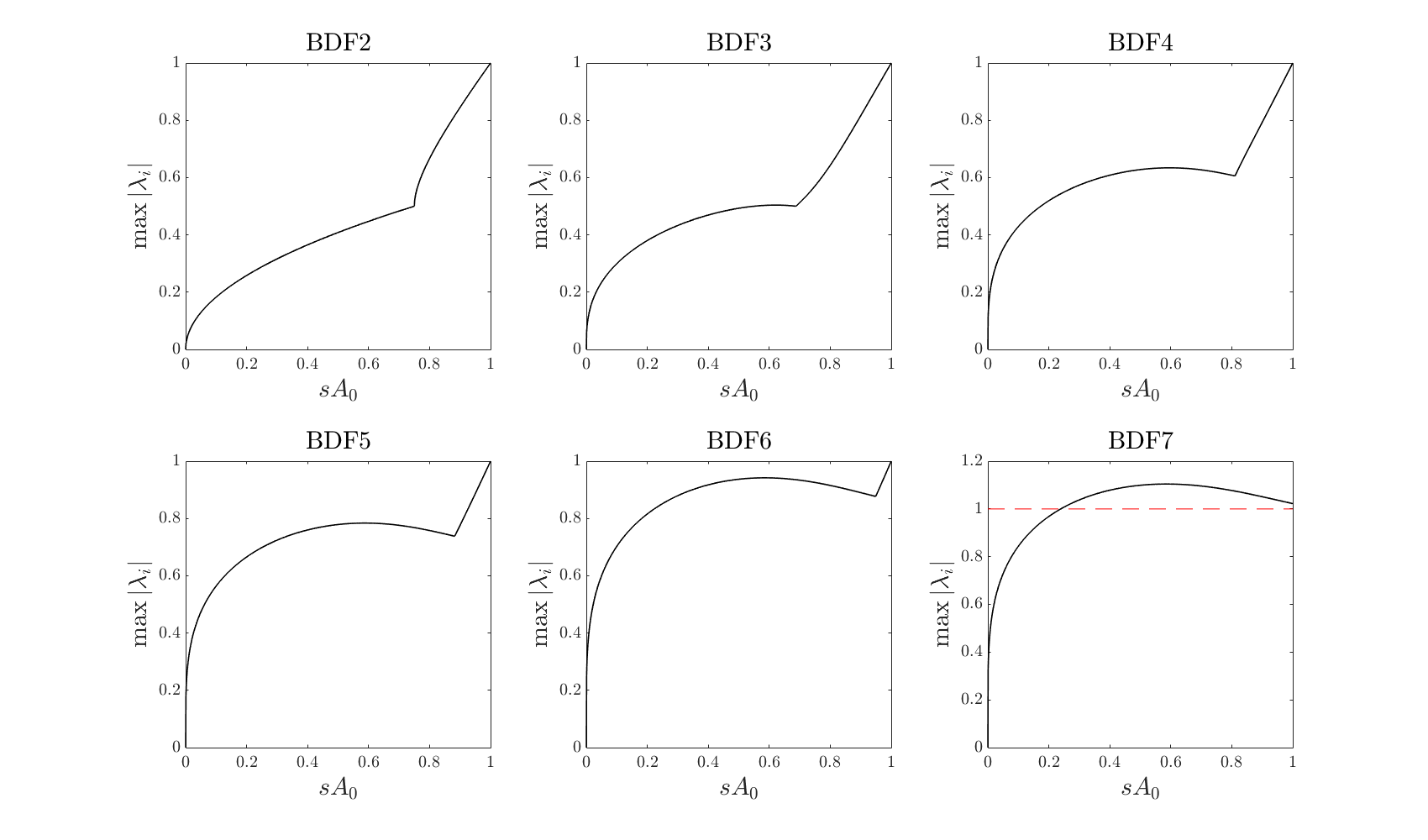
Let 2≤k≤52\leq k\leq 5 and 0<s0<1A0(k)0<s_{0}<\frac{1}{A_{0}^{(k)}}. For 0<s≤s00<s\leq s_{0} the roots λi​(s),i=1,⋯,k\lambda_{i}(s),~i=1,\cdots,k, to the equation in λ\lambda

λk+A1(k)​s​λk−1+⋯+Ak(k)​s=0\lambda^{k}+A_{1}^{(k)}s\lambda^{k-1}+\cdots+A_{k}^{(k)}s=0 (3.15)

satisfy

maxi⁡|λi​(s)|≤λa<1,\max_{i}|\lambda_{i}(s)|\leq\lambda_{a}<1, (3.16)

where λa>0\lambda_{a}>0 depends only on s0.s_{0}.

Remark 3.1.

We first verify this lemma numerically. Figure 2 plots the maxi⁡|λi​(s)|\max_{i}|\lambda_{i}(s)| w.r.t. ss for different BDFkk with 2≤k≤72\leq k\leq 7. It can be seen that this lemma holds true for BDFkk, 2≤k≤62\leq k\leq 6, but not for BDF7. In fact, it is well-known that BDFkk is unstable when k≥7k\geq 7.

Refer to caption
Figure 2. maxi⁡|λi​(s)|\max_{i}|\lambda_{i}(s)| w.r.t. ss for different BDFkk, 2≤k≤72\leq k\leq 7.
Proof.

In the BDF22 case, the proof is trivial and is omitted here. Next, we prove the cases of k=3,4k=3,4 based on the discriminant of algebraic equation, while for the case of k=5k=5, we prove it based on constructing a meromorphic function associated with the polynomial.

BDF33 case. The algebraic equation (3.15) reads as

F3​(λ,s)=λ3−3​s​λ2+32​s​λ−13​s=0,s∈(0,611).F_{3}(\lambda,s)=\lambda^{3}-3s\lambda^{2}+\frac{3}{2}s\lambda-\frac{1}{3}s=0,\quad s\in\left(0,\frac{6}{11}\right). (3.17)

It is known that the discriminant of a cubic polynomial equation a​x3+b​x2+c​x+d=0ax^{3}+bx^{2}+cx+d=0 is

△3=b2​c2−4​a​c3−4​b3​d−27​a2​d2+18​a​b​c​d.\triangle_{3}=b^{2}c^{2}-4ac^{3}-4b^{3}d-27a^{2}d^{2}+18abcd.

If △3<0\triangle_{3}<0, then the cubic polynomial equation admits one real root and one pair of non-real complex conjugate roots. By a simple computation, we obtain the discriminant for (3.17) as

△3=−3​s2+272​s3−634​s4<0fors∈(0,611).\triangle_{3}=-3s^{2}+\frac{27}{2}s^{3}-\frac{63}{4}s^{4}<0\quad\mbox{for}\quad s\in\left(0,\frac{6}{11}\right). (3.18)

Therefore, (3.17) admits only one real root and two complex conjugate roots. Since

∂sF3​(λ,s)=−3​λ2+32​λ−13<0forλ∈ℝ,\partial_{s}F_{3}(\lambda,s)=-3\lambda^{2}+\frac{3}{2}\lambda-\frac{1}{3}<0\quad\mbox{for}\quad\lambda\in\mathbb{R},

we have

F3​(1,s)>F3​(1,611)=0fors∈(0,611).F_{3}(1,s)>F_{3}\left(1,\frac{6}{11}\right)=0\quad\mbox{for}\quad s\in\left(0,\frac{6}{11}\right).

On the other hand,

F3​(12​s,s)=−s⁡(58​s2−34​s+13)<0fors∈(0,611).F_{3}\left(\frac{1}{2}s,s\right)=-s\left(\frac{5}{8}s^{2}-\frac{3}{4}s+\frac{1}{3}\right)<0\quad\mbox{for}\quad s\in\left(0,\frac{6}{11}\right).

Then, the only real root of (3.17) satisfies

λ1​(s)∈(12​s,1)fors∈(0,611).\lambda_{1}(s)\in\left(\frac{1}{2}s,1\right)\quad\mbox{for}\quad s\in\left(0,\frac{6}{11}\right). (3.19)

Since λ1​(s)​λ2​(s)​λ3​(s)=−13​s\lambda_{1}(s)\lambda_{2}(s)\lambda_{3}(s)=-\frac{1}{3}s and λ2​(s)=λ3​(s)¯\lambda_{2}(s)=\overline{\lambda_{3}(s)}, we have

|λ2​(s)|=|λ3​(s)|<23<1fors∈(0,611).|\lambda_{2}(s)|=|\lambda_{3}(s)|<\sqrt{\frac{2}{3}}<1\quad\mbox{for}\quad s\in\left(0,\frac{6}{11}\right). (3.20)

Hence, we proved the conclusion (3.16) for BDF3.3.

BDF44 case. The characteristic equation reads

F4​(λ,s)=λ4−4​s​λ3+3​s​λ2−43​s​λ+14​s=0,s∈(0,1225).F_{4}(\lambda,s)=\lambda^{4}-4s\lambda^{3}+3s\lambda^{2}-\frac{4}{3}s\lambda+\frac{1}{4}s=0,~s\in\left(0,\frac{12}{25}\right). (3.21)

The discriminant for quartic polynomial equation

a​x4+b​x3+c​x2+d​x+e=0ax^{4}+bx^{3}+cx^{2}+dx+e=0

is

△4=\displaystyle\triangle_{4}= 256​a3​e3−192​a2​b​d​e2−128​a2​c2​e2+144​a2​c​d2​e−27​a2​d4\displaystyle 256a^{3}e^{3}-192a^{2}bde^{2}-128a^{2}c^{2}e^{2}+144a^{2}cd^{2}e-27a^{2}d^{4}
+144​a​b2​c​e2−6​a​b2​d2​e−80​a​b​c2​d​e+18​a​b​c​d3+16​a​c4​e−4​a​c3​d2\displaystyle+144ab^{2}ce^{2}-6ab^{2}d^{2}e-80abc^{2}de+18abcd^{3}+16ac^{4}e-4ac^{3}d^{2}
−27​b4​e2+18​b3​c​d​e−4​b3​d3−4​b2​c3​e+b2​c2​d2.\displaystyle-27b^{4}e^{2}+18b^{3}cde-4b^{3}d^{3}-4b^{2}c^{3}e+b^{2}c^{2}d^{2}.

If △4<0\triangle_{4}<0, then quartic polynomial equation has two distinct real roots and two complex conjugate non-real roots. While if △4>0\triangle_{4}>0, P=8​a​c−3​b2>0P=8ac-3b^{2}>0, the quartic equation has two pairs of non-real complex conjugate roots. By tedious computation, we see that the discriminant for (3.21) is

△4=4​s3−883​s4+2203​s5−169627​s6​{>0fors∈(0,38),<0fors∈(38,1225),\triangle_{4}=4s^{3}-\frac{88}{3}s^{4}+\frac{220}{3}s^{5}-\frac{1696}{27}s^{6}\begin{cases}>0\quad\mbox{for}\quad s\in\left(0,\frac{3}{8}\right),\\ \\ <0\quad\mbox{for}\quad s\in\left(\frac{3}{8},\frac{12}{25}\right),\end{cases} (3.22)

and P=24​s−48​s2>0P=24s-48s^{2}>0 for x∈(0,38).x\in\left(0,\frac{3}{8}\right). Hence, equation (3.21) admits two real roots and one pair of complex conjugate roots when s∈(38,1225)s\in\left(\frac{3}{8},\frac{12}{25}\right) and two pairs of complex conjugate roots when s∈(0,38)s\in\left(0,\frac{3}{8}\right). Note that for s=38s=\frac{3}{8}, the equation (3.21) possesses repeated real roots and a pair of complex conjugate roots.

Case 1. s∈[38,1225)s\in\left[\frac{3}{8},\frac{12}{25}\right). When s=1225s=\frac{12}{25}, equation (3.21) admits two real roots 11 and λ∗≈0.3814\lambda_{*}\approx 0.3814. We notice that

∂sF4​(λ,s)=−4​λ3+3​λ2−43​λ+14<0forλ∈(0.32,1).\partial_{s}F_{4}(\lambda,s)=-4\lambda^{3}+3\lambda^{2}-\frac{4}{3}\lambda+\frac{1}{4}<0\quad\mbox{for}\quad\lambda\in\left(0.32,1\right).

It follows that

F4​(1,s)>F4​(1,1225)fors∈(0,1225),F_{4}(1,s)>F_{4}\left(1,\frac{12}{25}\right)\quad\mbox{for}\quad s\in\left(0,\frac{12}{25}\right),

and

F4​(λ∗,s)>F4​(λ∗,1225)fors∈(0,1225).F_{4}(\lambda_{*},s)>F_{4}\left(\lambda_{*},\frac{12}{25}\right)\quad\mbox{for}\quad s\in\left(0,\frac{12}{25}\right).

This implies for any s∈[38,1225)s\in\left[\frac{3}{8},\frac{12}{25}\right), the two real roots λ1​(s),λ2​(s)\lambda_{1}(s),\lambda_{2}(s) are locked in (λ∗,1)(\lambda_{*},1) (see Figure 3 for a schematic diagram). On the other hand the pair of complex conjugate roots satisfy

|λ3​(s)|=|λ4​(s)|<s4⋅1λ∗2≤325⋅10.38132<0.92fors∈[38,1225).|\lambda_{3}(s)|=|\lambda_{4}(s)|<\sqrt{\frac{s}{4}\cdot\frac{1}{\lambda_{*}^{2}}}\leq\sqrt{\frac{3}{25}\cdot\frac{1}{0.3813^{2}}}<0.92\quad\mathrm{for}\quad s\in\left[\frac{3}{8},\frac{12}{25}\right).

Hence, in this case, we proved that maxi⁡|λi|<1.\max_{i}|\lambda_{i}|<1.

Refer to caption
Figure 3. Schematic diagram of F⁡(λ,s)F(\lambda,s) in BDF44 case.

Case 2. s∈(0,38)s\in\left(0,\frac{3}{8}\right). In this case the equation (3.21) admits two pairs of complex conjugate roots. Denoted them by c1,c¯1,c2,c¯2c_{1},\bar{c}_{1},c_{2},\bar{c}_{2}. Clearly,

{ℜ⁡(c1)+ℜ⁡(c2)=2​s,|c1|2+|c2|2+4​ℜ⁡(c1)​ℜ⁡(c2)=3​s,|c1|2​ℜ⁡(c2)+|c2|2​ℜ⁡(c1)=23​s,|c1|2​|c2|2=14​s.\begin{cases}\Re(c_{1})+\Re(c_{2})=2s,\\ |c_{1}|^{2}+|c_{2}|^{2}+4\Re(c_{1})\Re(c_{2})=3s,\\ |c_{1}|^{2}\Re(c_{2})+|c_{2}|^{2}\Re(c_{1})=\frac{2}{3}s,\\ |c_{1}|^{2}|c_{2}|^{2}=\frac{1}{4}s.\end{cases} (3.23)

Without loss of generality, we may assume from the last equation in (3.23) that

|c1|2≥1>14​s≥|c2|2.|c_{1}|^{2}\geq 1>\frac{1}{4}s\geq|c_{2}|^{2}. (3.24)

Together with the first and third equation in (3.23), we get

ℜ⁡(c1)=s⁡(2​|c1|2−23)|c1|2−|c2|2>0,ℜ⁡(c2)=s⁡(−2​|c2|2+23)|c1|2−|c2|2>0.\Re(c_{1})=\frac{s(2|c_{1}|^{2}-\frac{2}{3})}{|c_{1}|^{2}-|c_{2}|^{2}}>0,\quad\Re(c_{2})=\frac{s(-2|c_{2}|^{2}+\frac{2}{3})}{|c_{1}|^{2}-|c_{2}|^{2}}>0. (3.25)

Consequently,

|c1|2−|c2|2=3​s−4​ℜ⁡(c1)​ℜ⁡(c2)−2​|c2|2<3​s.|c_{1}|^{2}-|c_{2}|^{2}=3s-4\Re(c_{1})\Re(c_{2})-2|c_{2}|^{2}<3s. (3.26)

Substituting (3.25) into the second equation in (3.23), we have

3​s\displaystyle 3s =|c1|2+|c2|2+4​s2​(2​|c1|2−23)​(−2​|c2|2+23)(|c1|2−|c2|2)2\displaystyle=|c_{1}|^{2}+|c_{2}|^{2}+\frac{4s^{2}(2|c_{1}|^{2}-\frac{2}{3})(-2|c_{2}|^{2}+\frac{2}{3})}{(|c_{1}|^{2}-|c_{2}|^{2})^{2}} (3.27)
≥by​(3.26)|c1|2+|c2|2+4​s2​(43​(|c1|2+|c2|2)−4​|c1|2​|c2|2−49)(3​s)2\displaystyle\stackrel{{\scriptstyle\text{by}~\eqref{3.27}}}{{\geq}}|c_{1}|^{2}+|c_{2}|^{2}+\frac{4s^{2}(\frac{4}{3}(|c_{1}|^{2}+|c_{2}|^{2})-4|c_{1}|^{2}|c_{2}|^{2}-\frac{4}{9})}{(3s)^{2}}
=by​|c1|2​|c2|2=14​s|c1|2+|c2|2+49​(43​(|c1|2+|c2|2)−s−49)\displaystyle\stackrel{{\scriptstyle\text{by}~|c_{1}|^{2}|c_{2}|^{2}=\frac{1}{4}s}}{{=}}|c_{1}|^{2}+|c_{2}|^{2}+\frac{4}{9}\left(\frac{4}{3}(|c_{1}|^{2}+|c_{2}|^{2})-s-\frac{4}{9}\right)
≥by​|c1|2+|c2|2≥11+1627−1681−49​s=11381−49​s,\displaystyle\stackrel{{\scriptstyle\text{by}~|c_{1}|^{2}+|c_{2}|^{2}\geq 1}}{{\geq}}1+\frac{16}{27}-\frac{16}{81}-\frac{4}{9}s=\frac{113}{81}-\frac{4}{9}s,

which implies that s>113279>38s>\frac{113}{279}>\frac{3}{8}. Thus we arrive at a contradiction. Therefore, we finish the proof for this case.

BDF55 case. The algebraic equation reads

F5​(λ,s)=λ5−5​s​λ4+5​s​λ3−103​s​λ2+54​s​λ−15​s,s∈(0,60137).F_{5}(\lambda,s)=\lambda^{5}-5s\lambda^{4}+5s\lambda^{3}-\frac{10}{3}s\lambda^{2}+\frac{5}{4}s\lambda-\frac{1}{5}s,\quad s\in\left(0,\frac{60}{137}\right). (3.28)

For any s∈(0,60137),s\in\left(0,\frac{60}{137}\right), we consider the following meromorphic function ℱs​(z)\mathcal{F}_{s}(z) defined in complex domain

ℱs​(z)=F5​(z,s)z5−13760​s​z4.\mathcal{F}_{s}(z)=\dfrac{F_{5}(z,s)}{z^{5}-\frac{137}{60}sz^{4}}. (3.29)

It is easy to see that z5−13760​s​z4z^{5}-\frac{137}{60}sz^{4} never vanishes in |z|≥1|z|\geq 1 whenever s∈(0,60137).s\in\left(0,\frac{60}{137}\right). Therefore ℱs​(z)\mathcal{F}_{s}(z) defines a holomorphic function for |z|≥1.|z|\geq 1. It is easy to see that

lim|z|→∞ℱs​(z)=1>0.\lim_{|z|\to\infty}\mathcal{F}_{s}(z)=1>0. (3.30)

Next, we prove that

ℜ⁡(ℱs​(z))>0for|z|≥1​and​s∈(0,60137),\Re(\mathcal{F}_{s}(z))>0\quad\mbox{for}\quad|z|\geq 1~\mbox{and}~s\in\left(0,\frac{60}{137}\right), (3.31)

implying that ℱs​(z)\mathcal{F}_{s}(z) will not vanish in |z|≥1|z|\geq 1.

Note that ℜ⁡(ℱs​(z))\Re(\mathcal{F}_{s}(z)) is harmonic when |z|>1|z|>1. According to the maximum principle of harmonic function and (3.30), to prove (3.31), it is sufficient to show that

ℜ⁡(ℱs​(z))>0for|z|=1​and​s∈(0,60137),\Re(\mathcal{F}_{s}(z))>0\quad\mbox{for}\quad|z|=1~\mbox{and}~s\in\left(0,\frac{60}{137}\right), (3.32)

which is equivalent to

ℜ⁡((1−5​s​z¯+5​s​z¯2−103​s​z¯3+54​s​z¯4−15​s​z¯5)​(1−13760​s​z))>0,\Re\left(\left(1-5s\bar{z}+5s\bar{z}^{2}-\frac{10}{3}s\bar{z}^{3}+\frac{5}{4}s\bar{z}^{4}-\frac{1}{5}s\bar{z}^{5}\right)\left(1-\frac{137}{60}sz\right)\right)>0, (3.33)

for any |z|=1|z|=1 and s∈(0,60137)s\in\left(0,\frac{60}{137}\right), where z¯\bar{z} denotes the conjugate of zz.

We write ℜ⁡(z)\Re(z) as xx and |x|≤1|x|\leq 1, then by the trigonometric identities and tedious computations, we have

ℜ⁡((1−5​s​z¯+5​s​z¯2−103​s​z¯3+54​s​z¯4−15​s​z¯5)​(1−13760​s​z))=1+A⁡(x)​s+B⁡(x)​s2,\displaystyle\Re\left(\left(1-5s\bar{z}+5s\bar{z}^{2}-\frac{10}{3}s\bar{z}^{3}+\frac{5}{4}s\bar{z}^{4}-\frac{1}{5}s\bar{z}^{5}\right)\left(1-\frac{137}{60}sz\right)\right)=1+A(x)s+B(x)s^{2}, (3.34)

where

A⁡(x)=\displaystyle A(x)=~ −154+10360​x−283​x3+10​x4−165​x5,\displaystyle-\frac{15}{4}+\frac{103}{60}x-\frac{28}{3}x^{3}+10x^{4}-\frac{16}{5}x^{5},
B⁡(x)=\displaystyle B(x)=~ 959225−13748​x+2603225​x2−13712​x3+27475​x4.\displaystyle\frac{959}{225}-\frac{137}{48}x+\frac{2603}{225}x^{2}-\frac{137}{12}x^{3}+\frac{274}{75}x^{4}.

Regarding the right-hand side of (3.34) as a quadratic polynomial in ss, we derive the discriminant

A2​(x)−4​B​(x)=\displaystyle A^{2}(x)-4B(x)= −107513600−3524​x−1559833600​x2+3473​x3−27373225​x4+1753​x5\displaystyle-\frac{10751}{3600}-\frac{35}{24}x-\frac{155983}{3600}x^{2}+\frac{347}{3}x^{3}-\frac{27373}{225}x^{4}+\frac{175}{3}x^{5} (3.35)
+17128225​x6−5603​x7+239615​x8−64​x9+25625​x10.\displaystyle+\frac{17128}{225}x^{6}-\frac{560}{3}x^{7}+\frac{2396}{15}x^{8}-64x^{9}+\frac{256}{25}x^{10}.

In Figure 4 given by Matlab, we can see that the polynomial defined on the right-hand side of (3.35) admits two real roots in ℝ\mathbb{R}, they are xs≈−0.908x_{s}\approx-0.908 and 11. The discriminant is negative when xs<x<1x_{s}<x<1. On the other hand, it can be shown that B⁡(x)>0B(x)>0 for −1≤x≤1-1\leq x\leq 1 and A⁡(x)>0A(x)>0 for −1≤x<xs-1\leq x<x_{s}. As a consequence, 1+A⁡(x)​s+B⁡(x)​s2>01+A(x)s+B(x)s^{2}>0 for −1≤x<xs,s∈(0,60137).-1\leq x<x_{s},~s\in\left(0,\frac{60}{137}\right). While if x=1x=1, the quadratic polynomial is

1+A⁡(x)​s+B⁡(x)​s2=(1−13760​s)2>0fors∈(0,60137).1+A(x)s+B(x)s^{2}=\left(1-\frac{137}{60}s\right)^{2}>0\quad\mbox{for}\quad s\in\left(0,\frac{60}{137}\right).

Hence, we have shown that (3.33) holds for all |x|≤1|x|\leq 1 and the claim (3.31) then holds. Therefore, ℱs​(z)\mathcal{F}_{s}(z) never vanishes in |z|≥1|z|\geq 1 for s∈(0,60137).s\in\left(0,\frac{60}{137}\right). It follows that

F5​(s,z)​admits no roots in​|z|≥1fors∈(0,60137).F_{5}(s,z)~\mbox{admits no roots in}~|z|\geq 1\quad\mbox{for}\quad s\in\left(0,\frac{60}{137}\right). (3.36)

It is not difficult to check that all roots of F5​(s,z)=0F_{5}(s,z)=0 are in the unit ball if ss is close to 00. Thus, we proved the conclusion (3.16) for BDF5 case.

Refer to caption
Figure 4. A⁡(x)A(x), B⁡(x)B(x), and A2​(x)−4​B​(x)A^{2}(x)-4B(x) w.r.t. xx for BDF55 case.

∎

Remark 3.2.

It is also possible to work out a proof for BDF44 by following the meromorphic approach in the BDF55 case.

Lemma 3.2.

Let 0<s0<1A0(k)0<s_{0}<\frac{1}{A_{0}^{(k)}}. Consider the matrix

M⁡(s)=(−A1(k)​s−A2(k)​s⋯−Ak−1(k)​s−Ak(k)​s10⋯0001⋯00⋱00⋯10),M(s)=\left(\begin{matrix}-A_{1}^{(k)}s&-A_{2}^{(k)}s&\cdots&-A_{k-1}^{(k)}s&-A_{k}^{(k)}s\\ 1&0&\cdots&0&0\\ 0&1&\cdots&0&0\\ \vdots&\vdots&\ddots&\vdots&\vdots\\ 0&0&\cdots&1&0\end{matrix}\right), (3.37)

where 0<s≤s0.0<s\leq s_{0}. There exists an integer n0≥1n_{0}\geq 1 which depends on s0s_{0} such that

sup0<s≤s0supx∈ℝk,|x|=1|M​(s)n0​x|≤ϵ0<1,\sup_{0<s\leq s_{0}}\sup_{x\in\mathbb{R}^{k},|x|=1}|M(s)^{n_{0}}x|\leq\epsilon_{0}<1, (3.38)

where ϵ0>0\epsilon_{0}>0 depends only on s0s_{0} and |x|=∑i=1k|xi|2|x|=\sqrt{\sum_{i=1}^{k}|x_{i}|^{2}} denotes the usual ℓ2\ell^{2}-norm on ℝk.\mathbb{R}^{k}.

Proof.

First we notice that

M​(s)k=s​Mk​(s),M(s)^{k}=sM_{k}(s), (3.39)

where all entries of Mk​(s)M_{k}(s) are either constants or polynomials of ss. Therefore, if s1s_{1} is sufficiently small, then we have

sup0<s≤s1supx∈ℝk,|x|=1|M​(s)k​x|≤12.\sup_{0<s\leq s_{1}}\sup_{x\in\mathbb{R}^{k},|x|=1}|M(s)^{k}x|\leq\frac{1}{2}. (3.40)

We now focus on the regime s1≤s≤s0<1A0s_{1}\leq s\leq s_{0}<\frac{1}{A_{0}}. Consider a fixed s∗∈[s1,s0]s_{*}\in[s_{1},s_{0}]. By the above lemma, there exists n∗n_{*} depending on s∗s_{*} such that

supx∈ℝk,|x|=1|M​(s∗)n∗​x|≤ϵ∗<1,\sup_{x\in\mathbb{R}^{k},~|x|=1}|M(s_{*})^{n_{*}}x|\leq\epsilon_{*}<1,

where ϵ∗\epsilon_{*} also depends on s∗s_{*}. Perturbing around s∗s_{*} we can find a small neighborhood J∗J_{*} around s∗s_{*} such that

supx∈ℝk,|x|=1|M​(s)n∗​x|≤ϵ1<1,∀s∈J∗,\sup_{x\in\mathbb{R}^{k},~|x|=1}|M(s)^{n_{*}}x|\leq\epsilon_{1}<1,\quad\forall s\in J_{*},

where ϵ1\epsilon_{1} depends only on s∗.s_{*}. By a covering argument, we conclude that there exist n0n_{0} and ϵ0\epsilon_{0} such that (3.38) is satisfied. ∎

Remark 3.3.

The convergence analysis of the BDFkk/EPkk scheme can be done similarly as in the BDF33 case (cf. [13]).

Acknowledgement. The research of W. Yang is supported by NSFC Grants 11801550, 11871470, and 12171456. The work of C. Quan is supported by NSFC Grant 11901281, the Guangdong Basic and Applied Basic Research Foundation (2020A1515010336), and the Stable Support Plan Program of Shenzhen Natural Science Fund (Program Contract No. 20200925160747003).

References

  • [1] Arieh Iserles. A First Course in the Numerical Analysis of Differential Equations. Cambridge University Press 1996.
  • [2] Georgios Akrivis, Minghua Chen, Fan Yu, and Zhi Zhou. The energy technique for the six-step BDF method. arXiv preprint arXiv:2007.08924, 2020.
  • [3] Samuel M Allen and John W Cahn. A microscopic theory for antiphase boundary motion and its application to antiphase domain coarsening. Acta Metallurgica, 27(6):1085–1095, 1979.
  • [4] John W Cahn and John E Hilliard. Free energy of a nonuniform system I: Interfacial free energy. The Journal of Chemical Physics, 28(2):258–267, 1958.
  • [5] Wenbin Chen, Sidafa Conde, Cheng Wang, Xiaoming Wang, and Steven M Wise. A linear energy stable scheme for a thin film model without slope selection. Journal of Scientific Computing, 52(3):546–562, 2012.
  • [6] Shaun Clarke and Dimitri D Vvedensky. Origin of reflection high-energy electron-diffraction intensity oscillations during molecular-beam epitaxy: A computational modeling approach. Physical Review Letters, 58(21):2235, 1987.
  • [7] David J Eyre. Unconditionally gradient stable time marching the Cahn-Hilliard equation. MRS online proceedings library archive, 529, 1998.
  • [8] Yonghong Hao, Qiumei Huang, and Cheng Wang. A third order BDF energy stable linear scheme for the no-slope-selection thin film model. arXiv preprint arXiv:2011.01525, 2020.
  • [9] B. Li, J. Yang, and Z. Zhou: Arbitrarily high-order exponential cut-off methods for preserving maximum principle of parabolic equations. SIAM J. Sci. Comput. 42 (2020), pp. A3957–A3978.
  • [10] Dong Li. Effective maximum principles for spectral methods. Annals of Applied Mathematics, 37: 131–290, 2021.
  • [11] Dong Li, Tao Tang, Stability of the Semi-Implicit Method for the Cahn-Hilliard Equation with Logarithmic Potentials. Ann. Appl. Math., 37 (2021), p. 31-60.
  • [12] D. Li, C. Quan, T. Tang, Stability and convergence analysis for the implicit-explicit method to the Cahn-Hilliard equation. Math. Comp.(to appear)
  • [13] Dong Li, Chaoyu Quan, and Wen Yang. The BDF3/EP3 scheme for MBE with no slope selection is stable. Journal on Scientific Computing, 89:33, 2021.
  • [14] Randall J. LeVeque. Finite difference methods for ordinary and partial differential equations: steady-state and time-dependent problems. Society for Industrial and Applied Mathematics, 2007.
  • [15] Christian Lubich, Dhia Mansour, and Chandrasekhar Venkataraman. Backward difference time discretization of parabolic differential equations on evolving surfaces. IMA Journal of Numerical Analysis, 33(4):1365–1385, 2013.
  • [16] Olavi Nevanlinna and F Odeh. Multiplier techniques for linear multistep methods. Numerical Functional Analysis and Optimization, 3(4):377–423, 1981.
  • [17] Jie Shen, Jie Xu, and Jiang Yang. The scalar auxiliary variable (SAV) approach for gradient flows. Journal of Computational Physics, 353:407–416, 2018.
  • [18] Jie Shen and Xiaofeng Yang. Numerical approximations of Allen–Cahn and Cahn–Hilliard equations. Discrete & Continuous Dynamical Systems-A, 28(4):1669, 2010.
  • [19] Cheng Wang, Xiaoming Wang, and Steven M Wise. Unconditionally stable schemes for equations of thin film epitaxy. Discrete & Continuous Dynamical Systems-A, 28(1):405, 2010.
  • [20] Chuanju Xu and Tao Tang. Stability analysis of large time-stepping methods for epitaxial growth models. SIAM Journal on Numerical Analysis, 44(4):1759–1779, 2006.
  • [21] W.W. Mullins. Theory of thermal grooving. Journal of Applied Physics. 28(3), (1957), 333-339.
  • [22] C. Herring. Surface tension as a motivation for sintering In: Kingston, W.E. (Ed.) The Physics of powder Metallurgy, McGraw-Hill, New York.