跳到论文正文
W Papers独立论文阅读器 arXiv:2111.05156 论文正文 计算阅读时间 · 0%
引用这篇论文根据当前论文元数据生成,正式投稿前建议核对。


License: arXiv.org perpetual non-exclusive license
arXiv:2111.05156v2 [math.NA] 04 Aug 2022

Error estimates for Euler discretization of high-index saddle dynamics

Lei Zhang Thanks: Beijing International Center for Mathematical Research, Center for Quantitative Biology, Peking University, Beijing 100871, China (zhangl@math.pku.edu.cn)    Pingwen Zhang Thanks: School of Mathematical Sciences, Laboratory of Mathematics and Applied Mathematics, Peking University, Beijing 100871, China (pzhang@pku.edu.cn).    Xiangcheng Zheng Thanks: School of Mathematical Sciences, Peking University, Beijing 100871, China (zhengxch@outlook.com)
Abstract

High-index saddle dynamics provides an effective means to compute the any-index saddle points and construct the solution landscape. In this paper we prove error estimates for Euler discretization of high-index saddle dynamics with respect to the time step size, which remains untreated in the literature. We overcome the main difficulties that lie in the strong nonlinearity of the saddle dynamics and the orthonormalization procedure in the numerical scheme that is uncommon in standard discretization of differential equations. The derived methods are further extended to study the generalized high-index saddle dynamics for non-gradient systems and provide theoretical support for the accuracy of numerical implementations.

keywords
saddle point, saddle dynamics, solution landscape, Euler scheme, error estimate
AMS
37M05, 37N30, 65L20

1 Introduction

Finding stationary points of nonlinear multivariable energy functions E⁡(x)E({x}) has attracted extensive interest in different scientific communities during the past decades. It plays a crucial role in determining many physical or chemical properties of complex systems, examples of which include the critical nuclei in phase transition [5, 34, 35, 36], defects in liquid crystals [11, 24], self-assembly of polymers [12, 25], molecular clusters [1, 3], and artificial neural network [9]. According to Morse theory [21], the local stability of stationary points, including both stable minima and unstable saddle points, can be characterized by the Morse index. The (Morse) index of a nondegenerate saddle point is the maximal dimension of a subspace on which its Hessian matrix is negative definite, i.e. the number of negative eigenvalues of the Hessian matrix. In particular, the stable stationary point (minimizer) can be regarded as an index-0 saddle point with no unstable direction.

Due to the complex geometric structures of the energy functions and the unstable nature of saddle points, how to efficiently compute multiple stationary points remains a challenging problem [3, 7, 18, 20]. Most existing efforts focus on finding the index-1 saddle point or transition state, i.e. a stationary point where the Hessian has one and only one negative eigenvalue. One of the popular approaches is the class of surface walking methods [34]. In particular, the dimer-type method [15, 33, 37] and the gentlest ascent dynamics [6], as the representatives of the surface walking methods, were developed to compute the index-1 saddle points. Recently, inspired by the optimization-based shrinking dimer method [37], the high-index saddle dynamics (HiSD) was proposed to search for any-index saddle points [31]. The HiSD method provides an efficient tool to construct the solution landscape of the energy systems, which describes a pathway map that starts with a parent state (the highest-index saddle point) and then relates the low-index saddle points down to all the minimizers [29]. The solution landscape approach has been applied to study various physical systems such as liquid crystals [13, 14, 32], polymers [26], and quasicrystals [28]. Moreover, based on the HiSD method, a generalized high-index saddle dynamics (GHiSD) was further proposed to compute the any-index saddle points and solution landscapes of dynamical (non-gradient) systems [30].

Despite the sustained development of the saddle-point searching algorithms, the rigorous numerical analysis on them are still far from well-developed. Some existing studies mainly focus on the index-1 saddle points. For instance, in [33], the time discretization of the shrinking dimer dynamics was studied, and the linear local asymptotic stability analysis and optimal error reduction rates were carried out. Global convergence and nonlinear asymptotic stability were also illustrated for some specific systems. In [10], the dimer method with linesearch for the step size and the preconditioning was investigated. Local convergence and error reduction were proved and, in particular, the O⁡(l2)O(l^{2}) accuracy between the stationary point of the algorithm and the saddle was proved where ll refers to the dimer length. In [16], the existing local convergence results for dimer-type and gentlest ascent dynamics methods were extended by developing an improved estimate on the region of attraction of index-1 saddle points that goes beyond the linearized regime. In [8], a quadratic local convergence rate in terms of number of iterations was proved for an iterative minimization scheme for searching index-1 saddle points of energy functions.

The aforementioned works, which provide asymptotic convergence results of, e.g. xn−x∗x_{n}-x_{*}, where xnx_{n} and x∗x_{*} refer to the numerical solution at the nn-th iteration and the limit (target saddle point) of the scheme, respectively, made significant progress on the theoretical foundation of numerical analysis of the saddle-point searching algorithms. In contrast, the error estimate of xn−x⁡(tn)x_{n}-x(t_{n}), where x⁡(tn)x(t_{n}) represents the exact solution of HiSD at the step tnt_{n}, gives the dynamical pathway convergence of numerical solutions to the saddle dynamics, which provides important physical information, such as the transition pathway [28], and theoretically ensure the accuracy of the constructed solution landscape [29]. Inaccurate computations of the dynamical pathway could lead to missing saddle points and an incomplete solution landscape. Therefore, it is necessary and meaningful to perform the error estimates of xn−x⁡(tn)x_{n}-x(t_{n}) for HiSD, which motivates the investigations in the work. Furthermore, the existing numerical analysis only focuses on the schemes of finding index-1 saddle points, while the corresponding results for numerical methods of finding high-index saddle points in [30, 31] are still unavailable.

Motivated by these discussions, in this paper we aim to prove error estimates for the Euler discretization of HiSD method with respect to the time step size, which focuses more on the dynamics (i.e. the searching pathways between saddle points) than its limit. We emphasize that there exist some essential differences and challenges from the standard methods of ODEs. First, the rigorous numerical analysis on saddle-point searching algorithms is more challenging than gradient descent methods for finding the minima, which remains untreated for the high-index saddle points in particular. For instance, in (27) the left-hand side of the scheme of the ii-th eigenvector viv_{i} is not its numerical approximation vi,nv_{i,n} at the step tnt_{n}, but an intermediate quantity v~i,n\tilde{v}_{i,n}. This is due to the fact that the outcomes {v~i,n}\{\tilde{v}_{i,n}\} of the schemes of {vi}\{v_{i}\} may not be orthonormal and thus need to be further processed in the third equation of (27). Consequently, in order to generate the error equations by subtracting the schemes from the reference equations, we will encounter vi​(tn)−v~i,nv_{i}(t_{n})-\tilde{v}_{i,n} instead of vi​(tn)−vi,nv_{i}(t_{n})-v_{i,n} as in the case of ODE discretizations. A natural idea is to split vi​(tn)−v~i,nv_{i}(t_{n})-\tilde{v}_{i,n} as (vi​(tn)−vi,n)+(vi,n−v~i,n)(v_{i}(t_{n})-v_{i,n})+(v_{i,n}-\tilde{v}_{i,n}), which requires an additional estimate of vi,n−v~i,nv_{i,n}-\tilde{v}_{i,n} that is not common in numerical methods of ODEs. Since {vi,n}\{v_{i,n}\} is generated from {v~i,n}\{\tilde{v}_{i,n}\} via the orthonormalization, careful estimates are required for this procedure, which is intricate and not available in the literature. Furthermore, to support this analysis, novel techniques are developed to overcome the strong nonlinearity of the HiSD to prove several properties of the numerical solutions based on their schemes, which serves as another highlight. The aforementioned issues are the main contributions of the current work and distinguish the proposed methods from the standard numerical analysis of ODEs. By subtle treatments and estimates, we rigorously prove the first-order accuracy of the numerical scheme, which contributes to the numerical theory of HiSD and provides theoretical support for the accuracy of numerical computations.

The rest of the paper is organized as follows: In Section 2 we present formulations of HiSD. In Section 3 we prove the error estimates for Euler discretization of index-1 saddle dynamics. In Section 4 we extend the developed techniques to prove error estimates for the Euler discretization of index-kk saddle dynamics. Numerical experiments are performed in Section 5 to substantiate the theoretical findings. In Section 6 we extend the proposed techniques to study the GHiSD of non-gradient systems, and we finally address the concluding remarks in Section 7.

2 Formulation of high-index saddle dynamics

Given a twice Fréchet differentiable energy functional E⁡(x)E(x) with x∈ℝNx\in\mathbb{R}^{N} and define the corresponding natural force F:ℝN→ℝNF:\mathbb{R}^{N}\rightarrow\mathbb{R}^{N} and the negative Hessian J∈ℝN×NJ\in\mathbb{R}^{N\times N} by F​(x)=−∇E​(x)F(x)=-\nabla E(x) and J⁡(x)=−∇2E​(x)J(x)=-\nabla^{2}E(x). It is clear that J⁡(x)=J​(x)⊤J(x)=J(x)^{\top}. Then the saddle dynamics for an index-kk saddle point (kk-SD) of E⁡(x)E(x) with 1≤k∈ℕ1\leq k\in\mathbb{N} reads [31]

{d​xd​t=β⁡(I−2​∑j=1kvj​vj⊤)​F​(x),d​vid​t=γ⁡(I−vi​vi⊤−2​∑j=1i−1vj​vj⊤)​J​(x)​vi,1≤i≤k\left\{\begin{array}[]{l}\displaystyle\frac{dx}{dt}=\beta\bigg(I-2\sum_{j=1}^{k}v_{j}v_{j}^{\top}\bigg)F(x),\\[5.42003pt] \displaystyle\frac{dv_{i}}{dt}=\gamma\bigg(I-v_{i}v_{i}^{\top}-2\sum_{j=1}^{i-1}v_{j}v_{j}^{\top}\bigg)J(x)v_{i},~~1\leq i\leq k\end{array}\right. (1)

where xx represents a position variable, vi​(i=1,…​k)v_{i}(i=1,...k) are kk directional variables, and β\beta, γ>0\gamma>0 are relaxation parameters. The system (1) was formulated by the minimax optimization framework, and it was shown in [31, Theorem 1] that, under suitable assumptions, a linearly stable solution of (1) is an index-kk saddle point of E⁡(x)E(x) associated with kk eigenvectors corresponding to the kk negative eigenvalues of its Hessian. Furthermore, it is shown in [31] that if the initial values of {vi​(t)}i=1k\{v_{i}(t)\}_{i=1}^{k} for (1) are orthonormal vectors, then

‖vi​(t)‖=1,1≤i≤k,∀t>0.\|v_{i}(t)\|=1,~~1\leq i\leq k,~~\forall t>0. (2)

In particular, the index-1 saddle points attract many interests as they connect different minimizers. This corresponds to the simplest case of (1) with k=1k=1, i.e., 11-SD, which is also equivalent to the gentlest ascent dynamics proposed in [6]

{d​xd​t=β⁡(I−2​v​v⊤)​F​(x),d​vd​t=γ⁡(I−v​v⊤)​J​(x)​v.\left\{\begin{array}[]{l}\displaystyle\frac{dx}{dt}=\beta\big(I-2vv^{\top}\big)F(x),\\[7.22743pt] \displaystyle\frac{dv}{dt}=\gamma\big(I-vv^{\top}\big)J(x)v.\end{array}\right. (3)

Throughout the paper we make the following regular assumptions on the force and the Hessian:

Assumption A: There exists a constant L>0L>0 such that the following linearly growth and Lipschitz conditions hold under the standard l2l^{2} norm ∥⋅∥\|\cdot\| of a vector or a matrix

‖J⁡(x2)−J⁡(x1)‖+|F⁡(x2)−F⁡(x1)|≤L​‖x2−x1‖,‖F⁡(x)‖≤L⁡(1+‖x‖),x,x1,x2∈ℝN.\begin{array}[]{c}\displaystyle\|J(x_{2})-J(x_{1})\|+\|F(x_{2})-F(x_{1})\|\leq L\|x_{2}-x_{1}\|,\\[7.22743pt] \displaystyle\|F(x)\|\leq L(1+\|x\|),~~x,x_{1},x_{2}\in\mathbb{R}^{N}.\end{array}
Remark 2.1.

In many applications, there exist various energy functions EE satisfying the Assumption A, such as the Minyaev-Quapp surface [22]

E⁡(x1,x2)=cos⁡(2​x1)+cos⁡(2​x2)+0.57​cos⁡(2​x1−2​x2)E(x_{1},x_{2})=\cos(2x_{1})+\cos(2x_{2})+0.57\cos(2x_{1}-2x_{2}) (4)

and the Eckhardt surface [4]

E⁡(x1,x2)=exp​(−x12−(x2+1)2)+exp​(−x12−(x2−1)2)+4​exp​(−3​x12+x222)+x222.\begin{array}[]{l}\displaystyle E(x_{1},x_{2})=\text{exp}(-x_{1}^{2}-(x_{2}+1)^{2})\\ \displaystyle\qquad\qquad\qquad+\text{exp}(-x_{1}^{2}-(x_{2}-1)^{2})+4\text{exp}\bigg(-3\frac{x_{1}^{2}+x_{2}^{2}}{2}\bigg)+\frac{x_{2}^{2}}{2}.\end{array} (5)

We then cite the continuous and discrete Gronwall inequalities that will be frequently used in this paper [2].

Lemma 1.

Assume zz, gg and kk are continuous functions on [0,T][0,T], z≥0z\geq 0, k≥0k\geq 0, gg is non-decreasing, and

z⁡(t)≤g⁡(t)+∫0tk⁡(s)​z​(s)​𝑑s,t∈[0,T].z(t)\leq g(t)+\int_{0}^{t}k(s)z(s)ds,~~t\in[0,T].

Then the following estimate holds

z⁡(t)≤g⁡(t)​exp​(∫0tk⁡(s)​𝑑s),t∈[0,T].z(t)\leq g(t)\text{exp}\bigg(\int_{0}^{t}k(s)ds\bigg),~~t\in[0,T].

Assume that the non-negative sequences {zn}n≥1\{z_{n}\}_{n\geq 1} and {kn}n≥1\{k_{n}\}_{n\geq 1} satisfy

zn≤ρ+∑j=1n−1kj​zj,n≥1z_{n}\leq\rho+\sum_{j=1}^{n-1}k_{j}z_{j},~~n\geq 1

for some ρ≥0\rho\geq 0. Then the following estimate holds

zn≤ρ​exp​(∑j=1n−1kj),n≥1.z_{n}\leq\rho\text{exp}\bigg(\sum_{j=1}^{n-1}k_{j}\bigg),~~n\geq 1.

By (2), we multiply the first equation in (1) by x⊤x^{\top} to obtain

12​dd​t​‖x‖2=x⊤​d​xd​t=β​x⊤​F​(x)−2​β​∑j=1kvj⊤​F​(x)​x⊤​vj≤β​‖x‖​‖F⁡(x)​‖+2​β​k‖​x‖​‖F⁡(x)‖≤(1+2​k)​β​L​‖x‖​(1+‖x‖)≤3​(1+2​k)​β​L2​‖x‖2+(1+2​k)​β​L2,\begin{array}[]{rl}\displaystyle\frac{1}{2}\frac{d}{dt}\|x\|^{2}&\displaystyle=x^{\top}\frac{dx}{dt}=\beta x^{\top}F(x)-2\beta\sum_{j=1}^{k}v_{j}^{\top}F(x)x^{\top}v_{j}\\[7.22743pt] &\displaystyle\leq\beta\|x\|\|F(x)\|+2\beta k\|x\|\|F(x)\|\\[7.22743pt] &\displaystyle\leq(1+2k)\beta L\|x\|(1+\|x\|)\\[7.22743pt] &\displaystyle\leq\frac{3(1+2k)\beta L}{2}\|x\|^{2}+\frac{(1+2k)\beta L}{2},\end{array} (6)

which leads to

‖x⁡(t)‖2≤‖x⁡(0)‖2+3​(1+2​k)​β​L​∫0t‖x⁡(s)‖2​𝑑s+(1+2​k)​β​L​t.\displaystyle\|x(t)\|^{2}\leq\|x(0)\|^{2}+3(1+2k)\beta L\int_{0}^{t}\|x(s)\|^{2}ds+(1+2k)\beta Lt. (7)

Then for a terminal time T>0T>0, an application of the Gronwall inequality in Lemma 1 yields

‖x‖2≤(‖x⁡(0)‖2+(1+2​k)​β​L​T)​e3​(1+2​k)​β​L​T=:QT.\|x\|^{2}\leq\big(\|x(0)\|^{2}+(1+2k)\beta LT\big)e^{3(1+2k)\beta LT}=:Q_{T}. (8)

That is, within any terminal time TT, ‖x‖\|x\| can be bounded by some fixed constant QT\sqrt{Q_{T}}, and we thus assume

JT:=max‖x‖≤QT⁡‖J⁡(x)‖.J_{T}:=\max_{\|x\|\leq\sqrt{Q_{T}}}\|J(x)\|.

3 Numerical analysis for index-1 saddle dynamics

In this section, we consider the explicit Euler scheme of 1-SD (3) on the time interval [0,T][0,T] for some T>0T>0 equipped with the initial conditions

x⁡(0)=x0,v⁡(0)=v0,‖v0‖2=1.\displaystyle x(0)=x_{0},~~v(0)=v_{0},~~\|v_{0}\|_{2}=1. (9)

Although this is mathematically a special case of kk-SD (1), it is indeed the most considered case and could elucidate some key ideas of the analysis in a clear manner.

3.1 Explicit Euler scheme

For NT∈ℕN_{T}\in\mathbb{N}, we define a uniform temporal partition of [0,T][0,T] by tn=n​τt_{n}=n\tau for 0≤n≤NT0\leq n\leq N_{T} where τ=T/NT\tau=T/N_{T} stands for the time step size. We then approximate the first-order derivative by the backward Euler scheme at tnt_{n} as follows

d​g​(tn)d​t=g⁡(tn)−g⁡(tn−1)τ+Rng\frac{dg(t_{n})}{dt}=\frac{g(t_{n})-g(t_{n-1})}{\tau}+R_{n}^{g}

where gg refers to xx or vv, and the truncation error ‖Rng‖=O⁡(τ)\|R_{n}^{g}\|=O(\tau). Plugging this discretization into (3) yields

{x⁡(tn)=x⁡(tn−1)+τ​β​(I−2​v​(tn−1)​v​(tn−1)⊤)​F​(x⁡(tn−1))+τ​Rnx,v⁡(tn)=v⁡(tn−1)+τ​γ​(I−v⁡(tn−1)​v​(tn−1)⊤)​J​(x⁡(tn−1))​v​(tn−1)+τ​Rnv.\left\{\begin{array}[]{l}\displaystyle x(t_{n})=x(t_{n-1})+\tau\beta\big(I-2v(t_{n-1})v(t_{n-1})^{\top}\big)F(x(t_{n-1}))+\tau R_{n}^{x},\\[5.42003pt] \displaystyle v(t_{n})=v(t_{n-1})+\tau\gamma\big(I-v(t_{n-1})v(t_{n-1})^{\top}\big)J(x(t_{n-1}))v(t_{n-1})+\tau R_{n}^{v}.\end{array}\right. (10)

Then we drop the truncation errors to obtain the explicit Euler scheme of (3) with the approximations {xn,vn}n=1NT\{x_{n},v_{n}\}_{n=1}^{N_{T}} to {x⁡(tn),v⁡(tn)}n=1NT\{x(t_{n}),v(t_{n})\}_{n=1}^{N_{T}}

{xn=xn−1+τ​β​(I−2​vn−1​vn−1⊤)​F​(xn−1),v~n=vn−1+τ​γ​(I−vn−1​vn−1⊤)​J​(xn−1)​vn−1,vn=v~n‖v~n‖\left\{\begin{array}[]{l}\displaystyle x_{n}=x_{n-1}+\tau\beta\big(I-2v_{n-1}v_{n-1}^{\top}\big)F(x_{n-1}),\\[5.42003pt] \displaystyle\tilde{v}_{n}=v_{n-1}+\tau\gamma\big(I-v_{n-1}v_{n-1}^{\top}\big)J(x_{n-1})v_{n-1},\\[5.42003pt] \displaystyle v_{n}=\frac{\tilde{v}_{n}}{\|\tilde{v}_{n}\|}\end{array}\right. (11)

for 1≤n≤NT1\leq n\leq N_{T}, equipped with the initial conditions (9).

From (11) we find that although v~n\tilde{v}_{n} may not have the unit l2l_{2} norm due to the discretization errors, the normalization procedure in the third equation of (11) ensures ‖vn‖=1\|v_{n}\|=1 in order to preserve the unit length of vv as in the continuous problem (3). We thus multiply xn⊤x_{n}^{\top} on both sides of the first equation of (11) to obtain

‖xn‖2≤‖xn‖​‖xn−1​‖+τ​β‖​xn‖​‖F⁡(xn−1)​‖+τ​β‖​xn‖​‖F⁡(xn−1)‖,\|x_{n}\|^{2}\leq\|x_{n}\|\|x_{n-1}\|+\tau\beta\|x_{n}\|\|F(x_{n-1})\|+\tau\beta\|x_{n}\|\|F(x_{n-1})\|,

which leads to

‖xn‖−‖xn−1‖≤τ​β|F⁡(xn−1)​‖+2​τ​β‖​F​(xn−1)|≤3​τ​β​L​(1+‖xn−1‖).\|x_{n}\|-\|x_{n-1}\|\displaystyle\leq\tau\beta\|F(x_{n-1})\|+2\tau\beta\|F(x_{n-1})\|\leq 3\tau\beta L(1+\|x_{n-1}\|).

Summing up this equation from n=1n=1 to n∗≤NTn^{*}\leq N_{T} yields

‖xn∗‖−‖x0‖≤3​β​L​T+3​τ​β​L​∑n=1n∗‖xn−1‖.\|x_{n^{*}}\|-\|x_{0}\|\leq 3\beta LT+3\tau\beta L\sum_{n=1}^{n^{*}}\|x_{n-1}\|.

Then we apply the discrete Gronwall inequality to conclude that there exists a constant Q¯T\bar{Q}_{T} like (8) such that ‖xn‖≤Q¯T\|x_{n}\|\leq\sqrt{\bar{Q}_{T}} for 0≤n≤NT,0\leq n\leq N_{T}, and we thus assume

J¯T:=max‖x‖≤Q¯T⁡‖J⁡(x)‖.\bar{J}_{T}:=\max_{\|x\|\leq\sqrt{\bar{Q}_{T}}}\|J(x)\|. (12)

3.2 Auxiliary estimate of v~n−vn\tilde{v}_{n}-v_{n}

If we intend to find the error equation of env:=v⁡(tn)−vne^{v}_{n}:=v(t_{n})-v_{n} by subtracting the second equation of (10) from that of (11), the right-hand side of the resulting equation has en−1ve^{v}_{n-1} while the left-hand side is v⁡(tn)−v~nv(t_{n})-\tilde{v}_{n} instead of enve^{v}_{n} due to the normalization, which is uncommon in the context of discretizing differential equations that naturally yields the errors of different time steps on both sides of the error equations. A potential idea to circumvent this issue is to split v⁡(tn)−v~nv(t_{n})-\tilde{v}_{n} as (v⁡(tn)−vn)+(vn−v~n)=env+(vn−v~n)(v(t_{n})-v_{n})+(v_{n}-\tilde{v}_{n})=e^{v}_{n}+(v_{n}-\tilde{v}_{n}), which introduces an additional error vn−v~nv_{n}-\tilde{v}_{n}. In particular, we need to show that the difference vn−v~nv_{n}-\tilde{v}_{n} has the magnitude of O⁡(τ2)O(\tau^{2}) in order to preserve the O⁡(τ)O(\tau) accuracy of the numerical scheme (11), which motivates the following estimate.

Lemma 2.

Under the Assumption A, the following estimate holds

|‖v~n‖−1|≤|‖v~n‖2−1|≤τ2​γ2​J¯T2,1≤n≤NT.\big|\|\tilde{v}_{n}\|-1\big|\leq\big|\|\tilde{v}_{n}\|^{2}-1\big|\leq\tau^{2}\gamma^{2}\bar{J}^{2}_{T},~~1\leq n\leq N_{T}.
Proof.

By ‖vn−1‖=1\|v_{n-1}\|=1 we multiply vn−1⊤v^{\top}_{n-1} on both sides of the second equation of (11) to obtain

vn−1⊤​v~n=vn−1⊤​vn−1+τ​γ​(vn−1⊤​J​(xn−1)​vn−1−vn−1⊤​vn−1​vn−1⊤​J​(xn−1)​vn−1)=1.\begin{array}[]{l}\displaystyle v^{\top}_{n-1}\tilde{v}_{n}=v^{\top}_{n-1}v_{n-1}\\[5.42003pt] \qquad+\tau\gamma\big(v^{\top}_{n-1}J(x_{n-1})v_{n-1}-v^{\top}_{n-1}v_{n-1}v^{\top}_{n-1}J(x_{n-1})v_{n-1}\big)=1.\end{array} (13)

We then multiply v~n⊤\tilde{v}_{n}^{\top} on both sides of the second equation of (11) and apply (13) to obtain

‖v~n‖2=v~n⊤​v~n=v~n⊤​vn−1+τ​γ​(v~n⊤​J​(xn−1)​vn−1−v~n⊤​vn−1​vn−1⊤​J​(xn−1)​vn−1)=1+τ​γ​(v~n⊤​J​(xn−1)​vn−1−vn−1⊤​J​(xn−1)​vn−1)=1+τ​γ​(v~n−vn−1)⊤​J​(xn−1)​vn−1.\begin{array}[]{rl}\|\tilde{v}_{n}\|^{2}&\displaystyle=\tilde{v}_{n}^{\top}\tilde{v}_{n}\\[5.42003pt] &\displaystyle=\tilde{v}_{n}^{\top}v_{n-1}+\tau\gamma\big(\tilde{v}_{n}^{\top}J(x_{n-1})v_{n-1}-\tilde{v}_{n}^{\top}v_{n-1}v_{n-1}^{\top}J(x_{n-1})v_{n-1}\big)\\[5.42003pt] &\displaystyle=1+\tau\gamma\big(\tilde{v}_{n}^{\top}J(x_{n-1})v_{n-1}-v_{n-1}^{\top}J(x_{n-1})v_{n-1}\big)\\[5.42003pt] &\displaystyle=1+\tau\gamma\big(\tilde{v}_{n}-v_{n-1}\big)^{\top}J(x_{n-1})v_{n-1}.\end{array} (14)

Subtracting (13) from (14) we get

(v~n−vn−1)⊤​v~n=τ​γ​(v~n−vn−1)⊤​J​(xn−1)​vn−1.\big(\tilde{v}_{n}-v_{n-1}\big)^{\top}\tilde{v}_{n}=\tau\gamma\big(\tilde{v}_{n}-v_{n-1}\big)^{\top}J(x_{n-1})v_{n-1}. (15)

By ‖vn−1‖=1\|v_{n-1}\|=1 and (13) we have

(v~n−vn−1)⊤​vn−1=v~n⊤​vn−1−vn−1⊤​vn−1=1−1=0,\big(\tilde{v}_{n}-v_{n-1}\big)^{\top}v_{n-1}=\tilde{v}_{n}^{\top}v_{n-1}-v_{n-1}^{\top}v_{n-1}=1-1=0,

and we apply this equality and (15) to obtain

‖v~n−vn−1‖2=(v~n−vn−1)⊤​(v~n−vn−1)=(v~n−vn−1)⊤​v~n=τ​γ​(v~n−vn−1)⊤​J​(xn−1)​vn−1≤τ​γ​‖v~n−vn−1‖​‖J⁡(xn−1)‖​‖vn−1‖≤τ​γ​J¯T​‖v~n−vn−1‖,\begin{array}[]{rl}\displaystyle\|\tilde{v}_{n}-v_{n-1}\|^{2}&\displaystyle=(\tilde{v}_{n}-v_{n-1})^{\top}(\tilde{v}_{n}-v_{n-1})\\[5.42003pt] &\displaystyle=(\tilde{v}_{n}-v_{n-1})^{\top}\tilde{v}_{n}=\tau\gamma\big(\tilde{v}_{n}-v_{n-1}\big)^{\top}J(x_{n-1})v_{n-1}\\[5.42003pt] &\displaystyle\leq\tau\gamma\|\tilde{v}_{n}-v_{n-1}\|\|J(x_{n-1})\|\|v_{n-1}\|\\[5.42003pt] &\displaystyle\leq\tau\gamma\bar{J}_{T}\|\tilde{v}_{n}-v_{n-1}\|,\end{array}

that is,

‖v~n−vn−1‖≤τ​γ​J¯T.\displaystyle\|\tilde{v}_{n}-v_{n-1}\|\leq\tau\gamma\bar{J}_{T}. (16)

Note that (14) implies

‖v~n‖2−1=τ​γ​(v~n−vn−1)⊤​J​(xn−1)​vn−1.\displaystyle\|\tilde{v}_{n}\|^{2}-1=\tau\gamma\big(\tilde{v}_{n}-v_{n-1}\big)^{\top}J(x_{n-1})v_{n-1}. (17)

We invoke (16) in (17) to obtain

|‖v~n‖2−1|≤τ​γ​‖v~n−vn−1‖​‖J⁡(xn−1)‖|vn−1|≤τ2​γ2​J¯T2.\displaystyle\big|\|\tilde{v}_{n}\|^{2}-1\big|\leq\tau\gamma\|\tilde{v}_{n}-v_{n-1}\|\|J(x_{n-1})\|\|v_{n-1}\|\leq\tau^{2}\gamma^{2}\bar{J}^{2}_{T}. (18)

We incorporate this estimate with

|‖v~n‖2−1|=(‖v~n‖+1)​|‖v~n‖−1|≥|‖v~n‖−1|\displaystyle\big|\|\tilde{v}_{n}\|^{2}-1\big|=\big(\|\tilde{v}_{n}\|+1\big)\big|\|\tilde{v}_{n}\|-1\big|\geq\big|\|\tilde{v}_{n}\|-1\big| (19)

to complete the proof. ∎

Corollary 3.

Under the Assumption A, the following estimate holds

‖v~n−vn‖≤τ2​γ2​J¯T2,1≤n≤NT.\|\tilde{v}_{n}-v_{n}\|\leq\tau^{2}\gamma^{2}\bar{J}^{2}_{T},~~1\leq n\leq N_{T}.
Proof.

We subtract v~n\tilde{v}_{n} from vnv_{n} to find

v~n−vn=v~n−v~n‖v~n‖=v~n‖v~n‖​(‖v~n‖−1).\tilde{v}_{n}-v_{n}=\tilde{v}_{n}-\frac{\tilde{v}_{n}}{\|\tilde{v}_{n}\|}=\frac{\tilde{v}_{n}}{\|\tilde{v}_{n}\|}\big(\|\tilde{v}_{n}\|-1\big).

Thus we apply Lemma 2 to immediately obtain

‖v~n−vn‖=‖v~n‖‖v~n‖​|‖v~n‖−1|≤τ2​γ2​J¯T2,\|\tilde{v}_{n}-v_{n}\|=\frac{\|\tilde{v}_{n}\|}{\|\tilde{v}_{n}\|}\big|\|\tilde{v}_{n}\|-1\big|\leq\tau^{2}\gamma^{2}\bar{J}^{2}_{T},

which completes the proof. ∎

3.3 Error estimates

Define the errors by

enx:=x⁡(tn)−xn,env:=v⁡(tn)−vn,1≤n≤NT.e^{x}_{n}:=x(t_{n})-x_{n},~~e^{v}_{n}:=v(t_{n})-v_{n},~~1\leq n\leq N_{T}.

We first bound enxe^{x}_{n} in terms of enve^{v}_{n} in the following theorem.

Theorem 4.

Suppose the Assumption A holds. Then the following estimate holds

‖enx‖≤Q​τ​∑m=1n−1‖emv‖+Q​τ,1≤n≤NT.\|e^{x}_{n}\|\leq Q\tau\sum_{m=1}^{n-1}\|e^{v}_{m}\|+Q\tau,~~1\leq n\leq N_{T}.

Here QQ depends on LL, TT and β\beta but is independent from τ\tau, nn and NTN_{T}.

Proof.

We subtract the first equation of (10) from that of (11) to obtain

enx=en−1x+τ​β​(F⁡(x⁡(tn−1))−F⁡(xn−1))−2τβ[v(tn−1)v(tn−1)⊤F(x(tn−1))−vn−1vn−1⊤F(xn−1)]+τRxn=en−1x+τ​β​(F⁡(x⁡(tn−1))−F⁡(xn−1))−2τβ[evn−1v(tn−1)⊤F(x(tn−1))+vn−1​(en−1v)⊤​F​(x⁡(tn−1))+vn−1vn−1⊤(F(x(tn−1))−F(xn−1))]+τRxn.\begin{array}[]{rl}\displaystyle e^{x}_{n}&\displaystyle=e^{x}_{n-1}+\tau\beta(F(x(t_{n-1}))-F(x_{n-1}))\\[3.61371pt] &\displaystyle\quad-2\tau\beta\big[v(t_{n-1})v(t_{n-1})^{\top}F(x(t_{n-1}))\\[3.61371pt] &\displaystyle\quad\quad-v_{n-1}v_{n-1}^{\top}F(x_{n-1})\big]+\tau R^{x}_{n}\\[3.61371pt] &\displaystyle=e^{x}_{n-1}+\tau\beta(F(x(t_{n-1}))-F(x_{n-1}))\\[3.61371pt] &\displaystyle\quad-2\tau\beta\big[e^{v}_{n-1}v(t_{n-1})^{\top}F(x(t_{n-1}))\\[3.61371pt] &\displaystyle\quad\quad+v_{n-1}(e^{v}_{n-1})^{\top}F(x(t_{n-1}))\\[3.61371pt] &\displaystyle\quad\quad+v_{n-1}v_{n-1}^{\top}\big(F(x(t_{n-1}))-F(x_{n-1})\big)\big]+\tau R^{x}_{n}.\end{array} (20)

We then apply the Assumption A to find

‖enx‖≤‖en−1x‖+τ​β​‖F⁡(x⁡(tn−1))−F⁡(xn−1)‖+2τβ[∥evn−1∥∥v(tn−1)∥∥F(x(tn−1))∥+‖vn−1‖​‖en−1v‖​‖F⁡(x⁡(tn−1))‖+∥vn−1∥∥vn−1∥∥F(x(tn−1))−F(xn−1)∥]+τ∥Rxn∥≤∥exn−1∥+τβL∥exn−1∥+2τβ[∥evn−1∥L(1+QT)+∥evn−1∥L(1+QT)+L∥exn−1∥]+τ∥Rxn∥≤(1+3​τ​β​L)​‖en−1x‖+4​τ​β​L​(1+QT)​‖en−1v‖+τ​‖Rnx‖.\begin{array}[]{rl}\displaystyle\|e^{x}_{n}\|&\displaystyle\leq\|e^{x}_{n-1}\|+\tau\beta\|F(x(t_{n-1}))-F(x_{n-1})\|\\[3.61371pt] &\displaystyle\quad+2\tau\beta\big[\|e^{v}_{n-1}\|\|v(t_{n-1})\|\|F(x(t_{n-1}))\|\\[3.61371pt] &\displaystyle\quad+\|v_{n-1}\|\|e^{v}_{n-1}\|\|F(x(t_{n-1}))\|\\[3.61371pt] &\displaystyle\quad+\|v_{n-1}\|\|v_{n-1}\|\|F(x(t_{n-1}))-F(x_{n-1})\|\big]+\tau\|R^{x}_{n}\|\\[3.61371pt] &\displaystyle\leq\|e^{x}_{n-1}\|+\tau\beta L\|e^{x}_{n-1}\|+2\tau\beta\big[\|e^{v}_{n-1}\|L(1+\sqrt{Q_{T}})\\[3.61371pt] &\displaystyle\quad+\|e^{v}_{n-1}\|L(1+\sqrt{Q_{T}})+L\|e^{x}_{n-1}\|\big]+\tau\|R^{x}_{n}\|\\[3.61371pt] &\displaystyle\leq(1+3\tau\beta L)\|e^{x}_{n-1}\|+4\tau\beta L(1+\sqrt{Q_{T}})\|e^{v}_{n-1}\|+\tau\|R^{x}_{n}\|.\end{array} (21)

Adding this equation from n=1n=1 to n∗n_{*} leads to

‖en∗x‖≤3​τ​β​L​∑n=1n∗‖en−1x‖+∑n=1n∗[4​τ​β​L​(1+QT)​‖en−1v‖+τ​‖Rnx‖].\|e^{x}_{n_{*}}\|\leq 3\tau\beta L\sum_{n=1}^{n_{*}}\|e^{x}_{n-1}\|+\sum_{n=1}^{n_{*}}\Big[4\tau\beta L(1+\sqrt{Q_{T}})\|e^{v}_{n-1}\|+\tau\|R^{x}_{n}\|\Big].

Then an application of the discrete Gronwall inequality yields

‖en∗x‖≤Q​∑n=1n∗[τ​‖en−1v‖+τ​‖Rnx‖].\|e^{x}_{n_{*}}\|\leq Q\sum_{n=1}^{n_{*}}\Big[\tau\|e^{v}_{n-1}\|+\tau\|R^{x}_{n}\|\Big].

We incorporate this estimate with ‖Rnx‖=O⁡(τ)\|R^{x}_{n}\|=O(\tau) to complete the proof. ∎

Based on the derived results, we prove the error estimates of the explicit Euler scheme (11) in the following theorem.

Theorem 5.

Suppose the Assumption A holds. Then the following estimate holds

‖enx‖+‖env‖≤Q​τ,1≤n≤NT.\|e^{x}_{n}\|+\|e^{v}_{n}\|\leq Q\tau,~~1\leq n\leq N_{T}.

Here QQ depends on LL, TT and β\beta but is independent from τ\tau, nn and NTN_{T}.

Proof.

We subtract the second equation of (10) from that of (11) to obtain

v⁡(tn)−v~n=en−1v+τ​γ​(J⁡(x⁡(tn−1))​v​(tn−1)−J⁡(xn−1)​vn−1)−τγ[v(tn−1)v(tn−1)⊤J(x(tn−1))v(tn−1)−vn−1vn−1⊤J(xn−1)vn−1]+τRnv=en−1v+τ​γ​[(J⁡(x⁡(tn−1))−J⁡(xn−1))​v​(tn−1)+J⁡(xn−1)​en−1v]−τγ[evn−1v(tn−1)⊤J(x(tn−1))v(tn−1)+vn−1​(en−1v)⊤​J​(x⁡(tn−1))​v​(tn−1)+vn−1​vn−1⊤​(J⁡(x⁡(tn−1))−J⁡(xn−1))​v​(tn−1)+vn−1vn−1⊤J(xn−1)evn−1]+τRnv,\begin{array}[]{rl}\displaystyle v(t_{n})-\tilde{v}_{n}&\displaystyle=e^{v}_{n-1}+\tau\gamma\big(J(x(t_{n-1}))v(t_{n-1})-J(x_{n-1})v_{n-1}\big)\\[3.61371pt] &\displaystyle\quad~~-\tau\gamma\big[v(t_{n-1})v(t_{n-1})^{\top}J(x(t_{n-1}))v(t_{n-1})\\[3.61371pt] &\displaystyle\qquad\quad-v_{n-1}v_{n-1}^{\top}J(x_{n-1})v_{n-1}\big]+\tau R_{n}^{v}\\[3.61371pt] &\displaystyle=e^{v}_{n-1}+\tau\gamma\big[(J(x(t_{n-1}))-J(x_{n-1}))v(t_{n-1})+J(x_{n-1})e^{v}_{n-1}\big]\\[3.61371pt] &\displaystyle\quad~~-\tau\gamma\big[e^{v}_{n-1}v(t_{n-1})^{\top}J(x(t_{n-1}))v(t_{n-1})\\[3.61371pt] &\displaystyle\quad\qquad+v_{n-1}(e^{v}_{n-1})^{\top}J(x(t_{n-1}))v(t_{n-1})\\[3.61371pt] &\displaystyle\quad\qquad+v_{n-1}v_{n-1}^{\top}(J(x(t_{n-1}))-J(x_{n-1}))v(t_{n-1})\\[3.61371pt] &\displaystyle\quad\qquad+v_{n-1}v_{n-1}^{\top}J(x_{n-1})e^{v}_{n-1}\big]+\tau R_{n}^{v},\end{array}

which leads to

‖v⁡(tn)−v~n‖≤‖en−1v‖+τ​γ​[L​‖en−1x‖+J¯T​‖en−1v‖]+τ​γ​[2​JT​‖en−1v‖+L​‖en−1x‖+J¯T​‖en−1v‖]+τ​Rnv.\begin{array}[]{rl}\displaystyle\|v(t_{n})-\tilde{v}_{n}\|&\displaystyle\leq\|e^{v}_{n-1}\|+\tau\gamma\big[L\|e^{x}_{n-1}\|+\bar{J}_{T}\|e^{v}_{n-1}\|\big]\\[3.61371pt] &\displaystyle\quad~~+\tau\gamma\big[2J_{T}\|e^{v}_{n-1}\|+L\|e^{x}_{n-1}\|+\bar{J}_{T}\|e^{v}_{n-1}\|\big]+\tau R_{n}^{v}.\end{array} (22)

We split v⁡(tn)−v~nv(t_{n})-\tilde{v}_{n} as (v⁡(tn)−vn)+(vn−v~n)=env+(vn−v~n)(v(t_{n})-v_{n})+(v_{n}-\tilde{v}_{n})=e^{v}_{n}+(v_{n}-\tilde{v}_{n}) and apply Corollary 3 and Theorem 4 for (22) to get

‖env‖≤‖en−1v‖+‖vn−v~n‖+Q​τ​(‖en−1x‖+‖en−1v‖)+τ​‖Rnv‖≤‖en−1v‖+Q​τ​‖en−1v‖+Q​τ2​∑m=1n−1‖emv‖+Q​τ2.\begin{array}[]{rl}\displaystyle\|e^{v}_{n}\|&\displaystyle\leq\|e^{v}_{n-1}\|+\|v_{n}-\tilde{v}_{n}\|+Q\tau\big(\|e^{x}_{n-1}\|+\|e^{v}_{n-1}\|\big)+\tau\|R_{n}^{v}\|\\[3.61371pt] &\displaystyle\leq\|e^{v}_{n-1}\|+Q\tau\|e^{v}_{n-1}\|+Q\tau^{2}\sum_{m=1}^{n-1}\|e^{v}_{m}\|+Q\tau^{2}.\end{array} (23)

Adding this equation from n=1n=1 to n∗n_{*} for 1≤n∗≤NT1\leq n_{*}\leq N_{T} and using

τ2​∑n=1n∗∑m=1n−1‖emv‖=τ2​∑m=1n∗−1∑n=m+1n∗‖emv‖≤T​τ​∑m=1n∗−1‖emv‖\tau^{2}\sum_{n=1}^{n_{*}}\sum_{m=1}^{n-1}\|e^{v}_{m}\|=\tau^{2}\sum_{m=1}^{n_{*}-1}\sum_{n=m+1}^{n_{*}}\|e^{v}_{m}\|\leq T\tau\sum_{m=1}^{n_{*}-1}\|e^{v}_{m}\|

we get

‖en∗v‖≤Q​τ​∑n=1n∗−1‖env‖+Q​τ.\displaystyle\|e^{v}_{n_{*}}\|\leq Q\tau\sum_{n=1}^{n_{*}-1}\|e^{v}_{n}\|+Q\tau. (24)

Then an application of the discrete Gronwall inequality leads to

‖env‖≤Q​τ,1≤n≤NT.\displaystyle\|e^{v}_{n}\|\leq Q\tau,~~1\leq n\leq N_{T}.

Plugging this estimate back to the conclusion of Theorem 4 yields the estimate of ‖enx‖\|e^{x}_{n}\| and we thus complete the proof. ∎

4 Numerical analysis for index-kk saddle dynamics

In this section, we consider the explicit Euler approximation of kk-SD (1) for some k>1k>1 on the time interval [0,T][0,T] for some T>0T>0 equipped with the initial conditions

x⁡(0)=x0,vi​(0)=vi,0​ with ​vi,0⊤​vj,0=δi,j​ for ​1≤i,j≤k\displaystyle x(0)=x_{0},~~v_{i}(0)=v_{i,0}\text{ with }v_{i,0}^{\top}v_{j,0}=\delta_{i,j}\text{ for }1\leq i,j\leq k (25)

where δi,j=1\delta_{i,j}=1 if i=ji=j and δi,j=0\delta_{i,j}=0 otherwise.

Compared with the 1-SD (3), which has only one eigenvector in the system and thus only requires the normalization at each time step, the kk-SD has kk eigenvectors and thus needs additional orthogonalization process, which significantly complicates the analysis.

4.1 Explicit Euler scheme

Similar to Section 3.1, a reference equation for kk-SD (1) reads

{x⁡(tn)=x⁡(tn−1)+τ​β​(I−2​∑j=1kvj​(tn−1)​vj​(tn−1)⊤)​F​(x⁡(tn−1))+τ​Rnx,vi​(tn)=vi​(tn−1)+τ​γ​(I−vi​(tn−1)​vi​(tn−1)⊤CLOSE−2∑j=1i−1vj(tn−1)vj(tn−1)⊤)J(x(tn−1))vi(tn−1)+τRnvi,1≤i≤k.\left\{\begin{array}[]{l}\displaystyle x(t_{n})=x(t_{n-1})+\tau\beta\bigg(I-2\sum_{j=1}^{k}v_{j}(t_{n-1})v_{j}(t_{n-1})^{\top}\bigg)F(x(t_{n-1}))+\tau R_{n}^{x},\\[5.42003pt] \displaystyle v_{i}(t_{n})=v_{i}(t_{n-1})+\tau\gamma\bigg(I-v_{i}(t_{n-1})v_{i}(t_{n-1})^{\top}\\ \displaystyle\hskip 21.68121pt-2\sum_{j=1}^{i-1}v_{j}(t_{n-1})v_{j}(t_{n-1})^{\top}\bigg)J(x(t_{n-1}))v_{i}(t_{n-1})+\tau R_{n}^{v_{i}},~~1\leq i\leq k.\end{array}\right. (26)

Then we drop the truncation errors to obtain the explicit Euler scheme of (1) with the approximations {xn,vi,n}n=1,i=1NT,k\{x_{n},v_{i,n}\}_{n=1,i=1}^{N_{T},k} to {x⁡(tn),vi​(tn)}n=1,i=1NT,k\{x(t_{n}),v_{i}(t_{n})\}_{n=1,i=1}^{N_{T},k}

{xn=xn−1+τ​β​(I−2​∑j=1kvj,n−1​vj,n−1⊤)​F​(xn−1),v~i,n=vi,n−1+τ​γ​(I−vi,n−1​vi,n−1⊤CLOSE−2∑j=1i−1vj,n−1vj,n−1⊤)J(xn−1)vi,n−1,1≤i≤k,vi,n=1Yi,n​(v~i,n−∑j=1i−1(v~i,n⊤​vj,n)​vj,n),1≤i≤k\left\{\begin{array}[]{l}\displaystyle x_{n}=x_{n-1}+\tau\beta\bigg(I-2\sum_{j=1}^{k}v_{j,n-1}v_{j,n-1}^{\top}\bigg)F(x_{n-1}),\\[5.42003pt] \displaystyle\tilde{v}_{i,n}=v_{i,n-1}+\tau\gamma\bigg(I-v_{i,n-1}v_{i,n-1}^{\top}\\ \displaystyle\hskip 72.26999pt-2\sum_{j=1}^{i-1}v_{j,n-1}v_{j,n-1}^{\top}\bigg)J(x_{n-1})v_{i,n-1},~~1\leq i\leq k,\\ \displaystyle v_{i,n}=\frac{1}{Y_{i,n}}\bigg(\displaystyle\tilde{v}_{i,n}-\sum_{j=1}^{i-1}(\tilde{v}_{i,n}^{\top}v_{j,n})v_{j,n}\bigg),~~1\leq i\leq k\end{array}\right. (27)

for 1≤n≤NT1\leq n\leq N_{T} and

Yi,n:=‖v~i,n−∑j=1i−1(v~i,n⊤​vj,n)​vj,n‖=(‖v~i,n‖2−2​∑j=1i−1(v~i,n⊤​vj,n)2+∑j=1i−1(v~i,n⊤​vj,n)​vj,n⊤⋅∑j=1i−1(v~i,n⊤​vj,n)​vj,n)1/2=(‖v~i,n‖2−∑j=1i−1(v~i,n⊤​vj,n)2)1/2,\begin{array}[]{rl}\displaystyle Y_{i,n}:&\displaystyle=\bigg\|\tilde{v}_{i,n}-\sum_{j=1}^{i-1}(\tilde{v}_{i,n}^{\top}v_{j,n})v_{j,n}\bigg\|\\[10.84006pt] &\displaystyle=\bigg(\|\tilde{v}_{i,n}\|^{2}-2\sum_{j=1}^{i-1}(\tilde{v}_{i,n}^{\top}v_{j,n})^{2}+\sum_{j=1}^{i-1}(\tilde{v}_{i,n}^{\top}v_{j,n})v_{j,n}^{\top}\cdot\sum_{j=1}^{i-1}(\tilde{v}_{i,n}^{\top}v_{j,n})v_{j,n}\bigg)^{1/2}\\[12.64746pt] &\displaystyle=\bigg(\|\tilde{v}_{i,n}\|^{2}-\sum_{j=1}^{i-1}(\tilde{v}_{i,n}^{\top}v_{j,n})^{2}\bigg)^{1/2},\end{array}

equipped with the initial conditions (25). The third equation of (27) is indeed the Gram-Schmidt normalized orthogonalization procedure in order to preserve the orthonormal property of the vectors as in the continuous problem (1). Similar to the derivation of J¯T\bar{J}_{T} in (12), we could conclude from the first equation of (27) that there exists a positive constant J^T\hat{J}_{T} independent from NTN_{T} and τ\tau such that max1≤n≤NT\max_{1\leq n\leq N_{T}} ‖J⁡(xn)‖≤J^T.\|J(x_{n})\|\leq\hat{J}_{T}.

4.2 Auxiliary estimates

We prove several auxiliary estimates to support the error estimates. We will see that, compared with the numerical analysis of 11-SD, the orthogonality procedure in the Euler scheme (27) of kk-SD brings additional difficulties that require subtle estimates.

Lemma 6.

Under the Assumption A, the following estimates hold for 1≤n≤NT1\leq n\leq N_{T}

|(v~m,n)⊤v~i,n|≤Mτ2,1≤m<i≤k;|∥v~i,n∥−1|≤|∥v~i,n∥2−1|≤Mτ2,1≤i≤k.\begin{array}[]{c}\displaystyle\big|(\tilde{v}_{m,n})^{\top}\tilde{v}_{i,n}\big|\leq M\tau^{2},~~1\leq m<i\leq k;\\[7.22743pt] \displaystyle\big|\|\tilde{v}_{i,n}\|-1\big|\leq\big|\|\tilde{v}_{i,n}\|^{2}-1\big|\leq M\tau^{2},~~1\leq i\leq k.\end{array}

Here the positive constant MM is independent from nn, NTN_{T} and τ\tau.

Proof.

To prove the first estimate, we directly calculate the product v~m,n⊤​v~i,n\tilde{v}_{m,n}^{\top}\tilde{v}_{i,n} for 1≤m<i≤k1\leq m<i\leq k

v~m,n⊤​v~i,n=[vm,n−1+τ​γ​(I−vm,n−1​vm,n−1⊤−2​∑j=1m−1vj,n−1​vj,n−1⊤)​J​(xn−1)​vm,n−1]⊤[vi,n−1+τ​γ​(I−vi,n−1​vi,n−1⊤−2​∑j=1i−1vj,n−1​vj,n−1⊤)​J​(xn−1)​vi,n−1]=τ​γ​(vm,n−1⊤​J​(xn−1)⊤​vi,n−1+vm,n−1⊤​J​(xn−1)​vi,n−1−2​vm,n−1⊤​J​(xn−1)​vi,n−1)+τ2​γ2​[(I−vm,n−1​vm,n−1⊤−2​∑j=1m−1vj,n−1​vj,n−1⊤)​J​(xn−1)​vm,n−1]⊤[(I−vi,n−1​vi,n−1⊤−2​∑j=1i−1vj,n−1​vj,n−1⊤)​J​(xn−1)​vi,n−1]=τ2​γ2​[(I−vm,n−1​vm,n−1⊤−2​∑j=1m−1vj,n−1​vj,n−1⊤)​J​(xn−1)​vm,n−1]⊤[(I−vi,n−1​vi,n−1⊤−2​∑j=1i−1vj,n−1​vj,n−1⊤)​J​(xn−1)​vi,n−1]\begin{array}[]{l}\displaystyle\tilde{v}_{m,n}^{\top}\tilde{v}_{i,n}\\ \displaystyle\quad=\bigg[v_{m,n-1}+\tau\gamma\bigg(I-v_{m,n-1}v_{m,n-1}^{\top}-2\sum_{j=1}^{m-1}v_{j,n-1}v_{j,n-1}^{\top}\bigg)J(x_{n-1})v_{m,n-1}\bigg]^{\top}\\ \displaystyle~~~\quad\bigg[v_{i,n-1}+\tau\gamma\bigg(I-v_{i,n-1}v_{i,n-1}^{\top}-2\sum_{j=1}^{i-1}v_{j,n-1}v_{j,n-1}^{\top}\bigg)J(x_{n-1})v_{i,n-1}\bigg]\\ \displaystyle\quad=\tau\gamma\bigg(v_{m,n-1}^{\top}J(x_{n-1})^{\top}v_{i,n-1}+v_{m,n-1}^{\top}J(x_{n-1})v_{i,n-1}-2v_{m,n-1}^{\top}J(x_{n-1})v_{i,n-1}\bigg)\\ \displaystyle\quad\quad+\tau^{2}\gamma^{2}\bigg[\bigg(I-v_{m,n-1}v_{m,n-1}^{\top}-2\sum_{j=1}^{m-1}v_{j,n-1}v_{j,n-1}^{\top}\bigg)J(x_{n-1})v_{m,n-1}\bigg]^{\top}\\ \displaystyle~~~\quad\quad\quad~~\bigg[\bigg(I-v_{i,n-1}v_{i,n-1}^{\top}-2\sum_{j=1}^{i-1}v_{j,n-1}v_{j,n-1}^{\top}\bigg)J(x_{n-1})v_{i,n-1}\bigg]\\ \displaystyle\quad=\tau^{2}\gamma^{2}\bigg[\bigg(I-v_{m,n-1}v_{m,n-1}^{\top}-2\sum_{j=1}^{m-1}v_{j,n-1}v_{j,n-1}^{\top}\bigg)J(x_{n-1})v_{m,n-1}\bigg]^{\top}\\ \displaystyle~~~\quad\quad\quad~~\bigg[\bigg(I-v_{i,n-1}v_{i,n-1}^{\top}-2\sum_{j=1}^{i-1}v_{j,n-1}v_{j,n-1}^{\top}\bigg)J(x_{n-1})v_{i,n-1}\bigg]\end{array} (28)

where we have used

vm,n−1⊤​J​(xn−1)⊤​vi,n−1+vm,n−1⊤​J​(xn−1)​vi,n−1−2​vm,n−1⊤​J​(xn−1)​vi,n−1=0v^{\top}_{m,n-1}J(x_{n-1})^{\top}v_{i,n-1}+v_{m,n-1}^{\top}J(x_{n-1})v_{i,n-1}-2v_{m,n-1}^{\top}J(x_{n-1})v_{i,n-1}=0

by the symmetry of JJ. Therefore, we apply the boundedness of JJ to obtain for some constant QQ

|v~m,n⊤​v~i,n|≤Q​τ2,1≤m<i≤k.\big|\tilde{v}_{m,n}^{\top}\tilde{v}_{i,n}\big|\leq Q\tau^{2},~~1\leq m<i\leq k. (29)

We then turn to estimate the case m=im=i, that is, the norm ‖v~i,n‖2\|\tilde{v}_{i,n}\|^{2}. By ‖vi,n−1‖=1\|v_{i,n-1}\|=1, we multiply vi,n−1⊤v^{\top}_{i,n-1} on both sides of the second equation of (27) to obtain for 1≤i≤k1\leq i\leq k

vi,n−1⊤​v~i,n=vi,n−1⊤​vi,n−1+τ​γ​(vi,n−1⊤−vi,n−1⊤​vi,n−1​vi,n−1⊤CLOSE−2∑j=1i−1v⊤i,n−1vj,n−1vj,n−1⊤)J(xn−1)vi,n−1=1.\begin{array}[]{l}\displaystyle v^{\top}_{i,n-1}\tilde{v}_{i,n}=v^{\top}_{i,n-1}v_{i,n-1}+\tau\gamma\bigg(v^{\top}_{i,n-1}-v^{\top}_{i,n-1}v_{i,n-1}v_{i,n-1}^{\top}\\ \displaystyle\qquad\qquad\qquad-2\sum_{j=1}^{i-1}v^{\top}_{i,n-1}v_{j,n-1}v_{j,n-1}^{\top}\bigg)J(x_{n-1})v_{i,n-1}=1.\end{array} (30)

We then multiply v~i,n⊤\tilde{v}_{i,n}^{\top} on both sides of the second equation of (27) and apply (30) and the orthogonality of {vi,n−1}i=1k\{v_{i,n-1}\}_{i=1}^{k} as well as

v~i,n⊤​vj,n−1=(v~i,n−vi,n−1)⊤​vj,n−1,1≤j<i\tilde{v}_{i,n}^{\top}v_{j,n-1}=(\tilde{v}_{i,n}-v_{i,n-1})^{\top}v_{j,n-1},~~1\leq j<i

to obtain

v~i,n⊤​v~i,n=v~i,n⊤​vi,n−1+τ​γ​(v~i,n⊤−v~i,n⊤​vi,n−1​vi,n−1⊤CLOSE−2∑j=1i−1v~i,n⊤vj,n−1vj,n−1⊤)J(xn−1)vi,n−1=1+τ​γ​(v~i,n⊤−vi,n−1⊤CLOSE−2∑j=1i−1(v~i,n−vi,n−1)⊤vj,n−1vj,n−1⊤)J(xn−1)vi,n−1.\begin{array}[]{l}\displaystyle\tilde{v}_{i,n}^{\top}\tilde{v}_{i,n}=\tilde{v}_{i,n}^{\top}v_{i,n-1}+\tau\gamma\bigg(\tilde{v}_{i,n}^{\top}-\tilde{v}_{i,n}^{\top}v_{i,n-1}v_{i,n-1}^{\top}\\ \displaystyle\hskip 72.26999pt-2\sum_{j=1}^{i-1}\tilde{v}_{i,n}^{\top}v_{j,n-1}v_{j,n-1}^{\top}\bigg)J(x_{n-1})v_{i,n-1}\\ \displaystyle\hskip 36.135pt=1+\tau\gamma\bigg(\tilde{v}_{i,n}^{\top}-v_{i,n-1}^{\top}\\ \displaystyle\hskip 72.26999pt-2\sum_{j=1}^{i-1}(\tilde{v}_{i,n}-v_{i,n-1})^{\top}v_{j,n-1}v_{j,n-1}^{\top}\bigg)J(x_{n-1})v_{i,n-1}.\end{array} (31)

Subtracting (30) from (31) and using (v~i,n−vi,n−1)⊤​vi,n−1=0\big(\tilde{v}_{i,n}-v_{i,n-1}\big)^{\top}v_{i,n-1}=0 we get

‖v~i,n−vi,n−1‖2=(v~i,n−vi,n−1)⊤​v~i,n=τ​γ​(v~i,n⊤−vi,n−1⊤−2​∑j=1i−1(v~i,n−vi,n−1)⊤​vj,n−1​vj,n−1⊤)​J​(xn−1)​vi,n−1≤τ​γ​J^T​(1+2​(i−1))​‖v~i,n−vi,n−1‖,\begin{array}[]{l}\displaystyle\|\tilde{v}_{i,n}-v_{i,n-1}\|^{2}=\big(\tilde{v}_{i,n}-v_{i,n-1}\big)^{\top}\tilde{v}_{i,n}\\[7.22743pt] \displaystyle\qquad=\tau\gamma\bigg(\tilde{v}_{i,n}^{\top}-v_{i,n-1}^{\top}-2\sum_{j=1}^{i-1}(\tilde{v}_{i,n}-v_{i,n-1})^{\top}v_{j,n-1}v_{j,n-1}^{\top}\bigg)J(x_{n-1})v_{i,n-1}\\ \displaystyle\qquad\leq\tau\gamma\hat{J}_{T}\big(1+2(i-1)\big)\|\tilde{v}_{i,n}-v_{i,n-1}\|,\end{array}

which gives

‖v~i,n−vi,n−1‖≤τ​γ​J^T​(1+2​(i−1)).\displaystyle\|\tilde{v}_{i,n}-v_{i,n-1}\|\leq\tau\gamma\hat{J}_{T}\big(1+2(i-1)\big).

Invoking this in (31) leads to

|‖v~i,n‖2−1|≤τ​γ​(‖v~i,n−vi,n−1‖+2​∑j=1i−1‖v~i,n−vi,n−1‖)​‖J⁡(xn−1)‖≤τ2[γJ^T(1+2(k−1))]2,1≤i≤k,1≤n≤NT,\begin{array}[]{l}\displaystyle\big|\|\tilde{v}_{i,n}\|^{2}-1\big|\\ \displaystyle\quad\leq\tau\gamma\bigg(\|\tilde{v}_{i,n}-v_{i,n-1}\|+2\sum_{j=1}^{i-1}\|\tilde{v}_{i,n}-v_{i,n-1}\|\bigg)\|J(x_{n-1})\|\\[14.45377pt] \displaystyle\quad\leq\tau^{2}\big[\gamma\hat{J}_{T}\big(1+2(k-1)\big)\big]^{2},~~1\leq i\leq k,~~1\leq n\leq N_{T},\end{array}

which completes the proof. ∎

Lemma 7.

Under the Assumption A, the following estimate holds for 1≤n≤NT1\leq n\leq N_{T} and τ\tau sufficiently small

‖vi,n−v~i,n‖≤Q​τ2,1≤i≤k.\|v_{i,n}-\tilde{v}_{i,n}\|\leq Q\tau^{2},~~1\leq i\leq k.

Here the positive constant QQ is independent from nn, NTN_{T} and τ\tau.

Proof.

We first estimate v~i,n⊤​vm,n\tilde{v}_{i,n}^{\top}v_{m,n} for 1≤m<i≤k1\leq m<i\leq k and 1≤n≤NT1\leq n\leq N_{T}. By the definition of vm,nv_{m,n} in the third equation of (27), for a fixed 1≤m<k1\leq m<k the estimates of v~i,n⊤​vm,n\tilde{v}_{i,n}^{\top}v_{m,n} for m<i≤km<i\leq k require those of v~i,n⊤​vj,n\tilde{v}_{i,n}^{\top}v_{j,n} for 1≤j<m1\leq j<m and m≤i≤km\leq i\leq k. That is, we could estimate v~i,n⊤​vm,n\tilde{v}_{i,n}^{\top}v_{m,n} step by step with respect to mm. There are various ways to perform the estimate with different constraints on τ\tau, and we present a simple choice for illustration.

Let G>MG>M be a fixed positive number where MM is defined in Lemma 6. Then we intend to prove that, if τ\tau satisfies the constraint

M+τ2​(k−1)​G2(1−M​τ2−τ4​(k−1)​G2)1/2≤G,\frac{M+\tau^{2}(k-1)G^{2}}{\big(1-M\tau^{2}-\tau^{4}(k-1)G^{2}\big)^{1/2}}\leq G, (32)

then the following estimates hold

|v~i,n⊤​vm,n|≤G​τ2,1≤m<i≤k.|\tilde{v}_{i,n}^{\top}v_{m,n}|\leq G\tau^{2},~~1\leq m<i\leq k. (33)

Note that the condition (32) holds true if τ\tau is sufficiently small. We prove this argument by induction on the subscription mm. For m=1m=1 we apply Lemma 6 and the definition of v~1,n\tilde{v}_{1,n} in (27) as well as (32) to obtain

|v~i,n⊤​v1,n|=|v~i,n⊤​v~1,n|(‖v~1,n‖2)1/2≤M​τ2(1−M​τ2)1/2=M(1−M​τ2)1/2​τ2≤M+τ2​(k−1)​G2(1−M​τ2−τ4​(k−1)​G2)1/2τ2≤Gτ2,1<i≤k.\begin{array}[]{rl}\displaystyle|\tilde{v}_{i,n}^{\top}v_{1,n}|&\displaystyle=\frac{|\tilde{v}_{i,n}^{\top}\tilde{v}_{1,n}|}{(\|\tilde{v}_{1,n}\|^{2})^{1/2}}\leq\frac{M\tau^{2}}{(1-M\tau^{2})^{1/2}}=\frac{M}{(1-M\tau^{2})^{1/2}}\tau^{2}\\[10.84006pt] &\displaystyle\leq\frac{M+\tau^{2}(k-1)G^{2}}{\big(1-M\tau^{2}-\tau^{4}(k-1)G^{2}\big)^{1/2}}\tau^{2}\leq G\tau^{2},~~1<i\leq k.\end{array} (34)

Thus, (33) holds with m=1m=1. Suppose (33) holds for 1≤m<m∗1\leq m<m^{*} for some 1≤m∗<k−11\leq m^{*}<k-1. Then we invoke (33) with 1≤m<m∗1\leq m<m^{*} and Lemma 6 into the expression of v~i,n⊤​vm∗,n\tilde{v}_{i,n}^{\top}v_{m^{*},n} to obtain for m∗<i≤km^{*}<i\leq k

|v~i,n⊤​vm∗,n|=|v~i,n⊤​v~m∗,n−∑j=1m∗−1(v~m∗,n⊤​vj,n)​(v~i,n⊤​vj,n)|(‖v~m∗,n‖2−∑j=1m∗−1(v~m∗,n⊤​vj,n)2)1/2≤M​τ2+(m∗−1)​(G​τ2)2(1−M​τ2−(m∗−1)​(G​τ2)2)1/2≤M+τ2​(k−1)​G2(1−M​τ2−τ4​(k−1)​G2)1/2τ2≤Gτ2,m∗<i≤k.\begin{array}[]{rl}\displaystyle|\tilde{v}_{i,n}^{\top}v_{m^{*},n}|&\displaystyle=\frac{\displaystyle\bigg|\tilde{v}_{i,n}^{\top}\tilde{v}_{m^{*},n}-\sum_{j=1}^{m^{*}-1}(\tilde{v}_{m^{*},n}^{\top}v_{j,n})(\tilde{v}_{i,n}^{\top}v_{j,n})\bigg|}{\displaystyle\bigg(\|\tilde{v}_{m^{*},n}\|^{2}-\sum_{j=1}^{m^{*}-1}(\tilde{v}_{m^{*},n}^{\top}v_{j,n})^{2}\bigg)^{1/2}}\\[10.84006pt] &\displaystyle\leq\frac{\displaystyle M\tau^{2}+(m^{*}-1)(G\tau^{2})^{2}}{\displaystyle(1-M\tau^{2}-(m^{*}-1)(G\tau^{2})^{2})^{1/2}}\\[10.84006pt] &\displaystyle\leq\frac{M+\tau^{2}(k-1)G^{2}}{\big(1-M\tau^{2}-\tau^{4}(k-1)G^{2}\big)^{1/2}}\tau^{2}\leq G\tau^{2},~~m^{*}<i\leq k.\end{array}

That is, (33) holds for m=m∗m=m^{*} and thus holds for any 1≤m<k1\leq m<k by mathematical induction, which proves (33).

Based on (33) and Lemma 6, we bound Yi,nY_{i,n} for 1≤i≤k1\leq i\leq k and 1≤n≤NT1\leq n\leq N_{T} as follows

|Yi,n|=(‖v~i,n‖2−∑j=1i−1(v~i,n⊤​vj,n)2)1/2{≤(1+M​τ2+(i−1)​G2​τ4)1/2≤(1+Q​τ2)1/2;≥(1−M​τ2−(i−1)​G2​τ4)1/2≥(1−Q​τ2)1/2>0.\begin{array}[]{l}\displaystyle|Y_{i,n}|=\bigg(\|\tilde{v}_{i,n}\|^{2}-\sum_{j=1}^{i-1}(\tilde{v}_{i,n}^{\top}v_{j,n})^{2}\bigg)^{1/2}\\ \quad\,\displaystyle\left\{\begin{array}[]{l}\displaystyle\leq\bigg(1+M\tau^{2}+(i-1)G^{2}\tau^{4}\bigg)^{1/2}\leq(1+Q\tau^{2})^{1/2};\\ \displaystyle\geq\bigg(1-M\tau^{2}-(i-1)G^{2}\tau^{4}\bigg)^{1/2}\geq(1-Q\tau^{2})^{1/2}>0.\end{array}\right.\end{array} (35)

Then we remain to estimate vi,n−v~i,nv_{i,n}-\tilde{v}_{i,n} for 1≤i≤k1\leq i\leq k. According to the definition of vi,nv_{i,n} we have

vi,n−v~i,n=1Yi,n​((1−Yi,n)​v~i,n−∑j=1i−1(v~i,n⊤​vj,n)​vj,n),v_{i,n}-\tilde{v}_{i,n}=\frac{1}{Y_{i,n}}\bigg((1-Y_{i,n})\tilde{v}_{i,n}-\sum_{j=1}^{i-1}(\tilde{v}_{i,n}^{\top}v_{j,n})v_{j,n}\bigg), (36)

which, together with (33), (35) and Lemma 6, implies

‖vi,n−v~i,n‖≤1|Yi,n|​(|1−Yi,n|​‖v~i,n‖+∑j=1i−1|v~i,n⊤​vj,n|)≤|1−Yi,n|​(1+M​τ2)+(i−1)​G​τ2(1−Q​τ2)1/2≤Q​|1−Yi,n|+Q​τ2≤Q​max⁡{1−(1−Q​τ2)1/2,(1+Q​τ2)1/2−1}+Q​τ2.\begin{array}[]{rl}&\displaystyle\|v_{i,n}-\tilde{v}_{i,n}\|\\ &\displaystyle\qquad\leq\frac{1}{|Y_{i,n}|}\bigg(|1-Y_{i,n}|\|\tilde{v}_{i,n}\|+\sum_{j=1}^{i-1}|\tilde{v}_{i,n}^{\top}v_{j,n}|\bigg)\\ &\qquad\displaystyle\leq\frac{|1-Y_{i,n}|(1+M\tau^{2})+(i-1)G\tau^{2}}{(1-Q\tau^{2})^{1/2}}\leq Q|1-Y_{i,n}|+Q\tau^{2}\\[10.84006pt] &\qquad\displaystyle\leq Q\max\{1-(1-Q\tau^{2})^{1/2},(1+Q\tau^{2})^{1/2}-1\}+Q\tau^{2}.\end{array} (37)

We bound 1−(1−Q​τ2)1/21-(1-Q\tau^{2})^{1/2} and (1+Q​τ2)1/2−1(1+Q\tau^{2})^{1/2}-1 by

1−(1−Q​τ2)1/2=Q​τ21+(1−Q​τ2)1/2≤Q​τ2,(1+Q​τ2)1/2−1=Q​τ2(1+Q​τ2)1/2+1≤Q​τ2.\begin{array}[]{c}\displaystyle 1-(1-Q\tau^{2})^{1/2}=\frac{Q\tau^{2}}{1+(1-Q\tau^{2})^{1/2}}\leq Q\tau^{2},\\[10.84006pt] \displaystyle(1+Q\tau^{2})^{1/2}-1=\frac{Q\tau^{2}}{(1+Q\tau^{2})^{1/2}+1}\leq Q\tau^{2}.\end{array}

Thus we complete the proof. ∎

4.3 Error estimates

Define the errors

enx:=x⁡(tn)−xn,ei,nv:=vi​(tn)−vi,n,1≤n≤NT,1≤i≤k.e^{x}_{n}:=x(t_{n})-x_{n},~~e^{v}_{i,n}:=v_{i}(t_{n})-v_{i,n},~~1\leq n\leq N_{T},~~1\leq i\leq k.

We then perform the error estimates for the explicit Euler scheme (27) of kk-SD (1) in the following theorem.

Theorem 8.

Suppose the Assumption A holds. Then the following estimate holds for τ\tau sufficiently small

‖enx‖+∑i=1k‖ei,nv‖≤Q​τ,1≤n≤NT.\|e^{x}_{n}\|+\sum_{i=1}^{k}\|e^{v}_{i,n}\|\leq Q\tau,~~1\leq n\leq N_{T}.

Here QQ depends on kk, LL, TT and β\beta but is independent from τ\tau, nn and NTN_{T}.

Proof.

Similar to the derivations in Theorem 4 we could bound enxe^{x}_{n} in terms of ei,nve^{v}_{i,n} for 1≤i≤k1\leq i\leq k as follows

‖enx‖≤Q​τ​∑m=1n−1∑j=1k‖ej,mv‖+Q​τ,1≤n≤NT.\|e^{x}_{n}\|\leq Q\tau\sum_{m=1}^{n-1}\sum_{j=1}^{k}\|e^{v}_{j,m}\|+Q\tau,~~1\leq n\leq N_{T}. (38)

We subtract the second equation of (26) from that of (27) and apply vi​(tn)−v~i,nv_{i}(t_{n})-\tilde{v}_{i,n} as (vi​(tn)−vi,n)+(vi,n−v~i,n)=ei,nv+(vi,n−v~i,n)(v_{i}(t_{n})-v_{i,n})+(v_{i,n}-\tilde{v}_{i,n})=e^{v}_{i,n}+(v_{i,n}-\tilde{v}_{i,n}) to obtain

ei,nv=ei,n−1v+τ​γ​(J⁡(x⁡(tn−1))​vi​(tn−1)−J⁡(xn−1)​vi,n−1)−τγ[vi(tn−1)vi(tn−1)⊤J(x(tn−1))vi(tn−1)−vi,n−1vi,n−1⊤J(xn−1)vi,n−1]−2τγ∑j=1i−1[vj(tn−1)vj(tn−1)⊤J(x(tn−1))vi(tn−1)−vj,n−1vj,n−1⊤J(xn−1)vi,n−1]−(vi,n−v~i,n)+τRnvi,\begin{array}[]{rl}\displaystyle e^{v}_{i,n}&\displaystyle=e^{v}_{i,n-1}+\tau\gamma\big(J(x(t_{n-1}))v_{i}(t_{n-1})-J(x_{n-1})v_{i,n-1}\big)\\[3.61371pt] &\displaystyle\quad~~-\tau\gamma\big[v_{i}(t_{n-1})v_{i}(t_{n-1})^{\top}J(x(t_{n-1}))v_{i}(t_{n-1})\\[3.61371pt] &\displaystyle\qquad\quad-v_{i,n-1}v_{i,n-1}^{\top}J(x_{n-1})v_{i,n-1}\big]\\[3.61371pt] &\displaystyle\quad~~-2\tau\gamma\sum_{j=1}^{i-1}\big[v_{j}(t_{n-1})v_{j}(t_{n-1})^{\top}J(x(t_{n-1}))v_{i}(t_{n-1})\\[3.61371pt] &\displaystyle\qquad\quad-v_{j,n-1}v_{j,n-1}^{\top}J(x_{n-1})v_{i,n-1}\big]-(v_{i,n}-\tilde{v}_{i,n})+\tau R_{n}^{v_{i}},\end{array}

which, together with (38), Lemma 7 and the similar derivation as (22), leads to

‖ei,nv‖≤‖ei,n−1v‖+Q​τ​[‖en−1x‖+‖ei,n−1v‖]+Q​τ​∑j=1i−1‖ej,n−1v‖+Q​τ2≤‖ei,n−1v‖+Q​τ​‖ei,n−1v‖+Q​τ2​∑m=1n−1∑j=1k‖ej,mv‖+Q​τ​∑j=1i−1‖ej,n−1v‖+Q​τ2.\begin{array}[]{rl}\displaystyle\|e^{v}_{i,n}\|&\displaystyle\leq\|e^{v}_{i,n-1}\|+Q\tau\big[\|e^{x}_{n-1}\|+\|e^{v}_{i,n-1}\|\big]+Q\tau\sum_{j=1}^{i-1}\|e^{v}_{j,n-1}\|+Q\tau^{2}\\ &\displaystyle\leq\|e^{v}_{i,n-1}\|+Q\tau\|e^{v}_{i,n-1}\|+Q\tau^{2}\sum_{m=1}^{n-1}\sum_{j=1}^{k}\|e^{v}_{j,m}\|+Q\tau\sum_{j=1}^{i-1}\|e^{v}_{j,n-1}\|+Q\tau^{2}.\end{array}

Adding this equation from i=1i=1 to kk and denoting

Env:=∑i=1k‖ei,nv‖,1≤n≤NTE^{v}_{n}:=\sum_{i=1}^{k}\|e^{v}_{i,n}\|,~~1\leq n\leq N_{T}

yield an estimate in terms of EnvE^{v}_{n}

Env≤En−1v+Q​τ​En−1v+Q​τ2​∑m=1n−1Emv+Q​τ2.\displaystyle E^{v}_{n}\leq E^{v}_{n-1}+Q\tau E^{v}_{n-1}+Q\tau^{2}\sum_{m=1}^{n-1}E^{v}_{m}+Q\tau^{2}. (39)

Adding this equation from n=1n=1 to n∗n_{*} and using

τ2​∑n=1n∗∑m=1n−1Emv=τ2​∑m=1n∗−1∑n=m+1n∗Emv≤T​τ​∑m=1n∗−1Emv\tau^{2}\sum_{n=1}^{n_{*}}\sum_{m=1}^{n-1}E^{v}_{m}=\tau^{2}\sum_{m=1}^{n_{*}-1}\sum_{n=m+1}^{n_{*}}E^{v}_{m}\leq T\tau\sum_{m=1}^{n_{*}-1}E^{v}_{m}

we get

En∗v≤Q​τ​∑n=1n∗−1Env+Q​τ.\displaystyle E^{v}_{n_{*}}\leq Q\tau\sum_{n=1}^{n_{*}-1}E^{v}_{n}+Q\tau. (40)

Then an application of the discrete Gronwall inequality leads to

Env≤Q​τ,1≤n≤NT.\displaystyle E^{v}_{n}\leq Q\tau,~~1\leq n\leq N_{T}.

Plugging this estimate back to (38) yields the estimate of ‖enx‖\|e^{x}_{n}\| and we thus complete the proof. ∎

5 Numerical experiments

In this section, we carry out numerical experiments to substantiate the accuracy of the explicit Euler schemes (11) and (27) and the pathway convergence of the numerical solutions to the real searching pathway of HiSD. For the applications of these schemes, we refer [30, 31] for various physical examples and detailed discussions. We denote the following errors

Err​(x):=max1≤n≤NT⁡‖x⁡(tn)−xn‖,Err​(v):=max1≤n≤NT⁡‖v⁡(tn)−vn‖,Err​(vi):=max1≤n≤NT⁡‖vi​(tn)−vi,n‖,1≤i≤k\begin{array}[]{rl}\displaystyle\text{Err}(x)&\displaystyle:=\max_{1\leq n\leq N_{T}}\|x(t_{n})-x_{n}\|,\\[7.22743pt] \displaystyle\text{Err}(v)&\displaystyle:=\max_{1\leq n\leq N_{T}}\|v(t_{n})-v_{n}\|,\\[7.22743pt] \displaystyle\text{Err}(v_{i})&\displaystyle:=\max_{1\leq n\leq N_{T}}\|v_{i}(t_{n})-v_{i,n}\|,~~1\leq i\leq k\end{array}

and test their convergence rates. As the exact solutions to HiSD are not available, numerical solutions computed under τ=2−13\tau=2^{-13} serve as the reference solutions for the first two examples, and we set β=γ=T=1\beta=\gamma=T=1 for simplicity.

Example 1: Accuracy test under Minyaev-Quapp surface. We consider the saddle dynamics for the Minyaev-Quapp surface (4) and compute its index-1 saddle point via scheme (11) with the initial conditions x⁡(0)=(1,1)⊤x(0)=(1,1)^{\top} and v⁡(0)=(0,1)⊤v(0)=(0,1)^{\top} and index-2 saddle point via scheme (27) with the initial conditions x⁡(0)=(1,1)⊤x(0)=(1,1)^{\top}, v1​(0)=(0,1)⊤v_{1}(0)=(0,1)^{\top} and v2​(0)=(1,0)⊤v_{2}(0)=(1,0)^{\top}. Numerical results are presented in Tables 1-2, which demonstrate the first-order accuracy of the explicit Euler schemes (11) and (27) as proved in Theorems 5 and 8.

Table 1: Convergence rates of scheme (11) in Example 1.
τ\tau Err(xx) conv. rate Err(vv) conv. rate
1/321/32 2.19E-02 1.72E-02
1/641/64 1.03E-02 1.09 8.29E-03 1.05
1/1281/128 4.95E-03 1.05 4.05E-03 1.03
1/2561/256 2.40E-03 1.04 1.98E-03 1.03
Table 2: Convergence rates of scheme (27) in Example 1.
τ\tau Err(xx) conv. rate Err(v1v_{1}) conv. rate Err(v2v_{2}) conv. rate
1/321/32 1.50E-02 1.31E-02 1.31E-02
1/641/64 7.41E-03 1.02 6.52E-03 1.01 6.52E-03 1.01
1/1281/128 3.66E-03 1.02 3.23E-03 1.01 3.23E-03 1.01
1/2561/256 1.79E-03 1.03 1.59E-03 1.02 1.59E-03 1.02

Example 2: Accuracy test under Eckhardt surface. We consider the saddle dynamics for the Eckhardt surface (5) and compute its index-1 saddle point via scheme (11) with the initial conditions

x⁡(0)=(−2,1)⊤,v⁡(0)=12​(−1,1)⊤x(0)=(-2,1)^{\top},~~v(0)=\frac{1}{\sqrt{2}}(-1,1)^{\top}

and index-2 saddle point via scheme (27) with the initial conditions

x⁡(0)=(−2,1)⊤,v1​(0)=110​(−1,3)⊤,v2​(0)=110​(3,1)⊤.x(0)=(-2,1)^{\top},~~v_{1}(0)=\frac{1}{\sqrt{10}}(-1,3)^{\top},~~v_{2}(0)=\frac{1}{\sqrt{10}}(3,1)^{\top}.

Numerical results are presented in Tables 3-4, which again show the first-order accuracy of the explicit Euler schemes (11) and (27) as proved in Theorems 5 and 8.

Table 3: Convergence rates of scheme (11) in Example 2.
τ\tau Err(xx) conv. rate Err(vv) conv. rate
1/321/32 1.41E-02 2.16E-03
1/641/64 6.98E-03 1.01 1.09E-03 0.98
1/1281/128 3.45E-03 1.01 5.46E-04 1.00
1/2561/256 1.70E-03 1.02 2.70E-04 1.02
Table 4: Convergence rates of scheme (27) in Example 2.
τ\tau Err(xx) conv. rate Err(v1v_{1}) conv. rate Err(v2v_{2}) conv. rate
1/321/32 5.78E-03 2.25E-03 2.25E-03
1/641/64 2.86E-03 1.02 1.11E-03 1.01 1.11E-03 1.01
1/1281/128 1.41E-03 1.02 5.51E-04 1.02 5.51E-04 1.02
1/2561/256 6.95E-04 1.03 2.71E-04 1.03 2.71E-04 1.03

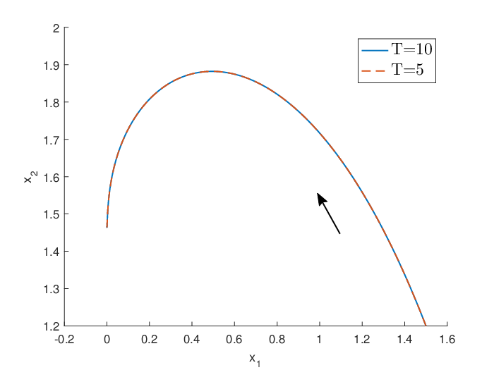
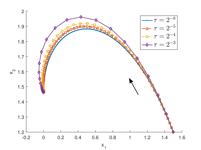
Example 3: Convergence of dynamics under Eckhardt surface. In this example we aim to observe the numerical convergence of dynamics for HiSD. As the exact dynamics of HiSD is not available in practice, we approximate it by the numerical solutions under the very fine mesh size τ=2−8\tau=2^{-8}. The initial conditions are given as

x⁡(0)=(1.5,1.2)⊤,v⁡(0)=15​(−1,2)⊤.x(0)=(1.5,1.2)^{\top},~~v(0)=\frac{1}{\sqrt{5}}(-1,2)^{\top}.

Figure 1(Left) indicates that the HiSD reaches a saddle point under both T=10T=10 and T=5T=5 and thus it suffices to take T=5T=5. Figure 1(Right) shows that not only the saddle point could be achieved under different step sizes, but the dynamics of HiSD globally converges to the exact one (i.e. the curve under τ=2−8\tau=2^{-8}) as the step size τ\tau decreases. These observations justify the theoretical results and demonstrate that the proposed schemes are appropriate methods in computing the dynamic pathways for constructing the solution landscapes, e.g., [13, 26, 30].
Refer to caption
Refer to caption
Fig. 1: (Left) Numerical solution of x⁡(t)x(t) with τ=2−8\tau=2^{-8} and different terminal time TT; (Right) Numerical solution of x⁡(t)x(t) with T=5T=5 and different τ\tau. The symbols on the curves indicate the time steps.

6 Extension to generalized high-index saddle dynamics for dynamical systems

In many autonomous dynamical systems x˙=F⁡(x)\dot{x}=F(x), the force F⁡(x)F(x) is not derived from the variation of some energy function/functional E⁡(x)E(x), which does not follow the formulations of the HiSD proposed in Section 2. In this case, the following GHiSD was developed in [30] to compute the high-index saddle points for non-gradient systems:

{d​xd​t=(I−2​∑j=1kvj​vj⊤)​F​(x),d​vid​t=(I−vivi⊤)J~(x)vi−∑j=1i−1vjvj⊤(J~(x)+J~⊤(x))vi,1≤i≤k.\left\{\begin{array}[]{l}\displaystyle\frac{dx}{dt}=\bigg(I-2\sum_{j=1}^{k}v_{j}v_{j}^{\top}\bigg)F(x),\\[5.42003pt] \displaystyle\frac{dv_{i}}{dt}=(I-v_{i}v_{i}^{\top})\tilde{J}(x)v_{i}-\sum_{j=1}^{i-1}v_{j}v_{j}^{\top}(\tilde{J}(x)+\tilde{J}^{\top}(x))v_{i},~~1\leq i\leq k.\end{array}\right. (41)

Here J~\tilde{J} refers to the Jacobian of FF, which is in general not symmetric. Compared with the high-index saddle dynamics (1), which works for the gradient systems with the symmetric Hessian J⁡(x)J(x), J~​(x)+J~⊤​(x)\tilde{J}(x)+\tilde{J}^{\top}(x) is used to replace 2​J​(x)2J(x) in the dynamics of {vi}i=1k\{v_{i}\}_{i=1}^{k}.

Similar to (27), we could propose the explicit Euler scheme of (41) for 1≤n≤NT1\leq n\leq N_{T} as follows

{xn=xn−1+τ⁡(I−2​∑j=1kvj,n−1​vj,n−1⊤)​F​(xn−1),v~i,n=vi,n−1+τ⁡(I−vi,n−1​vi,n−1⊤)​J~​(xn−1)​vi,n−1−∑j=1i−1vj,n−1vj,n−1⊤(J~(xn−1)+J~⊤(xn−1))vi,n−1,1≤i≤k,vi,n=1Yi,n(v~i,n−∑j=1i−1(v~i,n⊤vj,n)vj,n),1≤i≤k.\left\{\begin{array}[]{l}\displaystyle x_{n}=x_{n-1}+\tau\bigg(I-2\sum_{j=1}^{k}v_{j,n-1}v_{j,n-1}^{\top}\bigg)F(x_{n-1}),\\[7.22743pt] \displaystyle\tilde{v}_{i,n}=v_{i,n-1}+\tau\big(I-v_{i,n-1}v_{i,n-1}^{\top}\big)\tilde{J}(x_{n-1})v_{i,n-1}\\[7.22743pt] \displaystyle\hskip 50.58878pt-\sum_{j=1}^{i-1}v_{j,n-1}v_{j,n-1}^{\top}\big(\tilde{J}(x_{n-1})+\tilde{J}^{\top}(x_{n-1})\big)v_{i,n-1},~~1\leq i\leq k,\\ \displaystyle v_{i,n}=\frac{1}{Y_{i,n}}\bigg(\displaystyle\tilde{v}_{i,n}-\sum_{j=1}^{i-1}(\tilde{v}_{i,n}^{\top}v_{j,n})v_{j,n}\bigg),~~1\leq i\leq k.\end{array}\right. (42)

Intuitively, we may extend the developed methods and results in previous sections to GHiSD (41) for non-gradient systems. Although there are differences between (1) and (41) as mentioned above, we notice that the derivations could be performed similarly. After carefully checking the preceding estimates, a key step lies in the quantification of v~m,n⊤​v~i,n\tilde{v}_{m,n}^{\top}\tilde{v}_{i,n} in (28). We thus calculate this product for m<im<i for the case of generalized saddle dynamics (41) as follows

v~m,n⊤v~i,n=[vm,n−1+τ(I−vm,n−1vm,n−1⊤)J~(xn−1)vm,n−1−τ∑j=1m−1vj,n−1vj,n−1⊤(J~(xn−1)+J~⊤(xn−1))vm,n−1]⊤[vi,n−1+τ(I−vi,n−1vi,n−1⊤)J~(xn−1)vi,n−1−∑j=1i−1vj,n−1vj,n−1⊤(J~(xn−1)+J~⊤(xn−1))vi,n−1]=τ⁡(vm,n−1⊤​J~​(xn−1)​vi,n−1+vm,n−1⊤​J~⊤​(xn−1)​vi,n−1CLOSEOPEN−vm,n−1⊤​(J~​(xn−1)+J~⊤​(xn−1))​vi,n−1)+τ2​[⋯]=τ2​[⋯],\begin{array}[]{l}\displaystyle\tilde{v}_{m,n}^{\top}\tilde{v}_{i,n}=\bigg[v_{m,n-1}+\tau\big(I-v_{m,n-1}v_{m,n-1}^{\top}\big)\tilde{J}(x_{n-1})v_{m,n-1}\\[10.84006pt] \displaystyle\qquad\qquad\qquad-\tau\sum_{j=1}^{m-1}v_{j,n-1}v_{j,n-1}^{\top}\big(\tilde{J}(x_{n-1})+\tilde{J}^{\top}(x_{n-1})\big)v_{m,n-1}\bigg]^{\top}\\[10.84006pt] \displaystyle\qquad\qquad\quad\bigg[v_{i,n-1}+\tau\big(I-v_{i,n-1}v_{i,n-1}^{\top}\big)\tilde{J}(x_{n-1})v_{i,n-1}\\[10.84006pt] \displaystyle\qquad\qquad\qquad-\sum_{j=1}^{i-1}v_{j,n-1}v_{j,n-1}^{\top}\big(\tilde{J}(x_{n-1})+\tilde{J}^{\top}(x_{n-1})\big)v_{i,n-1}\bigg]\\[10.84006pt] \displaystyle\qquad\quad~=\tau\big(v_{m,n-1}^{\top}\tilde{J}(x_{n-1})v_{i,n-1}+v_{m,n-1}^{\top}\tilde{J}^{\top}(x_{n-1})v_{i,n-1}\\[7.22743pt] \displaystyle\qquad\qquad\qquad-v_{m,n-1}^{\top}\big(\tilde{J}(x_{n-1})+\tilde{J}^{\top}(x_{n-1})\big)v_{i,n-1}\big)+\tau^{2}[\cdots]=\tau^{2}[\cdots],\end{array}

where we used the fact that

vm,n−1⊤​J~​(xn−1)​vi,n−1+vm,n−1⊤​J~⊤​(xn−1)​vi,n−1−vm,n−1⊤​(J~​(xn−1)+J~⊤​(xn−1))​vi,n−1=0.\begin{array}[]{l}\displaystyle v_{m,n-1}^{\top}\tilde{J}(x_{n-1})v_{i,n-1}+v_{m,n-1}^{\top}\tilde{J}^{\top}(x_{n-1})v_{i,n-1}\\[3.61371pt] \displaystyle\qquad\qquad\qquad-v_{m,n-1}^{\top}\big(\tilde{J}(x_{n-1})+\tilde{J}^{\top}(x_{n-1})\big)v_{i,n-1}=0.\end{array}

Note that this nice property stems from the symmetrization J~​(x)+J~⊤​(x)\tilde{J}(x)+\tilde{J}^{\top}(x) in the GHiSD (41). By virtue of this symmetrization, we could derive the error estimates for explicit Euler scheme (42) in parallel with the proofs in previous sections, and thus show the numerical accuracy of GHiSD (41) for non-gradient systems.

7 Conclusions

In this paper we develop novel techniques to overcome the strong nonlinearity and the difficulties caused by the orthonormalization procedure to prove error estimates for Euler discretization of HiSD with respect to the time step size, which serves as an important compensation for the gap between the continuous problem and the numerical implementation. The developed methods and results are further extended to study the GHiSD for non-gradient systems, and thus provide theoretical supports for the accuracy of numerical computations.

There are several other potential extensions of the current work. For instance, the ideas and techniques could be employed and improved to analyze implicit schemes or high-order methods like the backward difference formulas of HiSD in order to retain high-order accuracy. How to relax the linearly growth and Lipschitz conditions on the force FF and the Hessian JJ (or Jacobian in non-gradient systems) in the error estimates is also an important but challenging topic as many energy surfaces do not enjoy these properties. We may further extend the methods to study the numerical schemes of the dimer-type methods such as the shrinking dimer dynamics [33]. However, as the multiplication of the Hessian and the vector is approximated by dimer methods in order to reduce the computational costs, the current Hessian-based proofs do not apply and additional investigations will be carried out in the near future. Recently, a constrained high-index saddle dynamics (CHiSD) was developed to compute high-index saddle points of an energy functional subject to equality constraints [27]. Applying the Riemannian gradients and Hessians, the CHiSD is derived as the dynamical system with a transformed gradient flow. In the numerical implementation, the retraction operator and vector transport are introduced to discretize the CHiSD. Thus, it will be very interesting to study the error estimates for numerical schemes of CHiSD in future.

It is also worth mentioning that in the current work we focus on the dynamics of HiSD on the finite interval t∈[0,T]t\in[0,T] and prove error estimates to show the pathway convergence of numerical solutions of HiSD. For most applications, numerical schemes of HiSD could reach the target saddle point within a certain number of iterations (e.g., the observations in the left plot of Figure 1), and thus the derived error estimate results in this work could apply by setting a suitable TT. Nevertheless, the convergence to the saddle point is theoretically determined by the rate of x⁡(t)→x∗x(t)\rightarrow x_{*} as t→∞t\rightarrow\infty, thus it is desirable to perform the error estimate of xn−x∗x_{n}-x_{*} for n→∞n\rightarrow\infty as in the literature of optimization algorithms [17, 23]. In a very recent work [19] the convergence analysis of HiSD is performed to determine the convergence rate of xn−x∗x_{n}-x_{*} for n→∞n\rightarrow\infty. It should be pointed out that the result in the current work that v1,n−v1​(tn)v_{1,n}-v_{1}(t_{n}) has the first-order accuracy with respect to the time step size was borrowed in [19] in order to prove the approximation of eigenvector, which again shows the importance of novel techniques proposed in this work.

Acknowledgements

This work was partially supported by the National Key Research and Development Program of China 2021YFF1200500; the National Natural Science Foundation of China No. 12050002 and 21790340; the International Postdoctoral Exchange Fellowship Program No. YJ20210019; the China Postdoctoral Science Foundation Nos. 2021TQ0017 and 2021M700244.

References

  • [1] J. Baker, An algorithm for the location of transition states. J. Comput. Chem., 7 (1986), 385–395.
  • [2] H. Brunner, Collocation methods for Volterra integral and related functional differential equations. Cambridge University Press, Cambridge, 2004.
  • [3] J. Doye and D. Wales, Saddle points and dynamics of Lennard-Jones clusters, solids, and supercooled liquids. J Chem Phys 116 (2002), 3777–3788.
  • [4] B. Eckhardt, Irregular scattering. Phys. D 33 (1988), 89–98.
  • [5] W. E, E. Vanden-Eijnden, Transition-path theory and path-finding algorithms for the study of rare events, Annu. Rev. Phys. Chem., 61 (2010), 391-420.
  • [6] W. E and X. Zhou, The gentlest ascent dynamics. Nonlinearity 24 (2011), 1831–1842.
  • [7] P. E. Farrell, Á. Birkisson, and S. W. Funke, Deflation Techniques for Finding Distinct Solutions of Nonlinear Partial Differential Equations. SIAM J. Sci. Comput. 37 (2015), A2026–A2045.
  • [8] W. Gao, J. Leng, and X. Zhou, An iterative minimization formulation for saddle point search. SIAM J. Numer. Anal. 53 (2015), 1786–1805.
  • [9] I. Goodfellow, Y. Bengio, A. Courville, Deep learning. The MIT Press, Cambridge, MA, 2016.
  • [10] N. Gould, C. Ortner and D. Packwood, A dimer-type saddle search algorithm with preconditioning and linesearch. Math. Comp. 85 (2016), 2939–2966.
  • [11] Y. Han, Y. Hu, P. Zhang, A. Majumdar, L. Zhang, Transition pathways between defect patterns in confined nematic liquid crystals. J. Comput. Phys. 396 (2019), 1–11.
  • [12] Y. Han, Z. Xu, A. Shi, L. Zhang, Pathways connecting two opposed bilayers with a fusion pore: a molecularly-informed phase field approach. Soft Matter 16 (2020), 366–374.
  • [13] Y. Han, J. Yin, P. Zhang, A. Majumdar, L. Zhang, Solution landscape of a reduced Landau–de Gennes model on a hexagon. Nonlinearity 34 (2021), 2048–2069.
  • [14] Y. Han, J. Yin, Y. Hu, A. Majumdar, L. Zhang, Solution landscapes of the simplified Ericksen-Leslie model and its comparison with the reduced Landau-de Gennes model, Proceedings of the Royal Society A, 477 (2021), 20210458.
  • [15] G. Henkelman, H. Jónsson, A dimer method for finding saddle points on high dimensional potential surfaces using only first derivatives. J. Chem. Phys. 111 (1999), 7010–7022.
  • [16] A. Levitt and C. Ortner, Convergence and cycling in walker-type saddle search algorithms. SIAM J. Numer. Anal. 55 (2017), 2204–2227.
  • [17] C. Li, M. Wang, H. Liu, T. Zhang, Near-optimal stochastic approximation for online principal component estimation. Math. Program. 167 (2018), 75–97.
  • [18] , Y. Li and J. Zhou, A minimax method for finding multiple critical points and its applications to semilinear PDEs, SIAM J. Sci. Comput. 23 (2001), 840–865.
  • [19] Y. Luo, X. Zheng, X. Cheng, L. Zhang, Convergence analysis of discrete high-index saddle dynamics. arXiv:2204.00171.
  • [20] D. Mehta, Finding all the stationary points of a potential-energy landscape via numerical polynomial-homotopy-continuation method, Phys Rev E 84 (2011) 025702.
  • [21] J. W. Milnor, Morse Theory, Princeton University Press, 1963.
  • [22] R. M. Minyaev, W. Quapp, G. Subramanian, P. R. Schleyer, Y. Ho, Internal conrotation and disrotation in H2BCH2BH2 and diborylmethane 1, 3 H exchange. J. Comput. Chem. 18 (1997), 1792–1803.
  • [23] Y. Nesterov, Introductory lectures on convex optimization: A basic course. Applied Optimization, 87. Kluwer Academic Publishers, Boston, MA, 2004.
  • [24] W. Wang, L. Zhang, P. Zhang, Modelling and computation of liquid crystals. Acta Numerica 30 (2021), 765–851.
  • [25] X. Xu, C. L. Ting, I. Kusaka, Z. G. Wang, Nucleation in polymers and soft matter. Annu. Rev. Phys. Chem., 65 (2014), 449-475.
  • [26] Z. Xu, Y. Han, J. Yin, B. Yu, Y. Nishiura, L. Zhang, Solution landscapes of the diblock copolymer-homopolymer model under two-dimensional confinement. Phys. Rev. E 104 (2021), 014505.
  • [27] J. Yin, Z. Huang, L. Zhang, Constrained high-index saddle dynamics for the solution landscape with equality constraints, J. Sci. Comput. to appear.
  • [28] J. Yin, K. Jiang, A.-C. Shi, P. Zhang, L. Zhang, Transition pathways connecting crystals and quasicrystals, Proc. Natl. Acad. Sci. U.S.A. 118 (2021), e2106230118.
  • [29] J. Yin, Y. Wang, J. Chen, P. Zhang, L. Zhang, Construction of a pathway map on a complicated energy landscape. Phys. Rev. Lett. 124 (2020), 090601.
  • [30] J. Yin, B. Yu, L. Zhang, Searching the solution landscape by generalized high-index saddle dynamics. Sci. China Math. 64 (2021), 1801.
  • [31] J. Yin, L. Zhang, P. Zhang, High-index optimization-based shrinking dimer method for finding high-index saddle points. SIAM J. Sci. Comput. 41 (2019), A3576–A3595.
  • [32] J. Yin, L. Zhang, P. Zhang, Solution landscape of Onsager functional identifies non-axisymmetric critical points, Physica D: Nonlinear Phenomena 430 (2022), 133081.
  • [33] J. Zhang, Q. Du, Shrinking dimer dynamics and its applications to saddle point search. SIAM J. Numer. Anal. 50 (2012), 1899–1921.
  • [34] L. Zhang, W. Ren, A. Samanta, Q. Du, Recent developments in computational modelling of nucleation in phase transformations. npj Comput. Mater. 2 (2016), 16003.
  • [35] L. Zhang, L. Chen, Q. Du, Morphology of critical nuclei in solid-state phase transformations. Phys. Rev. Lett. 98 (2007), 265703.
  • [36] L. Zhang, L. Chen, Q. Du, Simultaneous prediction of morphologies of a critical nucleus and an equilibrium precipitate in solids. Commun. Comput. Phys. 7 (2010), 674–682.
  • [37] L. Zhang, Q. Du, Z. Zheng, Optimization-based shrinking dimer method for finding transition states. SIAM J. Sci. Comput. 38 (2016), A528–A544.