Entanglement entropy in the Ising model with topological defects

Entanglement plays a central role in the development of long-range correlations in quantum critical phenomena. Thus, quantification of the entanglement in a quantum-critical system provides a way to characterize the universal properties of the critical point. The von-Neumann entropy is a natural candidate to perform this task. For zero-temperature ground-states of 1+1D quantum-critical systems described by conformal field theories (CFTs), the von-Neumann entropy [equivalently, entanglement entropy (EE)] for a subsystem exhibits universal logarithmic scaling with the subsystem size Holzhey et al. 1994; Calabrese and Cardy 2004. The coefficient of this scaling determines a fundamental property of the bulk CFT: the central charge. For finite systems with boundaries at a conformal critical point, the EE receives universal, subleading, boundary-dependent contributions, the so-called ‘boundary entropy’ Affleck and Ludwig 1991 – a central concept in a variety of physical problems both in condensed matter physics and string theory. This boundary contribution to the EE provides a valuable diagnostic for identifying the different boundary fixed points of a given CFT Calabrese and Cardy 2004; Calabrese and Cardy 2009; Affleck et al. 2009; Roy et al. 2020; Roy et al. 2021.

While entanglement has been analyzed extensively in CFTs with and without boundaries, its behavior is much less understood in the presence of defects. The question is particularly intriguing since entanglement measures may provide an alternate way to classify defects in CFTs. Of particular interest are topological (perfectly-transmissive) defects Petkova and Zuber 2001; Bachas et al. 2002; Fröhlich et al. 2004; Frohlich et al. 2007; Aasen et al. 2016. These defects commute with the generators of conformal transformations and thus, can be deformed without affecting the values of the correlation functions as long as they are not taken across field insertions (hence the moniker topological). They reflect the internal symmetries of the CFT and relate the order-disorder dualities of the CFT to the high-low temperature dualities of the corresponding off-critical model Fröhlich et al. 2004; Kramers and Wannier 1941; Savit 1980. They also play an important role in the study of anyonic chains and in the correspondence between CFTs and three-dimensional topological field theories Buican and Gromov 2017.

It is natural to analyze EE in the presence of topological defects. Two distinct geometries have been considered in the literature: i) where the defect is entirely within the subsystem, and ii) where the defect is located precisely at the interface between the subsystem and the rest. While both cases exhibit identical leading-order logarithmic scaling with subsystem size, they differ when subleading, i.e., $O(1)$, corrections are taken into account. In the first case, after usual folding maneuvers, the subleading term can be equated to a boundary entropy with double the bulk degrees of freedom Oshikawa and Affleck 1997; Saleur 1998; Saleur 2000. In this way, the subleading correction to symmetric EE can be computed analytically for all rational CFTs Gutperle and Miller 2016. In the second case, the subleading term for the interface EE is much more difficult to obtain. Field-theory computations based on the replica trick for the free, real boson Sakai and Satoh 2008, the free, real fermion Brehm and Brunner 2015 (see also Eisler and Peschel 2010; Peschel and Eisler 2012; Calabrese et al. 2012) and generalization to all rational CFTs Gutperle and Miller 2016 using the corresponding twisted torus partition functions Petkova and Zuber 2001 provide results whose validity have never been tested with ab-initio, lattice computations. Such a computation is particularly important since the mapping to the twisted torus partition function does not faithfully capture the geometric arrangement of the subsystem with respect to the defect. This is important for subleading terms in the interface EE which are, in fact, the signatures of the topological defect.

Our goal, in this paper, is to investigate the question in the simplest possible case, the Ising model, using ab-initio calculations. These calculations are more complex than is usually the case for EE due to the presence of zero-energy modes. The latter are a salient feature of the topological nature of the defect. While the effects of zero-modes have been extensively quantified in gapped systems due to their relevance in topologically ordered systems, the same is much less understood in the critical systems. Here, we show that these zero-modes give rise to nontrivial contributions to the EE when the subsystem size is comparable to the size of the whole system, similar to the case of a periodic ring of free fermions Herzog and Nishioka 2013; Klich et al. 2017. Thus, these zero-modes profoundly affect corrections to scaling. After the role of these zero-modes is properly taken into account, we find results that are as expected for case (i), but are not compatible with the formulas proposed in the string/field theory literature Brehm and Brunner 2015; Gutperle and Miller 2016 for case (ii).

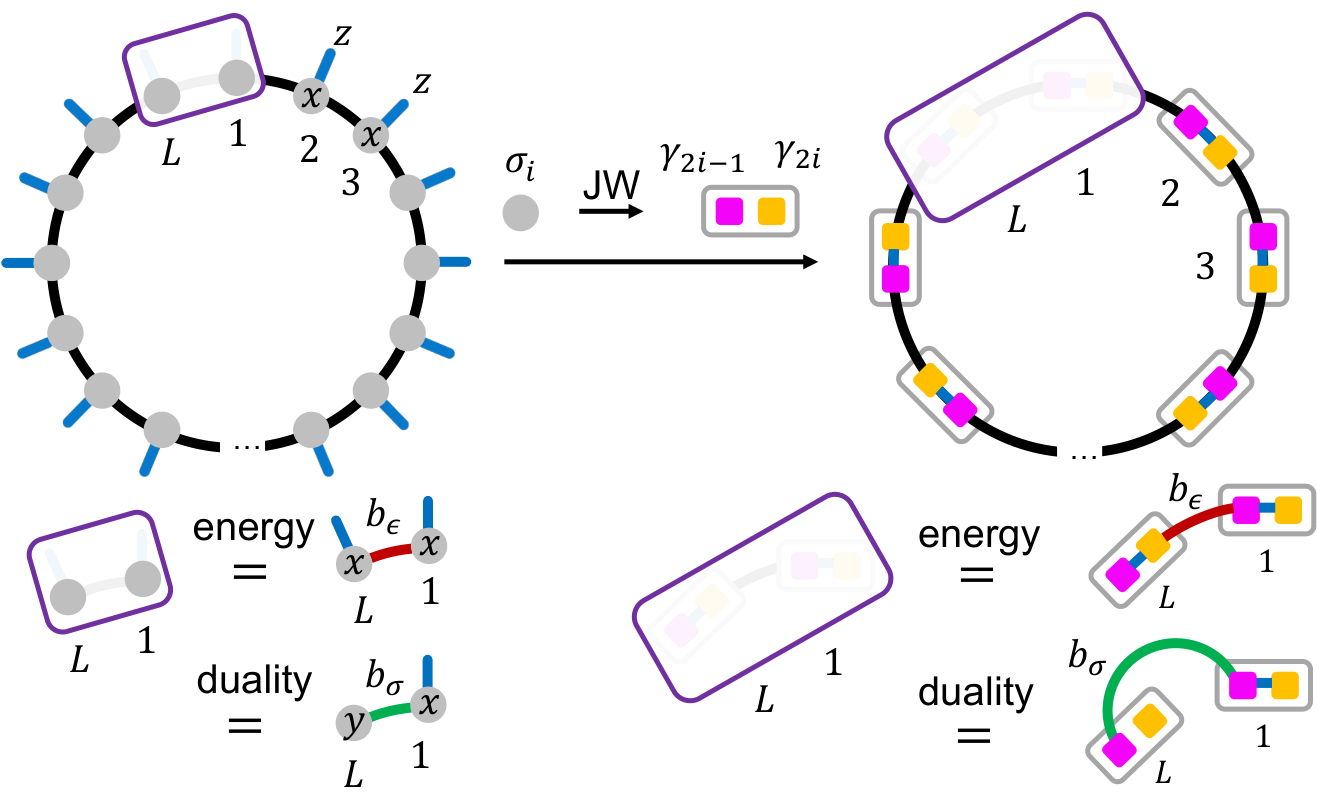
The Ising model provides a particularly appropriate testbed for the EE in the presence of topological defects due to the following. First, the lattice Hamiltonians are well-understood Grimm 2002; Oshikawa and Affleck 1997. Second, the zero-mode structure is the simplest and yet, sufficient to explain the main concepts. Third, the defect Hamiltonian can be mapped, after Jordan-Wigner (JW) transformation, to a bilinear fermionic Hamiltonian. The latter can be diagonalized semi-analytically and leads to very accurate predictions of EE Vidal et al. 2003; Peschel 2003; Latorre et al. 2004. To emphasize the nontrivial nature of the topological defect, we compare our results with the non-topological defects in the model.

There are two nontrivial classes of defects in the Ising CFT: energy ($\epsilon$) and duality ($\sigma$). We consider a periodic Ising chain with the defect concerning the spins at sites $L$ and 1 Henkel et al. 1989; Baake et al. 1989; Grimm 2002. The Hamiltonians are: $H_{\epsilon,\sigma}=H_{0}$$-h_{\epsilon,\sigma}$ (see Fig. 1). Here, the bulk Hamiltonian term, $H_{0},=-\sum_{i=1}^{L-1}\sigma_{i}^{x}\sigma_{i+1}^{x}/2$ $-\sum_{i=1}^{L-1}\sigma_{i}^{z}/2$. The two defect terms are: $h_{\epsilon}=b_{\epsilon}\sigma_{L}^{x}\sigma_{1}^{x}/2$ $+\sigma_{L}^{z}/2$ and $h_{\sigma}=b_{\sigma}\sigma_{L}^{y}\sigma_{1}^{x}/2$ ¹¹ 1 Note that $h_{\epsilon,\sigma}$ are marginal perturbations which, in general, lead to continuously varying critical exponents Cardy 1987.. The energy defect consists of one bond with altered strength $b_{\epsilon}$ connecting spins at sites $L$ and 1. In particular, $b_{\epsilon}=0,+1$ and $-1$ correspond to Ising models with open, periodic and antiperiodic boundary conditions (bcs) respectively. Unlike the energy defect, the duality defect consists of a $\sigma_{L}^{y}\sigma_{1}^{x}$ interaction ²² 2 This duality defect Hamiltonian is related by a local unitary rotation on the $L^{\rm th}$ spin to the one considered in Refs. Oshikawa and Affleck 1997, which has $\sigma_{L}^{z}\sigma_{1}^{x}$ interaction. We do not use this alternate form since it no longer leads to a bilinear Hamiltonian under JW transformation and cannot be solved by free-fermion techniques. . Equally important, there is no transverse field at the $L^{\rm th}$ site. The duality defect for $b_{\sigma}=1$ (equivalently $b_{\sigma}=-1$, which is related by a local unitary rotation) is the topological defect for the Ising CFT.

Next, we perform a JW transformation: $\gamma_{2k-1}=\sigma_{k}^{x}\prod_{j=1}^{k-1}\sigma_{j}^{z}$, $\gamma_{2k}=\sigma_{k}^{y}\prod_{j=1}^{k-1}\sigma_{j}^{z}$, where $\gamma_{j}$-s are real, Majorana fermion operators obeying $\{\gamma_{j},\gamma_{k}\}=2\delta_{j,k}$. In the fermionic language, the defect Hamiltonians are $H_{\epsilon,\sigma}^{f}=H_{0}^{f}-h_{\epsilon,\sigma}^{f}$, where

Here we have restricted ourselves to the symmetry sector $Q=\prod_{j=1}^{L}\sigma_{j}^{z}=1$ ³³ 3 Equivalently, we analyze the mixed sector Hamiltonian Grimm 2002: $H_{\epsilon,\sigma}^{m}=P_{+}H_{\epsilon,\sigma}^{f}(Q=+1)+P_{-}H_{\epsilon,\sigma}^{f}(Q=-1)$. For the energy defect, from the definition of $H_{\epsilon}^{f}$, we recover the well-known fact that the periodic (antiperiodic) coupling at the boundary for the spin model corresponds to antiperiodic (periodic) coupling for the fermionic model. In particular, the periodic fermionic model ($b_{\epsilon}=-1$) contains two nonlocal Majorana zero-modes, which together are responsible for the two-fold degenerate ground-state of the fermionic model. For the duality defect, the operator $\gamma_{2L}$ does not occur in $H_{\sigma}^{f}$. It commutes with the Hamiltonian: $[\gamma_{2L},H_{\sigma}^{f}]=0$, and anticommutes with the conserved $\mathbb{Z}_{2}$ charge: $\{\gamma_{2L},Q\}=0$. Thus, it is a zero-mode of the model which is perfectly localized in space. It has a partner zero-mode which is completely delocalized: $\Lambda(b_{\sigma})=\sum_{k=1}^{L}\gamma_{2k-1}+b_{\sigma}\sum_{k=1}^{L-1}\gamma_{2k}$. Note that the zero-modes exist for all values of $b_{\sigma}$ and are not special features of the topological point. The fermionic Hamiltonian also reaffirms a CFT result Grimm 2002: $H_{\sigma}^{f}$ describes a chain of $2L-1$ Majorana fermions or equivalently, $L-1/2$ spins. This is important for quantifying finite-size effects.

Now, we compute symmetric and interface EEs for the ground states of the fermionic Hamiltonians $H_{\epsilon,\sigma}^{f}$. Since the latter are bilinear in the fermionic operators, we compute the relevant EEs from the ground-state correlation matrix Vidal et al. 2003; Peschel 2003; Latorre et al. 2004. The latter is calculated from the ground state by filling up the negative energy states. The method is unambiguous in the absence of zero-energy modes. However, in the presence of the latter (e.g., $b_{\epsilon}=-1$ or any $b_{\sigma}$), it raises the question: are the zero-energy states empty or occupied in the ground state? Yet another possibility is to consider an incoherent superposition of filled and empty states. This leads to the total system being in a mixed state, but is appropriate when taking the zero-temperature limit of a thermal ensemble Herzog and Nishioka 2013. The question is crucial to the computation since zero-energy modes nontrivially affect the EE. For $b_{\epsilon}=-1$, the zero-modes give rise to nontrivial corrections to the EE of a subsystem of size $r$ within a total system of size $L$ Herzog and Nishioka 2013; Klich et al. 2017. The correction $\Delta S(r/L)=$ $\frac{\pi r}{L}\int_{0}^{\infty}\tanh(\pi rh/L)[\coth(\pi h)-1]$. For $r\ll L$, the EE is oblivous to the existence of the two nonlocal zero-modes spread throughout the system: $\Delta S\simeq\pi^{2}r^{2}/12L^{2}\rightarrow 0$. The situation changes as the subsystem occupies appreciable fraction of the total system ($r\sim L$) culminating in $\Delta S(r=L)=\ln 2$, the latter being the entropy of the two-fold degenerate ground state of a periodic chain of fermions. Below, we present analogous results for the topological defect considering separately the cases when the total system is in a pure and mixed state for the relevant fermionic models ⁴⁴ 4 See Supplementary Material for details.

First, we compute the symmetric EE (Fig. 2). The results for $b_{\epsilon}=1$ (no defect) are shown with blue crosses. The symmetric EE exhibits the expected logarithmic scaling: $S_{s}(b_{\epsilon}=1)$ $=\frac{c}{3}\ln\big[\frac{L}{\pi}\sin\big(\frac{\pi r}{L}\big)\big]$ $+S_{0}$ for all values of $r/L$. We set the lattice spacing to 1 throughout this work. Fitting this expression yields the expected central charge $c\simeq 0.5$ and $S_{0}\simeq 0.478$. The maroon (green) hexagons corresponds to the symmetric EE for $b_{\epsilon}=-1$ ($b_{\sigma}=1$) when the total system is in an incoherent superposition of the zero-energy states being filled and empty. Compared to $S_{s}(b_{\epsilon}=1)$, the symmetric EEs ($S_{s}^{m},m$ denoting the total system being mixed) for the two cases get an additional contribution of $\Delta S(r/L)$ Klich et al. 2017 and $\Delta S(r/L)/2+(\ln 2)/2$. Thus, when $r/L\ll 1$, for both $b_{\epsilon}=-1$ and $b_{\sigma}=1$, $S_{s}^{m}$ exhibits the expected logarithmic dependence with $c\simeq 0.5$ (left panel). However, the offset, $S_{0}$, for $S_{s}^{m}(b_{\sigma}=1)$ is $(\ln 2)/2$ higher. This higher offset unambiguously distinguishes the topological defect from the energy defect and is because of the localized unpaired Majorana zero mode at the center of the subsystem (the result will be the same as long as the defect lies within and not at the edge of the subsystem). This is consistent with the identification of this defect problem to a boundary CFT problem at the ‘continuous Neumann boundary fixed-point’ after folding, with the corresponding $g$-function $=\sqrt{2}$ Oshikawa and Affleck 1997 (see also Ref. Alba et al. 2017). This should be compared with the ‘continuous Dirichlet boundary fixed point’ ($b_{\epsilon}=-1$ case), which has $g$-function $=1$ and thus, no additional boundary entropy contribution. For $b_{\sigma}=1$, increasing $r/L$ leads to a further offset of $\Delta S(r/L)/2$ due to the contribution from the second nonlocal zero-mode. Here, the factor of 1/2 accounts for the difference in the number of nonlocal zero-modes in the $b_{\epsilon}=-1$ and $b_{\sigma}=1$ models. The maroon squares (green diamonds) correspond to the symmetric EEs obtained by keeping the zero-energy state empty (denoted by $S_{s}^{p},p$ denoting the total system being pure; the results are identical for the filled case). Now, the results for $b_{\epsilon}=\pm 1$ are indistinguishable. However, compared to the case without defects, $S_{s}^{p}(b_{\sigma}=1)$ exhibits a $\Delta S(1-r/L)/2$ offset. For $r\ll L$, this again leads to the offset, $S_{0}$, being $(\ln 2)/2$ higher than the other cases. For $r\sim L$, the $S_{s}^{p}$ diminishes compared to the case when the total system is mixed due to the purity of the total system.

Next, we compute the interface EE (Fig. 3), where one end of the subsystem (of size $r$) is located at the defect and the other end sweeps through the system (of size $L$) ⁵⁵ 5 Note that the symmetric EE computation required much larger total system sizes in order to get a good result for offset $(\ln 2)/2$.. For $b_{\epsilon}=-1$, the results are identical to the symmetric case. This is expected since the resulting model is just a fermionic model with periodic bc and there is no difference between symmetric and interface EEs. The results for $b_{\sigma}=1$ are the same for the total system in a mixed (green hexagons) and pure (green diamonds) state. Then, $S_{\cal I}^{m,p}(b_{\sigma}=1)$ is given by the EE of an Ising chain of length $L-1/2$ without any defects [$S_{{\cal I},L-1/2}(b_{\epsilon}=1)$] together with an offset. The first contribution to this offset is $\Delta S[r/(L-1/2)]$. It arises as the subsystem size grows and becomes aware of the nonlocal zero-mode $\Lambda(b_{\sigma})$ in the chain of length $L-1/2$. The second contribution, $\delta_{r,L}(\ln 2)/2$, arises only when $r=L$. This is due the localized zero-mode, $\gamma_{2L}$, which contributes only when the subsystem covers the entire system. The resulting prediction is shown with orange pluses. For comparison, we have also shown the curves obtained by computing the corresponding offsets for the system-size $L$ (green pluses). For $r$ not close to $L$, both predictions work well. However, for $L-r\sim 1$, only the computation with system-size $L-1/2$ leads to the correct predictions (see inset). The field-theory computations are usually done for $1\ll r,L$ with $r$ not too close to $L$. For definiteness, we consider the scaling of $S_{\cal I}(r=L/2)$ with $\ln L$ Gutperle and Miller 2016; Brehm and Brunner 2015. Fitting to $S_{\cal I}(r=L/2)=(c/3)\ln L+\tilde{S}_{0}$ ⁶⁶ 6 Note that for a periodic (open) system, the coefficient of $\ln L$ is $c/3$ $(c/6)$. yields the expected central charge $c\simeq 0.5$ for all the curves. Recall that for $0\leq b_{\sigma}<1$, the coefficient of $\ln L$ is $c_{\rm eff}/3$, where the ‘effective central charge’ $c_{\rm eff}\in[0,1/2)$ Eisler and Peschel 2010; Brehm and Brunner 2015. The difference of the offsets, $\tilde{S}_{0}$, between $b_{\epsilon}=-1$ and $b_{\epsilon}=1$ cases is $2\Delta_{I}=\Delta S(1/2)$ $=-1/2+\ln 2$ or 0 depending on the total system being in a mixed or pure state. For the topological case, both pure and mixed states, the corresponding offset difference is $\Delta_{I}=\Delta S(1/2)/2=-1/4+(\ln 2)/2$. Importantly, this offset occurs entirely due to a ‘finite-size effect’ correction arising due to the existence of nonlocal zero-modes and bears no relationship to the specific modular S-matrix elements predicted in Refs. Gutperle and Miller 2016; Brehm and Brunner 2015.

To summarize, we computed the symmetric and interface EEs for the Ising CFT with a topological defect taking into account the subtle effects of the zero-modes on the EEs. We showed that while both the EEs exhibit identical leading-order logarithmic scaling, the subleading $O(1)$ corrections are of completely different origin. The subleading term [$=(\ln 2)/2$] for the symmetric EE is related to the $g$-function of the corresponding defect at the boundary in the folded picture. However, the corresponding term [$\Delta S(r/L)/2$] in the interface EE arises only when the subsystem occupies a finite fraction of the total system and is entirely due to the local and nonlocal zero-modes of the topological defect Hamiltonian. In the limit $r\ll L$, there is no additional offset compared with the case without defect. The interface EE result is in sharp contrast with the existing predictions in terms of the modular S-matrix of the CFT Brehm and Brunner 2015; Gutperle and Miller 2016, which predict an offset equal to $-\ln 2$ instead. We also computed the EEs in the case of open/free boundary conditions with a defect at the center of the chain ⁷⁷ 7 See Supplementary Material for details. The results for symmetric EE were identical to that obtained for the periodic chain. The offset interface EE is the same as for the periodic chain when the total system was pure. The total system being mixed contributes another $(\ln 2)/2$ to the offset.

Several features of the topological defect persist away from the topological point, i.e., $b_{\sigma}\neq 1$, and even away from the conformal critical point. We plan to address some of these questions elsewhere. Defect Hamiltonians for other rational CFTs contain more complicated set of zero modes Belletête et al. 2020. The question of subleading corrections in EEs for these models remains open. Finally, advancements in measurement of Renyi entropies in engineered quantum systems Islam et al. 2015; Brydges et al. 2019 and quantum simulation Monroe et al. 2021 can lead to potential verification of our analytical predictions.

We thank Natan Andrei, Pasquale Calabrese, Christopher Herzog and Ingo Peschel for discussions. We also thank David Rogerson and Frank Pollmann for discussions and collaborations on a related project. AR acknowledges support from a grant from the Simons Foundation (825876, TDN). HS was supported by ERC Advanced Grant NuQFT.

References

- Holzhey et al. (1994) C. Holzhey, F. Larsen, and F. Wilczek, Geometric and renormalized entropy in conformal field theory, Nuclear Physics B 424, 443 (1994).
- Calabrese and Cardy (2004) P. Calabrese and J. Cardy, Entanglement entropy and quantum field theory, Journal of Statistical Mechanics: Theory and Experiment 2004, P06002 (2004).
- Affleck and Ludwig (1991) I. Affleck and A. W. W. Ludwig, Universal noninteger “ground-state degeneracy” in critical quantum systems, Phys. Rev. Lett. 67, 161 (1991).
- Calabrese and Cardy (2009) P. Calabrese and J. Cardy, Entanglement entropy and conformal field theory, J. Phys. A42, 504005 (2009), arXiv:0905.4013 [cond-mat.stat-mech] .
- Affleck et al. (2009) I. Affleck, N. Laflorencie, and E. S. Sørensen, Entanglement entropy in quantum impurity systems and systems with boundaries, Journal of Physics A: Mathematical and Theoretical 42, 504009 (2009).
- Roy et al. (2020) A. Roy, F. Pollmann, and H. Saleur, Entanglement Hamiltonian of the 1+1-dimensional free, compactified boson conformal field theory, J. Stat. Mech. 2008, 083104 (2020), arXiv:2004.14370 [cond-mat.stat-mech] .
- Roy et al. (2021) A. Roy, D. Schuricht, J. Hauschild, F. Pollmann, and H. Saleur, The quantum sine-Gordon model with quantum circuits, Nucl. Phys. B 968, 115445 (2021), arXiv:2007.06874 [quant-ph] .
- Petkova and Zuber (2001) V. B. Petkova and J. B. Zuber, Generalized twisted partition functions, Phys. Lett. B 504, 157 (2001), arXiv:hep-th/0011021 .
- Bachas et al. (2002) C. Bachas, J. de Boer, R. Dijkgraaf, and H. Ooguri, Permeable conformal walls and holography, JHEP 06, 027, arXiv:hep-th/0111210 .
- Fröhlich et al. (2004) J. Fröhlich, J. Fuchs, I. Runkel, and C. Schweigert, Kramers-wannier duality from conformal defects, Phys. Rev. Lett. 93, 070601 (2004).
- Frohlich et al. (2007) J. Frohlich, J. Fuchs, I. Runkel, and C. Schweigert, Duality and defects in rational conformal field theory, Nucl. Phys. B 763, 354 (2007), arXiv:hep-th/0607247 .
- Aasen et al. (2016) D. Aasen, R. S. K. Mong, and P. Fendley, Topological Defects on the Lattice I: The Ising model, J. Phys. A 49, 354001 (2016), arXiv:1601.07185 [cond-mat.stat-mech] .
- Kramers and Wannier (1941) H. A. Kramers and G. H. Wannier, Statistics of the two-dimensional ferromagnet. part i, Phys. Rev. 60, 252 (1941).
- Savit (1980) R. Savit, Duality in field theory and statistical systems, Rev. Mod. Phys. 52, 453 (1980).
- Buican and Gromov (2017) M. Buican and A. Gromov, Anyonic Chains, Topological Defects, and Conformal Field Theory, Commun. Math. Phys. 356, 1017 (2017), arXiv:1701.02800 [hep-th] .
- Oshikawa and Affleck (1997) M. Oshikawa and I. Affleck, Boundary conformal field theory approach to the critical two-dimensional ising model with a defect line, Nuclear Physics B 495, 533 (1997).
- Saleur (1998) H. Saleur, Lectures on nonperturbative field theory and quantum impurity problems, (1998), arXiv:cond-mat/9812110 .
- Saleur (2000) H. Saleur, Lectures on nonperturbative field theory and quantum impurity problems: Part 2, (2000), arXiv:cond-mat/0007309 .
- Gutperle and Miller (2016) M. Gutperle and J. D. Miller, A note on entanglement entropy for topological interfaces in RCFTs, JHEP 04, 176, arXiv:1512.07241 [hep-th] .
- Sakai and Satoh (2008) K. Sakai and Y. Satoh, Entanglement through conformal interfaces, JHEP 12, 001, arXiv:0809.4548 [hep-th] .
- Brehm and Brunner (2015) E. M. Brehm and I. Brunner, Entanglement entropy through conformal interfaces in the 2D Ising model, JHEP 09, 080, arXiv:1505.02647 [hep-th] .
- Eisler and Peschel (2010) V. Eisler and I. Peschel, Entanglement in fermionic chains with interface defects, Annalen der Physik 522, 679 (2010).
- Peschel and Eisler (2012) I. Peschel and V. Eisler, Exact results for the entanglement across defects in critical chains, Journal of Physics A: Mathematical and Theoretical 45, 155301 (2012).
- Calabrese et al. (2012) P. Calabrese, M. Mintchev, and E. Vicari, Entanglement Entropy of Quantum Wire Junctions, J. Phys. A 45, 105206 (2012), arXiv:1110.5713 [cond-mat.stat-mech] .
- Herzog and Nishioka (2013) C. P. Herzog and T. Nishioka, Entanglement Entropy of a Massive Fermion on a Torus, JHEP 03, 077, arXiv:1301.0336 [hep-th] .
- Klich et al. (2017) I. Klich, D. Vaman, and G. Wong, Entanglement hamiltonians for chiral fermions with zero modes, Phys. Rev. Lett. 119, 120401 (2017).
- Grimm (2002) U. Grimm, Spectrum of a duality twisted Ising quantum chain, J. Phys. A 35, L25 (2002), arXiv:hep-th/0111157 .
- Vidal et al. (2003) G. Vidal, J. I. Latorre, E. Rico, and A. Kitaev, Entanglement in quantum critical phenomena, Phys. Rev. Lett. 90, 227902 (2003), arXiv:quant-ph/0211074 .
- Peschel (2003) I. Peschel, Calculation of reduced density matrices from correlation functions, Journal of Physics A: Mathematical and General 36, L205 (2003).
- Latorre et al. (2004) J. I. Latorre, E. Rico, and G. Vidal, Ground state entanglement in quantum spin chains, Quantum Inf. Comput. 4, 48 (2004).
- Henkel et al. (1989) M. Henkel, A. Patkós, and M. Schlottmann, The ising quantum chain with defects (i). the exact solution, Nuclear Physics 314, 609 (1989).
- Baake et al. (1989) M. Baake, P. Chaselon, and M. Schlottmann, The ising quantum chain with defects (ii). the so(2n)kac-moody spectra, Nuclear Physics B 314, 625 (1989).
- (33) Note that are marginal perturbations which, in general, lead to continuously varying critical exponents Cardy 1987.
- (34) This duality defect Hamiltonian is related by a local unitary rotation on the spin to the one considered in Refs. Oshikawa and Affleck 1997, which has interaction. We do not use this alternate form since it no longer leads to a bilinear Hamiltonian under JW transformation and cannot be solved by free-fermion techniques.
- (35) Equivalently, we analyze the mixed sector Hamiltonian Grimm 2002: .
- (36) See Supplementary Material for details.
- Alba et al. (2017) V. Alba, P. Calabrese, and E. Tonni, Entanglement spectrum degeneracy and the cardy formula in 1+1 dimensional conformal field theories, Journal of Physics A: Mathematical and Theoretical 51, 024001 (2017).
- (38) Note that the symmetric EE computation required much larger total system sizes in order to get a good result for offset .
- (39) Note that for a periodic (open) system, the coefficient of is .
- (40) See Supplementary Material for details.
- Belletête et al. (2020) J. Belletête, A. M. Gainutdinov, J. L. Jacobsen, H. Saleur, and T. S. Tavares, Topological defects in periodic rsos models and anyonic chains (2020), arXiv:2003.11293 [math-ph] .
- Islam et al. (2015) R. Islam, R. Ma, P. M. Preiss, M. Eric Tai, A. Lukin, M. Rispoli, and M. Greiner, Measuring entanglement entropy in a quantum many-body system, Nature 528, 77 (2015).
- Brydges et al. (2019) T. Brydges, A. Elben, P. Jurcevic, B. Vermersch, C. Maier, B. P. Lanyon, P. Zoller, R. Blatt, and C. F. Roos, Probing rényi entanglement entropy via randomized measurements, Science 364, 260–263 (2019).
- Monroe et al. (2021) C. Monroe, W. Campbell, L.-M. Duan, Z.-X. Gong, A. Gorshkov, P. Hess, R. Islam, K. Kim, N. Linke, G. Pagano, and et al., Programmable quantum simulations of spin systems with trapped ions, Reviews of Modern Physics 93, 10.1103/revmodphys.93.025001 (2021).
- Cardy (1987) J. L. Cardy, Continuously varying exponents and the value of the central charge, Journal of Physics A: Mathematical and General 20, L891 (1987).