Large- Chern insulators: lattice field theory and quantum simulation approaches
to correlation effects in the quantum anomalous Hall effect
Abstract
Four-Fermi quantum field theories in (2+1) dimensions lie among the simplest models in high-energy physics, the understanding of which requires a non-perturbative lattice formulation addressing their strongly-coupled fixed points. These lattice models are also relevant in condensed matter, as they offer a neat playground to explore strong correlations in the quantum anomalous Hall (QAH) effect. We give a detailed description of our multidisciplinary approach to understand the fate of the QAH phases as the four-Fermi interactions are increased, which combines strong-coupling and effective-potential techniques, unveiling a rich phase diagram with large- Chern insulators and Lorentz-breaking fermion condensates. Moreover, this toolbox can be enlarged with recent advances in quantum information science, as we show that tensor-network algorithms based on projected entangled pairs can be used to improve our understanding of the strong-coupling limit. We also present a detailed scheme that uses ultra-cold atoms in optical lattices with synthetic spin-orbit coupling to build quantum simulators of these four-Fermi models. This yields a promising alternative to characterise the strongly-coupled fixed points and, moreover, could also explore real-time dynamics and finite-fermion densities.
I Introduction
One of the main tasks in condensed-matter physics is the prediction and classification of new phases of matter, understanding how they can transform into each other via phase transitions Sachdev 2011. Symmetry has played a key role in this endeavour, Landau 1937; Ginzburg and Landau 1950, since the way in which it breaks can be used to understand many ordering patterns at the microscopic level. Despite decades of intense research, observing how different orderings arise from the same microscopic model, and how they can be described by emerging effective theories that cannot be predicted by simply looking at the individual microscopic constituents Anderson 1972, is still a source of much fascination. This emergence is typically a consequence of the interplay of symmetry and strong inter-particle correlations, the latter being induced by interactions among the microscopic constituents. In condensed matter, these constituents typically correspond to the ions forming the crystal structure and the valence electrons, all of them interacting via Coulomb forces Altland and Simons 2006; Fazekas 1999.
Narrow-band metals have turned out to be a particularly-rich playground for this emergence. Here, the Coulomb interaction between the electrons is screened, and can be approximated by a local four-Fermi term that leads to the Hubbard model, the archetype of strongly-correlated fermions in condensed matter Hubbard 1963. The apparent simplicity of this model is deceptive, as it can host an interaction-induced metal-insulator transition at partial band fillings Imada et al. 1998, which defies the naive band-theory distinction between insulators and conductors. In fact, in the half-filled case, these so-called Mott insulators display anti-ferromagnetic ordering as a consequence of magnetic super-exchange interactions and a phase transition where the spin rotational symmetry is spontaneous broken Anderson 1950; Anderson 1963. Moreover, as one dopes this Mott insulator away from half filling, the interplay of anti-ferromagnetism with the dynamics of the holes has been studied as a fully-electronic mechanism that may account for high- superconductivity Anderson 1987; Lee et al. 2006, as the mobility of holes can release the anti-ferromagnetic singlets, allowing them to condense into the superconductor.
Four-Fermi models have also played an important role at much higher energies, starting with the pioneering work of Enrico Fermi on -decay in nuclei Fermi 1934; Wilson 1968; a precursor to the theory of electroweak interactions in the standard model of particle physics. Four-Fermi terms also appear in the so-called Nambu-Jona-Lasinio (NJL) models Nambu and Jona-Lasinio 1961a; Nambu and Jona-Lasinio 1961b, introduced as a description of interactions between nucleons and predating the modern theory of the strong force in the quantum-chromodynamics (QCD) sector of the standard model. NJL models are nowadays considered as effective theories that capture essential properties of QCD, such as dynamical mass generation by the spontaneous breakdown of chiral symmetry Klevansky 1992. Lowering the spacetime dimension, one finds the Gross-Neveu model in 1+1 dimensions Gross and Neveu 1974, where the specific form of the Four-Fermi terms allows to study asymptotic freedom in a renormalizable framework, capturing in this way another essential feature of QCD. Note that, although all these four-Fermi models are defined by continuum quantum field theories (QFTs) of self-interacting Dirac fermions, one can always discretize spacetime in a lattice Wilson 1974; Gattringer and Lang 2010, which leads to lattice field theories (LFTs) that are closer in spirit to the aforementioned Hubbard models. These LFTs yield a non-perturbative approach to understand the strong-coupling nature of the fixed points governing the chiral-symmetry-breaking transitions Hands 1997, around which one can perform a long-wavelength approximation and connect to the QFTs Creutz 1997.
This analogy between condensed matter and high-energy physics becomes more quantitative in the so-called Dirac matter including, as paradigmatic examples, graphene Castro Neto et al. 2009, Weyl semi-metals Armitage et al. 2018, and topological insulators and superconductors Qi and Zhang 2011. These materials have band structures that can be ultimately understood as specific lattice discretizations of Dirac-type Hamiltonian QFTs. The perspective, however, is rather different. Whereas the lattice is an artificial scaffolding in LFTs, and the focus lies on the critical points around which one recovers the long-wavelength physics independent of lattice artifacts, the lattices of Dirac matter are physical and play a crucial role in determining the special properties of the phases. In the case of topological insulators and superconductors, these properties are a consequence of a different driving mechanism for the ordering of matter at the microscopic scale; a mechanism where topology and symmetry intertwine to determine the groundstate properties. Conceptually, topological phases of matter differ from those formed by spontaneous symmetry breaking (SSB), since they cannot be characterized in terms of local order parameters dictated by an underlying SSB process. Instead, the groundstates are characterized by quantized topological invariants, the values of which cannot change unless the energy gap to the lowest-lying excitations closes, and a quantum phase transition takes place Hasan and Kane 2010. Note that these so-called topological phase transitions do not require any symmetry breaking. On the contrary, it might actually be the preservation of certain symmetries Schnyder et al. 2008; Kitaev 2009; Chiu et al. 2016, which determines the form of the topological invariant, and it becomes important to understand the robustness of these phases with respect to external perturbations. Besides their fundamental interest, these topological phenomena can lead to novel functionalities and promising technological applications Soumyanarayanan et al. 2016.
The epitome of the aforementioned robustness to external perturbations, such as disorder, occurs in the quantum Hall effect Klitzing et al. 1980. Remarkably, this phase of matter has an underlying topological invariant Thouless et al. 1982 that corresponds to the first Chern number of a fibre bundle associated to the electronic band structure Nakahara 2017. Moreover, this description is not limited to band theory, as the Chern numbers can be adiabatically connected to a many-body topological invariant when electron-electron interactions or disorder are switched on Niu et al. 1985. In fact, this invariant is responsible for the robust quantization of the transverse conductivity under generic weak perturbations that do not close the gap of the system. In this case, regardless of their symmetry properties, these perturbations cannot induce back-scattering in current-carrying edge states that propagate along the boundaries of the system Halperin 1982; Hatsugai 1993, and can thus transport charge robustly even in the presence of an insulating gap. In this way, the naive band-theory distinction between insulators and conductors is again defied; only this time by the introduction of topology rather than correlations.
Coming back to the context of Dirac matter, the so-called Chern insulators Haldane 1988; Qi et al. 2006; Qi et al. 2008 can feature the above quantum Hall effect even in absence of any external magnetic field, leading to what is currently known as the quantum anomalous Hall (QAH) effect Liu et al. 2016. In a seminal work Haldane 1988, which stimulated subsequent contributions Kane and Mele 2005a; Kane and Mele 2005b that laid the foundations of topological insulators and superconductors Qi and Zhang 2011; Hasan and Kane 2010, Haldane showed that a time-reversal-breaking discretization of the Dirac QFT on a honeycomb graphene-type lattice can support a non-zero Chern number that is related to the parity anomaly in (2+1)-dimensional quantum electrodynamics Niemi and Semenoff 1983; Redlich 1984a; Redlich 1984b; Semenoff 1984. The associated transverse conductivity can again be associated with current-carrying edge states which circulate in a single direction along the boundaries of the system in spite of the absence of a net magnetic field.
From a LFT perspective, the continuum QFT that describes the Haldane model is that of a pair of Dirac fields with a different mass. Here, the doubling is related to a fundamental theorem for the lattice discretization of a Dirac field Nielsen and Ninomiya 1981a; Nielsen and Ninomiya 1981b, whereas the mass difference is an instance of Wilson’s prescription to deal with such a doubling Wilson 1977. The parallelism becomes clearer using a square-lattice discretization Qi et al. 2006; Qi et al. 2008, sometimes refereed to as the Qi-Wu-Zhang model of the QAH effect. This model can be readily understood as a Hamiltonian formulation of LFTs Kogut and Susskind 1975, in which time remains continuous, and it is only the spatial coordinates that get discretized in a square lattice following Wilson’s prescription Wilson 1977. From this perspective, the topological edge states that appear at the boundaries of these Chern insulators, and carry the transverse current in the QAH effect Qi et al. 2006; Qi et al. 2008, can be understood as lower-dimensional versions of the so-called domain-wall fermions Kaplan 1992. In this context, the aforementioned topological invariants also appear in other dimensions, and control a Chern-Simons-type response to additional external gauge fields Qi et al. 2008; So 1985; Golterman et al. 1993. We note that the QAH effect has been realized with thin films of semiconducting tetradymite compounds doped with magnetic atoms Chang et al. 2013; Chang et al. 2015, as first proposed theoretically Yu et al. 2010, or in layered compounds with intrinsic magnetic order Deng et al. 2020. More recently, the QAH effect has also been observed in magnetically-doped multi-layer systems, which have higher Chern numbers and display plateau-to-plateau topological phase transitions Zhao et al. 2020; Zhao et al. 2021.
A fundamental question that has generated considerable interest in recent years is how topological insulators and superconductors get modified in the presence of interactions, ultimately seeking for new phases of matter driven by the interplay of symmetry, correlations and topology Hohenadler and Assaad 2013; Bergholtz and Liu 2013; Neupert et al. 2015; Rachel 2018. First of all, starting from initial studies Niu et al. 1985, we note that topological invariants can be generalised to the many-body case Hatsugai 2006; Kudo et al. 2019, and formulated in terms of single-particle Green’s functions that unveil the special role played by the self energy Wang et al. 2010; Gurarie 2011; Wang and Zhang 2012a; Wang and Zhang 2012b; Wang and Yan 2013. Additionally, there are entanglement-related quantities that give an alternative route to explore topology Li and Haldane 2008; Pollmann et al. 2010; Zaletel et al. 2014. Equipped with these many-body tools for the characterization of topological phases, let us now briefly discuss some of the possible effects brought up by the inclusion of interactions. Due to the non-zero bulk gap, one expects that topological insulators will be generally robust to weak interactions. As first discussed in Kane and Mele 2005b, electron-electron interactions can renormalize this bulk gap, and stabilize the topological phase further. In other situations, this renormalisation of the band structure can even induce transitions from a trivial phase into a topological one Budich et al. 2012; Wang et al. 2012. Further interaction-induced effects can occur by means of SSB, as time-reversal symmetry can be spontaneously broken when the interactions increase, such that a new topological phase that cannot be understood from the renormalisation of the free-particle parameters arises Raghu et al. 2008; Sun et al. 2009; Zhu et al. 2016. Note that SSB of unitary symmetries can also take place, leading to order parameters that coexist with non-zero topological invariants, leading to the concept of symmetry-breaking topological insulators induced by interactions Kourtis and Daghofer 2014; González-Cuadra et al. 2019; González-Cuadra et al. 2019. A final possibility brought up by interactions is that new topological phases arise without any free-particle counterpart, such as topological Mott insulators Pesin and Balents 2010 or fractional Chern insulators Neupert et al. 2011; Regnault and Bernevig 2011; Sheng et al. 2011.
Despite this large body of theoretical work, the vast majority of materials that have been found to host topological phenomena in the absence of strong external magnetic fields, only display weak electron-electron interactions. A notable exception is bilayer graphene, either twisted at a specific magic angle Serlin et al. 2020; Nuckolls et al. 2020; Saito et al. 2021; Choi et al. 2021; Xie et al. 2021, or misaligned with respect to a substrate Spanton et al. 2018. Let us note, however, that the microscopic description of these materials differs markedly from the paradigmatic lattice models that have been thoroughly studied in the presence of Hubbard-type interactions Rachel 2018, and where most of the interaction-induced effects discussed above have been identified. This also occurs for the experimental realizations of the QAH effect in thin-film materials Chang et al. 2013; Chang et al. 2015; Deng et al. 2020; Serlin et al. 2020, in which a Haldane-type model Qi et al. 2006; Qi et al. 2008 serves as a guide to build a qualitative understanding, but where many of the microscopic details are clearly different Liu et al. 2016. Moreover, since the effective spinor degrees of freedom are related to bonding/anti-bonding states in the two opposite surfaces of the thin film, interactions will not be described by a simple contact Hubbard-type term.
Moving away from condensed matter into the realm of atomic, molecular and optical (AMO) physics, the microscopic tunability of gases of ultracold atoms trapped in optical lattices Bloch et al. 2008 allows one to face the quantum many-body problem from a different perspective, that of quantum simulations (QSs) Feynman 1982; Cirac and Zoller 2012; Goldman et al. 2016. The idea here is that one can control these dilute and highly non-relativistic gases of atoms, making them behave according to a specific model of interest at a widely-different scale. For instance, one may use these AMO quantum simulators to explore much denser systems in condensed matter, or much more energetic ones in particle physics. Although research on QSs focused for some time on condensed-matter models Georgescu et al. 2014; Lewenstein et al. 2007; Bloch et al. 2012; Esslinger 2010, applications to high-energy physics are becoming more popular in recent years Wiese 2013; Zohar et al. 2015; Dalmonte and Montangero 2016; Bañuls et al. 2020; Bañuls and Cichy 2020; Kasper et al. 2020; Aidelsburger et al. 2021; Zohar 2021; Klco et al. 2021. The present context of topological Dirac matter actually touches both of these directions, as recent experiments with ultra-cold fermions in shaken optical lattices have allowed to realize Haldane’s model for the first time Jotzu et al. 2014. In contrast to the previous condensed-matter realisations, where the archetype lattice models serve to build a qualitative understanding, the Haldane model is an accurate description of this AMO experiment and, moreover, one can control the fermion filling and microscopic parameters, and even modify the latter dynamically and measure real-time evolution.
Beyond the interest in observing interaction-induced effects in the QAH effect, we note that the related (2+1)-dimensional four-Fermi LFTs are typically controlled by strongly-coupled fixed points, the properties of which can only be accessed by non-perturbative methods, and are still a subject of active research Hands et al. 1993; Hands 1997; Braun 2012. One can thus exploit the interdisciplinary character of this field, and combine the different tools developed by these communities to advance our understanding further. For instance, in order to understand non-perturbative phenomena, one may employ a large- expansion through which QFTs simplify significantly and become solvable in the limit of a large number of flavours Coleman 1985. Within this framework, it has been possible to predict some of the fundamental features of QCD in the simpler four-Fermi Gross-Neveu model in 1+1, including asymptotic freedom and dynamical symmetry breakdown Gross and Neveu 1974. The large- expansion is also very important in four-Fermi models in (2+1) dimensions, as it offers a renormalizable framework that contrast the situation of a perturbative approach. In this article, we shall exploit large- tools to understand correlation effects in a QAH effect, and combine them with strong-coupling predictions based on the condensed-matter concept of super-exchange to understand the full phase diagram. Finally, exploiting the third facet, we give a detailed account of a cold-atom realization of the model for a single flavour based on a scheme for synthetic spin-orbit coupling.
From the perspective of the QS of a correlated QAH effect, the most direct route would be to explore a spinful version of the experiment with ultra-cold fermions in shaken honeycomb lattices Jotzu et al. 2014. In this case, the Hubbard interaction is directly implemented by the low-temperature scattering dominated by two-particle -wave collisions Bloch et al. 2008, which can actually be tuned by additional Feshbach resonances Chin et al. 2010. However, the combination of Hubbard interactions with periodic shaking has been hampered, in several experimental realizations, by a larger heating mechanism due to a denser spectrum of excitations. Here, the atoms get excited by resonantly absorbing quanta from the periodic drive that shakes the lattice, a process that causes an effective heating Reitter et al. 2017; Wintersperger et al. 2020; Eckardt 2017. In a recent manuscript Ziegler et al. 2020, we have explored a different route to explore correlated QAH insulators and their connection to strongly-coupled four-Fermi QFTs. This alternative route considers Fermi gases with synthetic spin-orbit coupling Galitski and Spielman 2013; Zhai 2015; Zhang and Liu induced by a so-called Raman optical lattice Liu et al. 2014a; Liu et al. 2014b, which has been recently demonstrated in experiments Wu et al. 2016; Sun et al. 2018; Song et al. 2018; Liang et al. 2021. Although residual photon scattering from the Raman beams can also induce some heating, it should not be as severe as in the shaken optical lattice if sufficient laser power is available, allowing one to work at sufficiently large Raman detunings. In presence of interactions, correlated phenomena may need slower experimental time scales so this heating may again become a practical limitation. In this case, one may consider realizations based on alkaline-earth or lanthanide atoms, where it can be further minimised. Below, we describe this scheme in detail.
In this work, we start from a discretized anisotropic variant of a Gross-Neveu model with flavours of Wilson fermion in 2+1 dimensions. In contrast to common LFT approaches to the (2+1) Gross-Neveu model, we dispense with the notion of chirality from the outset by restricting our attention to two-component spinors instead of the four-component ones that permit a definition of a non-trivial matrix Hands et al. 1993; Hands 1997. Since chiral symmetry and its breakdown is a fundamental ingredient of Gross-Neveu-type models, but is lacking in our case, we prefer to refer to the current discretization as a four-Fermi-Wilson model. In the single-flavour limit, this lattice model has a neat connection to a spin-orbit-coupled Hubbard model, bringing a direct connection to the aforementioned QSs of spin-orbit-coupled Fermi gases in optical lattices. Although the large- approximation is only exact in the limit , we provide a detailed analysis that shows that our large- calculations predict the same structure of the phase diagram as the limit, which can be explored using a super-exchange strong-coupling approach and various variational ansätze.
This article is organized as follows. In section II, we introduce our four-Fermi-Wilson model, and describe the topological properties of the non-interacting limit, showing that the model can host -flavoured Chern insulators and allow for various topological phase transitions as the microscopic bare parameters are modified. In Sec. III, we explore the opposite limit of very strong four-Fermi interactions and a single fermion flavour , which we approach by deriving an effective Hamiltonian using the concept of super-exchange interactions. We show that this effective model corresponds to a quantum compass model, where symmetry-breaking orbital ferromagnets can be identified using a variational mean-field method, and in the framework of tensor networks using projected entangled pairs (PEPs). In section IV, we derive and solve the large- gap equations, both in continuous time and discretized time, showing that the aforementioned orbital ferromagnets can be interpreted as fermion condensates that spontaneously break a inversion symmetry and forbid recovering a QFT invariant under Lorentz boosts in the continuum limit. We discuss how an additive renormalisation and a suitable re-scaling must be considered in order connect both continuum and discrete-time approaches. In section V, we use the discrete-time approach to obtain an effective potential, which allows us to explore not only the symmetry-broken condensates, but also to delimit the topological QAH phase at intermediate interactions. Using the large- self-energy in the symmetry-preserved region, we show that this QAH regions are characterised by large- Chern insulators that display a non-zero value of a non-perturbative many-body topological invariant. We also discuss how the effective potential allows for a neat account of first- or second-order nature that separate these phases from the Lorentz-breaking condensates. Finally, in section VI, an experimental scheme for the QS of the single-favour four-Fermi-Wilson model with ultra-cold atoms in optical lattices is presented, where we also discuss in detail how the available measurement protocols could be used to explore this model in the laboratory.
II Four-Fermi-Wilson model in 2+1 dimensions
II.1 Chiral and non-chiral four-Fermi field theories in 2+1 dimensions
The original Gross-Neveu model is a chiral-invariant QFT describing flavours of massless Dirac fermions, which live in one spatial and one time dimension, and interact via four-Fermi terms Gross and Neveu 1974. This model gained considerable attention in the early days of QCD, since it is a renormalizable field theory that shares important features with QCD such as asymptotic freedom, chiral symmetry breaking by dynamical mass generation, and dimensional transmutation, all of which can be explored in a much simpler setup. In a Hamiltonian field-theory formulation, this model can be easily extended to 2+1 dimensions, where the Hamiltonian density corresponding to the Hamiltonian reads
| (1) | ||||
where the repeated-index summation only runs over the spatial indexes . Here, we have introduced the field operators , which annihilate a fermion of a given flavor at a specific spatial location , and the corresponding adjoints , which are defined in terms of the analogous creation operators . While the first term in Eq. (1) describes the kinetic energy of massless Dirac fermions, the second one represents the four-Fermi term responsible for intra- and inter-flavour interactions. Note that, in contrast to the (1+1)-dimensional case Gross and Neveu 1974, the coupling strength is not dimensionless, but has units of inverse mass when considering natural units . By power counting, the four-Fermi term is no longer marginal as in (1+1) dimensions Gross and Neveu 1974, but becomes irrelevant thus forbidding a perturbative renormalization. Remarkably, a large- expansion provides such a renormalizable framework, and one can explore the nature of the strongly-coupled fixed point to different orders of Hands et al. 1993.
In order to guarantee Lorentz invariance, the above Hamiltonian is expressed in terms of gamma matrices , such that fermionic fields become spinors with well-defined transformations under the Lorentz group. These matrices must satisfy Clifford’s algebra , where is Minkowski’s metric, and the spacetime indexes for a (2+1)-dimensional spacetime are . In 2+1 dimensions, there are two possible strategies to satisfy this algebra. The simplest one is to choose a set of adapted Pauli matrices, such as
| (2) |
which leads to two-component spinor fields for each of the flavors . The would-be chiral gamma matrix, which must be Hermitian and anti-commute with the rest, is typically defined as , which can be easily checked to be trivial in this case . Accordingly, it does not satisfy the anti-commutation requirement , and one speaks of the absence of chirality. This is actually a generic feature in all odd spacetime dimensions with an irreducible representation of gamma matrices, as one already exhausts all possibilities with the gamma matrices assigned to the spacetime indexes. An alternative is to consider higher-dimensional representations of the gamma matrices, such as
| (3) |
for dimensions. This representation allows for a pair of choices fulfilling the Hermiticity and anti-commutation constraints. For either choice, the four-Fermi QFT (1) is invariant under a discrete axial rotation
| (4) |
and one speaks of a discrete chiral symmetry that prevents the fermions from having a mass Hands et al. 1993; Hands 1997. In this work, however, we stick to the lowest-dimensional representation (2), and thus dispense with the notion of chirality and axial rotations from the outset. As discussed below, however, there will still be remnants of dynamical mass generation and strongly-coupled phenomena, although one cannot relate them to chiral symmetry breaking. We note that our model exhibits a global flavour symmetry, which becomes apparent by expressing the fields as a vector and applying the transformation on both components of the -flavored Dirac spinors, where .
II.2 Wilson-type discretizations of four-Fermi field theories and Hubbard bilayers
Let us now describe the lattice scheme chosen to regularize the QFT (1). First, spatial coordinates are discretized by introducing an anisotropic lattice spacing, leading to a simple rectangular Bravais lattice described by
| (5) |
This lattice is determined by the lattice spacings , the unit vectors , the number of columns (rows) () along the - and -directions, and the corresponding spatial area . In the Hamiltonian version Susskind 1977 of the naive-fermion prescription Gattringer and Lang 2010, the Hamiltonian density in vector representation includes the following tunnelling processes in the spatial lattice
| (6) |
which follow from the substitution of the spatial derivatives by forward finite differences. The corresponding Hamiltonian is given by , where the integrals have been replaced by sums. We note that the lattice anisotropy should not lead to an anisotropic speed of light, such that Lorentz invariance will still be recovered in the continuum limit. Note that, from a condensed-matter perspective, the discretization anisotropy translates into anisotropic nearest-neighbor tunnellings (6), and has thus a natural microscopic interpretation. As discussed at length in the following sections, this anisotropy will play an important role in the correlation effects of a QAH effect.

As is well-known in LFT Nielsen and Ninomiya 1981a; Nielsen and Ninomiya 1981b, this naive-fermion approach gives rise to additional Dirac fermions in the continuum limit, known as fermion doublers, which actually appear as long-wavelength excitations around the boundaries of the Brillouin zone. As advanced in the introduction, we consider Wilson’s prescription Wilson 1977 to deal with the doublers, which can be sent to the UV-cutoff by introducing an additional mass term that is proportional to the inverse lattice spacings . This is achieved through the following Wilson term
| (7) |
where is an anisotropic version the dimensionless Wilson parameter. This term is usually supplemented by an additional bare mass via
| (8) |
The Wilson term (7) stems from the finite-difference discretization of a second-derivative on the fields, which would be an irrelevant perturbation in the continuum QFT. Accordingly, one may expect that the doublers shall not influence the universal low-energy properties in the continuum limit, which can be recovered around certain critical points of the lattice model. Let us emphasize, however, that this expectation can be a drastic oversimplification, especially in the presence of additional four-Fermi terms
| (9) |
As already noted in the introduction, the critical points of the Wilson-discretized model can actually separate topological from trivial phases, where the relative signs of the doubler masses play a crucial role. Such phases have widely different low-energy behaviors, as is the case of the QAH effect. This phase of matter can support a non-zero topological invariant Qi et al. 2008; So 1985; Golterman et al. 1993, and a transverse current in spite of the bulk gap Haldane 1988; Qi et al. 2006; Qi et al. 2008, which is carried by mid-gap current-carrying edge states that may be understood as (1+1)-dimensional versions of domain-wall fermions Kaplan 1992. In fact, from this perspective Bermudez et al. 2010; Kaplan and Sun 2012; Jünemann et al. 2017; Bermudez et al. 2018; Kuno 2019; Tirrito et al. 2019; Roose et al. 2021; Sen 2020, topological insulators in different symmetry classes and dimensions Ryu et al. 2010 correspond to lower-dimensional versions of these domain-wall fermions Kaplan 1992 with different representations of the Clifford algebra. In the trivial phase, on the other hand, these edge states are absent, and the long-wavelength description of the model is that of a trivially gapped phase. These differences can be formalised quantitatively in the presence of interactions by means of the renormalisation group Wilson and Kogut 1974; Shankar 1994, as explicitly shown for lower-dimensional instances in Tirrito et al. 2019. The other possibility, also found in lower-dimensional models Jünemann et al. 2017; Bermudez et al. 2018, is that the interplay of interactions and topology leads to critical lines in the phase diagram that contain continuum QFTs defining different universality classes.
The full Hamiltonian of the four-Fermi-Wilson model Ziegler et al. 2020 can be defined by summing up the four terms defined above
| (10) |
As displayed in Fig. 1 for the single-flavour limit , and discussed in more detail in the following section, the discretized model can be regarded as a bilayer model, where the upper (lower) plane belongs to the first (second) component of the Dirac spinor. Within this picture, and in light of our choice of gamma matrices (2), the first contribution (6) describes inter-layer tunnellings. The Wilson term (7) contributes to intra-layer tunnellings of opposite strengths for each of the layers and, together with the bare mass (8), determines the energy imbalance between the upper and lower layers. Finally, the four-Fermi coupling (9) is depicted as spring that describes the interactions of two fermions that occupy simultaneously the same site of the upper and lower layers, and can be seen to correspond to a Hubbard-type density-density interaction.
This representation can be interpreted as a (2+1)-dimensional generalization of Creutz’s cross-link ladder Creutz 1999, a paradigmatic model of topological insulators in the class that has been the subject of intensive studies in recent years Bermudez et al. 2009; Viyuela et al. 2014; Tovmasyan et al. 2016; Takayoshi et al. 2013; Jünemann et al. 2017; Sun and Lim 2017; Kang et al. 2018; Mondaini et al. 2018; González-Cuadra et al. 2020. If we now introduce more flavours , the picture would be that of stacked bilayers that get coupled among each other via the four-Fermi term. This perspective can be understood in light of the synthetic dimensions Boada et al. 2012; Celi et al. 2014, and will offer valuable insight when exploring the phase diagram of the model in the strong-coupling limit. Let us note, however, that we can interpret this model as a Fermi-Hubbard model with a generalized spin-orbit coupling, which also yields valuable insight as it underlies the proposal for the QS cold-atom scheme, briefly presented in Ziegler et al. 2020, and described in detail below.
II.3 -flavored Chern insulators and the quantum anomalous Hall effect
Due to the discrete translation symmetry introduced by the lattice (5), it is natural to Fourier transform the fields
| (11) |
where the momenta are restricted to the first Brillouin zone , and we assume periodic boundary conditions such that the is a 2-torus. After this Fourier transform, and in the absence of the four-Fermi term (9), the quadratic free Hamiltonian obtained by restricting the sum in Eq. (10) to the naive, Wilson and bare mass terms, can be rewritten as
| (12) |
Here, the single-particle Hamiltonian reads
| (13) |
where we have introduced the vector of Pauli matrices , and the following mapping of the BZ to a real vector
| (14) |
This can be readily diagonalized yielding energy bands, a pair for each flavour. These bands display a relativistic dispersion at small momenta , namely , where we find an effective speed of light in accordance with natural units and the emergence of Lorentz invariance. Note that there are additional points in -space, for , around which the energy dispersion corresponds again to that of a continuum Dirac equation with a non-zero mass. These fermion doublers can thus be described by a collection of Dirac spinors with flavours, which are governed by the following long-wavelength quantum field theory in the free case
| (15) |
Here, depending on the particular doubler, the corresponding representation of the gamma matrices may involve different signs with respect to that of the original QFT (2), namely
| (16) |
Likewise, the effective mass depends on the particular doubler, and is usually referred to as a Wilson mass
| (17) |
We thus see that, in addition to the Dirac fermion of mass around the centre of the Brillouin zone, the so-called point for ; there are three additional fermions at high-symmetry points, such as the corner for , and the edge centers for , which have Wilson masses that scale with the inverse lattice spacings. If the bare mass is small enough , and one takes the continuum limit , these doublers become infinitely heavy and are naively expected to decouple from the universal long-wavelength physics. Note, however, that the bare mass is simply a lattice parameter and could also take large negative values , such that some of the Wilson masses (17) flip their sign. This connects to the band-inversion that leads to topological insulators Qi and Zhang 2011; Hasan and Kane 2010, and is responsible for the non-zero quantisation of the transverse conductivity in the QAH effect Haldane 1988; Qi et al. 2006; Qi et al. 2008.
In the non-interacting regime, the Thouless-Kohmoto-Nightingale-den-Nijs formula Thouless et al. 1982 provides a direct link of such a transverse conductivity with the Chern numbers that characterise the band structure. Mathematically Nakahara 2017, these correspond to the topological invariants associated to the fibre sub-bundles for each occupied energy band. In the present context, bands get fully occupied in the half-filled groundstate, such that the transverse conductivity reads
| (18) |
These Chern numbers turn out to be proportional to the Berry phase defined as the integral of the Berry curvature in momentum space , where is the Berry connection Berry 1984. In the present context, and considering periodic boundary conditions to explore the bulk band structure, the Brillouin zone corresponds to a toroidal manifold acting as the base space of the principal bundle associated to the eigenstates where the Chern invariants are defined
| (19) |
As neatly discussed in Bernevig and Hughes 2013, this topological invariant can be rewritten as the Pontryagin index, the winding number of the mapping between the momentum-space 2-torus and the unit 2-sphere , given by the unitary vector field obtained by normalizing Eq. (14). This winding number counts how many times the mapping wraps around the unit sphere, and yields
| (20) |
As one can numerically check, this integral can be accurately evaluated using the long-wavelength approximation (15). Each of the -flavour massive Dirac fermions, including the doublers, may be considered as a monopole for the Berry curvature with a non-zero contribution to the winding number
| (21) |
Assuming that the Wilson parameters are , the lattice constants are , and introducing their anisotropy ratio
| (22) |
fulfilling , we find that the Chern numbers are
| (23) |

As advanced previously, as the bare mass takes negative values proportional to the inverse lattice spacings, the groundstate of the system can support a non-zero Chern number (23), and thus transport current transversally (18). We shall refer to these states as -flavored Chern insulators. The specific values of the dimensionless parameter where the Chern number undergoes an abrupt change are associated with the closure of the energy gap and, thus, to a second-order quantum phase transition that cannot be characterized by an order parameter or any spontaneous symmetry breaking. On the contrary, there is an observable (18) that displays robust quantized values depending on an underlying topological invariant (21) that changes across these critical points and leads to a topological quantum phase transition (TQPT). Each of the TQPTs in Eq. (23) are marked by the mass inversion of one of the emerging Dirac fermions (15). Only when the number of negative Wilson masses (17) is odd, does the groundstate lead to a Chern insulator with a non-zero transverse conductivity.
For instance, in the single-flavour case, there are topological phases with characterized by either 1 or 3 Dirac fermions with a negative Wilson mass, respectively. As depicted in Fig. 2, for spatial anisotropies , these Chern insulators are separated in parameter space by an intermediate trivial phase with , which is characterized by the same number of Dirac fermions with negative and positive Wilson masses. In the isotropic limit , the Wilson masses at the edge centers of the Brillouin zone become degenerate , such that there is no intermediate trivial phase separating the two QAH phases with . We note that the regime of opposite anisotropy has a completely analogous description (23), where one must only exchange in the expressions above. Also, although we have set , we note that different values of the Wilson parameters would simply lead to rescalings of the bare mass axis to , and the spatial anisotropy , without changing the overall structure of the phase diagram. In the following, we will set . The question to be answered below is to what extent these topological phases survive for substantial non-zero interactions , as one explores the parameter space in the vertical direction of Fig. 2.
III Strong couplings and orbital magnetism
In this section, we explore the strong-coupling limit where the four-Fermi term (9) dominates. We note that, as discussed below Eq. (1), the four-Fermi coupling strength is not dimensionless, as for the Gross-Neveu model in (1+1) dimensions where dynamical mass generation yields an example of dimensional transmutation Gross and Neveu 1974. In dimensions, the coupling strength has units of inverse mass, and we can define the strong-coupling regime of the four-Fermi-Wilson model by letting the bare parameters , .
III.1 Super-exchange and quantum compass models
Let us start by discussing the single-flavour limit . To find the explicit connection with the Hubbard bilayer depicted in Fig. 1, let us note that the lattice field operators in Eq. (11) have dimensions of mass, and can be thus rescaled to define the upper- and lower-layer fermionic operators
| (24) |
for the anisotropic rectangular lattice (5). These operators satisfy the standard anti-commutation relations used in condensed matter . This rescaling leads directly to the following free Hamiltonian
| (25) |
where we recall that . Here, we have introduced the intra- and inter-layer tunnellings along the -th axis in the first two lines, depicted by black arrows in Fig. 1
| (26) |
The third line of the above Hamiltonian contains an energy imbalance between the layers, which is depicted by the energy scale in Fig. 1, and corresponds to
| (27) |
In addition, up to irrelevant quadratic terms that only contribute with a constant shift of the energies for a fixed number of particles, the single-flavour four-Fermi term (9) can be rewritten as a density-density Hubbard interaction between the two layers
| (28) |
where the Hubbard interaction strength is repulsive
| (29) |
According to the strong-coupling condition , we see that the Hubbard interactions are much larger than any of the intra- or inter-layer tunnellings in this particular regime, since . Accordingly, the half-filled groundstate corresponds to a Mott insulator without any pair of fermions occupying simultaneously both layers at the same site (see Fig. 3). Following the condensed-matter nomenclature, we call such high-lying excitations doublons, which necessarily appear as we dope the system away from half-filling, where a non-zero charge gap appears. The remaining question to address is if this Mott insulator is featureless, or if there is some ordering with respect to the orbital/layer degrees of freedom and a non-zero orbital gap.

Although the tunnelling of fermions is inhibited in the half-filled Mott insulator, as it leads to the creation of doublons with a very large energy cost, there can be second-order processes where such doublons are virtually created and annihilated. These virtual tunnellings, also known as super-exchange processes Anderson 1950; Anderson 1963, are the leading perturbative corrections and become responsible for the antiferromagnetic ordering of Mott insulators in the strong-coupling limit of the standard Hubbard model, as discussed in the introduction. In the present context, analogous super-exchange mechanisms can be formalized using the language of orbital spin operators
| (30) |
and a Schrieffer-Wolff transformation MacDonald et al. 1988 with the following graphical interpretation. Let us start from a common situation that is also found in the standard Hubbard model if we consider that the spin up/down states of the electrons correspond to the two layers. In this process, a pair of fermions occupying neighbouring sites in different layers tunnel, creating a virtual doublon, and then annihilate it through a second tunnelling event. This may lead to an effective swap of the fermions that can be interpreted as a spin-flip exchange along any of the two spatial directions (see Fig. 3(a) for such an spin-flip exchange along the axis). We note that, due to the anisotropic fermion tunnellings (see Fig. 1), these spin-flip exchanges will have different strengths along the two axes, the specific value of which can be obtained through the Schrieffer-Wolff formalism , .
A new virtual process allowed by the pattern of inter-layer tunnellings, with no counterpart in the standard Hubbard model, occurs for a pair of fermions occupying neighbouring sites within the same layer. These fermions can tunnel to the adjacent site by simultaneously changing layer, virtually creating a doublon, and then annihilate it through a second inter-layer tunnelling event. This can lead to an effective pair-tunnelling between the different layers that is consistent with the Mott-insulating state, and may be interpreted as a double-spin-flip exchange along any of the two spatial directions (see Fig. 3(b) for such a double-spin-flip exchange along the axis). In this case, the anisotropy and the different phases of the inter-layer tunnellings conspire to yield spin flips of a different strength, but also of an opposite sign depending on direction , . This sign difference is crucial, as the combination of the two types of spin-flip process can be rewritten as the following effective spin model with direction-dependent interaction:
| (31) |
where we have introduced the following coupling strengths
| (32) |
Let us note that, in contrast to the original lattice model (10) we started from, the above model only contains nearest-neighbour quartic terms, and must be supplemented by a so-called Gutzwiller projector onto the no-doublon subspace. Accordingly, at half filling, every site labelled by is filled with a single fermion that may occupy either layer, such that the projected orbital four-Fermi operators (30) can be represented in a tensor-product Hilbert space using the standard Pauli matrices
| (33) |
where labels the sites of the rectangular lattice from east to west and south to north. In the rest of this section, we use this tensor-product description of the strong-coupling Hilbert space. This allows us to interpret Eq. (31) as a spin model with ferromagnetic couplings (32), such that the original fermionic statistics no longer apply. We note that, by performing a unitary operation flipping the operators in a checkerboard pattern, the ferromagnetic couplings become anti-ferromagnetic , while the transverse field is preserved. There is thus no fundamental difference between the ferromagnetic or anti-ferromagnetic spin models.
Notably, this spin model (31) belongs to the family of quantum compass models Nussinov and van den Brink 2015. In comparison to the Heisenberg model Heisenberg 1928, which arises in the strong-coupling limit of the standard Hubbard model Auerbach 1994, there are no interactions. Moreover, interactions only couple neighbouring sites along the -direction, whereas the interactions do so along the -direction, as depicted in the scheme of Fig. 4. Up to an irrelevant relabelling, this corresponds to the anisotropic 90o compass model in a square lattice Nussinov and Fradkin 2005, since in general (32). This characteristic directionality of the spin-spin interactions, which are no longer invariant under rotations of the spatial lattice, evokes a compass that distinguishes north/south from east/west directions. In the honeycomb lattice Kitaev 2006, a similar directionality is responsible for the appearance of intrinsic topological order in a spin-liquid groundstate Hermanns et al. 2018; Knolle and Moessner 2019. Again, this ordering cannot be understood by the spontaneous breakdown of symmetry or by the onset of a non-zero order parameter, all of which are absent in spin liquids even down to zero temperature. Instead, intrinsic topological order hosts long-range entanglement in the groundstate and anyonic excitations, which differs from the QAH phases that have been discussed so far.

In the case of the square lattice, the anisotropic 90o compass model for a vanishing transverse field (31) has been thoroughly studied from both condensed-matter and quantum-information perspectives. This model is invariant under the so-called sliding symmetries Douçot et al. 2005; Nussinov and Fradkin 2005, which lie midway between a local gauge symmetry and a purely global one. These sliding symmetries consist of strings formed by the product of operators along rows and columns which, due to the interaction directionality, clearly commute with the Hamiltonian , but anti-commute with each other , . In Kitaev’s toric Kitaev 2003 and surface Bravyi and Kitaev 1998; Freedman and Meyer 2001; Dennis et al. 2002 codes for quantum error correction (QEC), where the spins are arranged on the lattice links rather than the sites and interact via four-body terms instead of two-body ones, these sliding symmetries also appear along rows and columns of the real and reciprocal lattices, and can be related to Dirac’s electric and ’t Hooft’s magnetic field lines of a lattice gauge theory Wegner 1971; Kogut 1979; Fradkin 2013. This underlying gauge symmetry allows one to identify an extensive set of local operators that commute with the Hamiltonian and with each other, and generate the so-called stabilizer group Gottesman 1997 under which the groundstate manifold remains invariant. Moreover, these stabilizers also allow one to connect the sliding symmetries acting on different rows (columns), such that they have the same effect on the groundstate manifold. In this way, one can use the sliding symmetries as unitary operations on logical qubit(s) encoded in the groundstate manifold. Although these logical qubits are not inherently robust to noise, one can perform QEC by measuring the local stabilizers, inferring the most likely error and, subsequently, correcting it by applying simple unitaries to bring the system back to the groundstate manifold, withstanding a considerable amount of physical errors Terhal 2015. From a condensed-matter perspective, the groundstate of the toric/surface-code Hamiltonian is a quantum spin liquid with intrinsic topological order rather than symmetry-breaking long-range order, such that the encoded logical qubits and QEC codes are typically referred to as topological qubits and topological codes, respectively.
For the 90o compass model (31), on the contrary, there is no gauge symmetry and the commuting set of stabilizers is no longer formed by local observables. Instead, one defines the stabilizers by taking the product of two sliding symmetries along a neighboring pair of rows (columns) , which leads to the so-called subsystem Bacon-Shor codes Bacon 2006. Although gauge symmetry is no longer present in these codes, the underlying notion of redundancy that underlies such local symmetries still appears in a different guise. These codes host additional gauge qubits, the state of which is irrelevant, and can be manipulated using certain gauge operations without affecting the encoded logical information Poulin 2005. This can be exploited to improve the QEC routines. For instance, QEC based on the Bacon-Shor code can still be performed by the sequential measurements of a set of local gauge operators corresponding to some of the compass-model pairwise interactions (31), such that their product yields the measurement outcome of the desired non-local stabilizer. This approach lowers the overhead and complexity with respect to fault-tolerant protocols for the toric/surface code Aliferis and Cross 2007; Yoder 2017 but, on the other hand, can only attain a bounded reduction of the logical error rate with respect to the physical one, which is achieved for intermediate optimal lattice sizes Napp and Preskill 2012. Interestingly, one may also use these pairwise interactions to modify the stabilizers by a so-called gauge fixing, making the encoded logical qubits more robust to certain types of biased errors. This leads to the so-called two-dimensional compass codes which, in contrast to Bacon-Shor codes, have a non-zero error threshold, below which the protection of the logical qubits can be improved arbitrarily by steadily increasing the lattice size Li et al. 2019; Huang and Brown 2020.
Regardless of the relevance of the 90o compass model for QEC, the limit of zero transverse field has also received considerable attention from the condensed-matter community. Note that the total number of sliding symmetries scales with half of the perimeter of the square lattice , which could lead to exponentially-large groundstate degeneracies as occurs for classically-frustrated magnets. Since these symmetries anti-commute with each other , while the aforementioned stabilisers satisfy , , one can indeed prove rigorously that all of the eigenstates are at least two-fold degenerate, independently of the specific system size Douçot et al. 2005. This does not preclude, however, that higher degeneracies exist. In fact, it has been argued numerically that there are exponentially-many low-lying excitations that collapse exponentially fast to the groundstate as the lattice size increases Dorier et al. 2005a, leading to the aforementioned analogue of frustrated magnets with an exponentially-large groundstate manifold. This connects to the quantum-mechanical version of the mechanism of order by disorder Villain et al. 1980 whereby quantum fluctuations, which typically tend to destroy a possible long-range order, instead induce it by selecting a particular groundstate from the exponentially-large manifold of possible candidates. In fact, instead of a quantum spin-liquid phase, one finds two different ferromagnetic orders in the groundstate, which are connected by a first-order phase transition Dorier et al. 2005a; Chen et al. 2007a; Orús et al. 2009 as the ratio of the exchange couplings is varied across the self-dual point Nussinov and Fradkin 2005.
To the best of our knowledge, the 90o compass model in a non-vanishing transverse field (31) remains largely unexplored in comparison to the zero-field limit discussed above. The transverse field is a source of additional quantum fluctuations, which favours a paramagnetic phase where all spins align in the direction of the transverse field. In our recent work Ziegler et al. 2020, we briefly discussed how the competition with the magnetic phases can give rise to second-order phase transitions at finite ratios of the transverse-field to exchange couplings. In the two following subsections, we shall give a detailed exposition of our findings using variational mean-field and tensor-network approaches. Since either magnetic or paramagnetic phases are ultimately different from the QAH phase discussed in the previous section, our results show that the fate of this topological phase is to disappear in the strong-coupling limit. Equipped with the lessons learned from the strong-coupling limit, and in particular the identification of the magnetic orders that compete with the topological phase, we will analyze in the next section how large the interactions can be before the correlated QAH phase gives way to the (para)magnets. Before turning to this discussion, let us note that the effective spin models will be modified when other choices of the Wilson parameters are explored. By simple inspection of Fig. 3, it is clear that the intra-layer second-order processes (a) and the inter-layer ones (b) have different strengths even when acting along the same axis, which will lead to perturbations breaking the perfect directionality of the spin-spin interactions. However, these perturbations should preserve the underlying global symmetry, and we believe that unless one focuses on very large values of the Wilson parameters, they will not modify the nature of the critical lines. This question will be studied in the future.
III.2 Variational mean-field description
Let us now describe a variational mean-field approach to the groundstate of the 90o compass model in a non-vanishing transverse field (31). There are a variety of methods for obtaining a mean-field approximation in a many-body problem Chaikin and Lubensky 1995, all of which share the common aspect of addressing non-perturbative phenomena, such as criticality and phase transitions, by underestimating the effect of inter-particle correlations. Although mean-field methods have their own well-known limitations, they typically give a correct qualitative picture of effects that cannot be captured by perturbation theory. In this subsection, we focus on variational mean-field theory Chaikin and Lubensky 1995, where one constructs a variational ansatz by a family of fully-uncorrelated tensor product states.
In the present context, we define the variational ansatz as , where the state of each of the lattice spins is described by a spin coherent state pointing along the unit vector within the 2-sphere Radcliffe 1971. Here, and are the so-called polar and azimuthal angles depicted in Fig. 5 (a), which can in principle be inhomogeneous across the lattice. However, given our previous discussion of the zero-field limit, where we remarked on the competition of two possible ferromagnetic orders, we shall assume that all spins point in the same direction , , such that translational invariance is maintained in the groundstate. By selecting the state where all spins point to the south pole as a fiducial state, the spin coherent state can be written as
| (34) |
which leads to the following set of expectation values
| (35) |
We can now calculate the variational energy through the expectation value of the effective compass Hamiltonian on these coherent states , yielding
| (36) |
In a variational approach, the groundstate can be found by calculating the partial derivatives of the variational energy with respect to , and setting them equal to zero, which leads to the non-linear system of equations
| (37) | ||||
| (38) |
There are three different types of solution. If with , all the terms in (37) and (38) are zero for arbitrary . In this case all the spins point along the poles of the 2-sphere, as depicted in Fig. 5 (b) such that the energy is
| (39) |
The two possible states represent paramagnetic states with the spins either aligned or anti-aligned with respect to the transverse magnetic field. We shall refer to this phase as PM.
The second set of possible solutions is found for with , such that equation (38) is always zero. In this case the first equation reduces to , and the solution is found for the groundstate polar angle
| (40) |
The particular ground state energy is given by
| (41) |
Considering the expectation values in Eq. (35), these solutions describe a ferromagnetic state where all spins have a non-zero magnetization along the - plane (see Fig. 5 (c)). We shall refer to this phase as FMx.
The third type of solution occurs for with , where equation (38) is again zero. Then, the first equation reduces to . It follows that the groundstate polar angle is given by
| (42) |
and the corresponding energy per spin is
| (43) |
Considering the expectation values in Eq. (35), these solutions describe a ferromagnetic state where all spins have a non-zero magnetization along the - plane (see Fig. 5 (d)). We shall refer to this phase as FMy.
Let us now discuss the possibility of finding also a mean-field solution with mixed magnetization along both the and directions. As one can see, the condition solves directly the second equation (38) for all possible angles. Similarly, all the dependence of equation (37) on disappears, such that one can find solutions for arbitrary azimuthal angle provided that , all of which have the same energy (36). These solutions contain the previous second- and third-type ferromagnetic solutions discussed previously, and will be referred to as FMϕ. For zero transverse field, this is the mean-field account of the special isotropic point of the 90o compass model, where we recall that an exponentially-large groundstate degeneracy was predicted in the thermodynamic limit Dorier et al. 2005a. Although the variational mean-field does not capture the exponentially-fast clustering of the low-lying excitations with the system size, it identifies the isotropic regime as a special point. Let us note that, contrary to the standard situation in Heisenberg () models, the independence on the azimuthal angle does not derive from a global () symmetry, where spontaneous symmetry breaking would in principle select only a specific groundstate angle. For the compass model, this independence is instead related to the intermediate sliding symmetries. By inspecting the two solutions in Eqs. (41)-(43), one can also see that the point corresponds to a level crossing, such that the mean-field analysis also captures the first-order nature of the phase transition at zero transverse field. At this point, the spins change their orientation abruptly from - to -direction.
It is now a matter of comparing the energies of all the possible mean-field solutions in Eqs. (39), (41) and (43) to find the groundstate and possible quantum phase transitions for a non-vanishing transverse field. Note that the compass Hamiltonian (31) in the limit corresponds to a set of decoupled Ising columns with a ferromagnetic ground state where all spins point along the -direction. From our mean-field solution, this phase turns out to be the low-energy configuration for weaker exchange couplings whenever , which requires in light of Eq. (32), and
| (44) |
Note that this leads to a quantum phase transition towards the second type of solution (44) at , where the global symmetry generated by is spontaneously broken. This symmetry can also be combined with inversion symmetry of the spins about the center of the rectangular lattice . For smaller transverse fields, the order parameter (44) becomes non-zero, and can be attained by two possible azimuthal angles with , corresponding to the two possible ferromagnetic arrangements, which are degenerate due to the spontaneous breaking of the symmetry. For larger transverse fields, the spins align with the transverse field, pointing along the axis for positive/negative values of , and the spontaneous magnetization along the axis vanishes exactly. Note that only one of the paramagnetic configurations is the low-energy state, and there is thus no degeneracy as the symmetry is preserved in this case. This critical point thus represents a second-order quantum phase transition between a ferromagnet along the axis (FMx) and a paramagnet (PM), in contrast to the first-order nature of the self-dual critical point for vanishing transverse field. We emphasize that the symmetry being broken is not related to the internal symmetry, but is instead a combined spatial and spin inversion symmetry in the language of the quantum compass model. In the following sections, we shall re-interpret this discrete symmetry in the language of the Dirac spinors and the emerging continuum QFTs.
The same type of argument holds in the opposite direction of the exchange-coupling anisotropy, where the model becomes a set of decoupled Ising rows in the limit of very large anisotropy . We find that for and , the non-zero order parameter is
| (45) |
and corresponds to the third type of variational solutions discussed above. In this case, the critical point describes a second-order quantum phase transition between an ferromagnet along the y axis (FMy) and a paramagnet (PM).
At this point it is worth taking a step back to understand these phases from the perspective of the orbital spin operators (30) and the Hubbard bilayer interpretation. The PM corresponds to a density-imbalanced Mott-insulating phase, where one finds the fermions occupying all of the sites of a single layer. Depending on the sign of the effective transverse field (32), the upper () or lower () layers will be the preferred choice. The FMx (FMy) phases represent a long-range order whereby the fermions equally populate both layers, avoiding double occupancies, and delocalising over the two vertically-neighboring sites of the bilayer. This establishes a real (complex) non-zero bond density that preserves translational invariance and long-range order as . We will generally refer to these phases as orbital ferromagnets and orbital paramagnets.

Let us now rewrite the equations for the critical lines separating these orbital phases in terms of the original microscopic parameters of the four-Fermi-Wilson model (32). We find two different critical lines depending on the anisotropy
| (46) |
These critical lines are depicted as green solid lines in Fig. 6, and delimit a volume in parameter space where one expects to find the symmetry-broken orbital ferromagnets. We are thus certain that the QAH phases described in the previous section will disappear when the interactions are sufficiently strong. However, the variational mean-field approach for the strong-coupling limit has its own limitations. First of all, being a strong-coupling limit that is exact in the strict limit , we cannot predict what happens at intermediate interactions, nor locate the critical lines separating the QAH phase from the ferromagnets and paramagnets. In addition, being a mean-field approximation, we expect that the exact location of the critical lines and the scaling of the order parameter will differ from the correct critical phenomena, which would require other methods that can better accommodate for inter-particle correlations. We will address both limitations in the following sections.
III.3 Variational tensor-network description
In this section, we benchmark the results of the mean-field approximation for the 90o compass model presented in the previous section by means of a variational algorithm based on a projected entangled-pair state (PEPS) Verstraete and Cirac 2004; Verstraete et al. 2008; Orús 2014; Ran et al. 2020. The PEPS represents a natural generalization of the one-dimensional variational ansatz based on matrix product states (MPS) Verstraete et al. 2008; Schollwöck 2011 to two, or even higher, spatial dimensions. These variational states improve upon the separable mean-field ansatz (34) by including inter-particle correlations, and can be understood in terms of pairs of maximally-entangled states describing auxiliary degrees of freedom on neighboring lattice sites, which are locally projected onto the lower-dimensional subspace of physical spins residing at each lattice site. This construction can be mathematically expressed as a network of tensors with multiple indexes corresponding to the physical and auxiliary degrees of freedom, such that those corresponding to the auxiliary ones are contracted. Accordingly, the PEPS belongs to the family of tensor-network variational algorithms.
To study groundstate properties of quantum lattice Hamiltonians in two spatial dimensions, one can (i) variationally optimize the PEPS tensors, so as to minimise the expectation value of the corresponding Hamiltonian Corboz 2016; Lubasch et al. 2014. Alternatively, in analogy to spectroscopic methods that determine the particle spectrum via the imaginary-time evolution of correlators in Euclidean LFTs Gattringer and Lang 2010, (ii) one may evolve the system in imaginary time until a stationary state corresponding to the groundstate is reached. This assumes that this groundstate is unique, and that the energy gap is non-zero, as done in the time-evolving block-decimation method (TEBD) for one-dimensional chains Vidal 2007; Orus and Vidal 2008; Jordan et al. 2008. In the following, we will use this second method in the thermodynamic limit, for the infinite PEPS state (iPEPS), which we describe briefly in the next section.
III.3.1 Projected entangled pair states (PEPS)
Here, we briefly review the notation and fundamental properties of projected entangled pair states. Let us consider a two-dimensional spatial lattice consisting of sites, each of which hosts a quantum sub-system with a -dimensional local Hilbert space , e.g. for a spin- lattice model. The full Hilbert space of the system is thus , such that the dimension grows exponentially with the number of lattice sites, and the problem quickly becomes intractable, already for moderately low values of . In order to avoid this problem, we use a PEPS to represent a pure state.
The PEPS describes a state through interconnected tensors. As in Eq. (33), we use an integer to label the lattice sites ordered from east to west and south to north , and define the PEPS variational ansatz as
| (47) |
where we sum over all possible states in the basis of the local Hilbert space, labelled by . This PEPS is represented by a network of tensors , some of which are connected according to the geometry of the lattice and the notion of neighboring lattice sites. Each tensor of the PEPS has so-called bond indices of dimension , which describe the aforementioned auxiliary degrees of freedom, and a single physical index of dimension . The choice of in the tensor network depends on the geometry of the lattice and can be chosen arbitrary. The function contracts all the tensors , according to this pattern, and then performs the trace to obtain a scalar quantity such that Eq. (47) can be understood as a parametrization of a particular set of states in the exponentially-large physical Hilbert space . In Fig. 7, we show diagrammatically several PEPSs for systems corresponding to different geometries with open boundary conditions (OBC). The spheres represent the tensors, with solid lines depicting the auxiliary and physical indexes. The vertical ones stand for the physical indexes, whereas the planar ones that connect neighbouring tensors stand for the contracted auxiliary indexes. In the case of the system geometry being a square lattice pattern with OBC, the PEPS consists of tensors in the bulk , which have four bond indices connecting neighboring tensors, and one physical index (Fig. 7 (c)). Overall, the PEPS depends on variational parameters.
If we assume a translationally-invariant state with bond dimension and spin- physical states , we are left with only two variational parameters, corresponding to our previous mean-field ansatz. Accordingly, for any , the PEPS captures inter-particle correlations and improves upon the mean-field variational family. The accuracy of the ansatz can be systematically controlled by the bond dimension of the auxiliary indices. This parameter is related to the maximum entanglement content that can be handled by the simulations Verstraete and Cirac 2004. In practice, increasing the value of leads to a better description of the groundstate and, therefore, to more accurate estimations of the different observable quantities. It turns out that the PEPS parametrization can describe very well the entanglement structure of many interesting two-dimensional quantum systems, including low-energy eigenstates of gapped Hamiltonians with local interactions. More specifically, PEPS satisfy the entanglement area law and the scaling of entanglement entropy of an block within the larger lattice of a PEPS scales with .
This construction can be generalized to any lattice shape and dimension and one can show that any state can be written as a PEPS if we allow the bond dimension to become very large. In the thermodynamic limit, an efficient variational tensor network ansatz is the iPEPS. It consists of a rectangular unit cell of tensors with one tensor per lattice site, where label the coordinates of a tensor relative to the unit cell of size , as shown in Fig 7 (d) for a 4-site cell.
III.3.2 Infinite PEPS ansatz and optimal update
In order to get an approximate representation of the groundstate of a given Hamiltonian , the tensors of the PEPS in Eq. (47) need to be optimized. This is typically obtained by minimizing the expectation value of , or by simulating an evolution in imaginary time , where is some initial state. In either case, the tensors that define the iPEPS are optimized iteratively.
In this work, this optimization has been performed based on the imaginary-time evolution of the initial state. In particular, we use the full update introduced in reference Orús and Vidal 2009; Phien et al. 2015. Indeed, for a given Hamiltonian , and for a given initial state described by an iPEPS with a unit cell composed by two tensors and , the ground state of the system can be obtained by evolving an initial state in imaginary time as
| (48) |
This imaginary-time evolution is achieved in practice by breaking the evolution operator into a sequence of two-body gates, using a Suzuki-Trotter decomposition expansion. To this end, the Hamiltonian is rewritten as
| (49) |
where each term is the sum of commuting Hamiltonian terms for links labelled as (left , right , up , and down ). Using the first order Suzuki-Trotter decomposition, the time-evolution operator is split into
| (50) |
where we have divided the total evolution time into steps, where represents the infinitesimal imaginary-time step. Each term of the Hamiltonian is a sum of commuting terms, so that, we can rewrite in Eq. (50) as a product of two-site operators
| (51) |
We start by addressing only the update of the tensors and defining a link, after applying to , which can then be generalised to all of the remaining links. We thus assume that the gate is applied on just one of the links. After applying the gate, we obtain a new iPEPS which is characterized by a tensor and everywhere except for the two tensors connected by the link where the gate acted. The effect of the gate is to increase the bond dimension of the iPEPS. For this reason, the iPEPS needs to be approximated by a new one defined by two approximated tensors and , where these two tensors again have the same bond dimension fixed at the beginning of the algorithm. In particular, the new PEPS is calculated by minimising the distance to
| (52) |
where we have introduced
| (53) |
Therefore, in order to optimally update the iPEPS, minimizing the distance in Eq. (53), we need to (i) compute the environment for that specific link following the corner transfer matrix (CTM) sheme, which was originally derived by Baxter Baxter 1978; Baxter 2016. This leads to an approximate representation of the environment in terms of corner matrices and transfer tensors Orús and Vidal 2009. After this step, we need to (ii) determine the optimal new tensors and for the link, using the optimization techniques proposed in Jordan et al. 2008; Phien et al. 2015, which are referred to the full update scheme. This represents a clean and accurate protocol for performing the tensor update during the imaginary time evolution in which the effect of the entire wave function on the bond tensors is considered including the environmental tensor network. Let us now discuss some further important details of the algorithm.
(i) Environment approximation: To compute the environment approximation, we contract the PEPS using the corner transfer matrix renormalization group (CTMRG), as suggested in Nishino and Okunishi 1996. To explain this method, let and be the reduced tensors
| (54) |
| (55) |
with double bond indices such as . Then, the scalar product can be expressed as a two-dimensional network made of infinitely many copies of and (see Fig. 8 (a)). The exact environment of sites and is obtained for by removing the tensors and , as shown in Fig. 8 (b). The goal of the CTM method is to compute an approximation to by finding the fixed point of the four CTMs. This effective environment is given in terms of a set of four corner transfer matrices , eight half transfer row/column tensors and the two tensors and (see Fig. 8 (c)). The twelve tensors of are updated according to four directional coarse-graining moves, namely left, right, up and down moves, which are iterated until the environment converges. Given an effective environment a move, e.g. to left, consists to the following three main steps:
- •
Insertion: Insert a new column made of tensors , , and (see Fig. 8 (d)).
- •
Absorption: Contract tensor and , tensor and , tensor and , and also the tensor and , resulting in two new CTMs and and two new transfer tensors and , represented by shaded green areas in Fig. 8 (d)).
- •
Renormalization: The renormalization step requires introducing two isometries and . This produces renormalized CTM’s , and half-raw transfer matrices and (see Figs. 8 (g)-(i)).
A proper choice of the isometries in the renormalization step is of great importance. Here, we consider instead the eigenvalue decomposition of (see first equation of Fig. 8 (e)), and use the isometry that results from keeping to entries of corresponding to the largest eigenvalues of . Instead, for the isometry , we decompose (see second equation of Fig. 8 (f)). The numerical cost of implementing these steps scales with and as . The net result is a new effective environment for sites and . By composing the four moves of the directional CTMs, we can recover one iteration of the CTMRG.
(ii) Tensor optimization: To find the optimal tensors and after a single step of imaginary-time evolution, we have to minimize the distance in Eq. (53). We proceed as follows:
- •
We fix tensor to some initial tensor or, alternatively, to the tensor obtained from the previous iteration. In order to find , we rewrite Eq. (53) as a quadratic scalar expression for the tensor, namely
(56) where , , and can be obtained from the appropriate tensor contractions including the effective environment around the -link.
- •
We then find the minimum of with respect to , which is given by .
- •
Next, we fix the tensor , and search for an optimal using the corresponding procedure described in the two previous steps.
The above steps are iterated until the cost function converges to a sufficiently small value, which can be set to a specific desired value in the algorithm. Once the optimal tensors are found, these are replaced over the entire lattice considering the four-site unit cell layout, which thus approximates simultaneously the effect of all the gates acting over the infinitely-many links of the same type, here links. Such a procedure defines the updated infinite PEPS in terms of the two new tensors. Finally, the same procedure is repeated for the , and links to complete one full step of imaginary-time evolution. These steps can then be concatenated until we reach the stationary state that approximates the groundstate within the PEPS family with a specific accuracy.
III.3.3 Quantum compass phase transitions
In this section, we show the results obtained by using the above iPEPS algorithm to compute the groundstate of the 90o compass model (31) in a non-vanishing transverse field, working directly in the infinite-lattice limit. In particular, we have computed the ground state wave function of the system by performing the imaginary-time evolution for different values of the spin couplings , and the transverse magnetic field , and then evaluated observable quantities on it, such as the groundstate energy and the local order parameters related to the aforementioned ferromagnetic phases.
In the following, we benchmark our PEPS numerical routine by fixing the bond dimension to and setting . As shown in Orús et al. 2009 for the zero-field limit , iPEPS with already yields better results than those obtained by combining fermionization with mean-field theory Chen et al. 2007b. As discussed in this reference, the values of the groundstate energy per bond agree with those obtained through a rough extrapolation to the thermodynamic limit of exact diagonalization and Green’s function Monte Carlo results for finite systems presented in Dorier et al. 2005b. In the limit , as one tunes the couplings across the symmetric self-dual point , a first-order phase transition between two gapped ferromagnetic orders occurs, i.e. , when and when . To study this phase transition, we will consider adimensional couplings, and restrict them to the range by the parametrization and with . In Fig. 9 (a), we show the ground state energy per lattice link . Our results show the presence of a sharp kink at , which is compatible with the existence of a first order phase transition at , and agrees with the numerical results presented in Orús et al. 2009. Other indicators for this phase transition are the magnetization and displayed in Fig. 9 (b)-(c), which show a clear discontinuity at that separates the and phases that where identified with our mean-field ansatz. We interpret this fact as conclusive evidence of the existence of a first order phase transition, which agree with the results presented in Orús et al. 2009, and thus gives compelling evidence for the validity of our iPEPS routine. Having benchmarked this limit, let us now switch on the transverse magnetic field to a non-zero value , which favours a paramagnetic phase PM with all spins pointing along the -axis.
In contrast to the limit, the transverse-field compass model has not been studied so thoroughly. In the previous section, we used a mean-field ansatz to predict a critical line (46) separating the symmetry-broken orbital ferromagnets from this paramagnet via second-order phase transitions. These critical lines are represented by green lines in Fig. 6. In order to test the validity of these mean-field predictions, we use our iPEPS algorithm for with the hope that, as occurs for the limit, it will also give a quantitatively-better account of this second-order phase transition than the previous mean-field ansatz. By measuring the paramagnetic and ferromagnetic magnetizations, we confirm that these quantities can be used to identify the critical points also for a non-zero magnetic field . In Fig. 10 (a), we present the magnetization as a function of the transverse magnetic field , setting and exploring different values of . This figure shows that, for weak transverse fields, the magnetization attains a non-zero value that signals a symmetry-broken FMy. In the inset, we show that the corresponding magnetic susceptibility peaks at a specific value of the transverse field, which can be used to locate the corresponding critical points. This flow of the FMy-PM critical point as a function of is to be expected, as the limit corresponds to a set of decoupled rows, each of which chain with a well-known critical point Pfeuty 1970. We find that, as , the critical point shifts towards . In Fig. 10 (b), we depict the transverse magnetization , which is not an order parameter of the model, and can display a non-zero value for arbitrary value of the couplings, saturating at when all spins are perfectly aligned with the axis for . In the inset, we represent the susceptibility , which peaks at the transition points, in analogy to the transverse-field Ising chain.
Let us now discuss how these results can be be applied to recover the iPEPS analogue of the strong-coupling mean-field critical lines in Eq. (46). Note that, according to Eq. (32), the ratio of the spin couplings is set by the lattice anisotropy . In Fig. 2, we consider the planes in parameter space for , and , such that , and respectively. For this particular ratio, our iPEPS algorithm for estimates the critical points at and , respectively. Note that there is a large deviation in both cases with respect to the corresponding mean-field prediction . Using the expressions for the transverse field and spin coupling strength in terms of the microscopic parameters of the four-Fermi-Wilson model (32), we obtain a pair of critical lines that are represented by the red lines in Fig. 17 (a)-(b) below. As can be seen from these results, although the analytical mean-field predictions (46) capture the correct parametric dependence of the critical lines, the iPEPS predicts a smaller region for the symmetry-broken FMy phase. Given the fact that iPEPS treats correlations more accurately, we believe that these iPEPS result capture the correct trend and, although better estimates will be achieved by increasing the bond dimension beyond , the extend of the FMy will in any case be smaller than that predicted by the mean-field ansatz. Moreover, we have checked that, for , iPEPS also provides significantly-lower variational energies than the one obtained by the separable-state mean-field ansatz, which typically under-estimates the effect of the transverse field. Future studies may take these results as a starting point, and study the specific scaling relations, shedding light into the universality class of the 90o compass model in a transverse field.
IV Auxiliary-field gap equations at large
In the following two sections, we use an alternative tool to characterize the phase diagram of the four-Fermi-Wilson model (10). This technique will allow us to connect our discussion of the -flavoured Chern insulators and the trivial band insulators of Sec. II.3 with the ferromagnetic FMx, FMy and paramagnetic PM phases discussed in Secs. III.2 and III.3. As described below, the number of flavours will play a key role in this endeavour. We note that the inclusion of flavours permits building QFTs with internal symmetries, as for example the global symmetry of our four-Fermi QFT (1). One may expect that including more flavours would lead to further complexity and modify the properties of the QFT, as the number of coupled degrees of freedom increases with . What can be surprising at first sight is that the limit of a very large flavour number can actually turn out to simplify the theory and allow to explore non-perturbative effects in a controlled and well-defined framework.
A paradigm in this regard is the scalar model, which generalizes the field theory to flavours interacting through a rotationally-invariant quartic term . Here, the increased number of flavours changes the physics substantially, as the breakdown of the symmetry is accompanied by the appearance of massless excitations above the symmetry-broken groundstate, the Goldstone bosons Goldstone et al. 1962. In the symmetric phase, the flavour number also changes crucial aspects of this QFT, such as the renormalization-group (RG) fixed points, which yield scaling dimensions and critical exponents that generally depend on Wilson 1973; Ma 1973. This dependence is a consequence of the increased complexity: Feynman diagrams arising in perturbative RG calculations, the so-called radiative corrections Coleman and Weinberg 1973, can have different contributions depending on how one decorates the graph with different flavour indexes. In the simplest case, one finds loops where the internal flavour index is summed over yielding a contribution that scales with , but also other single-flavour loops with exactly the same graph structure that do not scale with . Although this increases the complexity a priori, since different contributions cannot be distinguished by the topological structure of the diagrams, it is also the key for the development of large- techniques where these QFTs actually become simpler Coleman 1985. When this scaling is combined with that of the interaction vertex, which scales with , one can group the Feynman diagrams by their order , and retain only the leading ones for in the limit , and calculate corrections to this limit systematically for . It is in this particular limit where the QFT becomes simpler than any finite- instance. Moreover, these large- methods allow one to go beyond ordinary perturbation theory in the coupling , addressing strong-coupling phenomena such as the quantum-mechanical contributions to spontaneous symmetry breaking Coleman et al. 1974; Dolan and Jackiw 1974.
For QFTs with four-Fermi terms, such as the Gross-Neveu model in (1+1) dimensions Gross and Neveu 1974, the situation gets richer as, in addition to the flavour symmetry, one also has chiral symmetry. Once again, Feynman diagrams in general depend on , which can modify a perturbative RG approach Wilson 1973. However, the fermionic case introduces further possibilities, as the breakdown of chiral symmetry can occur by the process of dynamical mass generation Nambu and Jona-Lasinio 1961a. In 1+1 dimensions, the vacuum of massless Dirac fermions is unstable towards a scalar condensate, which forms at any non-zero coupling strength . As a consequence, the fermions acquire a mass that depends non-analytically on the coupling strength , and cannot be thus captured to any finite order of perturbation theory Gross and Neveu 1974. In (2+1) dimensions, a chiral-invariant (3) Gross-Neveu model (1) still displays such a chiral symmetry breaking which, in contrast, takes place at a non-zero coupling strength . It is in the vicinity of this strong-coupling point where one obtains a renormalizable large- QFT, allowing for estimates of the scaling dimensions and critical exponents that improve as one increases the order Hands et al. 1993; Hands 1997.
A convenient starting point for the large- analysis is the introduction of an auxiliary field with zero kinetic energy and a mass that scales linearly with . The bare propagator, represented by a dotted line in Fig. 11(a), scales with and serves to mediate the four-Fermi terms via new interaction vertices that do not scale with . Thanks to these auxiliary fields, the Feynman diagrams with a distinct -scaling can be readily identified, as they are now endowed with a different topological structure. For instance, the leading-order one-particle irreducible diagrams, which cannot be split in two disconnected pieces by cutting an internal line (see Fig. 11(b)), must minimize the number of internal propagators of the auxiliary field, as each of these is suppressed by an additional power of , yielding sub-dominant terms in the large- limit. As discussed in more detail below, the leading-order radiative corrections are thus formed by a single fermion loop which, due to the algebraic properties of the gamma matrices, can only be dressed by an even number of external auxiliary lines Coleman 1985 (see Fig. 11(c)). Remarkably, the large- radiative corrections can be resummed to all orders of the coupling strength , which allows one to address non-perturbative phenomena Coleman 1985, such as dynamical mass generation, chiral symmetry breaking, and dimensional transmutation in dimensions Gross and Neveu 1974.
We note that in the continuum QFT (1), it suffices to introduce a single auxiliary field, which acquires a non-zero vacuum expectation value proportional to the scalar condensate and contributes to the fermion mass. This auxiliary field is an instance of the so-called Hubbard-Stratonovich fields Stratonovich 1958; Hubbard 1959, which allow for various mean-field approximations with applications in condensed matter Coleman 2015. From this perspective, one typically needs to explore a variety of possible symmetry-breaking channels, which requires introducing multiple Hubbard-Stratonovich auxiliary fields. In the rest of this section, we use the results from the strong-coupling analysis to guide our choice of auxiliary fields, and show how a large- method can provide a detailed account of the phase diagram of our four-Fermi-Wilson model (10) by functional-integral techniques. We obtain a set of non-linear equations, the gap equations, the solution of which gives access to the critical lines, as well as the symmetry-broken phases with non-zero order parameters. In the following Sec. V, we shall exploit the above resummation of the leading Feynman diagrams to calculate the effective potential, which also gives us access to the symmetric regions, and in particular to a characterization of the correlated QAH phase, and the equivalence of the PM and TBI phases.
IV.1 Hamiltonian field theory and gap equations
Let us start by focusing on the canonical partition function of the four-Fermi-Wilson Hamiltonian (10), where is the inverse temperature in natural units, and rewrite it as a functional integral in Euclidean time Negele and Orland 2019. We use the over-complete basis of fermionic coherent states at each point of the Brillouin zone , and introduce a set of anti-commuting Grassmann vectors , , each of which contains 2 spinor and flavor components, and satisfies anti-periodic boundary conditions in the imaginary-time direction , . The partition function can be expressed as a functional integral over these Grassmann variables
| (57) |
where we have introduced the functional integral measure , and the Euclidean action
| (58) |
Here, we have used the single-particle Hamiltonian of Eq. (13), and introduced as the expectation value of the four-Fermi interaction (9) in such a coherent-state basis. Let us now describe how to rewrite this interaction in terms of auxiliary fields, using the strong-coupling results as a guide.
First of all, we need to consider the auxiliary field which, as discussed above, can attain a non-zero value proportional to the scalar condensate in a continuum QFT
| (59) |
Considering the discretized model in the single-flavor limit, and the bilayer perspective of Fig. 1, this scalar condensate is simply proportional to the magnetization of the orbital spins (30) along the -axis . We know from the previous section that, for any non-zero transverse field , this magnetization is always non-vanishing, and there is thus no spontaneous symmetry breaking associated with its non-zero value. From the perspective of relativistic LFTs, the fermion masses introduced by the Wilson-type discretization (7)-(8) are responsible for the non-zero value of the field, and the spontaneous condensation is only expected to be recovered in the vicinity of a critical point where a continuum QFT emerges. For the particular choice of gamma matrices (3), this QFT would be endowed with an emergent chiral symmetry, and the formation of the scalar condensate is related to chiral symmetry breaking via dynamical mass generation. On the other hand, for the current choice (2), although chiral symmetry cannot be defined, the emergent QFT will have important connections to the QAH effect and the nature of the topological phase transitions discussed in Sec. II.3 as one enters the strong-coupling regime.
As discussed in the previous section, regardless of the absence of chiral symmetry, there are other possible symmetry-breaking channels that can be activated by increasing the interactions of the four-Fermi-Wilson model (10). In the limit, this occurs due to the spontaneous breakdown of a symmetry, and the appearance of the ferromagnetic long-range orders, either along the -axis (44), or the -axis (45). In light of Eqs. (2) and (30), these order parameters can be readily generalized to the -flavor case by introducing two additional auxiliary fields and two possible -condensates
| (60) |
Once again, these condensates are not related to the spontaneous breakdown of the continuous internal symmetry but, instead, to inversion symmetry on the discrete lattice
| (61) |
Let us note that this transformation resembles the parity symmetry of Dirac fermions in even-dimensional spacetimes Peskin and Schroeder 1995, the breakdown of which may occur via the pseudo-scalar condensate Aoki 1984; Sharpe and Singleton 1998. In our case, however, Eq. (61) corresponds to a planar rotation of angle and, as discussed in Sec. VI, thus belongs to the Lorentz group of continuous transformations . To define parity in odd-dimensional spacetimes, one can search for a transformation that flips an odd number of spacetime axes, e.g. in our case, such that the and condensates are parity-odd while is parity-even, which follows from the Clifford algebra fulfilled by the gamma matrices. In contrast, using the inversion symmetry of Eq. (61), the homogeneous scalar condensate (59) is invariant , whereas a non-zero value of any of the condensates (60) breaks it , such that the fields are treated on equal footing.
In comparison to the pseudo-scalar condensate that may arise in chiral-invariant lattice models Aoki 1984; Sharpe and Singleton 1998, we find that the number of possible symmetry-breaking channels is doubled when chiral symmetry is absent from the oustet (2). Moreover, at exact isotropy, any combination of the condensates can be stabilised in the groundstate. Let us note that either of these condensates not only breaks inversion symmetry, but also forbids the recovery of invariance with respect to specific Lorentz boosts in the long-wavelength limit. We shall thus refer to them as Lorentz-breaking condensates. Accordingly, when approaching the critical point from the symmetry-broken phases to recover the continuum QFT, the effective QFT would not be Lorentz-invariant unless we precisely hit the critical point. This would obviously change if we approach the critical point from the symmetry-preserving phase.
Before proceeding with the large- approximation, let us discuss these auxiliary fields from the perspective of the Hubbard bilayer. Having flavours is equivalent to stacking Hubbard bilayers on top of each other, which only get coupled through the quartic Hubbard-type interactions. From the perspective of mean-field theory, the field is related to the so-called Hartree decoupling of the interactions, which introduces terms that are proportional to the densities and is thus responsible for a shift of the bare mass in Eq. (66). On the other hand, the fields include the so-called Fock contributions, since they lead to terms that modify the inter-layer tunnelling, which is equivalent to the exchange spin-flip terms induced by the and matrices in the language of the orbital spins. Therefore, our large- formalism is related to a self-consistent Hartree-Fock method in condensed-matter Hubbard-type models, and becomes exact in the limit of an infinite number of bilayers .
Once we have identified the relevant auxiliary fields, we should apply a Hubbard-Stratonovich transformation to rewrite the action (58) in terms of them. In Appendix A we show that, except for the isotropic limit , the two fields cannot condense simultaneously. We can thus introduce these fields by two separate Hubbard-Stratonovich transformations, and compare the corresponding energies to determine which condensate corresponds to the groundstate in the event of a spontaneous breakdown of inversion symmetry. We thus consider the transformations of the four-Fermi term
| (62) | |||
| (63) |
both of which are exact identities in the single-flavour limit. In the following calculations, we assume that the lattice translational invariance is preserved in the event of condensation, and thus consider that the auxiliary fields are homogeneous, i.e. , .
Tied to the condition that, after integrating over these auxiliary fields, the original action must be recovered with the corresponding four-Fermi term (63), the transformed partition function leads to an action that depends on the auxiliary fields
| (64) |
where the single-particle Hamiltonian (13) gets modified to
| (65) |
Here, the vector (14) whose winding is related to the Chern number of the QAH phase (20), also gets modified due to the presence of the auxiliary field
| (66) |
where we remark that the two cases are considered separately since, as shown in Appendix A, the fields do not condense simultaneously for generic anisotropies.
Since we are interested in quantum phase transitions, we consider the zero-temperature limit in which . By using a Fourier transform in imaginary time, we introduce the so-called Matsubara frequencies with , which become continuous variables in this limit, spanning the range . Performing a series of Gaussian integrals over the Grassmann variables Negele and Orland 2019, the Euclidean action can be expressed as , where the action per unit ’volume’ and fermion flavor is
| (67) | ||||
Here, we have introduced , and the dispersion relation modified by the auxiliary fields
| (68) |
We thus observe that the Euclidean action is proportional to the flavour number, which plays the role of an inverse Planck’s constant . Accordingly, the large- limit implies , such that the quantum fluctuations of the auxiliary fields are suppressed, and the partition function can be approximated by its saddle point, and determined by
| (69) |
These saddle-point equations lead to the so-called gap equations, a system of non-linear equations which, upon using contour-integration over the Matsubara frequencies, read
| (70) | ||||
| (71) |
where the contribution of the Wilson term (7) to the mass is encoded in the following expression
| (72) |
In this section and the following one, the main goal is to determine the phase boundary separating the various phases of matter that have been discussed so far, namely the QAH, TBI, FMx, FMy and PM phases. As will be discussed below, the TBI and PM phases are actually adiabatically connected, and can thus be described as different limits of the same phase. To determine the critical lines delimiting the ferromagnetic phases, we would need to find the points where the above equations are fulfilled, and the fields go to zero starting from the corresponding symmetry-broken phases. Note that, in practice, one divides Eq. (71) by the corresponding value of the condensate, such that there are divergences associated to the point. However, one can get as close to this point as required by the accuracy with which the critical points are to be determined. In order to draw the () phase diagram in analogy to Fig. 6, we perform the integrals that appear in the gap equations numerically, and vary the vacuum expectation values of the auxiliary fields until the above equations are fulfilled. Since we always get the combination in the equations, we start by assigning a value to for a given coupling strength and lattice anisotropy , and then solve the self-consistent equations (71) to find the values of .
Once this is done, we can solve equation (70) to find the the scalar condensate , and finally extract the corresponding mass . Note however that we have two potential solutions and , and we must determine which of the two possible -condensates occurs depending on the specific anisotropy, i.e. or . The preferred symmetry-breaking channel can be determined by comparing the two groundstate energies per unit area and flavour number at a certain point in the () parameter space
| (73) |
This energy consists of the single-particle terms integrated over the Brillouin zone, and thus assumes a half-filled system with homogeneous auxiliary-field terms. By finding the two solutions for a chosen anisotropy, one can evaluate equation (73) numerically in both cases, and figure out which channel has the lower groundstate energy. We note that this procedure is non-trivial since the point of parameter space is not completely set from the start, but found recursively from the numerical routine just discussed. The numerical comparison of both channels requires an exhaustive numerical analysis to find sufficient solutions to densely cover the parameter space, which can then be compared. As shown in Fig. 12, we have found that the dominant order parameter is if , and if , which is consistent with the results found for the variational mean-field and iPEPs methods applied to the quantum compass model in the strong-coupling and single-flavour regimes.

Let us now present a detailed discussion of our findings by analyzing the two exemplary plots of the critical lines presented in figure 13, which explore the role of interactions along the two vertical planes of Fig. 2. In these plots, the black solid lines correspond to the critical points obtained from the solution of the gap equations (70)-(71). The region inside this black line represents the inversion-broken phases. The left black solid line in Fig. 13 corresponds to the isotropic case , where no comparison is required as both equations-(71) for are equivalent. In close similarity to the variational compass-model result, this point is special in the sense that we cannot determine which linear combination is the correct order parameter, which is the situation found in Eqs. (37)-(38) by setting the exchange couplings (32) to for equal . This thus corresponds to the large- version of the FMϕ phase. In contrast, the right black solid line of Fig. 13 represents the critical line for lattice spacings , where we have found that the enclosed region hosts a non-zero value of the condensate, energetically preferred with respect to the condensate (see Fig. 12). As we keep on decreasing the ratio , this region moves progressively to the upper right, such that the appearance of the inversion-broken regions occurs for smaller absolute values of the bare mass and larger interaction strengths. Although not shown in this figure, for opposite anisotropies , this behaviour is reversed, as we have found that the symmetry-broken condensates move to the left, and thus seek larger absolute values of the bare mass and smaller interaction strengths.
We note that both ordered phases reflect mirror symmetry of the gap equations around the symmetry axis , which is depicted by a dashed line. In the language of the strong-coupling compass model (32), this symmetry corresponds to the vanishing of the transverse field , which is achieved within the symmetry plane of Fig. 6. We note that the field and, with it, the scalar condensate vanish along this symmetry line . As discussed in more detail below, this cancels the additive mass renormalisations arising from the fermion doublers. This feature is not a large- artefact, but actually connects to the so-called central-branch Wilson fermions, which have interesting implications for Monte Carlo studies of lattice gauge theories Misumi and Tanizaki 2020; Misumi and Yumoto 2020.

In Fig. 13, we also represent in green solid lines the critical points (46) obtained by the variational mean-field ansatz of the 90o compass model in a transverse field (31) with microscopic parameters (32). It is quite remarkable to see that these two predictions match so well as one increases the interactions, since they emerge from completely different mean-field perspectives. In order to compare them, let us rewrite the strong-coupling 90o compass model (31) as an effective action that depends solely on the auxiliary fields. Considering the corresponding Euler-Lagrange equations
| (74) |
the compass Hamiltonian leads to an action with nearest-neighbour couplings
| (75) |
where we have introduced the adimensional nearest-neighbour couplings for the fields and , whereas the coupling to the field has the dimension of mass and corresponds directly to the transverse field in Eq. (32). This action clearly differs from the effective Euclidean action obtained in the large- approximation after integrating over the fermionic fields (67). To compare both expressions on equal footing, we note that the real-space version of Eq. (67) would be expressed in terms of the logarithm of a fluctuation determinant, which is highly non-local in contrast to Eq. (75). On other hand, the Euler-Lagrange constraints (74) together with the Gutzwiller projector onto singly-occupied sites mentioned below Eq. (32), imply that the and fields in Eq. (75) are not independent, but rather constrained to
| (76) |
A simple rescaling of these auxiliary fields shows that, for the compass model, they are constrained to lie on the unit sphere . Note that this type of strong-coupling constraint also arises in the aforementioned models Wilson 1973; Ma 1973, which in the case of flavours leads to the non-linear sigma model as one takes the strong-coupling limit . By contrast, the compass action (75) can be understood as an anisotropic discretized version of a non-linear sigma model with a inversion symmetry instead of the continuous symmetry. This is a generalisation of the rotationally-invariant Heisenberg spin model, which is known to be discretizations of the non-linear sigma model Haldane 1983a; Haldane 1983b.
The agreement of these two different mean-field methods serves as a partial benchmark of both approaches, and hints to the validity of the conclusions drawn from Fig. 13: the non-interacting QAH and TBI phases of Sec. II.3 will eventually disappear in favor of the symmetry-broken ferromagnetic phases or the paramagnetic phases of Secs. III.2 and III.3. The solution of the gap equations tells us precisely for which bare parameters the spontaneous breakdown of inversion symmetry, and the formation of the condensates, will take place. As shown in the figure, we can thus extend the strong-coupling predictions to the regime of intermediate interactions, and find the whole extent of the critical line that surrounds the orbital FMx and FMy phases. Additionally, since there is no critical line that separates the orbital PM and the TBI, we can conclude that both states are limiting cases of the same phase.
Let us note that, in contrast to our previous results for the Gross-Neveu-Wilson model in (1+1) dimensions Bermudez et al. 2018, the critical lines obtained from the gap equations do not extend towards the region of low interactions , where the weakly-correlated QAH phase is expected to be. Therefore, we cannot use them to delimit the regions with different topological phases characterized by opposite Chern numbers (23), nor the transitions to the disordered PM or the trivial band insulating TBI phases. In order to overcome these limitations, we need to explore regions of the phase diagram where the fields are zero, and estimate the topological invariant for this large- approximation. We will show in Sec. V that the effective potential Coleman et al. 1974; Dolan and Jackiw 1974 plays a key role in this regard. Moreover, it will allow us to explore the small lobe that forms in the symmetry-broken region around the symmetry axis for which, although not shown in the figure, persists for small spatial anisotropies . The effective potential will allow us to explore this region further, and connect it to a first-order phase transition rather than a second-order one.
However, the effective potential is most naturally formulated for a Euclidean lattice where imaginary time is also discretized. In the following subsection, in order to know how to recover the continuum-time limit from this Euclidean-lattice formulation, we will analyze the results of the gap equations for a Euclidean lattice, and show that there can be additional additive renormalizations. These contributions must be carefully accounted for if one aims to describe the physics of a correlated QAH effect, which is ultimately defined in the continuum-time limit. Equipped with these results, we will be able to formulate in Sec. V a description for the effective potential that allows us to fully characterize the phase diagram.
IV.2 Large- gap equations on the Euclidean Lattice
In the LFT community, the discretization is an artificial scaffolding for the fields that serves to regularize the QFT, but has no physical reality. Accordingly, the imaginary time can also be discretized, such that spacetime coordinates are treated on equal footing Wilson 1974; Gattringer and Lang 2010. In the present context, the rectangular spatial lattice (5) must be upgraded to include the discretised time with yet another lattice spacing. This leads to a simple orthorhombic Bravais lattice defined by
| (77) |
where is the number of sites along the -axis with lattice spacing , such that the Euclidean ’volume’ is . We note that higher-dimensional versions of these anisotropic lattices have been exploited in the context of lattice gauge theories. If one is interested in the time-continuum limit and the connection to Hamiltonian field theories, as in our work, the temporal anisotropy is mandatory Karsch 1982; Burgers et al. 1988. Moreover, using a smaller temporal lattice spacing sometimes allows for a higher precision in Monte Carlo calculations Alford et al. 1997; Klassen 1998; Morningstar and Peardon 1999; Okamoto et al. 2002; Amato et al. 2013; Aarts et al. 2019. Interestingly, one can also get improvements by exploiting the anisotropy along the spatial directions et al.(2007)(CLQCD), Li, Chen, Meng, Feng, Gong, He, Li, Liu, Liu, Ma, Meng, Shen, and Zhang CLQCD. In the context of the domain-wall-fermion approach Kaplan 1992, one of the spatial directions is considered as an auxiliary dimension, such that a pair of distant domain-wall profiles of the bare mass allow one to recover a QFT of chiral fermions for anisotropic volumes in which the wall separation is sufficiently large, which can be exploited for studies on chiral-invariant four-Fermi models Hands 2015; Hands 2019; Hands et al. 2020. If the anisotropy occurs at the level of the lattice spacings rather than the volume, one can also formulate domain-wall fermions by abruptly changing the lattice spacing values in a particular location of the auxiliary dimension Sen 2020.
A possible advantage of formulating the four-Fermi-Wilson model with a discrete time is that future studies may use the extensive LFT machinery based on Monte Carlo simulations to corroborate our predictions beyond the large- or strong-coupling limits. Despite the infamous sign problem for fermions, which plagues many Monte Carlo simulations, unless one is interested in doping our system above/below half filling, the Monte Carlo update schemes should give reliable results. However, one should be careful with the interpretation of these results in the context of QAH phases and the phase diagram of topological materials. Whereas the spatial discretization is imposed by the underlying crystal, the time discretization is a computational artifact, and the physics should be extracted by taking a continuum-time limit. This limit is not recovered by simply sending the corresponding lattice spacing , as the time discretization introduces spurious (time)doublers Gattringer and Lang 2010. These will affect the theory, as they carry their own Wilson masses, such that one would expect the topological invariant (21) to be modified if this continuum-time limit is not considered carefully. As will be shown in this section, in order to recover the results of the continuum-time gap equations (70) and (71), there are additive renormalizations that must be carefully considered.
Let us start by formulating the problem on the Euclidean cubic lattice (77). Here, we use fermionic coherent states and Grassmann vectors for all Euclidean spacetime points , each containing both flavour and spinor components, and respecting periodic (antiperiodic) boundary conditions along the spatial (time) directions. The partition function can be expressed by a functional integral with the following Euclidean action
| (78) |
The free Wilsonian action in the Euclidean lattice reads
| (79) | ||||
where the Euclidean gamma matrices are
| (80) |
and satisfy Clifford’s algebra for the Euclidean metric . In order to introduce the auxiliary fields, we consider the results of the previous section, and only consider a single -channel. In the following, all calculations are presented for the interaction corresponding to the condensate, as this is the symmetry-breaking channel for . Note, however, that there is no conceptual difference for the calculations for the channel. The four-Fermi term on the Euclidean lattice reads
| (81) | ||||
We now formulate this problem using dimensionless fields , which can be defined as
| (82) |
and likewise for the adjoints . This makes direct contact with the standard formulations based on Wilson fermions in LFTs Montvay and Münster 1994; Gattringer and Lang 2010. Similar to the continuous-time field theory (58), the quadratic terms can be diagonalized by going to -space, , where
| (83) |
Here, we introduced the dimensionless mass and tunnelings
| (84) |
which, in addition to the spatial anisotropy defined in Eq. (22), also depend on the temporal anisotropy
| (85) |
In addition, due to the anti-periodicity in the time direction, the momenta in the Brillouin zone are
| (86) |
where we recall that , and .
Following the previous section, we can introduce dimensionless versions of the auxiliary Hubbard-Stratonovich fields , . The action corresponding to the partition function now reads
| (87) | ||||
where we have assumed homogeneous auxiliary fields, and introduced the dimensionless volume and coupling strength
| (88) |
Additionally, in analogy to the continuum-time case in Eqs. (64) and (66), the free action in momentum space (83) gets modified by the presence of the auxiliary fields to
| (89) |
One now proceeds by integrating out the fermions to find an effective action for the auxiliary fields , where the action per unit volume and flavour number is
| (90) | ||||
In this expression, we have introduced the function
| (91) | ||||
and the dimensionless Euclidean version of the Wilson-term contribution to the mass in Eq. (72), namely
| (92) |
Let us also note that for the channel, one simply changes in Eq. (91).
As occurred for continuous time, the flavour number plays the role of an inverse Planck’s constant , and the large- limit is controlled by the semi-classical limit where the auxiliary fields do not fluctuate around the saddle-point configurations . The gap equations corresponding to this Euclidean saddle point are
| (93) | ||||
| (94) |
Note that the structure resembles that of equations (70) and (71), allowing us to use the same algorithm for their numerical solution, albeit having an extra mode sum for the time-like direction stemming from the Euclidean discretization. In the continuum-time case, this mode sum would correspond to the integration over the Matsubara frequencies, which was performed analytically to arrive at Eqs. (70) and (71).
IV.3 Time doublers and mass renormalisations
As advanced at the beginning of the previous subsection, the spurious time doublers must be carefully accounted for in order to recover the correct phase diagram in the continuum-time limit. This situation was first noted for the (1+1) Gross-Neveu model with a Wilson-type discretization Bermudez et al. 2018. In the present context, by inspection of Eq. (83), one can readily see that the expansions around yield long-wavelength actions that resemble those of a continuum massive Dirac fermion. Paralleling the discussion around of the long-wavelength Hamiltonian QFT (15), there are points in -space, for , around which we can define a set of Dirac spinors with flavours governed by the long-wavelength Euclidean action
| (95) |
Here, the repeated-index sum is performed with respect to the Euclidean metric, and the Euclidean gamma matrices for each Dirac fermion are labelled by and read
| (96) |
whereas the corresponding Euclidean Wilson masses are
| (97) |
As we can see, in addition to the fermion doublers for , which correspond precisely to the physical spatial doublers obtained in the long-wavelength Hamiltonian QFT from the model defined on the physical lattice (15), we get extra doublers at , which are an artifact of the discretization of time, and we refer to them as spurious time doublers.
Let us now discuss how these time doublers affect the phase diagram, and how one can recover the correct continuous-time limit. Although one may expect that sending makes these spurious doublers very massive (97), such that they have no effect on the low-energy physics, it turns out that they can induce additive renormalizations that do not vanish as we approach such a continuous-time limit. As detailed in Appendix B, this renormalization can be obtained by comparing the gap equations of the discrete-time Euclidean formulation, in the limit , with those of the Hamiltonian approach that are directly derived for continuous times.

In particular, we find that the gap equation for the Lorentz-breaking condensates become equal in this limit, but those of the scalar condensate differ by an additive term that scales with the coupling strength and does not vanish when . As discussed in the Appendix, such a term can be identified with the contribution of the spurious time doublers at , and leads to an additional shift of the bare mass. Hence, if we want to recover the correct phase diagram of the model by solving the dimensionless version of the Euclidean-lattice gap equations in Eqs. (93)-(94), we need to combine this renormalization with the rescalings of Eqs. (84) and (88). This can be summarised in the redefinition of the phase-diagram axes
| (98) |
Likewise, the condensates from the Hamiltonian and Euclidean-lattice approached are connected as follows and .
In summary, we see that discretization of the time-like direction introduces spurious doublers that would lead to a modified phase diagram if left unnoticed. This is not so important for LFTs, as one typically concentrates on the properties of the continuum QFT that arises around the critical line, but its specific location in terms of the bare parameters is not of relevance. However, for the application of this method to understand the phase diagram of an interacting QAH phase, e.g. understanding the robustness of the Chern insulator to interactions, it is crucial to keep track of these renormalization effects. In Fig. 14, we represent the phase diagram obtained by solving the discrete-time gap equations (93)-(94) using the re-scalings and renormalizations of Eq. (98). We explore different temporal and spatial anisotropies , (left panel), and , (right panel). Note that the time-continuum limit corresponds to , while the spatial anisotropies translate into (Fig. 14 (a)) and (Fig. 14 (b)). The corresponding critical lines are depicted by dashed lines, where the gray scale becomes darker for increasing temporal anisotropy. The black solid lines correspond to the results depicted in Fig. 13, and thus to the numerical solution of the Hamiltonian-field theory gap equations (70) and (71), which have no contribution from spurious time doublers. Both figures show how the results obtained from the Euclidean-lattice formulation with a discrete time, and both dimensionless fields and couplings, converges to the time-continuum phase diagram as one increases the temporal anisotropy .
The advantage of the Euclidean-lattice formulation is now two-fold. On the one hand, Monte Carlo techniques developed in the LFT community that employ Wilson fermions in the fermionic sector of QCD could be readily applied to go beyond the current gap equations, provided that one takes the lesson learned from the parameter rescaling and renormalizations (98). On the other hand, we can use the Euclidean-lattice formalism to calculate the effective potential, as discussed in the following section and, by virtue of the relations (98), also explore the regions of the phase diagram where the correlated QAH phase is expected to be found.
V Effective potential and large- Chern insulators
As briefly discussed in the introduction of Sec. IV, the large- radiative corrections of four-Fermi QFTs can be represented by a collection of one-particle irreducible (1PI) amputated diagrams composed of a single fermion loop and an even number of external auxiliary lines (see Fig. 11), all of which have zero external momenta and no external fermion lines, i.e. amputated. This type of Feynman diagrams appears naturally in the context of the so-called effective action , which acts as the generating functional of proper vertex functions, defined as the inverse of the dressed -point propagators Peskin and Schroeder 1995. For instance, the 2-point vertex function contains all the non-perturbative information encoded in the self-energy , which will play a key role in the description of correlation effects in the QAH phases. Let us now discuss why these are the relevant diagrams in the large- limit, and how they can be resummed to obtain the effective potential.
In general, the effective action is a functional of the symmetry-breaking order parameter, which can be seen as a classical field . In the context of chiral-invariant four-Fermi QFTs, this order parameter is the aforementioned scalar condensate (59), which we recall is proportional to the vacuum expectation value of the field playing the role of . In a translationally-invariant situation , analogous to the case explored in the previous section, this effective action can be expressed as the spacetime integral of an effective potential . We note that, by going to momentum space, this effective action can only generate vertex functions with zero external momentum. Accordingly, the effective action for a translationally-invariant classical field is built from all the amputated 1PI Feynman diagrams evaluated at zero external momentum. These diagrams allow one to understand how the radiative corrections of a purely quantum-mechanical origin affect the process of spontaneous symmetry breaking in scalar QFTs Coleman and Weinberg 1973; Jackiw 1974. Moreover, the effective potential also allows to go beyond perturbation theory, providing a neat instance of large- methods Coleman et al. 1974; Coleman 1985.
The standard discussion of the effective potential for four-Fermi QFTs Coleman 1985 must be reconsidered in our case (10), as we have already argued that, for our choice of gamma matrices (2), chiral symmetry is absent from the outset. In fact, we have also noted that, except for the specific couplings corresponding to the symmetry line of Fig. 13, the field displays a non-zero vacuum expectation value that is not connected to any spontaneous symmetry breaking. Therefore, the field cannot play the role of the classical field in our case. On the other hand, as discussed in the previous section, there are two alternative symmetry-breaking channels in which inversion (61), instead of chirality (4), is the symmetry that is actually broken at the phase transition. We recall that these channels were activated by non-zero values of the auxiliary fields (60) rather than the field (59). From this perspective, we need to revisit the discussion of the resummation of the leading-order Feynman diagrams to obtain an adequate effective potential. In this subsection, we present the details corresponding to the channel, giving a detailed account of the effective potential in the large- limit, although we also note that the calculations for the channel are completely analogous. Armed with this effective potential, we can now explore the regions where inversion symmetry remains intact, and use the effective potential to characterize the extent of the QAH phase as interactions are increased.
V.1 Fermion condensates and the effective potential
Let us consider the anisotropic regime , which allows us to focus on a single Lorentz-breaking field . We recall that, by introducing the auxiliary field via a Hubbard-Stratonovich transformation, one sees that the field does not have kinetic energy and is subjected to a classical potential
| (99) |
This expression accounts for the scaling of the auxiliary-field lines/propagators mentioned in the introduction of Sec. IV. In the present subsection, we use the adimensional formulation of the model (87), so that all adimensional quantities appear with a tilde, and we should apply the required rescalings and renormalizations in Eq. (98) at the end.
At the classical level, this potential (99) finds its minimum at , such that there is no spontaneous breakdown of inversion symmetry. However, this is not the full picture, as one should also introduce quantum-mechanical corrections, leading to the full effective potential
| (100) |
In the limit, these quantum corrections correspond to all of the amputated 1PI diagrams at zero external momentum which, after introducing the auxiliary field (see Fig. 11), can be constructed by combining fermion loops and auxiliary lines. Note we can decorate these diagrams with any number of external auxiliary lines and still obtain contributions to the vertex functions with zero external momentum. These external lines must be connected to a fermion loop via the coupling term , which does not scale with in comparison to the original four-Fermi term (9). We can thus introduce an arbitrary number of external auxiliary fields without altering the scaling of the specific order in a large- expansion. On the contrary, inserting internal auxiliary lines, as in Fig. 11 (b), is penalized by an extra scaling for each auxiliary-field propagator, as the mass of this auxiliary field scales with (see Fig. 11 (a)). Likewise, since extra fermion loops can only be introduced in 1PI diagrams by means of additional internal lines of the auxiliary field, they will also give sub-leading contributions. The leading-order contribution in the limit can thus be obtained by resumming the series of Feynman diagrams with a single fermion loop and increasing numbers of external auxiliary lines (see Fig. 11 (c)).

In Appendix C we show how, in analogy to the chiral-invariant case, one only needs to decorate this single fermion loop with even numbers of external auxiliary lines. These large- diagrams contribute to the effective potential as
| (101) | ||||
where we have introduced , and
| (102) |
where is the Euclidean Wilson-type contribution to the mass that already appeared in Eq. (92). For a continuum QFT, would be the Euclidean momentum with an ultra-violet cutoff, e.g. , and the adimensional bare mass. We also note that the repeated-index summation is performed using the Euclidean metric, and we use a mode-sum discretization of the integral over the reciprocal BZ (86).
In addition to these straightforward differences due to the lattice regularization, the above expression (101) differs from the standard effective potential of continuum QFTs like Eq. (1) by the appearance of the matrix. As discussed in Appendix C, this complicates considerably the resummation method with respect to the standard calculations Coleman 1985, and leads to new quantum-mechanical sources of radiative corrections , which will play a key role below. In addition to the standard contribution
| (103) |
which is also found for chiral invariant QFTs in the continuum by simply letting Coleman 1985, we find that the new Lorentz-breaking channel has new radiative corrections given by
| (104) | ||||
Let us now connect to our discussion of the gap equations in Sec. IV. Note that both the classical and quantum contributions to the effective potential scale with at this leading order, such that an effective Planck’s constant shall vanish in the large- limit. Accordingly, the leading-order solution is found by searching for the minima of at different points in the (,)-plane. With respect to the classical case (99), which only allows for a zero Lorentz-breaking condensate, the quantum corrections can lead to new minima in which a non-zero value of develops. Although not apparent at first sight, these minima correspond to the saddle points of the action per unit volume and number of flavors introduced in Eqs. (90)-(91), which was obtained by integrating over the fermionic Grassmann variables after the Hubbard-Stratonovich transformation, and led to the previous gap equations (93)-(94). Although not directly apparent in Eqs. (90)-(91), the action is invariant under the transformation , which can be seen by making in the momentum integrals, and thus amounts to inversion symmetry (61). Using the notation of the present section (102), we could rewrite this action as
| (105) |
where we have introduced the displaced momenta . Using the properties of the logarithm, one can then express the effective potential with the radiative corrections of Eqs. (103) and (104) as
| (106) |
where we subtract . Since this last term does not depend on the symmetry-breaking order parameter , this subtraction does not modify the position of the minima, and the current diagrammatic derivation (103)-(104) and the effective action obtained by integrating out the fermions (90)-(91) are thus consistent. The diagrammatic derivation, however, separates novel quantum corrections (104) from those appearing in chiral-invariant QFTs (103), and thus allows to identify new effects that can be brought up by these radiative corrections. As explored below in Sec. V.3, an important consequence of these additional radiative corrections is both to displace critical lines, and moreover to change the nature of the inversion-breaking phase transition in the neighbourhood of the line of symmetry from second to first order.
It is important to stress that the effective potential (100) provides similar information to the gap equations (93)-(94), while not being restricted to a non-zero value of . This will be crucial to explore the full phase diagram of the model. Let us now describe our numerical method to obtain the minima of the effective potentials, which can be explicitly written as
| (107) | ||||
As occurred for the gap equation (94), the effective potential only depends on the combination of parameters , as one readily finds by inspecting Eq. (102). We can thus fix the value of , evaluate the mode sums of Eq. (107) for a given lattice volume , and use a numerical minimization algorithm to find the value of the Lorentz-breaking condensate . In figure 15, we represent the effective potential as a function of the Lorentz-breaking condensate for three different values of the adimensional coupling strength , after fixing . Since the potential is symmetric under , we only represent it for positive-valued condensates. In all three figures, we represent with a dashed line the quantum corrections in Eqs. (103)-(104), which are labelled as . When adding these radiative corrections to the classical potential, we observe three different regimes. In Fig. 15 (a), we observe that the effective potential has single minimum at , such that the discrete inversion symmetry is preserved. As we keep on increasing the coupling , the curvature of the potential changes in Fig. 15 (b), until the potential develops a double-well structure with a minimum at a non-zero value of the condensate, corresponding the spontaneous breakdown of inversion symmetry (see Fig. 15 (c)). We can thus identify a critical interaction , which defines a critical point and indicates the location of the phase boundary.

According to our previous discussion, this critical point must coincide with the corresponding point on the phase boundary predicted by our numerical solution of the gap equations (93)-(94). In order to compare both methods, we need to extract the bare mass , which can be determined by plugging the value of the minimum into Eq. (93), and then solving it numerically to find the value of the scalar condensate , after which one simply subtracts . By repeating this algorithm for different couplings one can draw trajectories of constant in the -plane, remembering that the dimensionless couplings have to be rescaled and renormalized according to Eq. (98). Each of the trajectories can be labelled by the input parameter , which corresponds physically to the bare mass at zero coupling =0, since the scalar condensate can only become non-zero as one switches on the interactions. For , the numerical routine is similar, but we need to exchange in Eqs. (103)-(104). For , both corrections give the same result, signalling that the symmetry-breaking can occur for any linear combination .
In Fig. 16 (a), some of these trajectories are plotted for the isotropic case , using dashed lines with different colors for the different values of . In this figure, we also plot with a solid black line the critical points predicted by the solution of the gap equations (93)-(94) for the same volume . The structure of the trajectories is clear, they are straight lines until hitting the critical line, where they bend backwards before entering the symmetry-broken phase. By zooming into the critical region, as presented in figure 16 (b), this bending becomes clearer, and one sees that it is actually preceded by a kink that coincides exactly with the parameters where develops a non-zero condensate . By inspecting Eq. (93) in light of the function (91), it is clear that the spontaneous formation of a non-zero condensate results in a decreased value of the , such that changes abruptly from increasing(decreasing) with into decreasing (increasing), depending on the side of the symmetry axis at in which the trajectory resides. Therefore, the kink can be directly associated with the spontaneous breakdown of inversion symmetry, which allows us to identify the critical line delimiting the condensate. As shown in this figure, this critical line agrees perfectly with the solutions predicted by the gap equations, which serves as a benchmark of our numerical method for the effective potential. Once the validity has been demonstrated, we can now exploit the effective potential to get insights in the symmetry-preserved region, going beyond the information that can be extracted from the gap equations.

V.2 Scalar condensate and topological invariants
In the subsection above, we have seen how the effective potential can be used to determine the Lorentz-breaking condensate which, as argued previously, is the large- version of the orbital ferromagnet FMϕ in the isotropic case . In contrast to the gap equations, however, we can also explore regions of parameter space where this condensate is zero. We have also noted that the effective action, obtained by the spacetime integral of the effective potential, serves as the generating functional of any -point proper vertex functions Peskin and Schroeder 1995. In this section, we focus on the -point function in momentum space , which contain information about all the intermediate scattering processes in which particle-antiparticle pairs are virtually created, and can be expressed by a sum of 1PI diagrams leading to the self energy . From the perspective of Euclidean QFTs of Dirac fermions in the continuum, the -point proper vertex is the inverse of the dressed Euclidean propagator . Within the realm of the large- approximation, the self energy is easily expressed in terms of the condensates as
| (108) |
where the homogeneity of the condensates is responsible for the momentum independence of the self energy.
In order to make a connection of these concepts with the topological characterization of the QAH phase, we need to rephrase this discussion in the context of condensed matter, where one defines the Euclidean-time single-particle Green’s function in terms of the creation-annihilation operators for two spacetime points , and . In a translationally-invariant setting, one can perform Fourier and Matsubara transforms to spatial-momentum and frequency representations Negele and Orland 2019; Coleman 2015, such that the inverse Green’s function can be expressed as
| (109) |
where is the single-particle Hamiltonian, like Eq. (13) in our case, and is also called the self energy. Within the large- approximation, it can be readily connected to Eq. (108) by simple algebra
| (110) |
which results from the different definition of the propagator (Green’s function) in terms of the adjoint (creation) operator.
As advanced in the introduction, topological invariants such as the Chern numbers (20) can be generalized to the many-body case by means of these Green’s functions Hatsugai 2006; Kudo et al. 2019. As discussed in Wang et al. 2010; Gurarie 2011; Wang and Zhang 2012a; Wang and Zhang 2012b; Wang and Yan 2013, the static part of the self-energy plays a key role in this topological characterization, as it offers a practical route for the calculation of topological invariants beyond the non-interacting limit. Focusing on the inversion-symmetric phase, where we only have a non-zero value of the scalar condensate, we can define the so-called topological Hamiltonian that contains these static contributions
| (111) |
It is then a simple matter to realize that the calculation of the Chern number in Eq. (20) can be repeated with the bare mass being renormalized by the static self energy, i.e. , which changes the mapping from the torus onto the unit sphere in Eq. (14) by . Following the same calculation, the topological invariant in the presence of interactions is given by
| (112) |
where we have introduced the masses of the spatial doublers renormalized by the scalar condensate
| (113) |
and we recall that .
Note that on a Euclidean lattice, the discretization of the time axis introduces the spurious time doublers previously discussed. However, if we take the limit with the appropriate rescaling and renormalization of the bare couplings (98), the model reduces to a two-dimensional large- Chern insulator, and these spurious time doublers have no influence on the long wavelength physics. In particular, given the discussion of the previous section, these time doublers have a mass with a contribution on the order of , which becomes very large in the time-continuum limit and is responsible for the fact that the Wilson masses of these spurious time doublers always carry the same sign. As a consequence, not only do they lie at very high energies and thus not appear in the long wavelength limit, but also their contribution to the topological invariant vanishes exactly since we have an even number of them, i.e. 4, giving cancelling contributions to the Chern number.
With these formulas at hand, the previous numerical algorithm that calculates the trajectories displayed in Fig. 16 is very useful, as the input parameter is the renormalized mass . This means that one can assign a constant topological invariant to each of these trajectories using Eq. (112), and delimit the phase boundaries separating correlated QAH phases from trivial band insulators within the symmetry-preserved region. In Fig. 17, all of the predictions for the phase diagram are presented together for temporal anisotropy , and two spatial anisotropy ratios, namely for Fig. 17 (a) and for Fig. 17 (b). These two anisotropy values correspond to the shaded planes of parameter space depicted in Fig. (2). The blue-scale contour plot was created by generating a dense set of trajectories like those presented in Fig. 16 for different values of along the -axis, and then calculating their topological invariant with Eq. (112).
Let us start by focusing on Fig. 17 (a), recalling that the topological invariant of the non-interacting QAH effect (23) changes when the mass of an odd number of spatial doublers is inverted, which occurs at in the isotropic case . For the large temporal anisotropies used, the spurious time doublers with masses proportional to would lead to additional phase transitions for very large negative values of the bare mass, eventually disappearing completely from the phase diagram when . This reflects Wilson’s idea of turning the doublers into very heavy fermions that do not contribute significantly to the relevant physics. Let us note that, since collapses to in the non-interacting limit , as the scalar condensate vanishes , the trajectories for input values (black dashed lines in the figure) turn out to be the ones that separate the correlated topological phases with from the trivial band insulators with a vanishing Chern number as one increases the interactions . Remarkably, we find that these critical lines touch exactly the corners of the solid black line, which represents our numerical solution of the gap equations obtained via the Hamiltonian formalism. For completeness, we also represent with dashed grey-scale lines the results obtained by solving the gap equations in an Euclidean lattice, as one increases the temporal anisotropy towards . According to these results, the lines of topological phase transitions meet the line of the symmetry-breaking phase transition, above which the condensate forms and inversion symmetry is spontaneously broken. Regarding the latter, an orange-scale contour plot was added, which was created by solving the gap equations for different non-zero values of , bearing in mind that the condensate can actually be any linear combination of the and fields in this isotropic limit. The resulting lines of constant values of this condensate retreat to the interior of the phase boundary with increasing , which could be found out by analyzing the scaling of the condensation of the -field. Let us finally note that the green solid line depict the critical lines obtained by the variational mean-field calculation of the compass model (46), whereas the red dashed-dotted line is obtained by solving the compass model using the iPEPS variational algorithm for .
In Fig. 17 (b), which corresponds to the spatial anisotropy , a trivial phase arises separating the two correlated QAH phases that have an underlying large- Chern insulator. The trajectories that correspond to these topological phase transitions, represented again using dashed black lines, are obtained by setting , which connect to critical points for the the non-interacting Chern number (23) for as , as displayed in Fig. 2. The behaviour is very similar to that found in the isotropic case with the novelty that a trivial band insulator now separates the two correlated QAH phases all the way up to the region where the Lorentz-breaking condensate appears. Once again, the critical lines that mark these topological phase transitions extend as straight lines as the interactions are increased, until they meet the symmetry-breaking critical line precisely at four symmetric corners. In this figure, we also depicted in a red dashed-dotted line the results obtained by solving the compass model using the iPEPS variational algorithm for . We see that the region of a non-zero Lorentz-breaking condensate shrinks with respect to the mean-field-type methods, which is a general feature of the latter since the role of super-exchange interactions is typically overestimated, leading to larger regions with magnetic long-range orderings than those predicted by other methods that can better with correlations. The unification of the results exhibits a coherent picture showing that the methods used have been consistent, and can be applied to other similar models.
V.3 First- and second-order phase transitions
As advanced at the end of Sec. IV.1, the small lobe containing a Lorentz-breaking condensate in the isotropic limit (see Figs. 13 (a) and 14 (a)) actually persists for weak spatial anisotropies . As argued in this section, thanks to the formulation based on the effective potential, we can identify the additional radiative corrections (104) as the underlying source of this lobe structure. In Fig. 18, we represent various non-zero values of the condensate as a function of the bare parameters . The Lorentz-breaking condensate in red is obtained by solving the gap equations that correspond to an effective potential that only considers the radiative corrections common to chiral-invariant theories (103). The blue surface represents the condensate when the new radiative corrections (104) are also considered. By comparing both plots, one readily sees that the loop-structure disappears if these novel radiative corrections (104) are not accounted for. Moreover, as one increases the value of the Lorentz-breaking condensate, the symmetry-broken phase in blue extends to a larger area in the ( sections until the lobe eventually disappears. In the following, we present a more in-depth study of this re-entrant region via the effective potential, and show that the order of the phase transition can change from second to first order.
Let us now discuss how the effective potential can yield information on the nature of the inversion-breaking phase transition, which we will illustrate for the isotropic case so that the broken phase is labelled FMϕ, and the condensate for any particular will be labelled as . Fig. 19 plots for mass values , corresponding to trajectories similar to those shown in Fig. 16, but focusing only on those that intersect the lobe of the gap-equation solution. In each case, the coupling is tuned to the critical value yielding two degenerate minima of the effective potential. As shown in Fig. 19, at this point, groundstates with two distinct condensates and co-exist. This contrasts the behaviour presented in Fig. 15 where, recalling the symmetry , the effective potential changes from a single- to a double-well structure. This is the standard scenario for a second-order phase transition, whereby condensates with a different value of never co-exist. On the contrary, within the current range of bare masses , the inversion-breaking transition is first-order. In this figure, we use solid and dashed lines with the same colours to emphasise that, to very good approximation, the effective potentials calculated for and are equal; this symmetry should become exact in the time-continuum limit . It is also apparent that the strength of the first-order transition defined by the barrier height separating the two minima at and , which corresponds physically to the interface tension, initially grows as approaches the line of symmetry , where vanishes from either direction, but then dips so that the barrier height at the symmetric point actually lies in a local minimum.
As discussed above, the constant- trajectories shown in Fig. 16 exhibit a sharp kink precisely at the critical . However, a closer inspection of the figure reveals that this kink actually occurs within the symmetric phase, and thus before the phase boundary predicted by the gap equations (93)-(94) is reached. In the neighbourhood of the lobe, therefore, the gap equation is not finding the true transition, but rather tracing the locus of a local minimum of . By contrast, in the regions , , has a unique minimum for all . Accordingly, there is no discontinuity in the value of the condensate , which is consistent with a continuous second-order phase transition. In this case, the constant- trajectory kinks of Fig. 16 lie precisely on top of the phase boundary predicted by the gap equations. Following the kink, the trajectory apparently remains for a while in the symmetric phase before curving upwards; however it can be shown that in this region the surface generated by contours of constant in the broken phase actually curves back to overhang the symmetric phase (this can just be discerned in Fig. 18). Every point in the phase diagram lying beneath the overhang is therefore intersected by two constant- trajectories, one corresponding to and the other to , in apparent contradiction with the predicted second-order nature of the transition, It will require a more refined calculation of the full effective potential , i.e. including loops with scalar auxiliary legs, to resolve this ambiguity; indeed, such a calculation will inevitably be needed to examine the nature of the topological phase transitions between the QAH and TBI phases shown in Fig. 17.
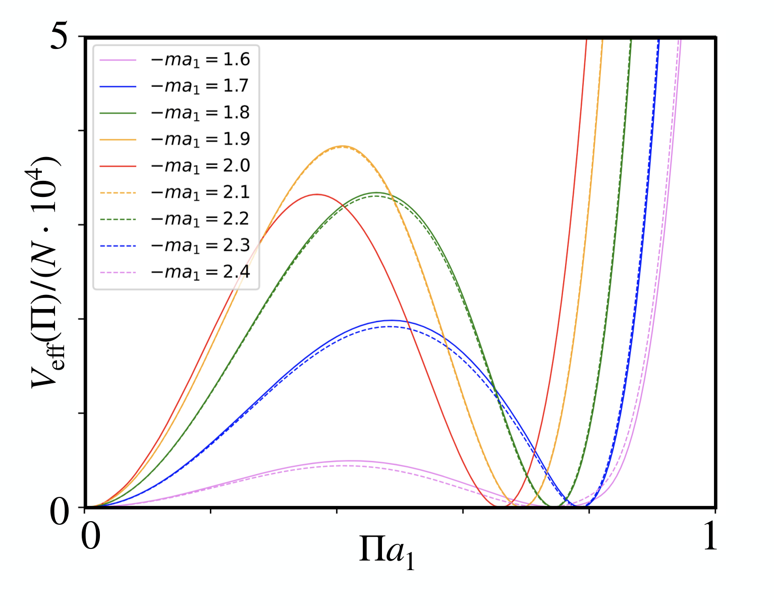
VI Spin-orbit-coupled Fermi gases
In the previous sections, we have presented a thorough study of the phase diagram of the four-Fermi-Wilson model (10), combining various tools developed by the condensed-matter, high-energy physics and quantum-information communities. We have seen that large- methods yield a powerful tool to identify how the QAH phases are modified by interactions, and to understand the nature of the topological and symmetry-breaking phase transitions. By focusing on the strong-coupling limit, we have also shown that the effective super-exchange interactions leading to a quantum compass model (31) can yield more accurate estimates of the position of the critical lines and, eventually, the corresponding scaling of the underlying strongly-coupled fixed point. This follows from our comparison of the large- predictions with two different variational methods for the compass model, which shows a clear deviation of the critical lines using the more-accurate iPEPS algorithm. Thus, it would be interesting if future work could apply this method to the full fermionic model, rather than the effective compass model, in order to explore arbitrary couplings. Another promising approach in this direction would be to use the discrete-time formulation based on Euclidean LFT (79)-(81) with dimensionless fields (82), in combination with Monte Carlo sampling techniques. In this way, one may evaluate thermodynamic observables based on the partition function of the model (57) beyond the large- limit. In this section, we discuss yet another alternative, that of quantum simulations (QSs) Feynman 1982; Cirac and Zoller 2012, where one exploits quantum-mechanical hardware to simulate a specific quantum many-body problem. We emphasise that these QSs have the potential of overcoming some of the limitations of the above alternatives to large- methods, as they could probe real-time dynamics regardless of entanglement growth, and would not be limited by any sign problem as one explores finite fermion densities.
In this section, we focus on QSs based on ultracold atoms in optical lattices Bloch et al. 2008. We present a detailed scheme for the QS of the four-Fermi-Wilson model using the so-called Raman optical lattices Liu et al. 2014a; Liu et al. 2014b; Wu et al. 2016; Sun et al. 2018; Song et al. 2018; Liang et al. 2021. These quantum simulators can be considered as Fermi gases with a specific synthetic spin-orbit coupling Galitski and Spielman 2013; Zhai 2015; Zhang and Liu, mimicking the coupling of the intrinsic angular momentum of the electron with its own motion Thomas 1926 in the solid state Bychkov and Rashba 1984; Dresselhaus 1955. Spin-orbit coupling has turned out to be a source of important recent developments in condensed matter, as it underlies the experimental discovery König et al. 2007; Hsieh et al. 2008 of a new mechanism for the ordering of matter Kane and Mele 2005a; Kane and Mele 2005b; Bernevig et al. 2006 in topological insulators and superconductors Hasan and Kane 2010; Qi and Zhang 2011; Chiu et al. 2016. Given the special role of Chern insulators and the QAH effect within these topological phases, it does not come as a surprise that spin-orbit coupling is somehow disguised in our four-Fermi-Wilson model (10). Additionally, given that the spin-orbit coupling is directly accounted for by the Dirac equation Dirac 1928; Dirac 1930 and, ultimately, by quantum electrodynamics Schweber 1994, it is natural that our discretization of a QFT of self-interacting Dirac fermions is also connected to spin-orbit coupling. Let us now discuss this connection in detail for our representation of the Clifford algebra (2).
Note that in spacetime dimensions, one can define rotations of angle around the normal vector of the spatial plane, which are generated by
| (114) |
For our particular choice of gamma matrices (2), the spinor representation of this rotation, which belongs to the Lorentz group , is generated by , such that the fields transform as
| (115) |
As noted in Sec. IV.1, the rotation leads, up to an irrelevant phase, to the inversion symmetry defined in Eq (61). Since this transformation can be generated infinitesimally, it does not correspond to parity symmetry.
In light of Eq. (115), the two spinor components for each flavour in the original QFT (1) can be identified with the spin up/down states of the fermions, respectively. From this perspective, the tunnellings of the naive discretization of the Hamiltonian field theory in Eq. (6), namely , are understood as the finite-difference discretization of the so-called Rashba spin-orbit coupling Bychkov and Rashba 1984, when written in terms of fermionic creation/annihilation operators in second quantization. From this perspective, the complete Wilson-type discretization in Eq. (10) can be considered as a Dirac-type spin-orbit coupling that generalises the aforementioned Rashba terms Zhang and Liu.
Once the connection to spin-orbit coupling has been clarified, we can exploit the ideas underlying the cold-atom QSs of synthetic spin-orbit coupling in optical lattices and, in particular, we discuss how the schemes in Liu et al. 2014a; Liu et al. 2014b can be adapted with minor modifications to realise our four-Fermi-Wilson model (10), as briefly discussed in Ziegler et al. 2020. We also note that the recent experimental realization of the Qi-Wu-Zhang model using Raman optical lattices Liang et al. 2021 is related to the non-interacting limit of our four-Fermi-Wilson model (10).
VI.1 Raman optical lattices and spin-flip tunnellings

Let us consider a gas of fermionic atoms, such as the alkali-earth 87Sr gas, which are subjected to interfering laser beams that generate a cubic optical potential Grimm et al. 2000, namely
| (116) |
Here, now labels all three spatial axes, is the wave-vector of the laser beams with mutually-orthogonal polarizations (see the blue and green arrows in Fig. 20(a)), which interfere along the -axis and lead to a standing-wave pattern. We have also introduced as the amplitude of the corresponding ac-Stark shift experienced by the atoms in the groundstate manifold , where is the total angular momentum, and are the possible Zeeman sub-levels split by an additional external magnetic field (we chose as the quantization axis in Fig. 20(a)). In this work, it suffices to focus on two such hyperfine levels in order to define the spinor components , choosing in a way that the electric-dipole selection rules allow one to connect these levels via two-photon Raman transitions. These two states can be isolated from the remaining hyperfine levels in the groundstate manifold by exploiting a Zeeman shift, or an ac-Stark shift as in the case of the 87Sr gas Liang et al. 2021, which must depend non-linearly on the magnetic number .
In order to induce the Raman transitions, one needs to drive off-resonant couplings to states within the excited-state manifold , which requires using large detunings to minimise spontaneous photon emission and the associated heating mechanisms, as depicted in the insets of Figs. 20 (b) and (c). These drivings can be obtained by two additional laser beams in a travelling-wave configuration, selecting their wave-vectors and polarizations (see the orange and red arrows in Fig. 20 (a)), following the general ideas of the schemes of synthetic spin-orbit coupling to create a Raman potential Zhang and Liu; Liu et al. 2014a; Liu et al. 2014b. We note that a standing-wave pattern for these Raman beams can also be used which, in analogy to the optical-lattice potential (116), can be obtained by exploiting retro-reflecting mirrors Wang et al. 2018, and underlies the recent implementation of synthetic spin-orbit coupling with the 87Sr gas Liang et al. 2021. We would also like to remark that there have been other realizations of synthetic spin-orbit coupling that do not rely on Raman lattice potentials, using alkaline-earth Kolkowitz et al. 2017; Bromley et al. 2018 and lanthanide Burdick et al. 2016; Song et al. 2016; Livi et al. 2016 atoms. In comparison to the alkalis, these atomic systems have ultra-narrow optical transitions and a larger fine-structure splitting of the excited states, which can be exploited for the QS of synthetic spin-orbit coupling minimizing the heating caused by the residual spontaneous emission from the excited-state manifold Cui et al. 2013; Wall et al. 2016, as originally discussed in the context of synthetic gauge fields Gerbier and Dalibard 2010; Goldman et al. 2014. As discussed in the following paragraphs, these nice features can also be exploited for the generation of Raman lattice potentials.
Let us start by focusing on the Raman transition along the axis (see Fig. 20 (b)). This transition is implemented by the standing-wave beams along the direction, and an additional Raman beam with wave-vector , polarization and relative phase , which propagates in a travelling-wave configuration along the axis (see Fig. 20 (a)). As depicted in the inset of Fig. 20 (b), since the standing wave is linearly polarised along the quantization direction, it can couple one of the groundstate spinors to an excited state with the same magnetic number. On the other hand, since the Raman beam is linearly polarised along a different direction, which corresponds to a linear combination of the two circular polarizations, it can impart the required angular momentum onto the atoms to connect this excited state to a groundstate spinor component of a different magnetic number through a dipole-allowed transition, i.e. . For the Raman transition along the axis, the description is analogous (see Fig. 20 (c)), but it is now the standing wave which can impart momentum into the atoms, whereas the Raman beam propagating along has linear polarization along the quantization axis. As discussed in more detail below, it is important to control the phase of this second Raman process relative to .
As depicted in the insets of Figs. 20 (b) and (c), when the detunings with respect to the excited states are very large, the two-photon processes only involve the spinor levels. Due to the participation of the standing wave, the Raman transition has a periodic intensity depicted with a green solid line in Figs. 20 (b)-(c), which has a doubled period with respect to the optical-lattice potentials depicted with blue solid lines (116). Altogether, the groundstate spinors are subjected to the Raman potential
| (117) |
where we have introduced , () is the Rabi frequency (detuning) of the Raman transition driven by the -th travelling wave, and we work in the interaction picture with respect to the atomic transition, such that are the detunings of the laser beatnotes with respect to the transition frequency (see the insets of Figs. 20 (b)-(c)). Let us note that, in principle, there can also be two-photon contributions from the standing- and travelling-wave beams that propagate along the same axis, but these will be highly off-resonant and contribute with higher-order shifts of the energy levels, which can be taken into account by adjusting the laser frequencies.
The gas of neutral atoms of mass subjected to the total potential is described in second quantization, as customarily Lewenstein et al. 2007; Bloch et al. 2008, and leads to the following non-relativistic Hamiltonian field theory
| (118) |
where are the creation/annihilation fields of fermionic atoms at position in the internal state , and we have introduced the so-called -wave scattering length , which determines the strength of the contact two-body collisions for these dilute and ultra-cold atomic gases.
We consider that all the laser beams have the same wavelength , such that they can actually be generated from a single laser source, using acusto-optical modulators to control the detunings . To obtain a lattice field theory, we make use of the Wannier basis Kohn 1959 in
| (119) |
As depicted in Figs. 20 (b)-(c), the Wannier functions are localised around the minima of the blue-detuned ac-Stark shift (116), namely
| (120) |
where . In Eq. (119), are dimensionless creation-annihilation operators of fermions in the lowest band of the optical lattice. As realised in the seminal works Jaksch et al. 1998; Greiner et al. 2002, in the regime of deep optical lattices, where the potential barriers are much larger than the recoil energy , the atoms are tightly confined within the minima, and the Hamiltonian field theory (118) can be expressed in terms of a lattice model with nearest-neighbor couplings. For instance, the kinetic, ac-Stark shift and interaction potentials lead to a spin-conserving tunnelling and density-density interactions
| (121) |
where the fermion number operators are . Here, the tunnelling amplitudes
| (122) |
and interaction strengths
| (123) |
are obtained by overlap integrals of the Wannier functions, weighted by the kinetic and ac-Stark potentials or the interaction potential, respectively Bloch et al. 2008. Note that these overlaps can in principle couple neighbouring sites that lie further apart, but the corresponding strengths decay exponentially fast with distance Jaksch et al. 1998, and are thus routinely neglected. By increasing the standing-wave intensity along the -axis, such that , the dynamics of the atoms along the direction is effectively frozen, and Eq. (121) corresponds to the 2D Fermi-Hubbard model Hubbard 1963; Hofstetter et al. 2002 which, as discussed in the introduction, is a paradigm in the physics of strongly-correlated materials Imada et al. 1998; Lee et al. 2006. This Hamiltonian will be supplemented by additional tunnelling terms stemming from the Raman potential (117), which we now discuss in detail.
A crucial ingredient of the QSs of synthetic spin-orbit coupling using Raman potentials Zhang and Liu is that, due to the specific form of the light interference in Eq. (117), the corresponding overlaps of Wannier functions cannot contribute with local Raman transitions whereby an atom remains tightly trapped in a minimum of the optical potential, while its spin gets flipped . In the scheme of Figs. 20 (b)-(c), the vanishing of these on-site spin flips could be easily understood in the limit of weak Raman potentials , as a consequence of the zero value of this potential at the minima of the optical lattice (120). Remarkably, due to our choice of equal laser wave-vectors, symmetry arguments allow to prove that this is not limited to weak potentials. Mathematically, whereas the Wannier functions localised with respect to a single site are even with respect to lattice inversion about the site center (120) (see the schematic drawing in Figs. 20 (b)-(c)), the Raman potential (117) is odd, such that the corresponding overlap integrals vanish. The situation changes for the overlap between nearest-neighbour Wannier functions, as the above symmetry argument no longer applies in the direction of tunnelling. These overlaps lead to a non-zero spin-flip tunneling with a complex-valued amplitude
| (124) |
The modulus of the tunnelling, , can be estimated analytically by approximating the optical-lattice potential around the minima (120) by a harmonic oscillator of frequencies along each axis, such that the Wannier functions become a separable product of Gaussians. When tunnelling along the axis, the above symmetry argument can still be applied to neglect the () contribution of the Raman potential (117) to the overlap integral along the () axis. On the other hand, the () part gives a non-zero contribution multiplying the overlaps along the () axis, and leads to
| (125) |
In addition, one obtains a site-dependent phase
| (126) |
In the schemes of Figs. 20 (b)-(c)), the alternation of the signs of the spin-flip tunnellings can be understood as a consequence of the doubled period of the Raman potential with respect to the optical lattice, which leads to alternating signs of the linear slopes of the Raman potential as one moves along the tunnelling direction. As discussed in the following subsection, this is another crucial property for the QS of our four-Fermi-Wilson model.
VI.2 Four-Fermi-Wilson quantum simulator
Once we have obtained the microscopic Hamiltonian governing the dynamics of the two-component atoms in a deep optical Raman potential, we can discuss how this can be mapped via a gauge transformation, followed by a rescaling, to the four-Fermi-Wilson model of Eq. (10) in the single-flavour limit . This transformation is
| (127) |
The time-dependence can be understood as a change from the aforementioned interaction picture to the so-called rotating frame, such that the detunings correspond to an energy imbalance that will contribute to the bare mass. In addition, the site-dependent phase transformation allows us to rewrite the model in a translationally-invariant manner, making direct connection with the starting point for the lattice discretization of our four-Fermi-Wilson QFT discussed in Sec. II.2.
As discussed in Ziegler et al. 2020, the dependence on the relative phases generalises previous schemes for synthetic spin-orbit coupling Liu et al. 2014a; Liu et al. 2014b, which can be exploited to connect precisely to our four-Fermi-Wilson models. Setting the Raman-beam phases to , we find that the sum of the spin-conserving (121) and spin-flipping (124) Hamiltonians maps directly to the lattice field theory (10) with the following correspondence of the microscopic parameters
| (128) |
Accordingly, the bare mass can be controlled by the detuning of the Raman beams, whereas the coupling strength is proportional to the -wave scattering length (123), and can thus be modified independently via a Feshbach resonance Chin et al. 2010. Alternatively, since it is inversely proportional to the spin-flip tunnellings (125), one can tune this parameter by modifying the corresponding potential depths or . At this point, it is worth mentioning that the recent experimental realization of the Qi-Wu-Zhang model with the 87Sr gas Liang et al. 2021 is related to the non-interacting limit of our four-Fermi-Wilson model (10) by a simple rotation of gamma matrices (2) that makes . In this case, the experiment uses standing-wave Raman beams, and their relative phase enters differently in the microscopic Hamiltonian. The only important point is that this phase difference is . In the presence of the Hubbard interactions, this would only lead to an interchange of the two symmetry-breaking channels. We thus believe that these experiments are a very promising route to explore the physics discussed in our work.
In this regard, it is important to note that the effective lattice spacings are not set by the optical-lattice wavelength , but rather by the inverse of the spin-flip tunnelling strengths, which are proportional to the Rabi frequency of the Raman beams (125), and can thus be tuned by changing the corresponding laser power. Since this laser power can be different along the axes, the cold-atom QS can also explore different anisotropies for the spatial , and Wilson parameters . In this manuscript, we have explored in detail the limit , which would require equal spin-conserving and spin-flip tunnellings. We note, however, that non-unity Wilson parameters will simply rescale the axes but maintain the same shape of the non-interacting phase diagram. As the interactions are switched on, we expect that will not introduce additional strong-coupling phases. Exploring larger or smaller values is left for future studies, which could also be targeted by the proposed QS.
Let us now comment on the observable consequences of the gauge transformation (127). The time-dependence due to the rotating frame is customary in quantum optics, and can be accounted for during the measurement process. The local site-dependent phase can change the interpretation of the symmetry-breaking order parameters related to the -field condensates, while they do not change the -field scalar condensate. One can easily check that
| (129) |
Accordingly, in the language of the cold-atom QS, a non-zero value of the scalar condensate corresponds to an atomic density imbalance between the two hyperfine groundstates. For the Lorentz-breaking condensates the situation changes, as a non-zero value marks an alternating pattern that turns the orbital ferromagnets FMx (FMy) into Néel-ordered anti-ferromagnets AFMx (AFMy). In order to prepare these phases, as well as the correlated QAH or trivial band insulators discussed in this manuscript, one would start by preparing an ultra-cold spin-polarised Fermi gas by optical pumping, and then adiabatically ramping up the ac-Stark and Raman potentials to create the non-interacting groundsate for specific values of . One could then adiabatically change the coupling strength . According to Eq. (128), one can increase the Hubbard interactions via a Feshbach resonance, or decrease the spin-flip tunnellings, until the desired point of parameter space is reached. Once this groundstate is approximately prepared, let us discuss possible characterization techniques in the experiment.
Note that the scalar condensate (129) can be inferred by spin-resolved in-situ imaging, where the trapped atoms are illuminated by an incoming laser and cast a shadow on a CCD-camera that is used to extract the integrated, so-called columnar, density of the atoms Ketterle et al. 1999; Ketterle and Zwierlein 2008. Absorptive Partridge et al. 2006 and dispersive Shin et al. 2006 techniques can be applied in subsequent shots with lasers addressing each of the internal states separately, such that can be reconstructed from the spin-resolved columnar densities. To get lattice-site resolution for , one can exploit the so-called quantum gas microscopes Kuhr 2016; Bakr et al. 2009; Sherson et al. 2010; Haller et al. 2015; Cheuk et al. 2016a; Greif et al. 2016. To achieve spin resolution, one may separate different spin components spatially prior to the microscope imaging Weitenberg et al. 2011; Boll et al. 2016. Alternatively, one can remove the atoms with a specific spin state by shining resonant light before the imaging Parsons et al. 2016; Cheuk et al. 2016b. Finally, in order to infer the values of the condensates, one would need to apply an additional microwave/Raman term that drives a rotation of the spins on the Bloch sphere in Fig. 5 (a). Controlling the phase of this rotation, provided that it is locked to the rotating frame of the original Raman beams, one can map the differential spin population to the or axis, such that the subsequent quantum-gas-microscope imaging gives the desired information about the Lorentz-breaking condensates (129).
Density imaging can also be performed after switching off the confining potential, which leads to the so-called time-of-flight (TOF) imaging. If the density is imaged after a sudden release Greiner et al. 2002, one gains information about the coherence properties of the system in momentum space Bloch et al. 2008. Instead of the sudden release, one can adiabatically ramp-down the lattice potential, which gives access to the quasi-momentum atomic distribution through the so-called band-mapping technique Greiner et al. 2001; Köhl et al. 2005. In reference Jotzu et al. 2014, this band-mapping technique was used to measure the differential drift of the atom cloud when subjected to two opposite gradients, which allows one to distinguish trivial from non-trivial Berry curvatures in Haldane’s honeycomb model of the QAH effect. This type of measurements could be used to infer the value of the Chern number Price and Cooper 2012; Dauphin and Goldman 2013, as has been demonstrated in cold-atom experiments of the integer QHE Aidelsburger et al. 2014.
Coming back to the QAH effect, we note that the spin-resolved TOF densities have been measured in quasi-momentum space for the simulated Qi-Wu-Zhang model with the 87Sr gas Liang et al. 2021. Remarkably, exploiting a symmetry that corresponds exactly to our inversion symmetry (61), the measured differential spin densities at four high-symmetry points of the Brillouin zone give experimental access to the Chern number Liu et al. 2013. These points correspond to the center , edge centers and corner where the fermion doublers reside, as discussed below Eq. (17). According to our discussion of the static self-energy and the topological Hamiltonian in Sec. V.2, we expect that these spin densities will get renormalized by the non-zero scalar condensate, but still serve to characterise the topological invariant in the presence of interactions in an analogous fashion to our Eq. (112). It would be interesting to combine this observable, together with the in-situ symmetry-breaking () condensates, to explore the full phase diagram of the model and the topological and symmetry-breaking phase transitions. We note that, in this case, the condensates would change into AFMy (AFMx) Néel orders due to the alternation in Eq. (129), and the change of the different implementation of the Raman lattice.
Before closing this section, we emphasise that recovering the continuum limit of the lattice field theory (10) implemented by the cold-atom QS does not imply a drastic modification of the laser wavelength . Instead, it requires setting the microscopic parameters to certain values, such that the bare couplings lie in the vicinity of a critical point. Here, the energy gap is much smaller than the tunnellings , and the relevant length scale leads to a continuum QFT. The question that could be addressed by the cold-atom QS is to explore this region and determine the critical scaling shedding light on the nature of the strongly-coupled fixed points of the continuum four-Fermi QFT, addressing questions that might otherwise require large-scale LFT simulations. Ultimately, the goal would be to explore different fillings and real-time dynamics in these models, going beyond the capabilities of classical simulations.
VII Conclusion and outlook
We have shown that Wilson-type discretizations of four-Fermi QFTs in (2+1) dimensions (1) with irreducible representations of the gamma matrices (2) yield a neat playground to address interesting questions in both high-energy physics and condensed matter. Although explicitly lacking chiral symmetry, these regularised QFTs present the analogue of dynamical mass generation which, in contrast to other spacetime dimensions, occurs both at a non-zero coupling strength within a renormalizable QFT with a strongly-coupled fixed point. In contrast to chiral-invariant theories, these four-Fermi-Wilson model can also host fermion condensates that break inversion symmetry spontaneously and, thus, Lorentz invariance in the continuum limit. From a condensed-matter perspective, these lattice models host QAH phases with non-zero Chern numbers, and the four-Fermi terms can be used to explore the role of interactions as one enters strongly-correlated regimes. Both of these topics are actively investigated in these two fields.
We have presented a multidisciplinary approach that combines tools from these communities to advance our understanding of these four-Fermi-Wilson models. In the strong-coupling and single-flavour limit, we have shown that the condensed-matter concept of super-exchange interactions can be used to find an effective description in terms of a 900 quantum compass model in a transverse field. Analyzing this model with variational mean-field and tensor-network techniques, we have identified two possible symmetry-breaking channels that connect to two versions of the aforementioned Lorentz-breaking condensates. This has allowed us to formulate a large- limit of this field theory in terms of auxiliary fields, which has been used to predict the whole extent of the condensates away from the strong-coupling limit by solving a set of non-linear gap equations. By comparing a continuum-time Hamiltonian formalism with a discrete-time Euclidean approach, we have been able to identify additive renormalizations of the bare parameters that must be carefully considered when one explores the phases of the model using the discrete-time Euclidean approach common to the lattice field theory community.
Moreover, using the Euclidean approach, we have calculated the effective potential resumming the leading-order Feynman diagrams for . This has allowed us to unveil a new type of radiative corrections that give rise to novel effects in comparison to chiral-invariant theories, such as an interesting crossover between first- and second-order phase transitions. This effective potential has also allowed us to explore regions of parameter space where the inversion symmetry remains intact, extracting the large- contributions to the self-energy, and using those to calculate the many-body Chern numbers that characterise the groundstate and the QAH in the presence of correlations. This leads to a non-perturbative characterization of a rich phase diagram, which contains large- Chern insulators, trivial band insulators, and Lorentz-breaking fermion condensates separated by various critical lines, around which one can recover continuum QFTs and explore the nature of the corresponding strongly-coupled fixed points.
Finally, we have shown that quantum simulators based on ultra-cold alkali-earth atoms trapped in optical lattices and subjected to synthetic spin-orbit coupling yield a very promising avenue to realise these four-Fermi-Wilson models in experiments. In particular, we have argued that recent experiments with a 87Sr gas subjected to Raman lattice potentials Liang et al. 2021 is related to the non-interacting limit of our four-Fermi-Wilson model, and gives a unique opportunity to explore a correlated QAH effect in the laboratory. Such an implementation would benefit from the microscopic tunability of cold-atom quantum gases, which would allow to infer all of the relevant observables such as the symmetry-breaking order parameters related to the fermion condensates or the many-body Chern numbers. Moreover, these quantum simulators would open the route to the study of real-time dynamics and finite-fermion densities, overcoming current limitations of numerical studies based on classical hardware.
As an outlook, we believe that exploiting the current multi-disciplinary view will be very interesting to explore effects that have not been covered by this article. An interesting open question is to determine the role of anisotropic Wilson parameters in the nature of the Lorentz-breaking fermion condensates, exploring if new phases can appear as one increases the interactions. We also believe that further studies of the isotropic regime will be very interesting. As noted in this manuscript, there is an emerging symmetry in the field, which can modify substantially the dynamics of the theory due to an additional Chern-Simons term that is generated by quantum corrections. In analogy to quantum electrodynamics in (2+1) dimensions, where photons acquire a mass due to a Chern-Simons term Redlich 1984b, the low-lying excitations about the condensate phase that breaks the symmetry spontaneously can also acquire a non-zero mass. It will be very interesting to explore this phenomenon in the presence of boundaries, since there can be an interplay with the QAH effect and the topological edge states. Finally, we finish by mentioning that the cold-atom quantum simulators would open a new route to the study of real-time dynamics and finite-fermion densities, overcoming current limitations of numerical studies based on classical hardware. In the future, it will be very interesting to exploit this multidisciplinary view and to identify new interaction-induced topological phases, such as fractional Chern insulators.
Acknowledgements
The ICFO group acknowledges support from ERC AdG NOQIA, State Research Agency AEI (“Severo Ochoa” Center of Excellence CEX2019-000910-S) Plan National FIDEUA PID2019-106901GB-I00 project funded by MCIN/ AEI /10.13039/501100011033, FPI, QUANTERA MAQS PCI2019-111828-2 project funded by MCIN/AEI /10.13039/501100011033, Proyectos de I+D+I “Retos Colaboración” RTC2019-007196-7 project funded by MCIN/AEI /10.13039/501100011033, Fundació Privada Cellex, Fundació Mir-Puig, Generalitat de Catalunya (AGAUR Grant No. 2017 SGR 1341, CERCA program, QuantumCAT U16-011424, co-funded by ERDF Operational Program of Catalonia 2014-2020), EU Horizon 2020 FET-OPEN OPTOLogic (Grant No 899794), and the National Science Centre, Poland (Symfonia Grant No. 2016/20/W/ST4/00314), Marie Skłodowska-Curie grant STREDCH No 101029393, “La Caixa” Junior Leaders fellowships (ID100010434), and EU Horizon 2020 under Marie Skłodowska-Curie grant agreement No 847648 (LCF/BQ/PI19/11690013, LCF/BQ/PI20/11760031, LCF/BQ/PR20/11770012).). A.B. acknowledges support from the Ramón y Cajal program RYC-2016-20066, CAM/FEDER Project S2018/TCS- 4342 (QUITEMADCM), and PGC2018-099169-B-I00 (MCIU/AEI/FEDER, UE). S.J.H. acknowledges the support of STFC grant ST/T000813/1.
Appendix A Absence of two simultaneous condensates
In this Appendix, we give a detailed account of the gap equations obtained by using a Hubbard-Stratonovich transformation to rewrite the action (58) in terms of two fields, and show that there cannot be a simultaneous condensation for general anisotropies.
To find the effective action in terms of the and auxiliary fields, we note that in the single-flavour limit one can exactly rewrite the quartic interaction as the combination , such that the auxiliary fields can be introduced symmetrically. We proceed by assuming once more that the corresponding condensates are homogeneous, i.e. , , such that the effective action is now
| (130) |
Here, in analogy to the derivation for a single channel presented in Sec. IV.1, we find that the single-particle Hamiltonian (13) gets modified to
| (131) |
where the vector (14) also gets modified due to the presence of the auxiliary fields
| (132) |
Therefore, the only differences with respect to Sec. IV.1 are that the couplings strength , and that this vector is simultaneously shifted by both condensates.
The rest of the derivation follows exactly the steps described in Sec. IV.1, and leads to a saddle point of the action that is now determined by three non-linear gap equations
| (133) | ||||
| (134) | ||||
| (135) |
Let us note that from II (134) and III (135), it follows that
| (136) |
The left hand side does not vanish for any point (, , ) in the anisotropic case , meaning that II and III cannot be satisfied simultaneously. For , gap equations II and III are equal and, around this regime, Eq. (136) changes from being negative to positive. As a consequence, there is no condensation with two simultaneous non-zero vacuum expectation values of the fields for generic anisotropy, meaning that we must consider either the or the symmetry-breaking channels individually. This is in line with the prediction of the variational mean-field where, in the language of an effective spin model, the ground state is either a - or -ferromagnet unless . This discussion implies that we can improve on the auxiliary-field description by considering two independent sets of gap equations for and separately.
Appendix B Continuum-time limit and time doublers
In this Appendix, we present a detailed derivation of the additive renormalization of the bare parameters in the time-continuum limit (98) caused by the spurious time doublers (95). To get an explicit expression for this renormalization, we start from the action for dimensional fields (78), using a subscript in the bare parameters and condensates to distinguish this discrete-time Euclidean-lattice approach from the Hamiltonian one in Eqs. (70)-(71).
After repeating similar steps as those described in Sec. IV.1, we obtain an effective action for the auxiliary fields, and arrive at a pair of gap equations
| (137) | ||||
| (138) |
where the Euclidean contribution to the mass (92) due to the Wilson-term reads, for dimensional couplings, as follows
| (139) |
In the above gap equations, we have also introduced the analogue of Eq. (91) for dimensional couplings
| (140) |
With these expressions at hand, let us perform a long-wavelength approximation around , such that we can identify the contributions of the physical and spurious doublers. After a Taylor expansion, and using contour techniques for the integrals along , we find that the second gap equation can be expressed as
| (141) |
where , and we have made use of the single-particle energy defined in Eq. (68). We can now let , noticing that the mass term of the spurious time doublers, proportional to , dominates in the denominator of the second term, such that the integral vanishes linearly with in this limit. Accordingly, we recover the continuum gap equation (71) for , which is the desired single -channel gap equation. Let us now recall that, in our numerical solution of the gap equations, we start by fixing the value of the coupling strength and , after which we solve Eq. (138) to get the condensate . As we have just shown that the Euclidean-lattice gap equation (138) yields the same gap equation (71) in the continuum-time limit, we can thus conclude that
| (142) |
The situation changes for the first gap equation (137), since the Wilson-term contribution (139) for the time doublers leads to a term that scales with also in the numerator
| (143) | ||||
In the limit , the second term no longer vanishes, but yields instead
| (144) |
One can readily check that this gap equation differs from the Hamiltonian one (70), which was obtained by working directly in the time-continuum limit, by a constant additive term, where we consider the single -channel. Going back to our numerical solution of the gap equations, and the discussion above Eq. (142), once we have solved the second gap equation and know and , we can solve Eq. (138) to obtain the value of the scalar condensate , and finally infer the corresponding bare mass . According to the shift in equation (144), we can readily infer that the Euclidean-lattice formalism gives the same value of the scalar condensate, but renormalizes additively the bare mass
| (145) |
When this additive renormalization is taken into account, together with the required rescalings of the adimensional formulation (82), we finally arrive to Eq. (98).
Appendix C Derivation of the effective potential
In this Appendix, we give a detailed account of the derivation of the resummation for the effective potential (101) to all orders of the couplings strength . Let us start from the most general expression with an even/odd number of auxiliary lines
| (146) | ||||
where we recall that , with , and our choice for the Euclidean gamma matrices is given in Eq. (80). Although these are the specific for the anisotropic Wilson-type regularization of the four-Fermi QFT, we note that the following derivations are completely generic, and can be readily applied to the continuum case and to other representations of gamma matrices. For instance, if one aims at implementing chiral symmetry using the Euclidean version of Eq. (3), the expressions below need only be modified by letting due to the doubled dimension of the gammas.
The trace in Eq. (146) can be calculated analytically via an inductive method, where
| (147) |
and we have defined
| (148) |
One can derive a recursive relation by noting that
| (149) | ||||
| (150) |
In the last step, we use the anti-commutation rules , and the identity . The recurrence relation starts with the first two terms and which, considering our choice in Eq. (80) and the properties of the Pauli matrices, have the traces
| (151) |
For higher-dimensional representations, such as Eq. (3), these traces will have an overall multiplicative factor that shall carry onto the expressions of the effective potential.
With the aid of these first two terms, and the above recurrence relation, one can develop a general expression for arbitrary with the general structure
| (152) |
where the first few values of the coefficients are given in Table 1. Note that we only present the coefficients for even integers , and even . Although the odd ones , for odd , can also be non-zero, they lead to mode sums, or integrals in the continuum, which vanish (146), as the function is odd in a symmetric interval. In the standard calculation of the effective potential for continuum four-Fermi QFTs Coleman 1985, where the field couples to for the chiral symmetry-breaking channel; the odd terms vanish directly since they are proportional to the traces of the gamma matrices, all of which vanish. For the current channel, although the traces do not vanish, once we integrate over the Euclidean Brillouin zone (146), the odd terms do not contribute either. It is for this reason that the large- Feynman diagrams depicted in Fig. only contain an even number of auxiliary lines, and lead to Eq. (146).
| 0 | 2 | 4 | 6 | 8 | 10 | 12 | |
| 2 | 2 | ||||||
| 4 | 1 | 8 | |||||
| 6 | 18 | 32 | |||||
| 8 | 1 | 160 | 128 | ||||
| 10 | 512 | ||||||
| 12 | 2048 | ||||||
In order to perform the resummation, we need to express these coefficients in closed from. We have found that the exact expression is
| (153) |
where we have introduced
| (154) |
The first values of shown in table 1 can be readily checked to follow this general expression. This expression (153) must be supplemented with the term . Relabelling to only account for terms with an even number of external lines, we find
| (155) |
where the first radiative term comes from resumming the series in for the aforementioned term, where we have used for the parameter
| (156) |
such that convergence requires . We note that in the standard effective potential for continuum four-Fermi QFTs Coleman 1985, where the field couples to the bilinear, all the radiative quantum corrections to the classical potential are contained in a term that is completely analogous to this one
| (157) |
after making the substitution . Accordingly, the consequence of using a different channel is that there are additional quantum corrections contained in the remaining contributions for of Eq. (155). Accounting for these new radiative corrections is crucial to find the correct phase diagram, identifying the regions that delimit the correlated QAH phase.
Let us now describe how to perform the resummation of these additional corrections. The idea is to focus on the different contributions separately, performing the sums over to arbitrary orders of the coupling strength, here corresponding to arbitrary pairs of external lines, by means of the following generating functions
Note that the contributions in Eq. (155) of order , considering a fixed value of , can be expressed in terms of a combination of generating functions , e.g. for one gets a contribution proportional to . Each of these generating functions is a rational function , the numerator of which is a polynomial of order . In light of Eq. (156), , and one would then expect that each term has a different polynomial dependence on the condensate, such that resummation cannot be performed. Remarkably, we find that the prefactors that multiply the generating functions inside each of the polynomials cancel all terms except for one scaling with , e.g. for , we get . This leads to a scaling with the condensate of order that can now be resummed. The first few terms of these additional quantum-mechanical corrections to the effective potential read
| (158) |
The particular form of these last four terms suggests that a resummation is possible using again the the Taylor series of the logarithm series, such that
References
- Sachdev (2011) S. Sachdev, Quantum Phase Transitions, 2nd ed. (Cambridge University Press, 2011).
- Landau (1937) L. Landau, Zh. Eksp. Teor. Fiz. 7, 19 [Phys. Z. Sowjetunion 11, 26 (1937)] (1937).
- Ginzburg and Landau (1950) V. Ginzburg and L. Landau, Zh. Eksp. Teor. Fiz. 20, 1064 (1950).
- Anderson (1972) P. W. Anderson, Science 177, 393 (1972).
- Altland and Simons (2006) A. Altland and B. Simons, “Frontmatter,” in Condensed Matter Field Theory (Cambridge University Press, 2006) pp. i–iv.
- Fazekas (1999) P. Fazekas, Lecture Notes on Electron Correlation and Magnetism (World Scientific, 1999).
- Hubbard (1963) J. Hubbard, Proc. R. Soc. London, Ser. A 276, 238 (1963).
- Imada et al. (1998) M. Imada, A. Fujimori, and Y. Tokura, Rev. Mod. Phys. 70, 1039 (1998).
- Anderson (1950) P. W. Anderson, Phys. Rev. 79, 350 (1950).
- Anderson (1963) P. W. Anderson (Academic Press, 1963) pp. 99 – 214.
- Anderson (1987) P. W. Anderson, Science 235, 1196 (1987).
- Lee et al. (2006) P. A. Lee, N. Nagaosa, and X.-G. Wen, Rev. Mod. Phys. 78, 17 (2006).
- Fermi (1934) E. Fermi, Zeitschrift für Physik 88, 161 (1934).
- Wilson (1968) F. L. Wilson, American Journal of Physics 36, 1150 (1968).
- Nambu and Jona-Lasinio (1961a) Y. Nambu and G. Jona-Lasinio, Phys. Rev. 122, 345 (1961a).
- Nambu and Jona-Lasinio (1961b) Y. Nambu and G. Jona-Lasinio, Phys. Rev. 124, 246 (1961b).
- Klevansky (1992) S. P. Klevansky, Rev. Mod. Phys. 64, 649 (1992).
- Gross and Neveu (1974) D. J. Gross and A. Neveu, Phys. Rev. D 10, 3235 (1974).
- Wilson (1974) K. G. Wilson, Phys. Rev. D 10, 2445 (1974).
- Gattringer and Lang (2010) C. Gattringer and C. B. Lang, Quantum chromodynamics on the lattice: an introductory presentation (Springer, 2010).
- Hands (1997) S. Hands, “Fixed point four-fermi theories,” (1997), arXiv:hep-lat/9706018 .
- Creutz (1997) M. Creutz, Quarks, gluons and lattices (Cambridge University Press, 1997).
- Castro Neto et al. (2009) A. H. Castro Neto, F. Guinea, N. M. R. Peres, K. S. Novoselov, and A. K. Geim, Rev. Mod. Phys. 81, 109 (2009).
- Armitage et al. (2018) N. P. Armitage, E. J. Mele, and A. Vishwanath, Rev. Mod. Phys. 90, 015001 (2018).
- Qi and Zhang (2011) X.-L. Qi and S.-C. Zhang, Rev. Mod. Phys. 83, 1057 (2011).
- Hasan and Kane (2010) M. Z. Hasan and C. L. Kane, Rev. Mod. Phys. 82, 3045 (2010).
- Schnyder et al. (2008) A. P. Schnyder, S. Ryu, A. Furusaki, and A. W. W. Ludwig, Phys. Rev. B 78, 195125 (2008).
- Kitaev (2009) A. Kitaev, AIP Conference Proceedings 1134, 22 (2009).
- Chiu et al. (2016) C.-K. Chiu, J. C. Y. Teo, A. P. Schnyder, and S. Ryu, Rev. Mod. Phys. 88, 035005 (2016).
- Soumyanarayanan et al. (2016) A. Soumyanarayanan, N. Reyren, A. Fert, and C. Panagopoulos, Nature 539, 509 (2016).
- Klitzing et al. (1980) K. v. Klitzing, G. Dorda, and M. Pepper, Phys. Rev. Lett. 45, 494 (1980).
- Thouless et al. (1982) D. J. Thouless, M. Kohmoto, M. P. Nightingale, and M. den Nijs, Phys. Rev. Lett. 49, 405 (1982).
- Nakahara (2017) M. Nakahara, Geometry, Topology and Physics (CRC Press, 2017).
- Niu et al. (1985) Q. Niu, D. J. Thouless, and Y.-S. Wu, Phys. Rev. B 31, 3372 (1985).
- Halperin (1982) B. I. Halperin, Phys. Rev. B 25, 2185 (1982).
- Hatsugai (1993) Y. Hatsugai, Phys. Rev. Lett. 71, 3697 (1993).
- Haldane (1988) F. D. M. Haldane, Phys. Rev. Lett. 61, 2015 (1988).
- Qi et al. (2006) X.-L. Qi, Y.-S. Wu, and S.-C. Zhang, Phys. Rev. B 74, 085308 (2006).
- Qi et al. (2008) X.-L. Qi, T. L. Hughes, and S.-C. Zhang, Phys. Rev. B 78, 195424 (2008).
- Liu et al. (2016) C.-X. Liu, S.-C. Zhang, and X.-L. Qi, Annual Review of Condensed Matter Physics 7, 301 (2016).
- Kane and Mele (2005a) C. L. Kane and E. J. Mele, Phys. Rev. Lett. 95, 146802 (2005a).
- Kane and Mele (2005b) C. L. Kane and E. J. Mele, Phys. Rev. Lett. 95, 226801 (2005b).
- Niemi and Semenoff (1983) A. J. Niemi and G. W. Semenoff, Phys. Rev. Lett. 51, 2077 (1983).
- Redlich (1984a) A. N. Redlich, Phys. Rev. Lett. 52, 18 (1984a).
- Redlich (1984b) A. N. Redlich, Phys. Rev. D 29, 2366 (1984b).
- Semenoff (1984) G. W. Semenoff, Phys. Rev. Lett. 53, 2449 (1984).
- Nielsen and Ninomiya (1981a) H. Nielsen and M. Ninomiya, Nuclear Physics B 185, 20 (1981a).
- Nielsen and Ninomiya (1981b) H. Nielsen and M. Ninomiya, Nuclear Physics B 193, 173 (1981b).
- Wilson (1977) K. G. Wilson, in New Phenomena in Subnuclear Physics (Springer US, 1977) pp. 69–142.
- Kogut and Susskind (1975) J. Kogut and L. Susskind, Phys. Rev. D 11, 395 (1975).
- Kaplan (1992) D. B. Kaplan, Physics Letters B 288, 342 (1992).
- So (1985) H. So, Progress of Theoretical Physics 73, 528 (1985).
- Golterman et al. (1993) M. F. Golterman, K. Jansen, and D. B. Kaplan, Physics Letters B 301, 219 (1993).
- Chang et al. (2013) C.-Z. Chang, J. Zhang, X. Feng, J. Shen, Z. Zhang, M. Guo, K. Li, Y. Ou, P. Wei, L.-L. Wang, Z.-Q. Ji, Y. Feng, S. Ji, X. Chen, J. Jia, X. Dai, Z. Fang, S.-C. Zhang, K. He, Y. Wang, L. Lu, X.-C. Ma, and Q.-K. Xue, Science 340, 167 (2013).
- Chang et al. (2015) C.-Z. Chang, W. Zhao, D. Y. Kim, H. Zhang, B. A. Assaf, D. Heiman, S.-C. Zhang, C. Liu, M. H. W. Chan, and J. S. Moodera, Nature Materials 14, 473 (2015).
- Yu et al. (2010) R. Yu, W. Zhang, H.-J. Zhang, S.-C. Zhang, X. Dai, and Z. Fang, Science 329, 61 (2010).
- Deng et al. (2020) Y. Deng, Y. Yu, M. Z. Shi, Z. Guo, Z. Xu, J. Wang, X. H. Chen, and Y. Zhang, Science 367, 895 (2020).
- Zhao et al. (2020) Y.-F. Zhao, R. Zhang, R. Mei, L.-J. Zhou, H. Yi, Y.-Q. Zhang, J. Yu, R. Xiao, K. Wang, N. Samarth, M. H. W. Chan, C.-X. Liu, and C.-Z. Chang, Nature 588, 419 (2020).
- Zhao et al. (2021) Y.-F. Zhao, R. Zhang, L.-J. Zhou, R. Mei, Z.-J. Yan, M. H. W. Chan, C.-X. Liu, and C.-Z. Chang, “Zero magnetic field plateau phase transition in higher chern number quantum anomalous hall insulators,” (2021), arXiv:2109.11382 .
- Hohenadler and Assaad (2013) M. Hohenadler and F. F. Assaad, Journal of Physics: Condensed Matter 25, 143201 (2013).
- Bergholtz and Liu (2013) E. J. Bergholtz and Z. Liu, International Journal of Modern Physics B 27, 1330017 (2013).
- Neupert et al. (2015) T. Neupert, C. Chamon, T. Iadecola, L. H. Santos, and C. Mudry, Physica Scripta T164, 014005 (2015).
- Rachel (2018) S. Rachel, Reports on Progress in Physics 81, 116501 (2018).
- Hatsugai (2006) Y. Hatsugai, Journal of the Physical Society of Japan 75, 123601 (2006).
- Kudo et al. (2019) K. Kudo, H. Watanabe, T. Kariyado, and Y. Hatsugai, Phys. Rev. Lett. 122, 146601 (2019).
- Wang et al. (2010) Z. Wang, X.-L. Qi, and S.-C. Zhang, Phys. Rev. Lett. 105, 256803 (2010).
- Gurarie (2011) V. Gurarie, Phys. Rev. B 83, 085426 (2011).
- Wang and Zhang (2012a) Z. Wang and S.-C. Zhang, Phys. Rev. X 2, 031008 (2012a).
- Wang and Zhang (2012b) Z. Wang and S.-C. Zhang, Phys. Rev. B 86, 165116 (2012b).
- Wang and Yan (2013) Z. Wang and B. Yan, Journal of Physics: Condensed Matter 25, 155601 (2013).
- Li and Haldane (2008) H. Li and F. D. M. Haldane, Phys. Rev. Lett. 101, 010504 (2008).
- Pollmann et al. (2010) F. Pollmann, A. M. Turner, E. Berg, and M. Oshikawa, Phys. Rev. B 81, 064439 (2010).
- Zaletel et al. (2014) M. P. Zaletel, R. S. K. Mong, and F. Pollmann, Journal of Statistical Mechanics: Theory and Experiment 2014, P10007 (2014).
- Budich et al. (2012) J. C. Budich, R. Thomale, G. Li, M. Laubach, and S.-C. Zhang, Phys. Rev. B 86, 201407 (2012).
- Wang et al. (2012) L. Wang, H. Jiang, X. Dai, and X. C. Xie, Phys. Rev. B 85, 235135 (2012).
- Raghu et al. (2008) S. Raghu, X.-L. Qi, C. Honerkamp, and S.-C. Zhang, Phys. Rev. Lett. 100, 156401 (2008).
- Sun et al. (2009) K. Sun, H. Yao, E. Fradkin, and S. A. Kivelson, Phys. Rev. Lett. 103, 046811 (2009).
- Zhu et al. (2016) W. Zhu, S.-S. Gong, T.-S. Zeng, L. Fu, and D. N. Sheng, Phys. Rev. Lett. 117, 096402 (2016).
- Kourtis and Daghofer (2014) S. Kourtis and M. Daghofer, Phys. Rev. Lett. 113, 216404 (2014).
- González-Cuadra et al. (2019) D. González-Cuadra, A. Dauphin, P. R. Grzybowski, P. Wójcik, M. Lewenstein, and A. Bermudez, Phys. Rev. B 99, 045139 (2019).
- González-Cuadra et al. (2019) D. González-Cuadra, A. Bermudez, P. R. Grzybowski, M. Lewenstein, and A. Dauphin, Nature Communications 10, 2694 (2019).
- Pesin and Balents (2010) D. Pesin and L. Balents, Nature Physics 6, 376 (2010).
- Neupert et al. (2011) T. Neupert, L. Santos, C. Chamon, and C. Mudry, Phys. Rev. Lett. 106, 236804 (2011).
- Regnault and Bernevig (2011) N. Regnault and B. A. Bernevig, Phys. Rev. X 1, 021014 (2011).
- Sheng et al. (2011) D. N. Sheng, Z.-C. Gu, K. Sun, and L. Sheng, Nature Communications 2, 389 (2011).
- Serlin et al. (2020) M. Serlin, C. L. Tschirhart, H. Polshyn, Y. Zhang, J. Zhu, K. Watanabe, T. Taniguchi, L. Balents, and A. F. Young, Science 367, 900 (2020).
- Nuckolls et al. (2020) K. P. Nuckolls, M. Oh, D. Wong, B. Lian, K. Watanabe, T. Taniguchi, B. A. Bernevig, and A. Yazdani, Nature 588, 610 (2020).
- Saito et al. (2021) Y. Saito, J. Ge, L. Rademaker, K. Watanabe, T. Taniguchi, D. A. Abanin, and A. F. Young, Nature Physics 17, 478 (2021).
- Choi et al. (2021) Y. Choi, H. Kim, Y. Peng, A. Thomson, C. Lewandowski, R. Polski, Y. Zhang, H. S. Arora, K. Watanabe, T. Taniguchi, J. Alicea, and S. Nadj-Perge, Nature 589, 536 (2021).
- Xie et al. (2021) Y. Xie, A. T. Pierce, J. M. Park, D. E. Parker, E. Khalaf, P. Ledwith, Y. Cao, S. H. Lee, S. Chen, P. R. Forrester, K. Watanabe, T. Taniguchi, A. Vishwanath, P. Jarillo-Herrero, and A. Yacoby, “Fractional chern insulators in magic-angle twisted bilayer graphene,” (2021), arXiv:2107.10854 .
- Spanton et al. (2018) E. M. Spanton, A. A. Zibrov, H. Zhou, T. Taniguchi, K. Watanabe, M. P. Zaletel, and A. F. Young, Science 360, 62 (2018).
- Bloch et al. (2008) I. Bloch, J. Dalibard, and W. Zwerger, Rev. Mod. Phys. 80, 885 (2008).
- Feynman (1982) R. P. Feynman, Int. J. Theor. Phys. 21, 467 (1982).
- Cirac and Zoller (2012) J. I. Cirac and P. Zoller, Nature Physics 8, 264 (2012).
- Goldman et al. (2016) N. Goldman, J. C. Budich, and P. Zoller, Nature Physics 12, 639 (2016).
- Georgescu et al. (2014) I. M. Georgescu, S. Ashhab, and F. Nori, Rev. Mod. Phys. 86, 153 (2014).
- Lewenstein et al. (2007) M. Lewenstein, A. Sanpera, V. Ahufinger, B. Damski, A. Sen(De), and U. Sen, Advances in Physics 56, 243 (2007).
- Bloch et al. (2012) I. Bloch, J. Dalibard, and S. Nascimbène, Nature Physics 8, 267 (2012).
- Esslinger (2010) T. Esslinger, Annual Review of Condensed Matter Physics 1, 129 (2010).
- Wiese (2013) U.-J. Wiese, Annalen der Physik 525, 777 (2013).
- Zohar et al. (2015) E. Zohar, J. I. Cirac, and B. Reznik, Reports on Progress in Physics 79, 014401 (2015).
- Dalmonte and Montangero (2016) M. Dalmonte and S. Montangero, Contemporary Physics 57, 388 (2016).
- Bañuls et al. (2020) M. C. Bañuls, R. Blatt, J. Catani, A. Celi, J. I. Cirac, M. Dalmonte, L. Fallani, K. Jansen, M. Lewenstein, S. Montangero, C. A. Muschik, B. Reznik, E. Rico, L. Tagliacozzo, K. Van Acoleyen, F. Verstraete, U.-J. Wiese, M. Wingate, J. Zakrzewski, and P. Zoller, The European Physical Journal D 74, 165 (2020).
- Bañuls and Cichy (2020) M. C. Bañuls and K. Cichy, Reports on Progress in Physics 83, 024401 (2020).
- Kasper et al. (2020) V. Kasper, G. Juzeliunas, M. Lewenstein, F. Jendrzejewski, and E. Zohar, “From the jaynes-cummings model to non-abelian gauge theories: a guided tour for the quantum engineer,” (2020), arXiv:2006.01258 .
- Aidelsburger et al. (2021) M. Aidelsburger, L. Barbiero, A. Bermudez, T. Chanda, A. Dauphin, D. González-Cuadra, P. R. Grzybowski, S. Hands, F. Jendrzejewski, J. Jünemann, G. Juzeliunas, V. Kasper, A. Piga, S.-J. Ran, M. Rizzi, G. Sierra, L. Tagliacozzo, E. Tirrito, T. V. Zache, J. Zakrzewski, E. Zohar, and M. Lewenstein, “Cold atoms meet lattice gauge theory,” (2021), arXiv:2106.03063 [cond-mat.quant-gas] .
- Zohar (2021) E. Zohar, “Quantum simulation of lattice gauge theories in more than one space dimension – requirements, challenges, methods,” (2021), arXiv:2106.04609 [quant-ph] .
- Klco et al. (2021) N. Klco, A. Roggero, and M. J. Savage, “Standard model physics and the digital quantum revolution: Thoughts about the interface,” (2021), arXiv:2107.04769 [quant-ph] .
- Jotzu et al. (2014) G. Jotzu, M. Messer, R. Desbuquois, M. Lebrat, T. Uehlinger, D. Greif, and T. Esslinger, Nature 515, 237 (2014).
- Hands et al. (1993) S. Hands, A. Kocic, and J. Kogut, Annals of Physics 224, 29 (1993).
- Braun (2012) J. Braun, Journal of Physics G: Nuclear and Particle Physics 39, 033001 (2012).
- Coleman (1985) S. Coleman, Aspects of Symmetry: Selected Erice Lectures (Cambridge University Press, 1985).
- Chin et al. (2010) C. Chin, R. Grimm, P. Julienne, and E. Tiesinga, Rev. Mod. Phys. 82, 1225 (2010).
- Reitter et al. (2017) M. Reitter, J. Näger, K. Wintersperger, C. Sträter, I. Bloch, A. Eckardt, and U. Schneider, Phys. Rev. Lett. 119, 200402 (2017).
- Wintersperger et al. (2020) K. Wintersperger, M. Bukov, J. Näger, S. Lellouch, E. Demler, U. Schneider, I. Bloch, N. Goldman, and M. Aidelsburger, Phys. Rev. X 10, 011030 (2020).
- Eckardt (2017) A. Eckardt, Rev. Mod. Phys. 89, 011004 (2017).
- Ziegler et al. (2020) L. Ziegler, E. Tirrito, M. Lewenstein, S. Hands, and A. Bermudez, “Correlated chern insulators in two-dimensional raman lattices: a cold-atom regularization of strongly-coupled four-fermi field theories,” (2020), arXiv:2011.08744 [cond-mat.quant-gas] .
- Galitski and Spielman (2013) V. Galitski and I. B. Spielman, Nature 494, 49 (2013).
- Zhai (2015) H. Zhai, Rep. Prog. Phys. 78, 026001 (2015).
- (120) L. Zhang and X.-J. Liu, “Spin-orbit coupling and topological phases for ultracold atoms,” in Synthetic Spin-Orbit Coupling in Cold Atoms, Chap. Chapter 1, pp. 1–87.
- Liu et al. (2014a) X.-J. Liu, K. T. Law, and T. K. Ng, Phys. Rev. Lett. 112, 086401 (2014a).
- Liu et al. (2014b) X.-J. Liu, K. T. Law, and T. K. Ng, Phys. Rev. Lett. 113, 059901 (2014b).
- Wu et al. (2016) Z. Wu, L. Zhang, W. Sun, X.-T. Xu, B.-Z. Wang, S.-C. Ji, Y. Deng, S. Chen, X.-J. Liu, and J.-W. Pan, Science 354, 83 (2016).
- Sun et al. (2018) W. Sun, B.-Z. Wang, X.-T. Xu, C.-R. Yi, L. Zhang, Z. Wu, Y. Deng, X.-J. Liu, S. Chen, and J.-W. Pan, Phys. Rev. Lett. 121, 150401 (2018).
- Song et al. (2018) B. Song, L. Zhang, C. He, T. F. J. Poon, E. Hajiyev, S. Zhang, X.-J. Liu, and G.-B. Jo, Science Advances 4 (2018).
- Liang et al. (2021) M.-C. Liang, Y.-D. Wei, L. Zhang, X.-J. Wang, H. Zhang, W.-W. Wang, W. Qi, X.-J. Liu, and X. Zhang, “Realization of qi-wu-zhang model in spin-orbit-coupled ultracold fermions,” (2021), arXiv:2109.08885 [cond-mat.quant-gas] .
- Susskind (1977) L. Susskind, Phys. Rev. D 16, 3031 (1977).
- Bermudez et al. (2010) A. Bermudez, L. Mazza, M. Rizzi, N. Goldman, M. Lewenstein, and M. A. Martin-Delgado, Phys. Rev. Lett. 105, 190404 (2010).
- Kaplan and Sun (2012) D. B. Kaplan and S. Sun, Phys. Rev. Lett. 108, 181807 (2012).
- Jünemann et al. (2017) J. Jünemann, A. Piga, S.-J. Ran, M. Lewenstein, M. Rizzi, and A. Bermudez, Phys. Rev. X 7, 031057 (2017).
- Bermudez et al. (2018) A. Bermudez, E. Tirrito, M. Rizzi, M. Lewenstein, and S. Hands, Annals of Physics 399, 149 (2018).
- Kuno (2019) Y. Kuno, Phys. Rev. B 99, 064105 (2019).
- Tirrito et al. (2019) E. Tirrito, M. Rizzi, G. Sierra, M. Lewenstein, and A. Bermudez, Phys. Rev. B 99, 125106 (2019).
- Roose et al. (2021) G. Roose, N. Bultinck, L. Vanderstraeten, F. Verstraete, K. Van Acoleyen, and J. Haegeman, Journal of High Energy Physics 2021, 207 (2021).
- Sen (2020) S. Sen, Phys. Rev. D 102, 094520 (2020).
- Ryu et al. (2010) S. Ryu, A. P. Schnyder, A. Furusaki, and A. W. W. Ludwig, New Journal of Physics 12, 065010 (2010).
- Wilson and Kogut (1974) K. G. Wilson and J. Kogut, Physics Reports 12, 75 (1974).
- Shankar (1994) R. Shankar, Rev. Mod. Phys. 66, 129 (1994).
- Creutz (1999) M. Creutz, Phys. Rev. Lett. 83, 2636 (1999).
- Bermudez et al. (2009) A. Bermudez, D. Patanè, L. Amico, and M. A. Martin-Delgado, Phys. Rev. Lett. 102, 135702 (2009).
- Viyuela et al. (2014) O. Viyuela, A. Rivas, and M. A. Martin-Delgado, Phys. Rev. Lett. 112, 130401 (2014).
- Tovmasyan et al. (2016) M. Tovmasyan, S. Peotta, P. Törmä, and S. D. Huber, Phys. Rev. B 94, 245149 (2016).
- Takayoshi et al. (2013) S. Takayoshi, H. Katsura, N. Watanabe, and H. Aoki, Phys. Rev. A 88, 063613 (2013).
- Sun and Lim (2017) N. Sun and L.-K. Lim, Phys. Rev. B 96, 035139 (2017).
- Kang et al. (2018) J. H. Kang, J. H. Han, and Y. Shin, Phys. Rev. Lett. 121, 150403 (2018).
- Mondaini et al. (2018) R. Mondaini, G. G. Batrouni, and B. Grémaud, Phys. Rev. B 98, 155142 (2018).
- González-Cuadra et al. (2020) D. González-Cuadra, L. Tagliacozzo, M. Lewenstein, and A. Bermudez, Phys. Rev. X 10, 041007 (2020).
- Boada et al. (2012) O. Boada, A. Celi, J. I. Latorre, and M. Lewenstein, Phys. Rev. Lett. 108, 133001 (2012).
- Celi et al. (2014) A. Celi, P. Massignan, J. Ruseckas, N. Goldman, I. B. Spielman, G. Juzeliūnas, and M. Lewenstein, Phys. Rev. Lett. 112, 043001 (2014).
- Berry (1984) M. V. Berry, Proceedings of the Royal Society of London. A. Mathematical and Physical Sciences 392, 45 (1984).
- Bernevig and Hughes (2013) B. A. Bernevig and T. L. Hughes, Topological insulators and topological superconductors (Princeton University Press, 2013).
- MacDonald et al. (1988) A. H. MacDonald, S. M. Girvin, and D. Yoshioka, Phys. Rev. B 37, 9753 (1988).
- Nussinov and van den Brink (2015) Z. Nussinov and J. van den Brink, Rev. Mod. Phys. 87, 1 (2015).
- Heisenberg (1928) W. Heisenberg, Zeitschrift für Physik 49, 619 (1928).
- Auerbach (1994) A. Auerbach, Interacting Electrons and Quantum Magnetism (Springer-Verlag, 1994).
- Nussinov and Fradkin (2005) Z. Nussinov and E. Fradkin, Phys. Rev. B 71, 195120 (2005).
- Kitaev (2006) A. Kitaev, Annals of Physics 321, 2 (2006), january Special Issue.
- Hermanns et al. (2018) M. Hermanns, I. Kimchi, and J. Knolle, Annual Review of Condensed Matter Physics 9, 17 (2018).
- Knolle and Moessner (2019) J. Knolle and R. Moessner, Annual Review of Condensed Matter Physics 10, 451 (2019).
- Douçot et al. (2005) B. Douçot, M. V. Feigel’man, L. B. Ioffe, and A. S. Ioselevich, Phys. Rev. B 71, 024505 (2005).
- Kitaev (2003) A. Kitaev, Annals of Physics 303, 2 (2003).
- Bravyi and Kitaev (1998) S. B. Bravyi and A. Y. Kitaev, “Quantum codes on a lattice with boundary,” (1998), arXiv:quant-ph/9811052 .
- Freedman and Meyer (2001) M. H. Freedman and D. A. Meyer, Foundations of Computational Mathematics 1, 325 (2001).
- Dennis et al. (2002) E. Dennis, A. Kitaev, A. Landahl, and J. Preskill, Journal of Mathematical Physics 43, 4452 (2002).
- Wegner (1971) F. J. Wegner, Journal of Mathematical Physics 12, 2259 (1971).
- Kogut (1979) J. B. Kogut, Rev. Mod. Phys. 51, 659 (1979).
- Fradkin (2013) E. Fradkin, Field Theories of Condensed Matter Physics, 2nd ed. (Cambridge University Press, 2013).
- Gottesman (1997) D. Gottesman, “Stabilizer codes and quantum error correction,” (1997), arXiv:quant-ph/9705052 .
- Terhal (2015) B. M. Terhal, Rev. Mod. Phys. 87, 307 (2015).
- Bacon (2006) D. Bacon, Phys. Rev. A 73, 012340 (2006).
- Poulin (2005) D. Poulin, Phys. Rev. Lett. 95, 230504 (2005).
- Aliferis and Cross (2007) P. Aliferis and A. W. Cross, Phys. Rev. Lett. 98, 220502 (2007).
- Yoder (2017) T. J. Yoder, “Universal fault-tolerant quantum computation with bacon-shor codes,” (2017), arXiv:1705.01686 .
- Napp and Preskill (2012) J. Napp and J. Preskill, “Optimal bacon-shor codes,” (2012), arXiv:1209.0794 [quant-ph] .
- Li et al. (2019) M. Li, D. Miller, M. Newman, Y. Wu, and K. R. Brown, Phys. Rev. X 9, 021041 (2019).
- Huang and Brown (2020) S. Huang and K. R. Brown, Phys. Rev. A 101, 042312 (2020).
- Dorier et al. (2005a) J. Dorier, F. Becca, and F. Mila, Phys. Rev. B 72, 024448 (2005a).
- Villain et al. (1980) J. Villain, R. Bidaux, J.-P. Carton, and R. Conte, Journal de Physique 41, 1263–1272 (1980).
- Chen et al. (2007a) H.-D. Chen, C. Fang, J. Hu, and H. Yao, Phys. Rev. B 75, 144401 (2007a).
- Orús et al. (2009) R. Orús, A. C. Doherty, and G. Vidal, Phys. Rev. Lett. 102, 077203 (2009).
- Chaikin and Lubensky (1995) P. M. Chaikin and T. C. Lubensky, “Frontmatter,” in Principles of Condensed Matter Physics (Cambridge University Press, 1995).
- Radcliffe (1971) J. M. Radcliffe, Journal of Physics A: General Physics 4, 313 (1971).
- Verstraete and Cirac (2004) F. Verstraete and J. I. Cirac, arXiv preprint cond-mat/0407066 (2004).
- Verstraete et al. (2008) F. Verstraete, V. Murg, and J. I. Cirac, Advances in physics 57, 143 (2008).
- Orús (2014) R. Orús, Annals of Physics 349, 117 (2014).
- Ran et al. (2020) S.-J. Ran, E. Tirrito, C. Peng, X. Chen, L. Tagliacozzo, G. Su, and M. Lewenstein, Tensor Network Contractions: Methods and Applications to Quantum Many-Body Systems (Springer Nature, 2020).
- Schollwöck (2011) U. Schollwöck, Annals of physics 326, 96 (2011).
- Corboz (2016) P. Corboz, Physical Review B 94, 035133 (2016).
- Lubasch et al. (2014) M. Lubasch, J. I. Cirac, and M.-C. Banuls, Physical Review B 90, 064425 (2014).
- Vidal (2007) G. Vidal, Physical review letters 98, 070201 (2007).
- Orus and Vidal (2008) R. Orus and G. Vidal, Physical Review B 78, 155117 (2008).
- Jordan et al. (2008) J. Jordan, R. Orús, G. Vidal, F. Verstraete, and J. I. Cirac, Physical review letters 101, 250602 (2008).
- Orús and Vidal (2009) R. Orús and G. Vidal, Physical Review B 80, 094403 (2009).
- Phien et al. (2015) H. N. Phien, J. A. Bengua, H. D. Tuan, P. Corboz, and R. Orús, Physical Review B 92, 035142 (2015).
- Baxter (1978) R. J. Baxter, Journal of Statistical Physics 19, 461 (1978).
- Baxter (2016) R. J. Baxter, Exactly solved models in statistical mechanics (Elsevier, 2016).
- Nishino and Okunishi (1996) T. Nishino and K. Okunishi, Journal of the Physical Society of Japan 65, 891 (1996).
- Orús et al. (2009) R. Orús, A. C. Doherty, and G. Vidal, Physical review letters 102, 077203 (2009).
- Chen et al. (2007b) H.-D. Chen, C. Fang, J. Hu, and H. Yao, Physical Review B 75, 144401 (2007b).
- Dorier et al. (2005b) J. Dorier, F. Becca, and F. Mila, Physical Review B 72, 024448 (2005b).
- Pfeuty (1970) P. Pfeuty, Annals of Physics 57, 79 (1970).
- Goldstone et al. (1962) J. Goldstone, A. Salam, and S. Weinberg, Phys. Rev. 127, 965 (1962).
- Wilson (1973) K. G. Wilson, Phys. Rev. D 7, 2911 (1973).
- Ma (1973) S.-k. Ma, Rev. Mod. Phys. 45, 589 (1973).
- Coleman and Weinberg (1973) S. Coleman and E. Weinberg, Phys. Rev. D 7, 1888 (1973).
- Coleman et al. (1974) S. Coleman, R. Jackiw, and H. D. Politzer, Phys. Rev. D 10, 2491 (1974).
- Dolan and Jackiw (1974) L. Dolan and R. Jackiw, Phys. Rev. D 9, 3320 (1974).
- Stratonovich (1958) R. Stratonovich, Soviet Physics, Doklady 2, 416 (1958).
- Hubbard (1959) J. Hubbard, Phys. Rev. Lett. 3, 77 (1959).
- Coleman (2015) P. Coleman, “Frontmatter,” in Introduction to Many-Body Physics (Cambridge University Press, 2015).
- Negele and Orland (2019) J. W. Negele and H. Orland, Quantum many-particle systems (CRC Press Taylor and Francis Group, 2019).
- Peskin and Schroeder (1995) M. E. Peskin and D. V. Schroeder, An Introduction to quantum field theory (Addison-Wesley, Reading, USA, 1995).
- Aoki (1984) S. Aoki, Phys. Rev. D 30, 2653 (1984).
- Sharpe and Singleton (1998) S. Sharpe and R. Singleton, Phys. Rev. D 58, 074501 (1998).
- Misumi and Tanizaki (2020) T. Misumi and Y. Tanizaki, Progress of Theoretical and Experimental Physics 2020 (2020).
- Misumi and Yumoto (2020) T. Misumi and J. Yumoto, Phys. Rev. D 102, 034516 (2020).
- Haldane (1983a) F. Haldane, Physics Letters A 93, 464 (1983a).
- Haldane (1983b) F. D. M. Haldane, Phys. Rev. Lett. 50, 1153 (1983b).
- Karsch (1982) F. Karsch, Nuclear Physics B 205, 285 (1982).
- Burgers et al. (1988) G. Burgers, F. Karsch, A. Nakamura, and I. Stamatescu, Nuclear Physics B 304, 587 (1988).
- Alford et al. (1997) M. Alford, T. Klassen, and G. Lepage, Nuclear Physics B 496, 377 (1997).
- Klassen (1998) T. R. Klassen, Nuclear Physics B 533, 557 (1998).
- Morningstar and Peardon (1999) C. J. Morningstar and M. Peardon, Phys. Rev. D 60, 034509 (1999).
- Okamoto et al. (2002) M. Okamoto, S. Aoki, R. Burkhalter, S. Ejiri, M. Fukugita, S. Hashimoto, K.-I. Ishikawa, N. Ishizuka, Y. Iwasaki, K. Kanaya, T. Kaneko, Y. Kuramashi, V. Lesk, K. Nagai, M. Okawa, Y. Taniguchi, A. Ukawa, and T. Yoshié (CP-PACS Collaboration), Phys. Rev. D 65, 094508 (2002).
- Amato et al. (2013) A. Amato, G. Aarts, C. Allton, P. Giudice, S. Hands, and J.-I. Skullerud, Phys. Rev. Lett. 111, 172001 (2013).
- Aarts et al. (2019) G. Aarts, C. Allton, J. Glesaaen, S. Hands, B. Jäger, S. Kim, M. P. Lombardo, A. Nikolaev, S. M. Ryan, J. Skullerud, and L.-K. Wu, “Spectral quantities in thermal qcd: a progress report from the fastsum collaboration,” (2019), arXiv:1912.09827 [hep-lat] .
- (227) C. L. Q. C. (CLQCD), X. Li, Y. Chen, G.-Z. Meng, X. Feng, M. Gong, S. He, G. Li, C. Liu, Y.-B. Liu, J.-P. Ma, X.-F. Meng, Y. Shen, and J.-B. Zhang, 2007, 053 (2007).
- Hands (2015) S. Hands, Journal of High Energy Physics 2015, 47 (2015).
- Hands (2019) S. Hands, Phys. Rev. D 99, 034504 (2019).
- Hands et al. (2020) S. Hands, M. Mesiti, and J. Worthy, Phys. Rev. D 102, 094502 (2020).
- Montvay and Münster (1994) I. Montvay and G. Münster, in Quantum Fields on a Lattice, Cambridge Monographs on Mathematical Physics (Cambridge University Press, 1994).
- Jackiw (1974) R. Jackiw, Phys. Rev. D 9, 1686 (1974).
- Thomas (1926) L. H. Thomas, Nature 117, 514 (1926).
- Bychkov and Rashba (1984) Y. A. Bychkov and E. I. Rashba, Journal of Physics C: Solid State Physics 17, 6039 (1984).
- Dresselhaus (1955) G. Dresselhaus, Phys. Rev. 100, 580 (1955).
- König et al. (2007) M. König, S. Wiedmann, C. Brüne, A. Roth, H. Buhmann, L. W. Molenkamp, X.-L. Qi, and S.-C. Zhang, Science 318, 766 (2007).
- Hsieh et al. (2008) D. Hsieh, D. Qian, L. Wray, Y. Xia, Y. S. Hor, R. J. Cava, and M. Z. Hasan, Nature 452, 970 EP (2008).
- Bernevig et al. (2006) B. A. Bernevig, T. L. Hughes, and S.-C. Zhang, Science 314, 1757 (2006).
- Dirac (1928) P. A. M. Dirac, Proceedings of the Royal Society of London. Series A, Containing Papers of a Mathematical and Physical Character 117, 610 (1928).
- Dirac (1930) P. A. M. Dirac, Proceedings of the Royal Society of London. Series A, Containing Papers of a Mathematical and Physical Character 126, 360 (1930).
- Schweber (1994) S. S. Schweber, QED and the Men Who Made It: Dyson, Feynman, Schwinger, and Tomonaga, Vol. 104 (Princeton University Press, 1994).
- Grimm et al. (2000) R. Grimm, M. Weidemüller, and Y. B. Ovchinnikov (Academic Press, 2000) pp. 95–170.
- Wang et al. (2018) B.-Z. Wang, Y.-H. Lu, W. Sun, S. Chen, Y. Deng, and X.-J. Liu, Phys. Rev. A 97, 011605 (2018).
- Kolkowitz et al. (2017) S. Kolkowitz, S. L. Bromley, T. Bothwell, M. L. Wall, G. E. Marti, A. P. Koller, X. Zhang, A. M. Rey, and J. Ye, Nature 542, 66 (2017).
- Bromley et al. (2018) S. L. Bromley, S. Kolkowitz, T. Bothwell, D. Kedar, A. Safavi-Naini, M. L. Wall, C. Salomon, A. M. Rey, and J. Ye, Nature Physics 14, 399 (2018).
- Burdick et al. (2016) N. Q. Burdick, Y. Tang, and B. L. Lev, Phys. Rev. X 6, 031022 (2016).
- Song et al. (2016) B. Song, C. He, S. Zhang, E. Hajiyev, W. Huang, X.-J. Liu, and G.-B. Jo, Phys. Rev. A 94, 061604 (2016).
- Livi et al. (2016) L. F. Livi, G. Cappellini, M. Diem, L. Franchi, C. Clivati, M. Frittelli, F. Levi, D. Calonico, J. Catani, M. Inguscio, and L. Fallani, Phys. Rev. Lett. 117, 220401 (2016).
- Cui et al. (2013) X. Cui, B. Lian, T.-L. Ho, B. L. Lev, and H. Zhai, Phys. Rev. A 88, 011601 (2013).
- Wall et al. (2016) M. L. Wall, A. P. Koller, S. Li, X. Zhang, N. R. Cooper, J. Ye, and A. M. Rey, Phys. Rev. Lett. 116, 035301 (2016).
- Gerbier and Dalibard (2010) F. Gerbier and J. Dalibard, 12, 033007 (2010).
- Goldman et al. (2014) N. Goldman, G. Juzeliūnas, P. Öhberg, and I. B. Spielman, 77, 126401 (2014).
- Kohn (1959) W. Kohn, Phys. Rev. 115, 809 (1959).
- Jaksch et al. (1998) D. Jaksch, C. Bruder, J. I. Cirac, C. W. Gardiner, and P. Zoller, Phys. Rev. Lett. 81, 3108 (1998).
- Greiner et al. (2002) M. Greiner, O. Mandel, T. Esslinger, T. W. Hänsch, and I. Bloch, Nature 415, 39 (2002).
- Hofstetter et al. (2002) W. Hofstetter, J. I. Cirac, P. Zoller, E. Demler, and M. D. Lukin, Phys. Rev. Lett. 89, 220407 (2002).
- Ketterle et al. (1999) W. Ketterle, D. S. Durfee, and D. M. Stamper-Kurn, “Making, probing and understanding bose-einstein condensates,” (1999), arXiv:cond-mat/9904034 .
- Ketterle and Zwierlein (2008) W. Ketterle and M. W. Zwierlein, (2008), arXiv:0801.2500 .
- Partridge et al. (2006) G. B. Partridge, W. Li, R. I. Kamar, Y.-a. Liao, and R. G. Hulet, Science 311, 503 (2006).
- Shin et al. (2006) Y. Shin, M. W. Zwierlein, C. H. Schunck, A. Schirotzek, and W. Ketterle, Phys. Rev. Lett. 97, 030401 (2006).
- Kuhr (2016) S. Kuhr, National Science Review 3, 170 (2016).
- Bakr et al. (2009) W. S. Bakr, J. I. Gillen, A. Peng, S. Fölling, and M. Greiner, Nature 462, 74 (2009).
- Sherson et al. (2010) J. F. Sherson, C. Weitenberg, M. Endres, M. Cheneau, I. Bloch, and S. Kuhr, Nature 467, 68 (2010).
- Haller et al. (2015) E. Haller, J. Hudson, A. Kelly, D. A. Cotta, B. Peaudecerf, G. D. Bruce, and S. Kuhr, Nature Physics 11, 738 (2015).
- Cheuk et al. (2016a) L. W. Cheuk, M. A. Nichols, K. R. Lawrence, M. Okan, H. Zhang, and M. W. Zwierlein, Phys. Rev. Lett. 116, 235301 (2016a).
- Greif et al. (2016) D. Greif, M. F. Parsons, A. Mazurenko, C. S. Chiu, S. Blatt, F. Huber, G. Ji, and M. Greiner, Science 351, 953 (2016).
- Weitenberg et al. (2011) C. Weitenberg, M. Endres, J. F. Sherson, M. Cheneau, P. Schauß, T. Fukuhara, I. Bloch, and S. Kuhr, Nature 471, 319 (2011).
- Boll et al. (2016) M. Boll, T. A. Hilker, G. Salomon, A. Omran, J. Nespolo, L. Pollet, I. Bloch, and C. Gross, Science 353, 1257 (2016).
- Parsons et al. (2016) M. F. Parsons, A. Mazurenko, C. S. Chiu, G. Ji, D. Greif, and M. Greiner, Science 353, 1253 (2016).
- Cheuk et al. (2016b) L. W. Cheuk, M. A. Nichols, K. R. Lawrence, M. Okan, H. Zhang, E. Khatami, N. Trivedi, T. Paiva, M. Rigol, and M. W. Zwierlein, Science 353, 1260 (2016b).
- Greiner et al. (2001) M. Greiner, I. Bloch, O. Mandel, T. W. Hänsch, and T. Esslinger, Phys. Rev. Lett. 87, 160405 (2001).
- Köhl et al. (2005) M. Köhl, H. Moritz, T. Stöferle, K. Günter, and T. Esslinger, Phys. Rev. Lett. 94, 080403 (2005).
- Price and Cooper (2012) H. M. Price and N. R. Cooper, Phys. Rev. A 85, 033620 (2012).
- Dauphin and Goldman (2013) A. Dauphin and N. Goldman, Phys. Rev. Lett. 111, 135302 (2013).
- Aidelsburger et al. (2014) M. Aidelsburger, M. Lohse, C. Schweizer, M. Atala, J. T. Barreiro, S. Nascimbène, N. R. Cooper, I. Bloch, and N. Goldman, Nat. Phys. 11, 3171 (2014).
- Liu et al. (2013) X.-J. Liu, K. T. Law, T. K. Ng, and P. A. Lee, Phys. Rev. Lett. 111, 120402 (2013).