An optimally convergent smooth blended B-spline construction for semi-structured quadrilateral and hexahedral meshes
Abstract
Easy to construct and optimally convergent generalisations of B-splines to unstructured meshes are essential for the application of isogeometric analysis to domains with non-trivial topologies. Nonetheless, especially for hexahedral meshes, the construction of smooth and optimally convergent isogeometric analysis basis functions is still an open question. We introduce a simple partition of unity construction that yields smooth blended B-splines, referred to as SB-splines, on semi-structured quadrilateral and hexahedral meshes, namely on mostly structured meshes with a few sufficiently separated unstructured regions. To this end, we first define the mixed smoothness B-splines that are continuous in the unstructured regions of the mesh but have higher smoothness everywhere else. Subsequently, the SB-splines are obtained by smoothly blending in the physical space the mixed smoothness B-splines with Bernstein bases of equal degree. One of the key novelties of our approach is that the required smooth weight functions are assembled from the available smooth B-splines on the unstructured mesh. The SB-splines are globally smooth, non-negative, have no breakpoints within the elements and reduce to conventional B-splines away from the unstructured regions of the mesh. Although we consider only quadratic mixed smoothness B-splines in this paper, the construction generalises to arbitrary degrees. We demonstrate the excellent performance of SB-splines studying Poisson and biharmonic problems on semi-structured quadrilateral and hexahedral meshes, and numerically establishing their optimal convergence in one and two dimensions.
Keywords:
isogeometric analysis, B-splines, smooth splines, quadrilateral meshes, hexahedral meshes1 Introduction
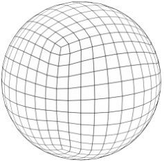
The smoothness of spline basis functions is vital in the isogeometric analysis of problems with higher-order partial differential equations. For instance, gradient-theories of elasticity and plasticity [1, 2, 3, 4, 5], phase-field modelling of sharp interfaces [6, 7, 8] and Kirchhoff-Love type plate and shell models [9, 10, 11, 12] and their extensions [13, 14] all lead to higher-order partial differential equations. Since its inception, isogeometric analysis brought about a revival of such theories mainly because of the ease of discretising higher-order partial differential equations using smooth spline basis functions. In particular, smooth basis functions avoid the introduction of (non-physical) extra degrees of freedom and promise a better integration with common computer-aided design representations. However, standard spline basis functions, including B-splines, NURBS and box-splines, are defined only on structured meshes and must be suitably extended for domains with non-trivial topology. For instance, multivariate B-splines are defined only on structured quadrilateral and hexahedral meshes in 2D and 3D, respectively. Most industrial complex geometries cannot be parametrised with a structured mesh so that a limited number of singularities on the surface or inside the volume must be introduced [15, 16, 17, 18, 19, 20, 21, 22, 23]. These singularities manifest themselves as extraordinary vertices and edges in the mesh, see Figure 1. For a hexahedral mesh, an interior vertex is extraordinary if it is not incident to hexahedra, and an interior edge is extraordinary if it is not incident to hexahedra. Similarly, an interior vertex is extraordinary for a quadrilateral mesh if it is not incident to . The construction of smooth splines which generalise or extend B-splines to unstructured meshes is currently a very active area of research in isogeometric analysis.


In computer-aided design numerous constructions have been proposed to deal with extraordinary vertices in a surface mesh, including geometrically and parametrically continuous constructions [24, 25, 26, 27, 28, 29, 30, 31, 32, 33], subdivision surfaces [34, 35, 36, 37, 38, 39, 40], macro-elements [41, 42, 43] and manifold constructions [44, 45, 46, 47, 48, 49, 50]. There is, however, a very limited number of constructions for volume meshes, including [51, 52, 53, 54, 55, 56]; most likely because conventional computer-aided design representations do not require a volume parametrisation. As widely reported, most constructions from computer-aided design do not lead in isogeometric analysis to optimally convergent finite elements, especially when applied to higher-order partial differential equations, see the discussion in [29]. There are, however, constructions for unstructured quadrilateral meshes, including [30, 32, 48, 49, 38], which yield optimal or nearly optimal convergence rates. In contrast, there are no B-spline based optimally convergent smooth constructions for unstructured hexahedral meshes. Currently, optimality is achieved by either reducing continuity to around extraordinary features [56, 57, 58], combining B-splines with meshless approximants [59] or resorting to non-standard spline definitions [60]. The first approach is not suitable for higher-order partial differential equations whereas the latter approaches lead to schemes that are usually computationally very costly.
| Terminology | Definition |
|---|---|
| Mixed B-splines, | B-splines of mixed smoothness. |
| Blending | Combination of different basis functions using weight functions. |
| SB-splines, | Smooth blended splines obtained by the proposed construction. |
In this paper, we derive a computationally efficient, easy to construct and optimally convergent extension of B-splines to unstructured quadrilateral and hexahedral meshes. We dub the new basis functions SB-splines; see Table 1 for the terminology used throughout this paper. Although we consider only quadratic B-splines, the presented ideas should carry over to arbitrary degrees. To begin with, we determine on the given unstructured mesh a set of B-splines of mixed smoothness following the construction for quadrilateral meshes presented in Toshniwal [61]. The mixed B-splines are continuous around extraordinary features, i.e. extraordinary vertices (in 2D and 3D) and extraordinary edges (in 3D), but are smooth everywhere else. Subsequently, we use the partition of unity method of Melenk and Babuška [62] to blend the mixed B-splines with tensor-product Bernstein basis functions of equal degree. To this end, a set of smooth weight, or partition of unity, functions and are defined to blend both types of basis functions. A key novelty of our approach is that the blending function is assembled from the mixed B-splines on the unstructured mesh, by excluding the ones, so that . Consequently, the weight functions and are smooth and have their breakpoints at the element boundaries. On quadrilateral meshes with extraordinary vertices the SB-splines are simply given by the weighted basis functions and . In hexahedral meshes, the extraordinary edges and vertices usually form a connected network as illustrated in Figure ; see also relevant work on hexahedral meshing [15, 16, 17, 18, 19, 20, 21, 22, 23]. That is, the weight function has a support over the entire network and is decomposed as into locally supported weight functions. In brief, the support of one weight function covers a region where more than two extraordinary edges meet, and the supports of the weight functions are restricted to the remaining regions along the connecting extraordinary edge chains. We note for blending instead of the Bernstein basis a different tensor-product basis or a triangular Bernstein-Bézier basis can be considered. Similarly, in principle, differently constructed mixed smoothness B-splines could be used, including the enhanced smoothness B-splines presented in Buchegger and Jüttler [63], which are conceptually similar to the chosen mixed B-splines. However, the enhanced smoothness B-splines use nested refinement (leading to a more involved implementation because of the mixed smoothness) and exhibit optimal convergence only for extraordinary vertices with a valence using uniform refinement.
The proposed approach uses, like the manifold-based constructions [46, 47, 48, 50, 49] and their variations [64, 65, 66, 67], the partition of unity method to smoothly blend mixed B-splines with continuous Bernstein basis functions. Unlike manifold-based constructions, the two types of basis functions are blended in the Euclidean ambient space, i.e. in 2D and in 3D. Thus, for blending we do not use an atlas consisting of charts and smooth transitions maps. Although it is easy to devise smooth transition maps for 2-manifolds, e.g. using conformal or characteristic maps [46, 36], it is not clear how to construct them in . Circumventing the need for such a smooth atlas yields a conceptually and implementation-wise simpler approach and smooth basis functions with appealing properties. The SB-splines are obtained by blending polynomials defined either on the parameter or ambient space and, hence, can be integrated very efficiently using standard Gauss-Legendre quadrature. Furthermore, the weight functions and have minimal polynomial degree considering that they are assembled from B-splines and their complements to one.
The outline of this paper is as follows. To begin with, we briefly discuss in Section 2 the construction of SB-splines in 1D to introduce the key ideas and terminology used throughout the paper. Subsequently, we consider in Section 3 the construction of SB-splines on unstructured quadrilateral meshes with extraordinary vertices. We first review the mixed B-splines in Section 3.1 and then discuss the construction of SB-splines, in particular the weight functions, in Section 3.2. As explained in Section 3.2, it is straightforward to derive closed form expressions of the new basis functions for use in existing isogeometric analysis implementations. In Section 4, we consider the construction of SB-splines on unstructured hexahedral meshes with extraordinary edges and vertices. After discussing the extension of mixed B-splines to hexahedral meshes in Section 4.1, we first introduce the notion of an extraordinary prism and extraordinary joint and discuss how to construct the respective weight and smooth basis functions in Section 4.2. Finally, we introduce in Section 5 several Poisson and biharmonic examples to confirm the convergence of the SB-splines. We study in particular the influence of the number of quadrature points and the valence of the extraordinary vertices on finite element convergence in 2D. Although we have not investigated the finite element convergence in 3D, we demonstrate the global continuity and excellent performance of the finite element solution on the same spherical domain as shown in Figure 1. The paper is supplemented by four appendices that provide a proof of linear independence and discuss aspects of finite element discretisation, mesh refinement and an illustration of the treatment of arbitrary hexahedral meshes.
2 One-dimensional SB-splines
The proposed construction is best illustrated in the one-dimensional setting. Given is a domain with the parametrisation
| (1) |
where are the univariate B-splines of degree and are the coordinates of the control points. As mentioned earlier, in higher dimensions we will focus solely on the case . The B-splines are defined on the parametric domain with the parametric coordinate . For the sake of illustration, they are chosen to be continuous at the break point and continuous at every other break point. Hence, the point with the coordinate is an extraordinary point.
Assuming that the parametrisation is, as usual, bijective, the push-forward of the basis functions on the physical domain of interest are given by
| (2) |
For later reference, the basis functions on the physical domain are collected in the array
| (3) |
In the neighbourhood of the extraordinary point , we aim to blend the B-splines with a second polynomial basis defined only over the the blending domain . The second basis is, without loss of generality, throughout this paper a Bernstein basis with the basis functions
| (4) |
where and is the polynomial degree of the Bernstein basis.
For blending together the two sets of basis functions, we choose a weight function with and its complement to one , i.e.,
| (5) |
Such weight functions can be chosen in many different ways. In the proposed construction, we assemble the weight function from the B-splines . In particular, with the index set and its complement the weight function is given by
| (6) |
The so-assembled weight functions have the following properties.
Proposition 1
The weight functions and are at least smooth, piecewise polynomials in the parameter space, have local support and form a partition of unity.
Finally, using the above set of weight and basis functions, we define the smooth blended B-splines, or SB-splines, as
| (7) |
where . Evidently, the smoothness, the support size and the polynomial degree of the SB-splines depend on the properties of , , and . Critical for the smoothness properties of the SB-splines is the choice of the weight function .
Proposition 2
The SB-splines are at least smooth, linearly independent, non-negative, have local support and form a partition of unity.
The properties of smoothness, non-negativity, local support and partition of unity follow directly from the blending construction since both and possess these properties. For the proof of linear independence, see A.
As a concrete example, Figure 3 illustrates the blending of mixed smoothness quadratic B-splines with quadratic Bernstein basis functions . The physical domain has at its centre an extraordinary point with continuity, introduced using a non-uniform open knot vector for . Except at the extraordinary point the quadratic B-spline basis is smooth. The weight function is assembled from B-splines by excluding the ones which are at most smooth at the extraordinary point. Hence, the weight function and, in turn, its complement are intrinsically smooth. The blending domain is equal to the support of the weight function . After determining the weight functions it is straightforward to compute the basis functions depicted in Figures and , which are all smooth. We emphasise that a key aspect of our construction is that the weight function is assembled from the smooth B-splines . As apparent in Figure , outside the blending region the weight function is equal to one so that the SB-splines are equal to the standard B-splines.
Evidently, the proposed construction can be applied to B-splines of any degree. Figure 3 illustrates the blending of mixed smoothness cubic B-splines and cubic Bernstein basis functions. The SB-splines depicted in Figures and are also continuous. In the next sections, we restrict our attention to .
3 Two-dimensional quadratic SB-splines
We are given an unstructured quadrilateral mesh describing a domain . The mesh consists of elements, i.e. quadrilateral faces, and their edges and vertices. We assume that all the vertices on the boundary of the mesh are regular, i.e. are adjacent to two elements, and all the extraordinary vertices within the mesh, i.e. vertices with other than four adjacent elements, are sufficiently separated as to be specified. If not the case, this can be achieved by successive quadrisection refinement of all elements. The new vertices introduced during refinement are all regular so that the extraordinary vertices become more and more separated. In the following, without loss of generality, we focus on bi-quadratic B-splines and assume that the mesh has a single extraordinary vertex of valence . In the (locally) structured regions of the mesh standard smooth tensor-product bi-quadratic B-splines can be defined. It is impossible to define such B-splines in the -neighbourhood of an extraordinary vertex due to the lack of a tensor-product mesh structure. A -neighbourhood of a vertex is formed by the union of the elements that contain the vertex. The -neighbourhood is defined recursively as the union of all 1-neighbourhoods of all the vertices in the -neighbourhood. With this definition at hand, we require that the 3-neighbourhoods of the extraordinary vertices in the considered mesh are disjoint.
3.1 Review of mixed B-splines
Although it is not possible to define a standard tensor-product B-spline basis on an unstructured mesh, it is possible to construct a B-spline basis of mixed smoothness; see Toshniwal [61]. The mixed B-splines are continuous away from the -neighbourhood of extraordinary vertices and are continuous along mesh edges adjacent to extraordinary vertices. That is, away from the -neighbourhood of extraordinary vertices the mixed B-splines are identical to tensor-product B-splines. On structured meshes there is a one-to-one correspondence between the bi-quadratic B-splines and elements (away from the boundaries). This is also the case for mixed B-splines. Hence, we can assign a control vertex to each element. The support of a mixed B-spline consists of all elements sharing a vertex with the respective element.
We represent the non-zero mixed B-splines within an element with bi-quadratic Bézier basis functions. The control vertices of the mixed B-splines are denoted with and the ones of the Bézier basis functions with . The numbering of both sets of control vertices is given in Figure . We define the mixed B-splines by first establishing the map from the control vertices to . To this end, the Bézier control vertices are expressed as linear combinations of the mixed B-spline control vertices. The corresponding weights can be graphically visualised with the masks shown in Figures and . The edge Bézier control vertices , , and are determined using the mask in Figure and the corner Bézier control vertices , , and using the mask in Figure . The centre Bézier control vertex has the same value as the mixed B-spline control vertex . Finally, the mapping of the mixed B-spline control vertices to the Bézier control vertices is given by
| (8) |
Combining the Bézier basis functions of an element with the map (8) from the control vertices to , we can define both a (local) parametrisation of the physical domain and the mixed B-splines . Note that the Bézier basis functions are local to each element. Specifically, with the mixed B-spline control vertices given in Figure and the map (8) the geometry parametrisation within the element corresponding to the control vertex is given by
| (9) |
This description also defines the mixed B-spline associated to control vertex . According to (9), its preimage in the parametric domain is given by
| (10) |
such that
| (11) |
The B-splines associated to the other control vertices in the mesh are obtained in the same way. See [61] for other properties of the mixed B-splines.
As an example, the parametrised domain, i.e. Bézier mesh corresponding to the unstructured mesh in Figure with an extraordinary vertex with is visualised in Figure . The parametrisation is smooth in most parts of the domain as is suggested by the plotted parameter lines with either or It is continuous across the edges that contain the extraordinary vertex. For a control vertex in the 1-neighbourhood of the extraordinary vertex we obtain the basis function shown in Figure . This basis function is only continuous across the edges that contain the extraordinary vertex, as can be inferred from the plotted parameter lines.

3.2 Construction of SB-splines
The construction of the blended smooth basis functions is analogous to 1D. First, we choose a weight function and its complement to one . The weight function is assembled from the smooth mixed B-splines defined on the unstructured mesh. Importantly, the blending of the basis functions takes place in the physical domain rather than the parametric domain of the basis functions. It is impossible to map every multi-dimensional physical domain with arbitrary topology onto a single parametric domain. This can be achieved only by introducing an atlas consisting of several charts with respective parametric domains and transition functions [48, 49, 50]. The definition of such smooth transition function on unstructured meshes is usually very challenging. Instead, constructing the weight functions on the physical domain sidesteps the need for an atlas and smooth transition functions.
As discussed in the preceding section smooth mixed B-splines are defined only away from the 1-neighbourhood of an extraordinary vertex. Furthermore, the mixed B-splines on the physical domain are obtained by mapping from the reference element via the mapping , see (11). According to the chain rule of differentiation the smoothness of relies both on the smoothness of and . This implies that beyond the 1-neighbourhood of an extraordinary vertex most of the control vertices in its 2-neighbourhood belong to non-smooth mixed B-splines as well, see Figure .
We assemble the weight function from the mixed B-splines by excluding the ones belonging to the control vertices in the 2-neighbourhood of the extraordinary vertex, i.e. by excluding the mixed B-splines associated to all control vertices marked with a cross or a tick in Figure . Although only the non-smooth mixed B-splines must be excluded, for ease of implementation we exclude some of the smooth mixed B-splines as well. The so-obtained smooth weight function and its complement to one are depicted in Figures and , respectively. Evidently, both weight functions are smooth, bi-quadratic on the reference element domain and is comprised of the 3-neighbourhood of the extraordinary vertex.


Next, we choose a bi-quadratic Bernstein basis as the second basis for blending. These are defined on a different domain than the ones in (9); indeed, considering that the blending takes place in the physical domain this basis is defined in the physical domain with . To guarantee the positivity of the SB-splines, the domain of the Bernstein basis must enclose the blending domain , but can be chosen freely otherwise. As in 1D, the SB-splines are then defined by
| (12) |
with
| (13) |
The obtained basis functions are smooth. In Figures and two of the basis functions and in Figure one of the basis functions are plotted.
In usual finite element implementations integrals are evaluated in a reference element domain . To facilitate the element-based implementation of the proposed blended approach, we consider a sector-wise construction of the weight functions and . The process is outlined in Figure 8. The -neighbourhood of the extraordinary vertex is partitioned into sectors. Each sector consisting of elements is parametrised with , see Figure . The elements on the parametric domain are mapped using a mapping composed of a translation and a scaling to the reference element for integration.

With the extraordinary vertex located at the origin of , the implementation of the weight functions is identical on all the sectors. Therefore, it is sufficient to detail the implementation only one of the sectors. As illustrated in Figure , the weight function is constructed by first defining on the parametric domain . We define as the tensor product of univariate weight functions and ,
| (14) |
First, we assemble along the and axes the univariate weight functions for and by excluding the univariate B-splines which are not smooth at the origin , see Figure . Then, their complements to one yield
| (15) |
For evaluating the finite element integrals the weight function values at the quadrature points in the reference element are required, which are obtained from
| (16) |
Here, the mapping is, as mentioned above, composed of a translation and scaling and can be easily inverted.
4 Three-dimensional quadratic SB-splines
The proposed construction of SB-splines can also be extended to unstructured hexahedral meshes describing a domain . A mesh consists of elements, i.e. hexahedral cells, their quadrilateral faces, edges and vertices. In 3D there are in addition to extraordinary vertices also extraordinary edges, see Figure . Extraordinary edges are connected to two extraordinary vertices and regular edges to two regular vertices. In this paper, we assume that there are no edges with one ordinary and one extraordinary vertex and that all edges on the boundary of the domain are regular, i.e. are adjacent to two elements. Furthermore, the valence of an edge is defined as the number of elements that share the same two vertices like the edge.
Well-designed hexahedral finite element meshes consist of a small number of chains of extraordinary edges. There are usually only a few extraordinary vertices with more than two attached extraordinary edges [17, 20]. As in 2D, only the 3-neighbourhood of the extraordinary vertices and extraordinary edges is relevant for the proposed construction. In 3D, the union of the 3-neighbourhoods of all the extraordinary vertices in the mesh form a 6-element wide chain of elements as depicted in Figure . We split the chain into several disjoint sets and refer to them as extraordinary prisms or extraordinary joints as illustrated in Figures and . Joints consist of the 3-neighbourhood of extraordinary vertices where more than two extraordinary edges meet. The remaining elements in the chain form the prisms. Each prism is connected to either a joint or the domain boundary.
In practice, the possible number of extraordinary edges meeting at an extraordinary vertex is limited. For the sake of clarity and conciseness, without loss of generality, we consider in this section only a joint with four attached prisms, i.e. , each of which have valence . The arbitrary and case can be similarly elaborated upon as is briefly discussed in D.


4.1 Review of mixed B-splines
We now outline the extension of the mixed B-spline construction in Section 3.1 to an unstructured hexahedral mesh. The resulting tri-quadratic mixed B-splines are continuous away from the -neighbourhood of extraordinary edges and are only continuous along mesh faces adjacent to extraordinary vertices. Again, there is a one-to-one correspondence between the tri-quadratic mixed B-splines and the elements in the mesh (away from the boundaries) so that we assign a control vertex to each element. The support of the respective mixed B-spline consists of all elements sharing a vertex with the element.
As before, we first represent the non-zero mixed B-splines within an element with tri-quadratic Bézier basis functions. Subsequently, the corresponding Bézier control vertices are expressed as linear combinations of the mixed B-spline control vertices using the masks depicted in Figure 10, the labelling of the vertices has been omitted for simplicity. The face Bézier control vertices are determined using the mask in Figure , the edge Bézier control vertices using the mask in Figure and the corner Bézier control vertices using the mask in . The masks for edge and corner Bézier control vertices depend on the valence of the edge and the valence of the vertex , respectively. The centre Bézier control vertex has the same value as the element’s respective mixed B-spline control vertex.
As in the two-dimensional case, combining the obtained Bézier basis control vertices with Bézier basis function we can define a (local) parametrisation of the physical domain as well as mixed B-splines. Recall that the parameterisation for the quadrilateral mesh in Section 3.1 was continuous across all edges adjacent to the extraordinary vertex. For hexahedral meshes the parametrisation is continuous across all faces adjacent to the extraordinary edge.
4.2 Construction of SB-splines
The construction of the blended smooth basis functions on unstructured hexahedral meshes follows the 1D and 2D constructions with only slight modification. The key idea is again to consider all the smooth mixed B-splines to define the weight function and its complement to one . A naive implementation of this idea leads on hexahedral meshes to a single weight function with a support covering all the connected extraordinary prisms and joints in the mesh. Clearly, such a construction will lead to an overly dense stiffness matrix and adversely affect the approximation properties of the SB-splines. Therefore, as will be detailed in the following, the weight function is partitioned into two sets of locally supported weight functions and such that
| (17) |
where is the number of extraordinary prisms, is the number of weight functions defined along the corresponding extraordinary prisms and is the number of extraordinary joints. In other words, there is one weight function for each extraordinary joint and several weight functions for each extraordinary prism. The construction of the prism weight functions are introduced in Section 4.2.1 and the joint weight functions in Section 4.2.2.
After the weight functions are determined, for blending we assign a tri-quadratic Bernstein basis to each weight function. In the following, the domain of each tri-quadratic Bernstein basis is assumed to be a cuboid enclosing the support of the corresponding weight function it is assigned to. We index the Bernstein basis similarly to the associated weight functions. Hence, similar to 1D and 2D, the SB-splines are defined by
| (18) |
4.2.1 Weight functions for extraordinary prisms
The weight functions for one extraordinary prism are obtained as illustrated in Figures 11 and 12. The two ends of the prism are either joined to an extraordinary joint or the boundary of the domain . The centre of the prism consists of extraordinary edges of valence . For constructing the weight functions the prism is partitioned into sectors, see Figure . Each sector consists of elements and is parametrised using with the parametric domain . The extraordinary edges are located along the parametric axis . The elements on are mapped to the reference element for integration using a mapping composed of a translation, rotation and scaling.

On a given sector of the -th prism, we define univariate weight functions from the available quadratic univariate B-splines . The number of weight functions can be chosen flexibly, as long as
- –
each is the sum of a certain number of consecutive B-splines,
- –
each has vanishing derivatives at the endpoints of its support,
- –
each B-spline is used to build exactly one , c.f. Figure ,
- –
and the sum of all is equal to 1.
For instance, in Figure the univariate weight functions are defined as
| (19) |
The isocontours of the three weight functions and their complement to one on two of the three sectors are depicted in Figure 12. Note that choosing a large ensures that the SB-splines have small support sizes.


Following the above, the trivariate weight functions are defined as the tensor product of the bivariate weight function , introduced in Section 3.2, and the univariate weight functions ,
| (20) |
The construction is repeated for all prisms to obtain weight functions for all .
4.2.2 Weight functions for extraordinary joints
Without loss of generality, we consider a single extraordinary joint with valence shared by four extraordinary prisms each of which have valence , see Figure 9, and describe the construction of its associated weight function. To simplify the construction of the extraordinary joint weight function we require that the support of the already defined prism weight functions do not overlap at the joint. Recall from the Figures 11 and 12 that the support of the prism weight functions consist in the -plane corresponds to the -neighbourhood of the extraordinary vertex. Hence, we choose the -neighbourhood of the extraordinary vertex at the centre of the joint for constructing the weight function as illustrated in Figure . At the boundary of the 3-neighbourhood, the joint meets different prisms; the intersection of the joint with each prism is composed of quadrilateral faces, with the valence of the prism’s extraordinary edge. We require that across this of faces, the values and derivatives of the weight function respectively match those of the unique prism weight function that is non-zero on all these faces. For instance, in the already discussed example in Figure the weight functions and corresponding to and have to smoothly connect to the respective joint weight functions.


To construct the joint weight function we follow once more a sector-wise approach as outlined in Figure 13. The joint is partitioned into sectors each consisting of elements. Each sector is parametrised using on the parametric domain . The extraordinary edges of the attached four prisms meet at the origin of the domain . We define the joint weight function as
| (21) | ||||
where the univariate weight functions are, as depicted in Figure , assembled from the smooth quadratic B-splines defined along the , or axes. That is,
| (22) |
In Figure 14 the isocontours of the obtained joint weight function , the weight functions of the attached four prisms and their complement to one are shown. In D we briefly demonstrate that the joint and prism weight functions for arbitrary vertex and edge valences and can be constructed following same approach.


5 Examples
We proceed to establish the finite element convergence properties and accuracy of the SB-splines in solving Poisson and biharmonic problems. The respective weak forms and the details of the finite element discretisation are summarised in B. In all the examples we use sufficiently smooth manufactured solutions and focus on quadratic basis functions, except in 1D where we also consider cubic basis functions. As known from the isogeometric analysis literature the optimal converge rates for the Poisson problem discretised with standard quadratic B-splines are and in the and (semi-)norms, respectively [68]. In contrast, the optimal convergence rates for the biharmonic problem discretised with quadratic B-splines are in the and the (semi-)norms and in the (semi-)norm [69].
5.1 One-dimensional Poisson problem
As a first example we consider the solution of a one-dimensional Poisson-Dirichlet problem on the domain . The body force is chosen such that the solution is
| (23) |
The domain is parametrised using non-uniform B-splines of degree and in turn. The knot vector and control points are selected so that each element has the same size . We intentionally introduce a continuous kink at the midspan by setting the knot multiplicity to therein. In addition, we use an open knot vector which allows the Dirichlet boundary condition to be imposed strongly.
In the following we compare the finite element convergence and the condition number of the stiffness matrices for the SB-splines with the ones for the mixed B-splines , consisting of and continuous basis functions. The continuous SB-splines are constructed by blending B-splines with Bernstein basis of same polynomial degree . In comparison to B-splines the SB-splines have the additional degrees of freedom . We begin with an initial coarse mesh of elements and obtain finer meshes using knot insertion. Figures and show that the SB-splines yield optimal convergence rates for both polynomial degrees and . In addition, the approximation error remains in the same order of magnitude with or without blending. The condition number of the respective stiffness matrices is plotted in Figure . When the mesh size is relatively large the SB-splines lead to significantly larger condition numbers than the B-splines. Interestingly, the condition numbers for SB-splines are almost independent of mesh size. Overall, the SB-splines condition numbers compare favourably with the B-splines condition numbers.
5.2 Poisson and biharmonic problems on a square domain
We consider next the Poisson-Dirichlet and biharmonic problems on a square domain . Figure 16 shows the initial semi-structured coarse mesh with extraordinary vertices. The boundary of the square domain is parametrised using open, uniform bi-quadratic B-splines. For the Poisson-Dirichlet problem, the Dirichlet boundary condition is imposed using Nitsche’s method with the stabilisation parameter chosen as , see B. For the biharmonic problem, we use the penalty approach with the stabilisation parameter chosen as . In comparison to mixed B-splines , for the SB-splines the additional degrees of freedom are . We refine the mesh using a refinement scheme described in C, so that the number of extraordinary vertices remains constant and the blending domains become increasingly smaller. In all meshes there are extraordinary vertices and in total elements in the respective blending domains.
We approximate the finite element integrals using the Gauss-Legendre quadrature rule. In order to examine the effect of the number of quadrature points on the finite element convergence, for the SB-splines , we vary for the domain integrals and use always quadrature points for the boundary integrals. For the mixed B-splines , we use for the domain integrals and boundary integrals and quadrature points, respectively.
For the two-dimensional Poisson-Dirichlet problem, the body force is chosen so that the solution is equal to
| (24) |
Figure 17 confirms that the SB-splines are optimally convergent provided that at least quadrature points are used. For , as the mesh is refined the approximation error remains in the same order of magnitude with or without blending. We conjecture that the number of quadrature points for the SB-splines to achieve the optimal convergence rate is relatively small because the weight functions and are assembled from smooth piecewise quadratic B-splines.
For the two-dimensional biharmonic problem, the body force is chosen so that the solution is equal to
| (25) |
As the mixed B-splines are not globally continuous on the considered semi-structured quadrilateral mesh, we examine only the finite element convergence using the continuous SB-splines . Figure 19 shows that the SB-splines are optimally convergent for the biharmonic problem provided that a minimum of is used for the quadrature. However, note that the relative -seminorm of error is improved using .


In addition to the convergence rate, we examine the finite element solution for the biharmonic problem qualitatively. Figure 19 shows the finite element solution and its first and second partial derivatives with respect to for the initial coarse mesh. Since the SB-splines are globally continuous, both the finite element solution and its first partial derivative with respect to are continuous as visible in Figures and , respectively. Furthermore, as known the spatial derivatives of often exhibit short-wavelength oscillations near the extraordinary vertices. Similarly, we observe such oscillations specifically for the second spatial derivatives in the blending domain as shown in Figure . However, there is no oscillation in the -neighbourhood of the extraordinary vertices.
5.3 Biharmonic problem on -gon domains
In some smooth basis function construction techniques, the respective finite element convergence rates are known to deteriorate when the valence is increased, see the discussion in [29]. Therefore, we investigate next the convergence rate of the SB-splines for different valences. To this end, we consider the biharmonic problem on five -gon domains with as depicted in Figure 20. For each domain, the extraordinary vertex is located at the global origin . The boundary is parametrised with open, uniform bi-quadratic B-splines. To impose the boundary conditions, we use the penalty approach with the stabilisation parameter chosen as . As shown to be sufficient for the biharmonic problem in Section 5.2, we use and quadrature points for approximating the domain and boundary integrals, respectively. Similarly, we refine the mesh using the refinement scheme described in C. The body force is chosen such that the solution is
| (26) |
Figure 21 shows the finite element convergence using the SB-splines . Although the convergence rates for the first few coarser meshes are slightly fluctuating, overall the SB-splines are optimally convergent. In other words, the convergence rate is identical for the considered valences . The increase of the valence leads, however, to a small increase in the convergence constants. This finding suggests that the SB-splines are robust since the studied valences are the most prevalent in well-designed meshes.
5.4 Poisson and biharmonic problems on a spherical domain
As a final example, we consider the Poisson-Dirichlet and biharmonic problems on the spherical domain in Figure 1. The spherical domain has a radius of and is centred at the global origin . As an approximation to the spherical domain, the parametrised hexahedral mesh in Figure has an average mesh size and consists of extraordinary prisms of valence and extraordinary joints. The boundary of the spherical domain is parametrised using open, uniform tri-quadratic B-splines. For the Poisson-Dirichlet problem, the Dirichlet boundary condition is imposed using Nitsche’s method with the stabilisation parameter chosen as . For the biharmonic problem, we use the penalty approach with the stabilisation parameter chosen as . The numbers of degrees of freedom for the mixed B-splines and the SB-splines are and , respectively.
For the three-dimensional Poisson-Dirichlet problem, the body force is chosen so that the solution is
| (27) |
We compare numerically the finite element solution between and . The relative -norms of error for and are and , respectively whereas the relative -seminorms of error for and are and , respectively. Therefore, the approximation error has the same order of magnitude with and without blending. Figure 22 illustrates the first partial derivative of the finite element solution with respect to . As shown in the figure, both and yield an accurate approximation to the first partial derivative of the analytical solution with respect to . In addition, Figure 23 ascertains that the SB-splines are globally continuous. For instance, the mixed B-splines yield continuous finite element solution near the extraordinary edges as inferred from the discontinuity of the first partial derivative of with respect to in Figure . In contrast, the first partial derivative of with respect to using is continuous in the same subdomains as shown in Figure .
For the three-dimensional biharmonic problem, the body force is chosen so that the solution is equal to
| (28) |
Using the SB-splines , the relative -norm of error, relative -seminorm of error and relative -seminorm of error are , and , respectively. Figure 24 shows that the SB-splines yield a satisfactory finite element approximation to the analytical solution.


6 Conclusions
We introduced SB-splines i.e. a smooth blended B-spline construction for unstructured quadrilateral and hexahedral meshes and demonstrated its optimal convergence for quadratic B-splines on unstructured quadrilateral and hexahedral meshes. We determine the smooth weight functions required for blending from the smooth mixed B-splines defined on the regular parts of the unstructured mesh. The weight functions multiplied with the available mixed B-splines and additionally introduced Bernstein basis functions yield new basis functions. As shown numerically, the SB-splines can be efficiently integrated using standard Gauss-Legendre quadrature with a very small number of quadrature points. In the blending region, the new basis functions have slightly larger support close to the extraordinary features. For instance, in 2D the support consists of the 3-neighbourhood of the extraordinary vertex. Remarkably, the numerically determined convergence rates in 2D are optimal for both Poisson and biharmonic problems and are independent of the valence of the extraordinary vertex. However, the convergence constants show a slight increase with an increase in valence, which may be explained by the short-wavelength oscillations, or ripples, in the higher-order derivatives at the blending region. As discussed, on unstructured hexahedral meshes, the extraordinary edges and vertices usually form a connected network. The respective weight functions obtained from the available smooth mixed B-splines may not have a compact support. Therefore, we decompose the weight functions so that the resulting weight functions and basis functions have a compact support and are still polynomials in the parameter space.
In closing, we stress that the proposed construction can be applied to mixed B-splines of arbitrary degrees, although we have studied only quadratic mixed B-splines so far. To this end, it is necessary to extend the introduced mesh refinement scheme for quadratic mixed B-splines to arbitrary degree. In our experience, the details of this refinement are important for achieving optimal convergence rates. For cubic SB-splines the mixed B-splines introduced in Wei et al. [56] appear as particularly promising. Moreover, while we presented some mathematical analyses (e.g., proof of linear independence in 1D), further analysis is needed to prove the numerically observed properties of SB-splines. In principle, the proposed construction can also be applied to non-uniform B-splines and extended to surfaces with arbitrary topology, i.e. 2-manifolds in . Non-uniform constructions can, amongst others, significantly simplify the enforcement of essential boundary conditions. In case of surfaces with arbitrary topology, the SB-splines have to be constructed on a set of intermediate parametric domains corresponding to each of the extraordinary vertices. The so obtained SB-splines on parametric domains can be subsequently mapped to . Lastly, to make the presented construction useful in geometric design, the introduced new degrees of freedom around the extraordinary features must be associated with control vertex positions. Following related constructions in geometric modelling, see [46, 64, 65, 67, 48], this may be achieved by projecting the new degrees of freedom to the existing or possibly some new control vertex positions in the mesh.
Appendix A Linear independence
We provide in this appendix a proof for the linear independence of the one-dimensional SB-splines. We consider as in Figures 3 and 3 a 1D setup with mixed B-splines of degree . As discussed in Section 2, we assume that the prescribed B-spline smoothness is at a single breakpoint and at all others. In general, the mixed B-splines will be non-polynomials in physical space because of the isoparametric mapping, see (2). Let denote the set of mixed B-splines , the set of Bernstein polynomials and the set of SB-splines. The set is split into the two non-intersecting sets
| (29) |
The set is composed of the three non-intersecting sets
| (30) |
As implied by the choice of weight function in (6), such that , and similarly such that . We want to prove that the functions in are linearly independent.
Linear independence requires that
| (31) |
is satisfied only when the coefficients . Observe that outside the blending domain, (31) reduces to
| (32) |
Therefore, due to the linear independence of B-splines, we obtain for all . The remaining terms in (31) correspond to splines with a support inside the blending region . We prove by contradiction that the coefficients of the non-vanishing terms must be zeros. Assume that the SB-splines are linearly dependent such that
| (33) |
or equivalently that
| (34) |
Next, observe that there are two elements such that on each there is only one function from that is non-zero, e.g., the leftmost or the rightmost element in the grey region in Figure 3 or Figure 3. Let the corresponding non-zero functions be , respectively. Then, we have and , , thus
| (35) |
Note that the right hand side is a polynomial function.
- –
Case 1: Let be non-polynomial. Then, the equality in (35) can be satisfied only if both sides are equal to .
- –
Case 2: Let the isoparametric mapping be such that both are obtained by affinely mapping the associated element in parameter space. Thus, are degree polynomials for both . This has two implications. First, for equality, both the left and right hand sides in (35) need to represent the same polynomial, say , of degree . Note that is thus a global polynomial on . Second, by the end-point vanishing property of B-splines, vanishes times on one of the endpoints of , . This imposes constraints on the polynomial , thus implying .
Both the above cases imply that the right hand side in (35) is zero and, in particular, all coefficients of are thus zero by their linear independence. As a result, the right hand side in (34) is zero, thus implying that all coefficients of are zero by their linear independence.
Appendix B Finite element discretisation
B.1 Poisson equation
The Poisson equation is given by
| (36) |
where is the solution field in the domain due to the body force , is the prescribed solution field on the Dirichlet boundary , is the prescribed flux on the Neumann boundary with the outward unit normal , is the gradient operator and is the Laplacian operator. The weak formulation of the Poisson equation can be stated as [70, 71]: Find such that
| (37) |
for all with
| (38a) | ||||
| (38b) | ||||
and the positive stabilisation parameter .
B.2 Biharmonic equation
The biharmonic equation is given by
| (39) |
where and are respectively the bending moment and shear force prescribed on the Neumann boundary . The weak formulation of the biharmonic equation can be stated as [72]: Find such that
| (40) |
for all where
| (41a) | ||||
| (41b) | ||||
B.3 Finite element discretisation
We discretise the trial and test functions with the SB-splines as
| (42) |
Introducing the interpolation equation (42) into the weak form of Poisson equation (37) or biharmonic equation (40) yields a system of linear equations with the unknowns . For instance, the bilinear form for the Poisson equation becomes after discretisation
| (43) |
As usual, the domain integral is evaluated numerically after splitting it into element contributions
| (44) |
Appendix C Mesh refinement
We use for the unstructured quadrilateral mesh the non-nested refinement scheme by Toshniwal [61]. Given a set of mixed B-spline control vertices from the coarse Bézier mesh, the objective is to obtain a new set of mixed B-spline control vertices for defining the refined Bézier mesh. Away from the -neighbourhood of an extraordinary vertex, that is, where a tensor product structure is locally present, the knot insertion algorithm is used. The refinement of the -neighbourhood of an extraordinary vertex of valence consists of three steps shown in Figure 25. First, the mixed B-spline control vertices at the -neighbourhood of the refined Bézier mesh are obtained from the knot insertion algorithm as shown in Figure . As a result, only the mixed B-spline control vertices at the -neighbourhood of the refined Bézier mesh remain to be selected. In particular, the remaining mixed B-spline control vertices are selected such that the midpoints of the edges at the -neighbourhood of the coarse Bézier mesh are interpolated. Therefore, the second step is to estimate the midpoints shown in Figure using, for instance, a root-finding algorithm together with a parametrisation for the edge length. Subsequently, in the third step a linear system of equations is solved for the mixed B-spline control vertices at the -neighbourhood of the refined Bézier mesh shown in Figure .
The linear system is invertible for the case of odd valences but not the case of even valences . For even valences, the linear system has a rank of . For the case of even valences, following [61] we constrain of the mixed B-spline control vertices so that the linear system has a unique solution. Evidently, the choice of the constrained mixed B-spline control vertex is not arbitrary. For instance, choosing to constraint a mixed B-spline control vertex that is far away from the extraordinary vertex can distort the refined Bézier mesh. To avoid any mesh distortion, in this paper, we first select of the extraordinary elements from the coarse Bézier mesh. After that, assuming that the extraordinary vertex is located at the reference element origin of the selected extraordinary element, we constrain the mixed B-spline control vertex at where and are decided case by case, i.e. depending on the coarse Bézier mesh. For example, in Section 5.3, we observe that the choice of with generally preserves the mesh quality after refinement.
Appendix D Arbitrary joint and prism valences
We briefly demonstrate that the approach discussed in Section 4.2.2 applies to an extraordinary joint with arbitrary edge valences and vertex valence . As a concrete example, Figure 26 illustrates the construction of weight functions for an unstructured hexahedral mesh of a truncated box domain with a spherical cavity. The unstructured hexahedral mesh shown in consists of one set of extraordinary edges of valence and three sets of extraordinary edges of valence shown in . The valences of the extraordinary edges can be verified from the extraordinary hexahedra of the mesh shown in . Overall, the unstructured hexahedral mesh consists of an extraordinary joint where the extraordinary edges of valence and meet at a vertex of valence . As discussed in Section 4.2.2, we first require that the support of the prism weight functions do not overlap at the extraordinary joint, see Figure depicting the union of the prism weight function supports. Subsequently, the extraordinary joint weight function is defined over the set of hexahedra in Figure . Conceptually, the extraordinary joint weight function defined over the set of hexahedra in Figure resembles that shown in Figure .



References
- Fischer et al. [2011] P. Fischer, M. Klassen, J. Mergheim, P. Steinmann, R. Müller, Isogeometric analysis of 2D gradient elasticity, Computational Mechanics 47 (3) (2011) 325–334.
- Rudraraju et al. [2014] S. Rudraraju, A. Van der Ven, K. Garikipati, Three-dimensional isogeometric solutions to general boundary value problems of Toupin’s gradient elasticity theory at finite strains, Computer Methods in Applied Mechanics and Engineering 278 (2014) 705–728.
- Niiranen et al. [2016] J. Niiranen, S. Khakalo, V. Balobanov, A. H. Niemi, Variational formulation and isogeometric analysis for fourth-order boundary value problems of gradient-elastic bar and plane strain/stress problems, Computer Methods in Applied Mechanics and Engineering 308 (2016) 182–211.
- de Borst and Verhoosel [2016] R. de Borst, C. V. Verhoosel, Gradient damage vs phase-field approaches for fracture: Similarities and differences, Computer Methods in Applied Mechanics and Engineering 312 (2016) 78–94.
- Codony et al. [2019] D. Codony, O. Marco, S. Fernández-Méndez, I. Arias, An immersed boundary hierarchical B-spline method for flexoelectricity, Computer Methods in Applied Mechanics and Engineering 354 (2019) 750–782.
- Gómez et al. [2008] H. Gómez, V. M. Calo, Y. Bazilevs, T. J. R. Hughes, Isogeometric analysis of the Cahn–Hilliard phase-field model, Computer Methods in Applied Mechanics and Engineering 197 (2008) 4333–4352.
- Dedè et al. [2012] L. Dedè, M. J. Borden, T. J. R. Hughes, Isogeometric analysis for topology optimization with a phase field model, Archives of Computational Methods in Engineering 19 (2012) 427–465.
- Liu et al. [2013] J. Liu, L. Dede, J. A. Evans, M. J. Borden, T. J. R. Hughes, Isogeometric analysis of the advective Cahn–Hilliard equation: spinodal decomposition under shear flow, Journal of Computational Physics 242 (2013) 321–350.
- Cirak et al. [2000] F. Cirak, M. Ortiz, P. Schröder, Subdivision surfaces: A new paradigm for thin-shell finite-element analysis, International Journal for Numerical Methods in Engineering 47 (2000) 2039–2072.
- Kiendl et al. [2009] J. Kiendl, K.-U. Bletzinger, J. Linhard, R. Wüchner, Isogeometric shell analysis with Kirchhoff–Love elements, Computer Methods in Applied Mechanics and Engineering 198 (2009) 3902–3914.
- Benson et al. [2011] D. J. Benson, Y. Bazilevs, M.-C. Hsu, T. J. R. Hughes, A large deformation, rotation-free, isogeometric shell, Computer Methods in Applied Mechanics and Engineering 200 (13-16) (2011) 1367–1378.
- Bartezzaghi et al. [2015] A. Bartezzaghi, L. Dedè, A. Quarteroni, Isogeometric analysis of high order partial differential equations on surfaces, Computer Methods in Applied Mechanics and Engineering 295 (2015) 446–469.
- Long et al. [2012] Q. Long, P. B. Bornemann, F. Cirak, Shear-flexible subdivision shells, International Journal for Numerical Methods in Engineering 90 (2012) 1549–1577.
- Echter et al. [2013] R. Echter, B. Oesterle, M. Bischoff, A hierarchic family of isogeometric shell finite elements, Computer Methods in Applied Mechanics and Engineering 254 (2013) 170–180.
- Murdoch et al. [1997] P. Murdoch, S. Benzley, T. Blacker, S. A. Mitchell, The spatial twist continuum: A connectivity based method for representing all-hexahedral finite element meshes, Finite Elements in Analysis and Design 28 (2) (1997) 137–149.
- Tarini et al. [2004] M. Tarini, K. Hormann, P. Cignoni, C. Montani, Polycube-maps, ACM Transactions on Graphics (TOG) 23 (3) (2004) 853–860.
- Nieser et al. [2011] M. Nieser, U. Reitebuch, K. Polthier, CubeCover–parameterization of 3D volumes, Computer Graphics Forum 30 (2011) 1397–1406.
- Shepherd and Johnson [2008] J. F. Shepherd, C. R. Johnson, Hexahedral mesh generation constraints, Engineering with Computers 24 (3) (2008) 195–213.
- Li et al. [2012] Y. Li, Y. Liu, W. Xu, W. Wang, B. Guo, All-hex meshing using singularity-restricted field, ACM Transactions on Graphics (TOG) 31 (2012) 1–11.
- Zhang [2018] Y. J. Zhang, Geometric modeling and mesh generation from scanned images, Chapman and Hall/CRC, 2018.
- Bracci et al. [2019] M. Bracci, M. Tarini, N. Pietroni, M. Livesu, P. Cignoni, HexaLab.net: An online viewer for hexahedral meshes, Computer-Aided Design 110 (2019) 24–36.
- Zhang et al. [2020] P. Zhang, J. Vekhter, E. Chien, D. Bommes, E. Vouga, J. Solomon, Octahedral Frames for Feature-Aligned Cross Fields, ACM Transactions on Graphics (TOG) 39 (3) (2020) 1–13.
- Livesu et al. [2020] M. Livesu, N. Pietroni, E. Puppo, A. Sheffer, P. Cignoni, LoopyCuts: practical feature-preserving block decomposition for strongly hex-dominant meshing, ACM Transactions on Graphics (TOG) 39 (4) (2020) 121–1.
- DeRose [1990] T. D. DeRose, Necessary and sufficient conditions for tangent plane continuity of Bézier surfaces, Computer Aided Geometric Design 7 (1-4) (1990) 165–179.
- Reif [1998] U. Reif, TURBS—topologically unrestricted rational B-splines, Constructive Approximation 14 (1998) 57–77.
- Scott et al. [2014] M. A. Scott, D. C. Thomas, E. J. Evans, Isogeometric spline forests, Computer Methods in Applied Mechanics and Engineering 269 (2014) 222–264.
- Nguyen et al. [2016] T. Nguyen, K. Karčiauskas, J. Peters, finite elements on non-tensor-product 2D and 3D manifolds, Applied Mathematics and Computation 272 (2016) 148–158.
- Collin et al. [2016] A. Collin, G. Sangalli, T. Takacs, Analysis-suitable multi-patch parametrizations for isogeometric spaces, Computer Aided Geometric Design 47 (2016) 93–113.
- Toshniwal et al. [2017a] D. Toshniwal, H. Speleers, T. J. R. Hughes, Smooth cubic spline spaces on unstructured quadrilateral meshes with particular emphasis on extraordinary points: Geometric design and isogeometric analysis considerations, Computer Methods in Applied Mechanics and Engineering 327 (2017a) 411–458.
- Toshniwal et al. [2017b] D. Toshniwal, H. Speleers, R. R. Hiemstra, T. J. R. Hughes, Multi-degree smooth polar splines: A framework for geometric modeling and isogeometric analysis, Computer Methods in Applied Mechanics and Engineering 316 (2017b) 1005–1061.
- Kapl et al. [2017] M. Kapl, F. Buchegger, M. Bercovier, B. Jüttler, Isogeometric analysis with geometrically continuous functions on planar multi-patch geometries, Computer Methods in Applied Mechanics and Engineering 316 (2017) 209–234.
- Kapl et al. [2018] M. Kapl, G. Sangalli, T. Takacs, Construction of analysis-suitable planar multi-patch parameterizations, Computer-Aided Design 97 (2018) 41–55.
- Karčiauskas and Peters [2021] K. Karčiauskas, J. Peters, Multi-sided completion of bi-3 and bi-2 splines: A unifying approach, Computer Aided Geometric Design 86 (2021) 101978.
- Doo and Sabin [1978] D. Doo, M. Sabin, Behavior of recursive division surfaces near extraordinary points, Computer-Aided Design 10 (1978) 356–360.
- Catmull and Clark [1978] E. Catmull, J. Clark, Recursively generated B-spline surfaces on arbitrary topological meshes, Computer-Aided Design 10 (1978) 350–355.
- Peters and Reif [2008] J. Peters, U. Reif, Subdivision Surfaces, Springer, 2008.
- Wei et al. [2015] X. Wei, Y. J. Zhang, T. J. R. Hughes, M. A. Scott, Truncated hierarchical Catmull–Clark subdivision with local refinement, Computer Methods in Applied Mechanics and Engineering 291 (2015) 1–20.
- Wei et al. [2021] X. Wei, X. Li, Y. J. Zhang, T. J. R. Hughes, Tuned hybrid nonuniform subdivision surfaces with optimal convergence rates, International Journal for Numerical Methods in Engineering 122 (9) (2021) 2117–2144.
- Zhang et al. [2018a] Q. Zhang, M. Sabin, F. Cirak, Subdivision surfaces with isogeometric analysis adapted refinement weights, Computer-Aided Design 102 (2018a) 104–114.
- Ma and Ma [2019] Y. Ma, W. Ma, A subdivision scheme for unstructured quadrilateral meshes with improved convergence rate for isogeometric analysis, Graphical Models 106 (2019) 101043.
- Clough and Tocher [1965] R. Clough, J. Tocher, Finite element stiffness matricess for analysis of plate bending, in: Proceedings of the Conference on Matrix Methods in Structuraly Analysis, 515–546, 1965.
- Powell and Sabin [1977] M. J. D. Powell, M. A. Sabin, Piecewise quadratic approximations on triangles, ACM Transactions on Mathematical Software 3 (1977) 316–325.
- Lai and Schumaker [2007] M.-J. Lai, L. L. Schumaker, Spline functions on triangulations, vol. 110, Cambridge University Press, 2007.
- Grimm and Hughes [1995] C. M. Grimm, J. F. Hughes, Modeling surfaces of arbitrary topology using manifolds, in: SIGGRAPH 1995 Conference Proceedings, 359–368, 1995.
- Della Vecchia et al. [2008] G. Della Vecchia, B. Jüttler, M.-S. Kim, A construction of rational manifold surfaces of arbitrary topology and smoothness from triangular meshes, Computer Aided Geometric Design 25 (2008) 801–815.
- Ying and Zorin [2004] L. Ying, D. Zorin, A simple manifold-based construction of surfaces of arbitrary smoothness, ACM Transactions on Graphics (TOG) 23 (2004) 271–275.
- Tosun and Zorin [2011] E. Tosun, D. Zorin, Manifold-based surfaces with boundaries, Computer Aided Geometric Design 28 (2011) 1–22.
- Majeed and Cirak [2017] M. Majeed, F. Cirak, Isogeometric analysis using manifold-based smooth basis functions, Computer Methods in Applied Mechanics and Engineering 316 (2017) 547–567.
- Zhang and Cirak [2020] Q. Zhang, F. Cirak, Manifold-based isogeometric analysis basis functions with prescribed sharp features, Computer Methods in Applied Mechanics and Engineering 359 (2020) 112659.
- Zhang et al. [2018b] Q. Zhang, T. Takacs, F. Cirak, Manifold-based B-splines on unstructured meshes, in: Conference on Isogeometric Analysis and Applications, Springer, 243–262, 2018b.
- Bajaj et al. [2002] C. Bajaj, S. Schaefer, J. Warren, G. Xu, A subdivision scheme for hexahedral meshes, The Visual Computer 18 (2002) 343–356.
- Chang et al. [2002] Y.-S. Chang, K. T. McDonnell, H. Qin, A new solid subdivision scheme based on box splines, in: Proceedings of the Seventh ACM Symposium on Solid Modeling and Applications, 226–233, 2002.
- Xie et al. [2020] J. Xie, J. Xu, Z. Dong, G. Xu, C. Deng, B. Mourrain, Y. J. Zhang, Interpolatory Catmull-Clark volumetric subdivision over unstructured hexahedral meshes for modeling and simulation applications, Computer Aided Geometric Design 80 (2020) 101867:1–101867:16.
- Reif and Sabin [2019] U. Reif, M. A. Sabin, Old problems and new challenges in subdivision, Journal of Computational and Applied Mathematics 349 (2019) 523–531.
- Peters [2020] J. Peters, Refinable tri-variate splines for box-complexes including irregular points and irregular edges, Computer Aided Geometric Design 80 (2020) 101877.
- Wei et al. [2018] X. Wei, Y. J. Zhang, D. Toshniwal, H. Speleers, X. Li, C. Manni, J. A. Evans, T. J. R. Hughes, Blended B-spline construction on unstructured quadrilateral and hexahedral meshes with optimal convergence rates in isogeometric analysis, Computer Methods in Applied Mechanics and Engineering 341 (2018) 609–639.
- Schneider et al. [2019] T. Schneider, J. Dumas, X. Gao, M. Botsch, D. Panozzo, D. Zorin, Poly-spline finite-element method, ACM Transactions on Graphics (TOG) 38 (3) (2019) 1–16.
- Schneider et al. [2021] T. Schneider, D. Panozzo, X. Zhou, Isogeometric high order mesh generation, Computer Methods in Applied Mechanics and Engineering 386 (2021) 114104.
- Wang and Zhang [2014] D. Wang, H. Zhang, A consistently coupled isogeometric–meshfree method, Computer Methods in Applied Mechanics and Engineering 268 (2014) 843–870.
- Febrianto et al. [2021] E. Febrianto, M. Ortiz, F. Cirak, Mollified finite element approximants of arbitrary order and smoothness, Computer Methods in Applied Mechanics and Engineering 373 (2021) 113513.
- Toshniwal [2022] D. Toshniwal, Quadratic splines on quad-tri meshes: Construction and an application to simulations on watertight reconstructions of trimmed surfaces, Computer Methods in Applied Mechanics and Engineering 388 (2022) 114174.
- Melenk and Babuška [1996] J. M. Melenk, I. Babuška, The partition of unity finite element method: basic theory and applications, Computer Methods in Applied Mechanics and Engineering 139 (1996) 289–314.
- Buchegger et al. [2016] F. Buchegger, B. Jüttler, A. Mantzaflaris, Adaptively refined multi-patch B-splines with enhanced smoothness, Applied Mathematics and Computation 272 (2016) 159–172.
- Zorin [2006] D. Zorin, Constructing curvature-continuous surfaces by blending, in: Proceedings of the fourth Eurographics Symposium on Geometry Processing, 31–40, 2006.
- Levin [2006] A. Levin, Modified subdivision surfaces with continuous curvature, in: SIGGRAPH 2006 Conference Proceedings, 1035–1040, 2006.
- Pla-Garcia et al. [2006] N. Pla-Garcia, M. Vigo-Anglada, J. Cotrina-Navau, N-sided patches with B-spline boundaries, Computers & Graphics 30 (2006) 959–970.
- Antonelli et al. [2013] M. Antonelli, C. V. Beccari, G. Casciola, R. Ciarloni, S. Morigi, Subdivision surfaces integrated in a CAD system, Computer-Aided Design 45 (2013) 1294–1305.
- Bazilevs et al. [2006] Y. Bazilevs, L. Beirao de Veiga, J. A. Cottrell, T. J. R. Hughes, G. Sangalli, Isogeometic analysis: approximation, stability and error estimates for h-refined meshes, Mathematical Methods and Models in Applied Sciences 16 (2006) 1031–1090.
- Tagliabue et al. [2014] A. Tagliabue, L. Dedè, A. Quarteroni, Isogeometric analysis and error estimates for high order partial differential equations in fluid dynamics, Computers & Fluids 102 (2014) 277–303.
- Nitsche [1971] J. Nitsche, Über ein Variationsprinzip zur Lösung von Dirichlet-Problemen bei Verwendung von Teilräumen, die keinen Randbedingungen unterworfen sind, Abhandlungen aus dem Mathematischen Seminar der Universität Hamburg 36 (1971) 9–15.
- Fernandez-Mendez and Huerta [2004] S. Fernandez-Mendez, A. Huerta, Imposing essential boundary conditions in mesh-free methods, Computer Methods in Applied Mechanics and Engineering 193 (2004) 1257–1275.
- Embar et al. [2010] A. Embar, J. Dolbow, I. Harari, Imposing Dirichlet boundary conditions with Nitsche’s method and spline-based finite elements, International Journal for Numerical Methods in Engineering 83 (7) (2010) 877–898.