myctr
STATISTICAL PROPERTIES OF RANKINGS IN SPORTS AND GAMES
Abstract
Any collection can be ranked. Sports and games are common examples of ranked systems: players and teams are constantly ranked using different methods. The statistical properties of rankings have been studied for almost a century in a variety of fields. More recently, data availability has allowed us to study rank dynamics: how elements of a ranking change in time. Here, we study the rank distributions and rank dynamics of twelve datasets from different sports and games. To study rank dynamics, we consider measures we have defined previously: rank diversity, change probability, rank entropy, and rank complexity. We also introduce a new measure that we call “system closure” that reflects how many elements enter or leave the rankings in time. We use a random walk model to reproduce the observed rank dynamics, showing that a simple mechanism can generate similar statistical properties as the ones observed in the datasets. Our results show that, while rank distributions vary considerably for different rankings, rank dynamics have similar behaviors, independently of the nature and competitiveness of the sport or game and its ranking method. Our results also suggest that our measures of rank dynamics are general and applicable for complex systems of different natures.
keywords
ranking; dynamics; sports; success; competition.1 Introduction
Ranking in sports has been a common instrument to classify players and teams. The best team or player is given rank , the second one has , and so on. In each sport, different rules are used to rank, as we show here with two examples. We first mention the FIFA ranking of national football teams. This uses the Elo method [12], that adds or subtracts points for individual matches from a team’s existing point total. If denotes the points a team has before a given match, the new number of points is obtained adding to the quantity . The value of varies between 5 and 60 according to the importance of the match, is the result of the match (being equal to 1 if the team wins, 0.5 for a draw and 0 if the team is defeated), and refers to the expected result of the match; the FIFA classification uses the formula with equal to the difference in of the two teams. As a second example, we refer to the ranking used by the Global Poker Index (GPI) [27]. In this case, only tournaments open to the public are taken into account if they fulfill the following characteristics: at least 32 players participate, bets must be larger than 1 dollar, and the tournament should have taken place within the 36 months before the ranking was made. The score obtained by each player is calculated according to the position obtained in the tournaments and the amount of money earned. Older tournaments have a higher weight. These two examples illustrate how rankings can be constructed. Beyond sports, an arbitrary variable can be used to order a set of elements into a ranking.
Less attention has been given to the way rank evolves in time. Still, with the recent data availability, studies of rank dynamics began to appear [3, 5, 14, 24]. A few years ago, the first complex system we investigated [7] was related to languages and the time evolution of word usage was characterized by the rank diversity, which is equal to the number of different words with rank in a time interval . This analysis was extended in [21] to the case of -grams, that is, groups of words. In order to understand the hierarchical formation of word usage, George Zipf [32, 10] proposed that the frequency of a word is related to the word rank as . This is known as Zipf’s law and is an example of a rank distribution. In [22] several complex systems sports and games were considered. The disciplines we took into account were football (national teams and clubs), golf and tennis (for male competitors) as well as poker and chess. In all cases we considered the distribution of scores versus ranks, that is, the rank distribution version for these systems, a generalization of the Zipf’s law to the context of sports and games. The rank diversity, which is equal to the number of different players or teams with rank in a time interval , was also calculated. The random walker model introduced previously [7] was used to obtain the observed rank properties. The rank distributions differs according to the sport, game or language discussed, but in all cases the rank diversity was found to be a log-normal distribution.
In this paper, the analysis of sports and games is extended, considering now twelve different cases, see Table 1. Besides the rank diversity, we also obtain for games and sports the rank change probability, the rank entropy and the rank complexity previously studied for -grams [21]. We also use the random walker model to fit the rank diversity data.
| Sport/game | Data Source | Time Period | Timescale | #players/teams |
|---|---|---|---|---|
|
Chess players*
(female) |
Fédération Internationale des Échecs (FIDE-F) [11] | Jul 2012 – Apr 2016 | Monthly | 12681 |
|
Chess players
(male) |
Fédération Internationale des Échecs (FIDE-M) [11] | Jul 2012 – Apr 2016 | Monthly | 13500 |
| Football teams |
Football Club World
Ranking (FCWR-C) [8] |
Feb 1st, 2012 –
Dec 29th, 2014 |
Weekly | 850 |
| National football teams |
Fédération Internationale de Football Association
(FIFA) [12] |
Jul 2010 – Dec 2015 | Monthly | 150 |
| Football Scorers in Clubs* |
Football Club World
Ranking (FCWR-G) [8] |
Week 33, 2016 –
Week 33 2017 |
Weekly | 400 |
| Golf players | Official World Golf Ranking (OWGR) [16] |
Sept 10th, 2000 –
Apr 19th, 2015 |
Weekly | 1000 |
|
Racers in the
Busch Grand Nation Tournament* |
National Association for Stock Car Auto Racing (NASCAR-B) [23] | 1982 – 2015 | Annual | 76 |
|
Racers in the
Winston Cup Grand National Tournament* |
National Association for Stock Car Auto Racing (NASCAR-W) [23] | 1979 – 2013 | Annual | 50 |
| Poker players |
Global Poker Index
(GPI) [27] |
Jul 25th, 2012 –
Jun 10th, 2015 |
Weekly | 1799 |
| Snowboard riders* |
World Snowboarding
(WSD) [29] |
January 5th, 2015 – March 26th, 2018 | Weekly | 1413 |
|
Tennis players
(male) |
Association of Tennis
Professionals (ATP) [1] |
May 5th, 2003 –
Dec 27th, 2010 |
Weekly | 1600 |
| Videogame earnings* |
E-Sports Earnings
(ESE) [30] |
2003 – 2016 | Annual | 400 |
2 Rank Distribution
Considering birth and death processes, we obtained in reference [7] four generalizations of Zipf’s law:
| (1) |
| (2) |
a fifth model given by the double Zipf law [14],
| (3) |
was also taken into account.
Here is the number of words considered, is a normalization constant, , , and are parameters to be fixed fitting the data. is Zipf’s law, a power law distribution. If plotted in scale, it is a straight line with steepness . and are called in the literature the gamma and beta distributions, respectively, while is a combination of both. In the linguistic case, Gerlach and Altman [14] introduced model which is the concatenation of two power laws, one corresponding to words which have high frequency and the other to those with low frequency. To find out which distribution fits the data better, we shall use two coefficients: the coefficient of determination [19] and the Kolmogorov-Smirnov index [18, 6], which is only applicable when dealing with probability distributions, this being our case. The closer is to unity, the model fits the data better. On the other hand, when the model can be discarded.
The comparisons of the five models with the observed data are shown for the twelve sports and games in Fig. 1. The data correspond to the following time slices: FIDE-F (April 2016), FIDE-M (April 2016), FCWR-C (week 53 of 2014), FIFA (June 2017), FCWR-G (week 33 of 2017), OWGR(May 21st of 2017), NASCAR-B (2015), NASCAR-W (2013), GPI (May 31st of 2017), WSD (April 26, 2018), ATP (December 27, 2010), and ESE (2016). The values of the parameters of the different distributions that fit the data better are given in Table 2.

| Model | Model | Model | ||||||
|---|---|---|---|---|---|---|---|---|
| FIDE-F | ||||||||
| FIDE-M | ||||||||
| FCWR-C | ||||||||
| FIFA | ||||||||
| FCWR-G | ||||||||
| OWGR | ||||||||
| NASCAR-B | ||||||||
| NASCAR-W | ||||||||
| GPI | ||||||||
| WSD | ||||||||
| ATP | ||||||||
| ESE | ||||||||
| Model | Model | |||||||
|---|---|---|---|---|---|---|---|---|
| FIDE-F | ||||||||
| FIDE-M | ||||||||
| FCWR-C | ||||||||
| FIFA | ||||||||
| FCWR-G | ||||||||
| OWGR | ||||||||
| NASCAR-B | ||||||||
| NASCAR-W | ||||||||
| GPI | ||||||||
| WSD | ||||||||
| ATP | ||||||||
| ESE | ||||||||
The average values, taken over all time slices available of and the standard deviation are given in Table 3. None of the distributions fit the data for all sports and games; in particular, Zipf’s law () is never the best. Furthermore, using the values of the time average of the Kolmogorov-Smirnov index , also given in Table 3, one can conclude that Zipf’s law can be discarded. From the data for FIDE-F, FIDE-M, FCWR-C and GPI, one can see that none of the models describes the way scores are distributed. We should also mention that when models or work, so does model . If model is acceptable, as for FIFA and NASCAR-W, one can conclude that for large values of the distribution falls abruptly, indicating that the less able competitors receive a very small amount of points from these federations compared to those given to the competitors who had the best performance. When the double Zipf model is adequate, as for FCWR-G, NASCAR-B, NASCAR-W, ATP and ESE, there exist two independent regimes characterized by the exponent of the power laws. The first regime corresponds to the better competitors and the second one to those with poor performance. As mentioned in reference [14], those belonging to the second regime do not affect the rank of the competitors in the first regime.
In Table 3, some models have index values below the threshold 0.1 while still having a high . This is because quantifies whether a dataset has a distribution similar to a model , while only measures how good a dataset fits a function defined by . Thus, if most data points fall close to , will be high. However, if the distribution of those points is not close to the one expected by , then .
| FIDE-F | 0.4450.047 | 0.9810.016 | 0.890.031 | 0.9950.002 | 0.9650.011 | |
|---|---|---|---|---|---|---|
| 0.00.0 | 0.00.0 | 0.00.0 | 0.00.0 | 0.0360.004 | ||
| FIDE-M | 0.7780.007 | 0.9360.005 | 0.6570.017 | 0.9360.005 | 0.9910.001 | |
| 0.00.0 | 0.00.0 | 0.00.0 | 0.00.0 | 0.0010.001 | ||
| FCWR-C | 0.7270.028 | 0.9870.005 | 0.9820.005 | 0.9970.001 | 0.9480.01 | |
| 0.0020.002 | 0.00.0 | 0.0140.017 | 0.0020.006 | 0.0010.001 | ||
| FIFA | 0.7630.021 | 0.9870.004 | 0.9930.004 | 0.9970.001 | 0.970.005 | |
| 0.00.0 | 0.0110.012 | 0.4150.32 | 0.4880.351 | 0.0740.038 | ||
| FCWR-G | 0.9730.013 | 0.9920.003 | 0.9850.006 | 0.9920.003 | 0.9920.002 | |
| 0.0470.071 | 0.7590.234 | 0.0320.052 | 0.7410.229 | 0.3170.206 | ||
| OWGR | 0.650.132 | 0.9850.014 | 0.9710.011 | 0.9850.012 | 0.9720.009 | |
| 0.00.0 | 0.6120.242 | 0.00.0 | 0.5270.337 | 0.0930.157 | ||
| NASCAR-B | 0.3920.218 | 0.9710.017 | 0.8530.068 | 0.9740.015 | 0.9760.013 | |
| 0.0010.002 | 0.3320.293 | 0.0080.025 | 0.2990.293 | 0.2580.226 | ||
| NASCAR-W | 0.4690.162 | 0.8450.068 | 0.9520.022 | 0.950.025 | 0.9320.066 | |
| 0.0210.024 | 0.0050.018 | 0.1530.24 | 0.1240.192 | 0.1890.16 | ||
| GPI | 0.7960.014 | 0.9770.005 | 0.9380.005 | 0.9770.005 | 0.9820.007 | |
| 0.00.0 | 0.00.0 | 0.00.0 | 0.00.0 | 0.00.001 | ||
| WSD | 0.7990.016 | 0.9890.003 | 0.9540.006 | 0.9890.003 | 0.9720.004 | |
| 0.00.0 | 0.1150.148 | 0.00.0 | 0.1180.154 | 0.00.0 | ||
| ATP | 0.2720.211 | 0.9820.013 | 0.880.067 | 0.9820.013 | 0.9650.029 | |
| 0.0010.003 | 0.4330.232 | 0.00.0 | 0.5930.411 | 0.1060.11 | ||
| ESE | 0.8260.104 | 0.940.043 | 0.9030.06 | 0.9190.105 | 0.9650.037 | |
| 0.0180.026 | 0.0740.11 | 0.0230.056 | 0.0640.112 | 0.1680.243 |
3 Rank Dynamics
We shall now study the time evolution of the rank occupancy. In Fig. 2 we plot as a function of time for the top 8 football clubs. These so-called ’spaghetti’ curves show how elements — individuals or teams — change their rank in time. Fig. 3 shows more detailed spaghetti curves. In several, the following behavior is observed: low ranks change less than higher ranks. In other words, change of the best is slower than that of the rest. However, this is less clear for other sports. Since a purely visual inspection might be misleading, a more formal measure is desirable.


For this purpose, we can calculate the rank diversity introduced recently [7]. If for each sport or game we have ranking information for times , we define as the element (player or team) with rank at time . If we denote by the set of elements that have rank at all times, the rank diversity is defined as:
| (4) |
where is the cardinality of the set . Notice that diversity will range from (when for a given rank, elements are different for each time step) to 1 (when only one element occupies a given rank). For example, for the data presented in figure 2, , , and . The rank diversity for several sports and games is presented in figure 4 (left).
We will now introduce what we shall call the system closure, defined below. If the elements of the system are always the same we will say that the system is closed. This happens, for example, for the classification of football national teams: few countries enter and leave the rankings, as most teams are always considered. To quantify closure we will introduce the closure index . Let us consider an arbitrary integer and take into account only those elements with ranking between and We denote by the number of elements that at time had a rank smaller than ; therefore, . In other words, is the size of the ranking, e.g., for the “top 100”, , while indicates how many elements have passed through the ranking during time . The closure index is then
| (5) |
When all elements are the same for all times, the system is completely closed and , i.e., all elements are in the ranking at all times. If, on the other hand, competitors or teams enter or leave the ranking with time, grows and decreases. Therefore, the closure index indicates how closed the system is. In Fig. 4 the values of for the twelve sports are given. The sports with the smallest closure are NASCAR-B, ESE, FCWR-G, GPI, and NASCAR-W. This means that in these datasets, there is a high rotation of elements for each time interval: it is common to have players or teams enter and leave the rankings. Datasets with a low tend to have a high rank diversity, sometimes even for low ranks. The highest closure is measured for FIFA, FIDE-M, and FIDE-F. In these cases, teams and players tend to stay in the rankings over time. Datasets with a high closure (close or equal to one) tend to have rank diversity curves that decrease towards the end of the ranking, as seen for FIFA, so the sigmoid does not fit well (see below).
As discussed in reference [7], the rank diversity can be approximated by
| (6) |
that is the cumulative of a Gaussian distribution. As will be seen in Fig. 4 (left), is close to the rank diversity for all sports except ESE; this might be due to the poor statistics in this case. We can also see that the model fails for FIFA, since is monotonous while the rank diversity falls for large ; the low value of ratifies this fact.
It is interesting to note that datasets with a poor value have either high or low values of , although there are examples of high or low with a good fit, such as FCWR-G.
If the change of variable to is performed, and and what is called the unitary normal cumulative distribution function is obtained. On the other hand, the empirical data also follow this function, as shown in Fig. 4 (right). A generic behavior has been obtained. Since the rank diversity of all studied sports and games can be fitted with , it could be concluded that the rank dynamics have similar behaviors, independently on the nature and competitiveness of the sport and its ranking method.

We now consider three other statistical measures to study rank dynamics [21]: the change probability , the rank entropy and the rank complexity . The first is the probability that an element with rank changes its rank. If for each sport we have ranking information for times ,
| (7) |
where denotes the Kronecker delta. Thus, if a change in the occupation of rank has occurred. For example, if two soccer teams alternate constantly between first and second place every week, then the change probability will be highest , as there is a rank change every time interval. However, for the same hypothetical case, the rank diversity would be low .
The values of for the twelve rankings are given in Fig. 5 (left). Within statistical error, all datasets follow closely the sigmoid (equation 6) except, in some cases, at the very end. The values of and for each dataset were obtained by fitting the sigmoid to the data.
Fig. 5 (right) shows comparisons between change probability and rank diversity. These show that the two measures are highly correlated, although increases consistently faster than , leading to convex curves. For ESE and both NASCAR datasets, this is less clear because of few data points.

We now define the rank entropy, . Let be an arbitrary rank and let us consider an element contained in . The probability that occupies rank is equal to the number of times that had rank divided by . The rank entropy is defined by
| (8) |
where is a normalizing constant given by , so that . The rank entropy quantifies the disorder of the information we have with respect to the rank occupation. In other words, it indicates how much information (disorder) will be obtained with new data. If , it means that all the information about new ranks will be “received” with new data. If , it means that with previous information we can predict the future, so new data does not carry any new information [28].
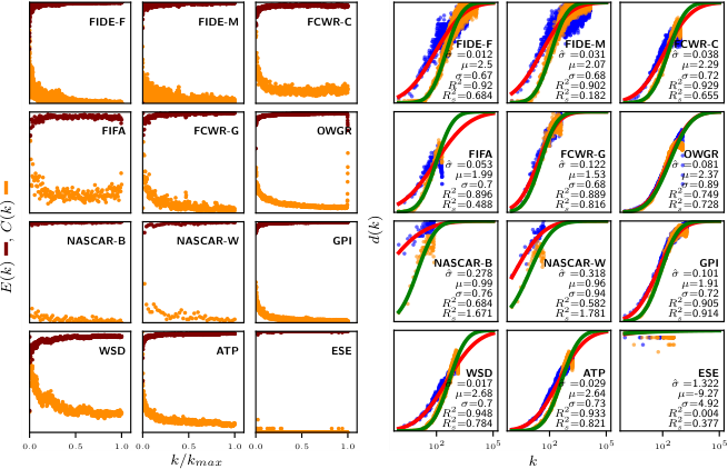
In Fig. 6 (left) the rank entropy for the twelve systems is given. We observe that in most games rank entropy is close to 1, which indicates that in these systems, predictability is low and the rank occupation is not stable, i.e., it is chaotic. It is to be noted that, in contrast to and , rank entropy shows that intermediate ranks have also a large amount of disorder. Still, lower ranks are slightly more predictable. In other words, it is easier (but still very limited) to predict who will be the first in a ranking (usually the safest bet would be that there would be no change) than to predict who would be in rank 100.
Following [20], we can define rank complexity as [9]:
| (9) |
This represents a balance between “order” () and “disorder” (), since is maximal (one) when and minimal (zero) when the entropy is at one of its extremes (zero or one). It has been argued that “critical” phenomena occur near a phase transition between order and chaos, and this coincides precisely with [15]. It can be said that measures a “balance” between order and chaos.
In Fig. 6 (left) the graphs for , show that the rank complexity is maximum when . It is clear that for FIDE, OWGR, FIFA, FCWR-G, WSD and ATP, is large for low , and has a relative stability, which is related to the small values of and for these ranks. In the other systems, complexity is small In particular, it will be seen that ESE shows for all ranks the minimum values of and the maximum values of . This, together with what was obtained for and , indicates that system ESE is chaotic at the scale observed, there is no way to characterize it. It might also be because of lack of data, and more frequent rankings would yield more meaningful results.
4 Random walk model
To reproduce the generic behavior of complex systems, the random walk model was introduced in Ref. [22]. In [7] it was shown that the hierarchical structure of systems could be related to the presence of random walks built with stochastic steps that follow a normal distribution. Consider the map
| (10) |
where represents the random number following Gaussian distributions with null average and standard deviation . Notice that the standard deviation in our model is proportional to the rank. This implies that elements with low ranks vary less in time than the elements with large ranks. must be then unfold so that at time we obtain all integers , albeit reordered. See [22] for more details.
The results are shown in Fig. 6 (right), where rank diversity for the twelve sports is compared with the one obtained using the random walk model. The blue points correspond to the data and the orange ones to the random model. The red curve is the sigmoid fitting the real data, while the green curve is the sigmoid that approximates the model data, recall eq. (6). One can see that the curves follow the data except for FIFA. This might be due to the fact that FIFA is the most “closed” system, i.e., few new elements enter or exit the ranking throughout time. It is to be noted that for the lowest ranks, the real data is always larger than the model one.
5 Discussion
By analyzing the rank dynamics of different sports, we found a common pattern: the top ranked players or teams tend to change their rank slower than the rest. This universal feature is independent of the nature of the sport, scoring systems, and ranking criteria. It is clear that rank changes in each sport will have different explanations. Still, the probability of change follows a common pattern. Exploring the rank diversity, closure, change probability, rank entropy, and rank complexity for different sports, we can find similarities among them and also measure how “fast” ranks change depending on the sport. This does not give us a strong predictive power, but allows us to infer how fast changes occur in different sports, and also how predictable outcomes in each competition are.
It is clear that sports with higher values of rank diversity and rank entropy imply that the ranks change faster. Prediction is limited, because it is not so probable that the previous top players and teams will remain at the top. This could be because chance is relatively more determinant than talent in the outcomes in those sports, but also could be because those sports are more competitive. Further work is needed to distinguish whether the shape of the rank diversity curves can be used as a proxy for the “randomness” or “competitiveness” of each sport [4, 13]. In this direction, it would also be interesting to analyze how “talent” and “luck” contribute to success in different sports [31, 25, 26, 17]. The “Science of Success” [2] is still at an early stage, and it could benefit and be benefited from statistical studies of performance and success in sports.
Acknowledgments
This work was supported by CONACyT under Grant CB-285754; and UNAM-PAPIIT under Grants IG101421, IN107919, and IV100120.
References
References
- [1] Atp world tour, http://www.atpworldtour.com/. Último acceso 10 de Enero de 2018.
- [2] Barabási, A. L. and Musciotto, F., Science of success: An introduction, in Computational Social Science and Complex Systems, eds. Kertész, J., Mantegna, R., and Miccichè, S. (IOS Press, 2019), pp. 57–72.
- [3] Batty, M., Rank clocks, Nature 444 (2006) 592–596.
- [4] Ben-Naim, E., Vazquez, F., and Redner, S., Parity and predictability of competitions, Journal of Quantitative Analysis in Sports 2 (2006).
- [5] Blumm, N., Ghoshal, G., Forró, Z., Schich, M., Bianconi, G., Bouchaud, J.-P., and Barabási, A.-L., Dynamics of ranking processes in complex systems, Physical review letters 109 (2012) 128701.
- [6] Clauset, A., Shalizi, C. R., and Newman, M. E., Power-law distributions in empirical data, SIAM review 51 (2009) 661–703.
- [7] Cocho, G., Flores, J., Gershenson, C., Pineda, C., and Sánchez, S., Rank diversity of languages: generic behavior in computational linguistics, PloS one 10 (2015) e0121898.
- [8] Football club world ranking, http://www.clubworldranking.com/ranking-clubs.aspx. Último acceso 10 de Enero de 2018.
- [9] Fernández, N., Maldonado, C., and Gershenson, C., Information measures of complexity, emergence, self-organization, homeostasis, and autopoiesis, in Guided self-organization: Inception (Springer, 2014), pp. 19–51.
- [10] Ferrer i Cancho, R. and Solé, R. V., Zipf’s law and random texts, Advances in Complex Systems 5 (2002) 1–6.
- [11] World chess federation, http://ratings.fide.com/. Último acceso 10 de Enero de 2018.
- [12] Fédération internationale de football association, http://www.fifa.com/. Accessed 6 April 2016.
- [13] Gabel, A. and Redner, S., Random walk picture of basketball scoring, Journal of Quantitative Analysis in Sports 8 (2012).
- [14] Gerlach, M. and Altmann, E. G., Stochastic model for the vocabulary growth in natural languages, Physical Review X 3 (2013) 021006.
- [15] Gershenson, C. and Fernández, N., Complexity and information: Measuring emergence, self-organization, and homeostasis at multiple scales, Complexity 18 (2012) 29–44.
- [16] Official world golf ranking, http://www.owgr.com/. Último acceso 10 de Enero de 2018.
- [17] Janosov, M., Battiston, F., and Sinatra, R., Success and luck in creative careers, EPJ Data Science 9 (2020) 9.
- [18] Kolmogorov, A. N., Sulla determinazione empirica di una legge di distribuzione, Giornale dell’Istituto Italiano degli Attuari 4 (1933) 83–91.
- [19] Li, W., Miramontes, P., and Cocho, G., Fitting ranked linguistic data with two-parameter functions, Entropy 12 (2010) 1743–1764.
- [20] Lopez-Ruiz, R., Mancini, H. L., and Calbet, X., A statistical measure of complexity, Physics Letters A 209 (1995) 321–326.
- [21] Morales, J. A., Colman, E., Sánchez, S., Sánchez-Puig, F., Pineda, C., Iñiguez, G., Cocho, G., Flores, J., and Gershenson, C., Rank dynamics of word usage at multiple scales, Frontiers in Physics 6 (2018) 45.
- [22] Morales, J. A., Sánchez, S., Flores, J., Pineda, C., Gershenson, C., Cocho, G., Zizumbo, J., Rodríguez, R. F., and Iñiguez, G., Generic temporal features of performance rankings in sports and games, EPJ Data Science 5 (2016) 33.
- [23] National association for stock car auto racing, http://www.espn.com/racing/standings Último acceso 10 de Enero de 2018.
- [24] Pappalardo, L. and Cintia, P., Quantifying the relation between performance and success in soccer, Advances in Complex Systems 21 (2018) 1750014.
- [25] Pluchino, A., biondo, A. E., and rapisarda, A., Talent versus luck: The role of randomness in success and failure, Advances in Complex Systems 21 (2018) 1850014.
- [26] Pluchino, A., Burgio, G., Rapisarda, A., Biondo, A. E., Pulvirenti, A., Ferro, A., and Giorgino, T., Exploring the role of interdisciplinarity in physics: Success, talent and luck, PLOS ONE 14 (2019) e0218793–.
- [27] Global poker index, http://www.globalpokerindex.com/. Último acceso 10 de Enero de 2018.
- [28] Shannon, C. E., A mathematical theory of communication, Bell System Technical Journal 27 (1948) 379–423 and 623–656.
- [29] World snowboarding, http://www.worldsnowboarding.org/ Último acceso 3 de Abril de 2018.
- [30] Videogame earnings, https://www.esportsearnings.com/history Último acceso 10 de Enero de 2018.
- [31] Yucesoy, B. and Barabási, A.-L., Untangling performance from success, EPJ Data Science 5 (2016) 17.
- [32] Zipf, G. K., Selected studies of the principle of relative frequency in language (Harvard University Press, Cambridge, MA, USA, 1932).