Period Change Rates in Large Magellanic Cloud Cepheids Revisited2021Period Change Rates in Large Magellanic Cloud Cepheids Revisited–References
Abstract
The period-change rate (PCR) of pulsating variable stars is a useful probe of changes in their interior structure, and thus of their evolutionary stages. So far, the PCRs of Classical Cepheids in the Large Magellanic Cloud (LMC) have been explored in a limited sample of the total population of these variables. Here we use a template-based method to build observed minus computed () period diagrams, from which we can derive PCRs for these stars by taking advantage of the long time baseline afforded by the Digital Access to a Sky Century @ Harvard (DASCH) light curves, combined with additional data from the Optical Gravitational Lensing Experiment (OGLE), the MAssive Compact Halo Object (MACHO) project, Gaia’s Data Release 2, and in some cases the All-Sky Automated Survey (ASAS). From an initial sample of 2315 sources, our method provides an unprecedented sample of 1303 LMC Classical Cepheids with accurate PCRs, the largest for any single galaxy, including the Milky Way. The derived PCRs are largely compatible with theoretically expected values, as computed by our team using the Modules for Experiments in Stellar Astrophysics (MESA) code, as well as with similar previous computations available in the literature. Additionally, five long-period () sources display a cyclic behavior in their diagrams, which is clearly incompatible with evolutionary changes. Finally, on the basis of their large positive PCR values, two first-crossing Cepheid candidates are identified.
Keywords:
stars: variables: Cepheids – stars: evolution – methods: data analysis – Magellanic Clouds1 Introduction
Classical or Type I Cepheids (hereafter Cepheids) are pulsating stars named after Cepheid, one of the first variable stars of this kind to be discovered (the first one actually being Aquilae; Catelan & Smith 2015, Catelan & Smith 2015). Owing to their period-luminosity relationship (Leavitt & Pickering 1912, also known as the Leavitt Law;) and intrinsic brightness, Cepheids play a key role in constraining the Hubble constant by working as standard candles (e.g., Freedman et al. 2001; Breuval et al. 2020; Riess et al. 2021, and references therein).
As they are intermediate-mass stars, their evolution is relatively fast and their ages are on the order of and yr for the longest-period (also the most massive and most luminous) and shortest-period (the least massive and least luminous) Cepheids, respectively. Their pulsations are excited by the and mechanisms, with the zone where helium goes from singly to doubly ionized being the most important for driving pulsations (see, e.g., Catelan & Smith 2015, and references therein).
Stellar evolution theory predicts three different stages where these stars become unstable to radial pulsations as they cross the instability strip in the Hertzsprung-Russell diagram (HRD): once during hydrogen shell burning and twice during core helium burning (Turner et al. 2006, e.g.,). According to the Stefan-Boltzmann law, a change in effective temperature at approximately constant luminosity implies a change in radius. Moreover, as the period-mean density relation (Ritter 1879, also known as Ritter’s relation;) is valid within the instability strip, changes in radius result in changes in period. Such period changes have been previously detected by numerous authors, and they seem to be more stable in Cepheids pulsating in the fundamental mode (Poleski 2008).
Period changes are useful for probing stellar evolution. Examples in the literature include, among many others, Pietrukowicz 2001, Turner et al. 2006, and Karczmarek et al. 2011 for Cepheids, and Le Borgne et al. 2007, Silva Aguirre et al. 2008, and Jurcsik et al. 2012 for RR Lyrae stars. Since theory predicts that the timescales for these evolutionary changes, , fall in the range yr (Poleski 2008, e.g.,), observations covering several decades are required to compute the associated period change rates (PCRs). A common technique that is used to conduct these measurements involves the so-called observed minus computed (O-C) diagrams (see Zhou 1999; Sterken 2005, for reviews and additional references). In this sense, the data for Cepheids in the Large Magellanic Cloud (LMC) that has been made available by the Digital Access to a Sky Century @ Harvard project (Grindlay et al. 2012, DASCH;) are suitable for the computation of PCRs, as they cover approximately a century. Modern CCD photometric surveys extend the baseline provided by DASCH even further, allowing the determination of more accurate PCRs than using DASCH alone.
Our goal in this paper is to calculate PCRs for LMC Classical Cepheids pulsating in the fundamental mode, using both DASCH data and more recent datasets from the literature. This also allows us to revisit previously published PCR values calculated for smaller Cepheid samples (Pietrukowicz 2001; Karczmarek et al. 2011), and to compare the measured values with those computed on the basis of state-of-the-art theoretical Cepheid models (e.g., Turner et al. 2006, Espinoza et al. 2021, in preparation).
2 Data
DASCH data play a crucial role in our computation of PCRs due to the time coverage of the observations included therein. We specifically make use of DASCH DR6 and, in order to further extend the time baseline coverage, data from other optical surveys were included, favoring observations obtained in the bands closest to that of the DASCH photometry (Tang et al. 2013, roughly Johnson ;). The surveys used to extend the time baseline are the MAssive Compact Halo Object Survey (Alcock et al. 2000, MACHO;), the Optical Gravitational Lensing Experiment (Udalski et al. 2015, OGLE;), and Gaia’s Data Release 2 (Gaia Collaboration et al. 2018; Evans et al. 2018, DR2;). Additionally, the longest-period, brightest Cepheids were usually saturated in the OGLE and MACHO surveys, therefore the DASCH data was augmented by the OGLE Shallow survey (Ulaczyk et al. 2012) and, when possible, the All-Sky Automated Survey (Pojmanski 2002, ASAS-3;), as replacements for the saturated OGLE photometry. A summary of the basic properties of these sources of data is provided in Table 1.
| Data | Code | Band | Date | Reference |
| yr | ||||
| DASCH | 1A, 1B | Photographic | Tang et al. 2013 | |
| MACHO | 2 | MACHO | Alcock et al. 2000 | |
| OGLE-III | 3 | Johnson | Soszynski et al. 2008 | |
| ASAS-3 | 4 | Johnson | Pojmanski 2002 | |
| OGLE Shallow | 5 | Johnson | Ulaczyk et al. 2012 | |
| OGLE-IV | 6 | Johnson | Udalski et al. 2015 | |
| Gaia DR2 | 7 | Gaia BP | Gaia Collaboration et al. 2018 |
3 Method
3.1 Source Selection
By using the OGLE Collection of Variable Stars (Soszyński et al. 2015, OCVS;), 2315 Cepheids pulsating in their fundamental mode were selected and their periods retrieved. Owing to the characteristics of the data in DASCH, the sample was split: While brighter and longer period sources often have clear and well-sampled light curves, fainter and shorter period sources tend to have incomplete phase coverage and show problems (such as blending) more frequently. Therefore, two subsets of data were utilized: 242 sources with OGLE and 2073 fainter sources.
As mentioned in Section 2, long-period sources () were saturated in OGLE and therefore they would not have measured magnitudes in the OCVS, although their periods are available. As a result, they were missing from our initial sample and had to be added manually. This added 5 sources to our sample.
Counterparts in MACHO (and ASAS, when necessary) were found by using the crossmatch tool provided with topcat (Taylor 2005) and a search radius. In the DASCH case, the sources’ respective OGLE IDs can be searched using DASCH’s light curve generator tool. Note that sometimes the latter procedure leads to multiple matches, in which case the closest and most complete matching source (i.e., the one with the higher number of observations) was selected.
3.2 Available Calibrations of the DASCH Survey
DASCH offers several photometric calibration options, from which only two were selected for this work. Analysis of light curves based on the different calibrations showed that generally the AAVSO Photometric All-Sky Survey (Henden et al. 2012, APASS;) calibration provides a good match with the unfiltered photographic plate blue, but it is limited to an APASS magnitude range between 9 and 15 mag. For fainter sources, the Guide Star Catalog 2.3.2 (Lasker et al. 2008, GSC2.3.2;) calibration is superior, in terms of quantity of data recovered from the photographic plates and phase coverage of the light curves.
Note that there are some sources near the limit of the APASS magnitude range which had data available under both calibrations, and so we had to decide which one to use for the final solution. The selection was based on the number of available points, coverage of the phase-folded light curve, and light curve scatter, the latter two steps done by visual inspection.
3.3 Data Preparation
Our method used for the calculation of the PCR values (see Section 3.4) implicitly assumes that the light curves have the same general properties. As this is not strictly true between the different surveys, we standardize the different data sets according to a few rules.
First, the time system of (modified Heliocentric Julian Date) used by the OGLE survey was adopted for all sources of data. Therefore, conversions were done when necessary, with the only exception of Gaia DR2 data, as its modified Barycentric Julian Date (BJD) system was not converted into HJD and instead only changed to . The reason for this is the relatively small expected difference of a few seconds (Seidelmann & Fukushima 1992, e.g.,) between HJD and Gaia BJD times of observations, which is irrelevant given the much longer pulsation periods of Cepheids.
In addition, in order to properly combine different data sets, a common zero-point and amplitude had to be enforced. This was done by subtracting the median magnitude from each data set and by scaling the magnitudes from each survey so they would have a common standard deviation, set to . This value is arbitrary, and was chosen purely because it allows us to recover approximately the amplitudes of large-amplitude Cepheids in the -band. However, due to the specifics of our method implementation, the choice of has no effect on the final derived period-change rates (as verified on a few variables by varying it in the range ). The method involving standard deviation was chosen over light curve normalization by amplitude due to the presence of outliers, especially in the case of DASCH light curves.
3.4 The Adopted O-C Method
The points in the diagram are derived from the timing differences between observed times of a specific point in the light curve, usually the maximum or minimum value, and the corresponding values computed (or expected) assuming a constant period. In this work, following Hertzsprung 1919, we use the entire light curve morphology to compute these differences. A light-curve template is constructed through a truncated Fourier series (TFS) as follows:
| (1) | |||||
| (2) |
where are the magnitudes of a section of the light curves used for the construction of the template, are the modified HJD times, is the OGLE period, is the number of terms in the series, and , , and are the parameters to be computed. This was done by using an ordinary least squares regression. We have conducted tests to determine the order of the TFS most appropriate to represent the Cepheid light curves. Visual inspection revealed that in most cases, is needed to properly represent the light curve (especially near the often rather steep rising branch).
The templates are constructed by using OGLE-IV data. When no OGLE-IV data are available, OGLE-III is used instead. To compare with the template light curve, data were split into bins of width 350 days, except for the DASCH data which, due to the higher scatter of the photographic light curves, generally require more data points, and hence wider bins, to measure values accurately. Therefore, in the latter case we applied bin widths of 1400 days.
The values were determined for all bins containing more than 10 points by minimizing the scatter between the template and the data in each of the bins. In practice, the data within each of the bins was folded with the adopted period, and the residuals minimized with a non-linear least-squares method, where the only variable is a shift applied to the times of the light-curve points. We estimated the values sequentially, starting with the most recent data and proceeding backwards in time, always using the last value estimated as the starting point in the non-linear optimization of the preceding (in time) bin.
We have also determined the uncertainty of each of the measured values using a bootstrapping method. We draw 100 new random data sets from the light curves within each of the data bins, for a number of points equal to the total within the respective bin, with replacement. The values of these bootstrapped samples were also determined, and their scatter with respect to the original value determined for each bin was adopted as the estimate of their uncertainties.
| Source | (J2000) | (J2000) | Data | Fourier Terms | Template | |||
|---|---|---|---|---|---|---|---|---|
| (deg) | (deg) | (d) | (d Myr-1) | (d Myr-1) | ||||
| 0005 | 68.881335 | -69.734944 | 5.6119491 | -3.2 | 1.3 | 1B, 3, 6, 7 | 10 | 6 |
| 0017 | 69.736785 | -69.688417 | 3.6772904 | -1.6 | 0.4 | 1B, 3, 6, 7 | 6 | 3, 7 |
| 0018 | 69.745755 | -68.956889 | 4.0478369 | 0.0 | 0.7 | 1B, 3, 6, 7 | 6 | 6 |
| 0021 | 69.879090 | -69.261833 | 5.4579579 | 5.3 | 1.5 | 1A, 3, 6, 7 | 10 | 6 |
| 0025 | 70.226535 | -69.115083 | 3.7334902 | 0.3 | 0.7 | 1B, 3, 6, 7 | 10 | 6 |
| 0027 | 70.331160 | -67.335583 | 3.5229124 | -1.9 | 0.3 | 1B, 3, 6, 7 | 10 | 6 |
| 0033 | 70.491375 | -69.433556 | 7.1807603 | 7.4 | 1.3 | 1A, 3, 6, 7 | 10 | 6 |
| 0034 | 70.507965 | -70.646944 | 11.2552749 | 68.4 | 9.1 | 1A, 3, 6, 7 | 8 | 6 |
| 0035 | 70.526295 | -67.969889 | 6.9435423 | 3.4 | 1.8 | 1A, 3, 6, 7 | 8 | 6 |
| 0039 | 70.658370 | -68.516472 | 3.1477882 | -0.1 | 0.6 | 1B, 3, 6 | 6 | 6, 7 |
Having computed the values, it is straightforward to build the diagrams. In these, the -axis corresponds to a representative time for each bin (mean of the bin edges), while the -axis is the found value. Assuming that the change in period is linear, we can expect a parabola in the diagram. The quadratic coefficient of this parabola is then related to the PCR (Sterken 2005, e.g.,) according to the following equation:
| (3) |
with the epoch and the average period. For the latter, we have used the periods exactly as given in the OCVS, as the absolute period change values are small in the case of Cepheids. Also, while the exact period value does change the appearance of the diagrams, it has a negligible effect on the measured period-change rates – i.e., on the order of seconds per year, as shown by observations and theoretical models alike (Turner et al. 2006). Therefore, in our computations we adopt .
To find the quadratic trend in the data and relate it to equation 3, a least-squares method which includes the uncertainties from each value as weights was used. This first result was taken as the starting point for the Markov chain Monte Carlo (MCMC) modeling. We used the emcee package (Foreman-Mackey et al. 2013), which implements an affine invariant ensemble method for the calculation of the posterior distribution of parameters. The logarithmic likelihood was adopted as follows:
| (4) | |||||
| (5) |
where is the equation that describes the quadratic model, are the coefficients of the quadratic polynomial fit, is the logarithmic likelihood, represents each of the bins of the diagram, are the values, and the uncertainties (standard deviations from the bootstrap). In this work, the EMCEE code was run using 32 walkers for 10000 steps, of which 5000 is the burn-in period, and a thinning factor of 15. For each of the parameters, the means and standard deviations of their marginalized posterior distributions are adopted as their final estimated values and uncertainties, respectively.
At this point, some difficulties were found and specific corrections were applied, as follows:
- i.
Due to the periodicity of the TFS and lack of data in some epochs, a shift in some values equal to (with ) was found. To fix this issue, a visual inspection and the required displacement equal to were executed.
- ii.
Some variables have little or no published -band photometry in OGLE. In these cases, the light-curve templates were constructed using either Gaia, a combination of OGLE (when available) and Gaia, or MACHO light curves.
- iii.
Some variables lack sharp features in their light curves. This sometimes results in unrealistic template shapes, when prepared using the default 10 Fourier terms. For these, the number of terms were reduced upon visual inspection. The changes are specified on table 2.
- iv.
Some Gaia light curves have poor phase coverage, resulting in scaling and zero-point problems. These were manually scaled after visual inspection.
- v.
Some sources were blended or would not have a distinguishable light curve in the DASCH data. Most of these required data selection using the DASCH quality flags.
- vi.
For the second subset (dim sources), blending, inadequate phase coverage and noise made the data preparation fail frequently. Therefore, an additional requirement of having more than 200 data points in DASCH as well as a period longer than 3 days was imposed on this subset after visual inspection of the preliminary results. Additionally, the magnitude scaling was changed from an automatic process to a semi-automatic one, allowing us to modify slightly the initial amplitude and zero-points when necessary, for a better agreement between data from different surveys.
The final results were obtained after implementing these changes to the fitting process, when necessary.
4 Results
We have successfully measured period-change rates for 1303 variables out of our initial sample of 2315. These values, alongside other supporting information, are listed in Table 2.
Figure 1 presents examples of diagrams and folded light curves (both before and after correcting for our measured PCR) for stars with positive, negative, and very small (consistent with zero) period changes.
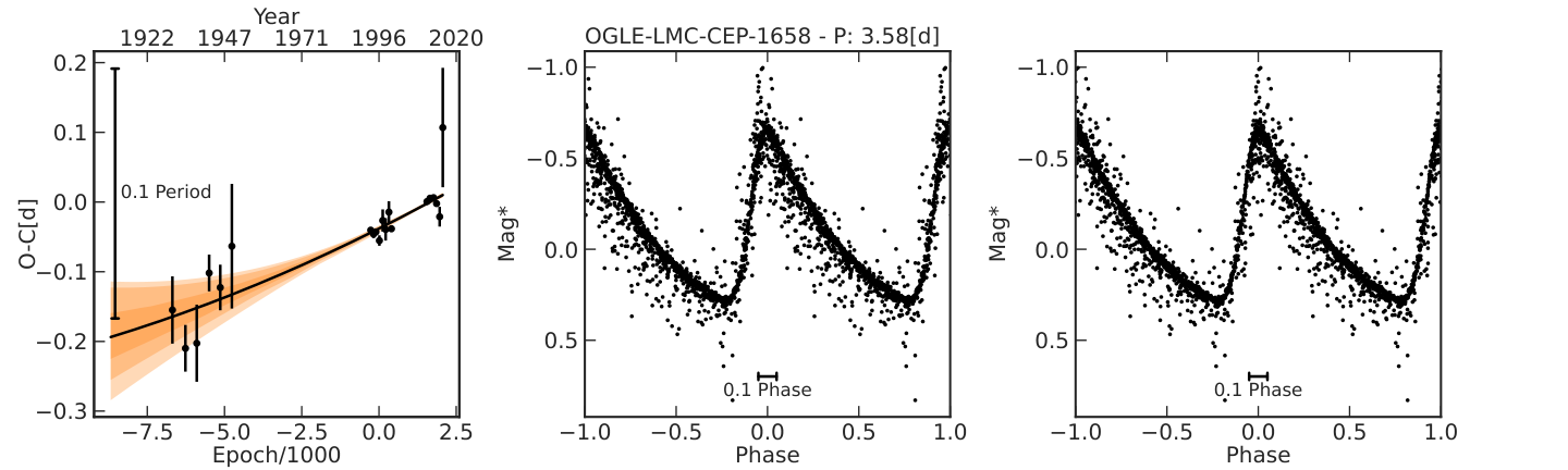
4.1 First Crossing Candidates
First-crossing Cepheids are very rare objects, as they are evolving very rapidly towards lower effective temperatures after crossing the Hertzsprung gap on the HRD. We detected two such candidates, namely OGLE-LMC-CEP-2840, with a period of and a PCR of , as well as OGLE-LMC-CEP-2132, which has a period of and a PCR of . In spite of their likely different metallicities, these results are comparable to what was found by Kovtyukh et al. 2019 for the Galactic Cepheid V1033 Cyg, which has a reported period of and a PCR of .
The diagrams and folded light curves for the new first-crossing candidates are shown in Figure 2. These sources were found upon visual inspection, as the algorithm could not account properly for the changes that occurred between the DASCH observations and more recent ones. For this reason, the diagrams were prepared, and the PCRs determined, without the DASCH data.
Nevertheless, in the case of OGLE-LMC-CEP-2132, the fit to the recent data allowed us to correct the DASCH observations for the effect of period changes and fold those, hence validating our approach. In the case of OGLE-LMC-CEP-2840, the scatter of the DASCH data prevents us from doing the same, unfortunately. As a further sanity check, we have also constructed the diagrams using the light curves obtained with the redder bands available for each data set (OGLE’s , Gaia’s RP, and MACHO’s ). The inferred PCR values, and for OGLE-LMC-CEP-2132 and OGLE-LMC-CEP-2840, respectively, are similar to those previously obtained for these stars, which provides further support for our analysis technique.
These variables are interesting targets for spectroscopic studies, as first-crossing Cepheids are expected to have surface abundances unaffected by the first dredge-up on the red giant branch (Kovtyukh et al. 2019), as they have not yet reached this phase in their evolution. In particular, Cepheids with lithium overabundances are thought to be in their first crossing (e.g., Luck et al. 2001; Kovtyukh et al. 2019; Catanzaro et al. 2020; Ripepi et al. 2021, and references therein), and thus a determination of the Li abundances in our two candidates would be of particular interest.
4.2 Comparison with Theoretical Models and Galactic Cepheids from Turner et al. (2006)
Turner et al. 2006 presented a detailed comparison between PCRs measured for Galactic Cepheids and the values expected from models. We present the dependence of the measured PCRs on the pulsation periods in Figure 3, following the example of (Turner et al. 2006, their Fig. 2). Although not all values fall within the expected areas for crossings according to Turner et al. 2006, we found 571 and 700 PCRs consistent with Cepheids on their second and third instability strip crossing according to their negative or positive PCR values, respectively. This implies an approximate ratio of between the number of sources with d in the second and third crossings. The remaining Cepheids include 30 sources that are consistent with no period changes plus two first-crossing candidates with large PCRs (Sect. 4.1).
In order to carry out a more systematic comparison with model predictions, we computed evolutionary models both with and without rotation for Classical Cepheids, using the Modules for Experiments in Stellar Astrophysics (MESA) code (Paxton et al. 2011). The pulsation analysis of the thus computed models was carried out using the Radial Stellar Pulsation (RSP) module, which is also integrated into MESA (Paxton et al. 2019). A full description of these calculations is beyond the scope of this paper, and will be provided in Espinoza-Arancibia et al. (2021, in preparation).
In Figure 3 we show the results of our calculations in the vs. plane, for a grid of Cepheid models of metallicity and initial masses between and , uniformly spaced in mass with a resolution of . Initial rotation was assumed to be solid body-like and values were taken in steps of within the range , where and are the angular velocity and its critical value, respectively. The loci occupied by these models is schematically indicated as shaded areas, whereas the lines represent the results from Turner et al. 2006. This figure shows that the predictions of these two sets of models are largely consistent (see Espinoza-Arancibia et al. 2021 for more details).
Note that there is also a good general agreement between the measured PCRs and their expected values from the models. This is observed over the full period range covered by the Cepheids in our sample, although our adopted low-mass limit does not allow us to draw strong conclusions regarding the behavior of the shortest-period Cepheids, as those are also the ones with the lowest masses. Similarly to Turner et al. 2006, who only detected one first-crossing candidate in their sample, we confirm that such stars are indeed rare, with only two candidates being present among 1303 stars (see Sect. 4.1).
4.3 Comparison with OGLE LMC Cepheids from Poleski (2008)
Poleski 2008 also carried out PCR measurements for LMC Cepheids, using data from the OGLE and MACHO projects, and compared his empirical results to the same Turner et al. 2006 models that were discussed in the previous subsection (see his Fig. 3). While many of his Cepheids do indeed fall within the expected region of the vs. plane according to both the Turner et al. 2006 and our models, the majority are placed outside it. In fact, there is even a large number of Cepheids in Poleski 2008 study whose position in this diagram would suggest that they are actually in their first crossing of the instability strip. Those results are in contrast with both our findings and those of Turner et al. 2006. Note that there are no tables with PCRs computed in Poleski 2008, and therefore our analysis is qualitative.
It is important to note that, while Poleski 2008 also used Fourier methods to compute period changes, a key difference lies in the amount of data, and the corresponding time coverage, upon which his measurements are based: Poleski 2008 was limited to MACHO, OGLE-II and OGLE-III data, and the relatively short implied time-span, of roughly 15 yr (compared with a typical 100 yr, in the case of our study), makes it difficult to properly measure the small PCRs of classical Cepheids. In addition, Poleski 2008 carried out individual measurements over timescales of days, as opposed to the timescales of years used in our analysis. This implies, as indeed pointed out in this study, that his results are much more sensitive to random period fluctuations. In particular, his short-period sources () seem to be dominated by these, tending to fall outside the areas expected for the different crossings as can be seen in his Figure 3. While we do not find the exact same behavior (as can be seen in our Figure 3, which is equivalent to his Figure 3), we do find an increase in the uncertainties in our PCR measurements for Cepheids in the short-period regime. Similarly, visual inspection of the second subset of sources (i.e., those with ) revealed that many of the sources in the short-period end of our sample () showed an erratic behavior that cannot be adequately described by a parabola, contrary to theoretical expectations. This is related to short-period Cepheids being intrinsically fainter and having bigger uncertainties, as can be seen from the typical value of magnitude uncertainty (acquired from the estimated error of the locally corrected magnitude measurement in the DASCH data), which is and increases to for typical Cepheids of magnitude and fainter than in the -band, respectively (or, equivalently, ). While this behavior is more common on these short-period Cepheids, there are some Cepheids with longer periods that show a similar behavior. As an example, the individual values obtained for the Cepheid OGLE-LMC-CEP-0975, with a period of , have for the most part very small uncertainties, as can be seen in the middle panel of Figure 4. However, it is also possible to notice in the same panel that there is no clear quadratic trend in the diagram. The other two panels in Figure 4 show additional examples, but in the short-period regime.
As mentioned earlier, it is possible that these fluctuations are related to the timescales used. In our analysis, they become more noticeable when the period changes themselves become smaller, which is reflected in the diagrams as values smaller than a day. This could mean that the PCR fluctuations become relevant when they are of similar order as the period changes, which would explain their larger incidence as one approaches the short-period regime. On the other hand, this explanation would not be adequate in the case of long-period Cepheids with erratic behavior, such as OGLE-LMC-CEP-0975. For further discussion about the possible origins of these fluctuations in Cepheids, the reader is referred to Szabados 1983 and Neilson & Ignace 2014.
4.4 Previously Computed Values for PCRs in the LMC
Both Pietrukowicz 2001 and Karczmarek et al. 2011 computed PCRs for Cepheids in the LMC as well. While Karczmarek et al. 2011 only used ASAS data, Pietrukowicz 2001 employed a data set with a time baseline similar to the one employed in this work, by using the Harvard (Payne-Gaposchkin 1971, as collected by), ASAS, and OGLE data. The results for sources in common between each of those two studies and ours are shown in Figure 5.
Close examination of this plot reveals that there is a larger fraction of sources with similar PCRs as measured by us in Pietrukowicz 2001 than in Karczmarek et al. 2011. Indeed, the latter’s measurements tend to differ from ours by an amount that can reach several orders of magnitude, even in the cases where the sign of their measured period variations is the same as found by us.
A possible explanation for the differences between our results and those by Karczmarek et al. 2011 could be related to the more limited dataset used by these authors, both in comparison with our work and Pietrukowicz 2001, and also their focus on variations that occur on shorter timescales. This could lead to their results being dominated by high-frequency noise, as in Poleski 2008. This idea is indeed supported by Figure 8 in Karczmarek et al. 2011, where a comparison with Poleski 2008 is shown.
To close, we note that the differences between our results and those by Pietrukowicz 2001 tend to increase with decreasing (absolute) values. We have verified that this behavior is primarily caused by the shorter-period Cepheids (our second data subset). This is expected, as data availability and quality in DASCH decreases with decreasing magnitude (period).
4.5 O-C Diagram Results for Long-Period Cepheids
Examples of results for bright Cepheids () are shown in Figure 6. Some properties of these sources are provided in Table 3, where no PCRs are reported, since the computed quadratic trends are not representative of their complex diagrams.
Analysis of these plots suggests that, in addition to a possible quadratic component, which could plausibly be related to the long-term, secular evolution of the star, an additional, cyclic component may also be present, which may perhaps be described using a quasi-sinusoidal term (see Sterken 2005, his Sect. 4.2). A similar phenomenon is apparent in the diagrams of the two Galactic Cepheids with the longest known periods, namely V1496 Aql, with d, and S Vul, with d (Berdnikov et al. 2004). The actual mechanism that is responsible for these variations is, however, unclear. A possible explanation might include the presence of one or more companions, which would impact the diagram of the Cepheid by means of the light-travel time effect, as indeed seen in RR Lyrae binaries (Hajdu et al. 2015; Hajdu et al. 2021, e.g.,). However, both the amplitude of the variations and the fact that the latter are seen in all our long-period sources, as well as in V1496 Aql and S Vul, make binarity an unlikely general explanation of the phenomenon.


5 Summary and Conclusions
| Source | Data | Fourier | Template | |
|---|---|---|---|---|
| (d) | ||||
| 0619 | 133.78 | 1A, 4, 5, 7 | 10 | 5 |
| 0992 | 52.87 | 1A, 2, 4, 5, 7 | 10 | 5 |
| 1591 | 118.62 | 1A, 2, 4, 5, 7 | 10 | 5 |
| 4628 | 99.2 | 1A, 4, 7 | 6 | 4 |
| 4689 | 78.51 | 1A, 4, 7 | 6 | 4 |
Using data from the literature, spanning over 100 years in some cases, we have employed the diagram technique to derive PCRs for an unprecedented sample of 1303 Classical Cepheids in the LMC covering a broad range of periods. Our results were compared with previous results from the literature and with a new set of evolutionary and pulsation models of Classical Cepheids for an LMC-like metallicity and with rotation, computed with MESA. The latter will be presented in more detail in Espinoza-Arancibia et al. (2021, in preparation). Our main conclusions can be summarized as follows.
Our model predictions are substantially in agreement with those previously presented by Turner et al. 2006, over a similar mass range. Both model sets also seem to correctly describe the overall PCR behavior in Classical Cepheids, as brought about by secular stellar evolution. This allowed us to identify two new first-crossing candidates, for which we suggest spectroscopic follow-up, in order to confirm the presence of typical spectral signatures seen in first-crossing Cepheids, particularly Li enhancement. The majority of the remaining sources have PCR values that are consistent with these Cepheids being in the second or third crossing of the instability strip, as expected.
Comparison with previous PCR measurements show reasonable agreement with Pietrukowicz 2001, but significant differences with respect to Karczmarek et al. 2011 are present. Neither use an approach and the more limited dataset used by the latter authors (a baseline of only 10 yr), is likely the main reason of the noted differences, given that both a much longer time span was considered in both Pietrukowicz 2001 and our study. As in Poleski 2008, the finer time resolution adopted by Karczmarek et al. 2011 in their study could also make their analysis sensitive to erratic period changes that take place at much shorter timescales than probed by us, since we often binned together data spanning multiple years, in order to increase the statistical significance of our results and to more reliably analyze long-term trends.
As a rule, the diagrams that we obtained for long-period Cepheids, i.e., Cepheids with periods longer than about 50 d, do not show the typical quadratic behavior that would have been expected in the case of linear period changes, but rather fluctuations, which sometimes can be very substantial, superimposed on a global long-term trend. Following Sterken 2005, we suggest that this behavior might be successfully described in terms of a combination of two terms, namely a quadratic one, reflecting the secular evolution of the physical properties of the star, and a cyclical, quasi-sinusoidal one, whose physical origin is still unclear. We speculate that the latter could in principle be caused by the presence of one or more companions, but the fact that a similar behavior is seen in all long-period Cepheids, and often with very high amplitudes in their corresponding diagrams, renders this an unlikely general explanation, as does the fact that the implied minimum masses of the companion would be in excess of in all cases. This approximation for the masses was computed by using the binary mass function and the eye-approximate period (around 50 yr) and semi-major axis (about 2000 AU) of an edge-on view of the assumed binary orbit.
Acknowledgements
Support for this project is provided by ANID’s Millennium Science Initiative through grant ICN12_12009, awarded to the Millennium Institute of Astrophysics (MAS); by ANID’s Basal projects AFB-170002 and FB210003; and by FONDECYT grant #1171273. The research leading to these results has received funding from the European Research Council (ERC) under the European Union’s Horizon 2020 research and innovation programme (grant agreement No 695099). CC, COH, and AVN acknowledge support from the National Agency for Research and Development (ANID), Scholarship Program Doctorado Nacional, grant numbers 2021 – 21212083, 2018 – 21180315, and 2020 – 21201226, respectively. The DASCH project at Harvard was partially supported by the NSF grants AST-0407380, AST-0909073, and AST-1313370. We are grateful for the efforts of the DASCH project for making the present study possible.
Data Availability
The derived data generated in this article are available in its online supplementary material. This dataset was derived from sources in the public domain: the ASAS Catalogue of Variable Stars, the DASCH Lightcurve Access portal, the Gaia Archive, the OGLE Project and the MACHO Data Services .
References
- Alcock et al. (2000) Alcock C., et al., 2000, ApJ, 542, 281
- Berdnikov et al. (2004) Berdnikov L. N., Samus N. N., Antipin S. V., Ezhkova O. V., Pastukhova E. N., Turner D. G., 2004, PASP, 116, 536
- Breuval et al. (2020) Breuval L., et al., 2020, A&A, 643, A115
- Catanzaro et al. (2020) Catanzaro G., et al., 2020, A&A, 639, L4
- Catelan & Smith (2015) Catelan M., Smith H. A., 2015, Pulsating Stars. Wiley-VCH
- Evans et al. (2018) Evans D. W., et al., 2018, A&A, 616, A4
- Foreman-Mackey et al. (2013) Foreman-Mackey D., Hogg D. W., Lang D., Goodman J., 2013, PASP, 125, 306
- Freedman et al. (2001) Freedman W. L., et al., 2001, ApJ, 553, 47
- Gaia Collaboration et al. (2018) Gaia Collaboration et al., 2018, A&A, 616, A1
- Grindlay et al. (2012) Grindlay J., Tang S., Los E., Servillat M., 2012, in Griffin E., Hanisch R., Seaman R., eds, IAU Symposium Vol. 285, New Horizons in Time Domain Astronomy. pp 29–34 (arXiv:1211.1051), doi:10.1017/S1743921312000166
- Hajdu et al. (2015) Hajdu G., Catelan M., Jurcsik J., Dekany I., Drake A. J., Marquette J. B., 2015, MNRAS, 449, L113
- Hajdu et al. (2021) Hajdu G., et al., 2021, ApJ, 915, 50
- Henden et al. (2012) Henden A. A., Smith T. C., Levine S. E., Terrell D., 2012, in American Astronomical Society Meeting Abstracts #220. p. 133.06
- Hertzsprung (1919) Hertzsprung E., 1919, Astronomische Nachrichten, 210, 17
- Jurcsik et al. (2012) Jurcsik J., et al., 2012, MNRAS, 419, 2173
- Karczmarek et al. (2011) Karczmarek P., Dziembowski W. A., Lenz P., Pietrukowicz P., Pojmański G., 2011, Acta Astron., 61, 303
- Kovtyukh et al. (2019) Kovtyukh V., et al., 2019, MNRAS, 488, 3211
- Lasker et al. (2008) Lasker B. M., et al., 2008, AJ, 136, 735
- Le Borgne et al. (2007) Le Borgne J. F., et al., 2007, A&A, 476, 307
- Leavitt & Pickering (1912) Leavitt H. S., Pickering E. C., 1912, Harvard College Observatory Circular, 173, 1
- Luck et al. (2001) Luck R. E., Kovtyukh V. V., Andrievsky S. M., 2001, A&A, 373, 589
- Neilson & Ignace (2014) Neilson H. R., Ignace R., 2014, A&A, 563, L4
- Paxton et al. (2011) Paxton B., Bildsten L., Dotter A., Herwig F., Lesaffre P., Timmes F., 2011, ApJS, 192, 3
- Paxton et al. (2019) Paxton B., et al., 2019, ApJS, 243, 10
- Payne-Gaposchkin (1971) Payne-Gaposchkin C. H., 1971, Smithsonian Contributions to Astrophysics, 13
- Pietrukowicz (2001) Pietrukowicz P., 2001, Acta Astron., 51, 247
- Pojmanski (2002) Pojmanski G., 2002, Acta Astron., 52, 397
- Poleski (2008) Poleski R., 2008, Acta Astron., 58, 313
- Riess et al. (2021) Riess A. G., Casertano S., Yuan W., Bowers J. B., Macri L., Zinn J. C., Scolnic D., 2021, ApJ, 908, L6
- Ripepi et al. (2021) Ripepi V., et al., 2021, A&A, 647, A111
- Ritter (1879) Ritter A., 1879, Annalen der Physik, 244, 157
- Seidelmann & Fukushima (1992) Seidelmann P. K., Fukushima T., 1992, A&A, 265, 833
- Silva Aguirre et al. (2008) Silva Aguirre V., Catelan M., Weiss A., Valcarce A. A. R., 2008, A&A, 489, 1201
- Soszynski et al. (2008) Soszynski I., et al., 2008, Acta Astron., 58, 163
- Soszyński et al. (2015) Soszyński I., et al., 2015, Acta Astron., 65, 297
- Sterken (2005) Sterken C., 2005, in Sterken C., ed., Astronomical Society of the Pacific Conference Series Vol. 335, The Light-Time Effect in Astrophysics: Causes and cures of the O-C diagram. p. 3
- Szabados (1983) Szabados L., 1983, Ap&SS, 96, 185
- Tang et al. (2013) Tang S., Grindlay J., Los E., Servillat M., 2013, PASP, 125, 857
- Taylor (2005) Taylor M. B., 2005, in Shopbell P., Britton M., Ebert R., eds, Astronomical Society of the Pacific Conference Series Vol. 347, Astronomical Data Analysis Software and Systems XIV. p. 29
- Turner et al. (2006) Turner D. G., Abdel-Sabour Abdel-Latif M., Berdnikov L. N., 2006, PASP, 118, 410
- Udalski et al. (2015) Udalski A., Szymański M. K., Szymański G., 2015, Acta Astron., 65, 1
- Ulaczyk et al. (2012) Ulaczyk K., et al., 2012, Acta Astron., 62, 247
- Zhou (1999) Zhou A., 1999, Publications of the Beijing Astronomical Observatory, 33, 17