Full-color three-loop three-point form factors in ${\cal N}=4$ SYM

Guanda Lin Email: linguandak@pku.edu.cn Affiliation: CAS Key Laboratory of Theoretical Physics, Institute of Theoretical Physics,
Chinese Academy of Sciences, Beijing 100190, China Affiliation: School of Physics, Peking University, Beijing 100871, China Gang Yang Email: yangg@itp.ac.cn Affiliation: CAS Key Laboratory of Theoretical Physics, Institute of Theoretical Physics,
Chinese Academy of Sciences, Beijing 100190, China Affiliation: School of Physical Sciences, University of Chinese Academy of Sciences, Beijing 100049, China Affiliation: School of Fundamental Physics and Mathematical Sciences, Hangzhou Institute for Advanced Study, UCAS, Hangzhou 310024, China Affiliation: International Centre for Theoretical Physics Asia-Pacific, Beijing/Hangzhou, China Affiliation: Peng Huanwu Center for Fundamental Theory, Xian 710127, China and Siyuan Zhang Email: zhangsiyuan@itp.ac.cn Affiliation: CAS Key Laboratory of Theoretical Physics, Institute of Theoretical Physics,
Chinese Academy of Sciences, Beijing 100190, China Affiliation: School of Physical Sciences, University of Chinese Academy of Sciences, Beijing 100049, China

Abstract

We present the detailed computation of full-color three-loop three-point form factors of both the stress-tensor supermultiplet and a length-three BPS operator in ${\cal N}=4$ SYM. The integrands are constructed based on the color-kinematics (CK) duality and generalized unitarity method. An interesting observation is that the CK-dual integrands contain a large number of free parameters. We discuss the origin of these free parameters in detail and check that they cancel in the simplified integrands. We further perform the numerical evaluation of the integrals at a special kinematics point using public packages FIESTA and pySecDec based on the sector-decomposition approach. We find that the numerical computation can be significantly simplified by expressing the integrals in terms of uniformly transcendental basis, although the final three-loop computations still require large computational resources. Having the full-color numerical results, we verify that the non-planar infrared divergences reproduce the non-dipole structures, which firstly appear at three loops. As for the finite remainder functions, we check that the numerical planar remainder for the stress-tensor supermultiplet is consistent with the known result of the bootstrap computation. We also obtain for the first time the numerical results of the three-loop non-planar remainder for the stress-tensor supermultiplet as well as the three-loop remainder for the length-three operator.

1 Introduction

Significant progress has been made in the last thirty years in our understanding of scattering amplitudes, in which the modern on-shell methods have played important roles, see e.g. Elvang:2013cua; Henn:2014yza for an introduction. Form factors, as quantities that encode the information of both on-shell asymptotic states and off-shell local operators, have also attracted increasing attentions in recent years. Specifically, an $n$ -point form factor can be defined as the matrix element between $n$ on-shell asymptotic states and a local gauge invariant operator $\mathcal{O}$ as

\mathcal{F}_{\mathcal{O}}(1,\ldots,n;q)\equiv\int d^{D}xe^{-iq\cdot x}\langle 1\ldots n|\mathcal{O}(x)|0\rangle=(2\pi)^{D}\delta^{(D)}\Big(q-\sum_{i=1}^{n}p_{i}\Big)\langle 1\ldots n|\mathcal{O}(0)|0\rangle\,.

(1)

Since form factors involve both on-shell states and local operators, they may be taken as a bridge between on-shell amplitudes and off-shell correlation functions, in particular, it is possible to apply powerful modern techniques originally designed for amplitudes to study them. Indeed, much advance has been made in the studies of form factors in ${\cal N}=4$ SYM, including the strong-coupling picture via AdS/CFT correspondence Alday:2007he; Maldacena:2010kp; Gao:2013dza, MHV structure and supersymmetric formalisms Brandhuber:2010ad; Bork:2010wf; Brandhuber:2011tv; Bork:2011cj, Grassmannian and polytope pictures Frassek:2015rka; Bork:2016hst; Bork:2016xfn; Bork:2017qyh; Bork:2014eqa, twistor formalism Koster:2016ebi; Koster:2016loo; Chicherin:2016qsf; Koster:2016fna, and the connected description of form factors He:2016dol; Brandhuber:2016xue; He:2016jdg. Generalized unitarity method has been applied to high-loop form factors of BPS operators Gehrmann:2011xn; Brandhuber:2012vm; Brandhuber:2014ica and non-protected operators Wilhelm:2014qua; Nandan:2014oga; Loebbert:2015ova; Brandhuber:2016fni; Loebbert:2016xkw; Caron-Huot:2016cwu. Bootstrap methods have also proved to be successful for form factors: the symbol bootstrap method has been applied to form factors at two loops Brandhuber:2012vm and recently at much higher loops in Dixon:2020bbt with the help of the form factor operator product expansion (OPE) Sever:2020jjx; Sever:2021nsq; besides, a new bootstrap strategy based on the master-integral ansatz has been developed to compute a two-loop four-point form factor in Guo:2021bym. See also some other studies in Henn:2011by; Bork:2012tt; Engelund:2012re; Johansson:2012zv; Huang:2016bmv; Ahmed:2016vgl; Bolshov:2018eos; Bianchi:2018peu; Bianchi:2018rrj. A recent introduction and review of form factors in ${\cal N}=4$ SYM can be found in Yang:2019vag.

In this paper, we study a special class of three-point form factors in ${\cal N}=4$ SYM at three loops with complete color dependence. We focus on the form factors of the BPS operators, $\operatorname{tr}(\phi^{2})$ and $\operatorname{tr}(\phi^{3})$ . Although we consider form factors in ${\cal N}=4$ SYM, they are closely related to Higgs amplitudes in QCD. In particular, scattering of Higgs and gluons can be understood as form factors of operators appearing in the Higgs effective theory, where Higgs-gluons interaction vertices are obtained by integrating out the heavy top quark loop Ellis:1975ap; Georgi:1977gs; Wilczek:1977zn; Shifman:1979eb. Many evidences from form factor results at two loops Gehrmann:2011aa; Brandhuber:2012vm; Brandhuber:2014ica; Loebbert:2015ova; Brandhuber:2016fni; Loebbert:2016xkw; Banerjee:2016kri; Brandhuber:2017bkg; Banerjee:2017faz; Jin:2018fak; Brandhuber:2018xzk; Brandhuber:2018kqb; Jin:2019ile; Jin:2019opr; Jin:2020pwh support the intriguing maximal transcendentality principle (MTP) Kotikov:2002ab; Kotikov:2004er which conjectures that $\mathcal{N}=4$ SYM captures the maximally transcendental part of QCD. The new results obtained in this paper are also expected to provide the maximally transcendental pieces of three-loop QCD results.

Our strategy for calculating these three-loop form factors, in particular to get the full-color integrands, is to apply the color-kinematics (CK) duality Bern:2008qj; Bern:2010ue. The CK duality implies a direct connection between the color and kinematics of gauge amplitudes or form factors, and thus provides a powerful practical tool to construct loop integrands. Together with the generalized unitarity method Bern:1994zx; Bern:1994cg; Britto:2004nc, many non-trivial high-loop constructions have been achieved with the help of CK duality, see e.g. high-loop amplitudes in SYM Carrasco:2011mn; Bern:2012uf; Bern:2013qca; Bern:2014sna; Johansson:2017bfl; Bern:2017ucb; Kalin:2018thp and pure YM Boels:2013bi; Bern:2013yya; Bern:2015ooa; Mogull:2015adi, and also form factors in ${\cal N}=4$ SYM Boels:2012ew; Yang:2016ear; Lin:2020dyj. Apart from its significance in gauge theories, the duality also make it possible to compute gravity amplitudes via the double-copy of gauge amplitudes, which has played an important role in studying the (super)gravity theories and their ultraviolet divergences, see e.g. Bern:2017ucb; Bern:2017yxu; Bern:2012gh; Bern:2012cd; Bern:2012uf; Bern:2010ue. See Bern:2019prr for an extensive review of the duality and its applications.

Although the CK duality has been understood at tree level BjerrumBohr:2009rd; Stieberger:2009hq; Feng:2010my, it is still a conjecture at loop level. Thus, it is important to explore more explicit constructions and see to what extent the duality applies. The CK-dual integrands constructed in this paper offer new non-trivial three-loop examples which suggest that the CK-duality structure should exist in more general situations. Interestingly, the new form factor integrands show a novel feature compared with the amplitude cases: the CK-dual solutions contain a large number of free parameters which originate from a new type of generalized gauge transformations induced by the insertion of operator in form factors. We would also like to stress the results take the “simplest” form, in the sense that they have the minimal power counting of loop momenta expected in $\mathcal{N}=4$ SYM and manifest all diagrammatic symmetries.

The form factors after integration are also expected to possess interesting structures. Starting from three loops, infrared (IR) divergences receive contributions beyond the dipole form Almelid:2015jia, which should be observed in our three-point form factors as well. To study these structures, we also compute the three-loop integrals using the numerical approach based on sector decomposition strategy Binoth:2000ps with pubic programs FIESTA Smirnov:2015mct and pySecDec Borowka:2017idc. To tackle the complicated three-loop non-planar integrals, an improved representation based on the $d\log$ -form integrals is also employed Arkani-Hamed:2014via; Bern:2014kca. Such $d\log$ integrals have simple pole structures and empirical observations show that it is much more efficient to evaluate them numerically than ordinary Feynman integrals. A similar observation was also made for the four-loop Sudakov form factor in Boels:2017ftb. We obtain the numerical results of full-color form factors for both $\operatorname{tr}(\phi^{2})$ and $\operatorname{tr}(\phi^{3})$ operators up to the $O(\epsilon^{0})$ order at a special phase space point. Our three-loop results consistently reproduce the IR structure with non-dipole corrections Almelid:2015jia and also verify the planar remainder of the operator $\operatorname{tr}(\phi^{2})$ obtained from the bootstrap method Dixon:2020bbt.

Finally, we mention that the integrands of the above three-loop form factors have been reported in the short letter Lin:2021kht, while in this paper we present more details, including the non-planar unitarity cuts and the parameter cancellation in the solution space, as well as new results on the integral simplification and evaluation. The organization of this paper is as follows. In Section 2, we provide a detailed description of our strategy for constructing integrands in the CK-dual representation. The three-loop integrands satisfying CK duality are discussed in Section 3, where the two-loop three-point form factor for $\operatorname{tr}(\phi^{2})$ is also revisited as a warm-up example. Section 3 also includes an analysis on the aforementioned parameters in the integrands, reflecting new features for form factors. Then we describe the method and results for simplifying and reorganizing the integrands in Section 4, so that the integrands are suitable for subsequent numerical evaluations. The numerical integration, IR subtraction and remainders are discussed in Section 5. Some details and data appearing in all these discussions are presented in Appendix A–D.

2 Strategy for loop-integrand construction

In this section, we describe the general strategy for constructing loop integrand by color-kinematics duality and unitarity cuts. First, we give a brief review of color-kinematics duality and describe how to use it to construct an ansatz for the loop integrand of form factors. Then we explain how to apply physical constraints to fix the ansatz, including diagrammatic symmetries and unitarity cuts, where a particular emphasis will be on the application of non-planar cuts. Readers are also referred to Bern:2012uf; Carrasco:2015iwa; Yang:2019vag for some further details of the strategy.

2.1 CK duality and the construction of ansatz

Color-kinematics duality refers to the statement that it is possible to rearrange the perturbative amplitudes in gauge theories, such that the Jacobi relations satisfied by color factors of cubic graphs also apply to the kinematics numerators of the same graphs Bern:2008qj; Bern:2010ue.

The simplest example to illustrate this duality should be the four-gluon tree amplitude. The CK-dual representation of this amplitude takes the following form:

\textbf{{A}}^{(0)}_{4}=\frac{C_{s}N_{s}}{s}+\frac{C_{t}N_{t}}{t}+\frac{C_{u}N_{u}}{u}\,,

(2)

where $C_{s,t,u}$ and $N_{s,t,u}$ are color factors and numerators of the $s$ -, $t$ - and $u$ -channel cubic graphs respectively:

\begin{aligned} \includegraphics[height]{figure/A4tree.eps}\end{aligned}.

(3)

The color factors are defined by attaching a structure constant $\tilde{f}^{abc}$ to each trivalent vertex, namely

C_{s}=\tilde{f}^{a_{1}a_{2}\rm{x}}\tilde{f}^{a_{3}a_{4}\rm{x}},\qquad C_{t}=\tilde{f}^{a_{4}a_{1}\rm{x}}\tilde{f}^{a_{2}a_{3}\rm{x}},\qquad C_{u}=\tilde{f}^{a_{3}a_{1}\rm{x}}\tilde{f}^{a_{4}a_{2}\rm{x}}\,,

(4)

where

\tilde{f}^{abc}=\operatorname{tr}(T^{a}T^{b}T^{c})-\operatorname{tr}(T^{a}T^{c}T^{b})\,,

(5)

and the color generators $T^{a}$ are normalized as $\operatorname{tr}(T^{a}T^{b})=\delta^{ab}$ . For concreteness, we will often consider the $\text{SU}(N_{c})$ gauge group in this paper.

As for the numerators, the requirement of color-kinematics duality means that the kinematics numerators satisfy the same algebraic relation as the color factors:

C_{s}=C_{t}+C_{u}\quad\Rightarrow\quad N_{s}=N_{t}+N_{u}\,.

(6)

It is easy to obtain such a numerator solution for the four-gluon amplitude:

		$\displaystyle N_{s}=\left(\mathcal{E}_{12}{\bf p}_{12}^{\mu}+2\mathcal{P}_{21}\varepsilon_{2}^{\mu}-2\mathcal{P}_{12}\varepsilon_{1}^{\mu}\right)\left(\mathcal{E}_{34}{\bf p}_{34,\mu}+2\mathcal{P}_{43}\varepsilon_{4,\mu}-2\mathcal{P}_{34}\varepsilon_{3,\mu}\right)+s_{12}\left(\mathcal{E}_{13}\mathcal{E}_{24}-\mathcal{E}_{14}\mathcal{E}_{23}\right),$
		$\displaystyle N_{t}=\left.N_{s}\right\|_{1\leftrightarrow 3},\qquad N_{u}=\left.N_{s}\right\|_{2\leftrightarrow 3},$		(7)

where $\mathcal{E}_{ij}=\varepsilon_{i}\cdot\varepsilon_{j}$ , $\mathcal{P}_{ij}=p_{i}\cdot\varepsilon_{j}$ , and ${\bf p}_{ij}=p_{i}-p_{j}$ , with $p_{i}$ and $\varepsilon_{i}$ the momentum and polarization vector of the $i$ -th particle. We also remark that the on-shell conditions for the four external legs are needed to show that (6) is indeed a CK-dual solution.

The highly non-trivial observation is that the color-kinematics duality can be generalized at loop level. For the form factors considered in this paper, the loop integrand in a representation satisfying CK duality can be expressed in the following form:

\textbf{{F}}^{(\ell)}_{\mathcal{O},n}=\sum_{\sigma}\sum_{\Gamma_{i}}\int\prod_{j=1}^{\ell}\frac{\mathrm{d}^{D}l_{j}}{(2\pi i)^{D}}\frac{1}{S_{i}}\sigma\cdot\frac{C_{i}{\tilde{N}}_{i}}{\prod_{\alpha_{i}}P^{2}_{\alpha_{i}}}\,,

(8)

where

1.

$\Gamma_{i}$ represent topological distinct trivalent graphs, with $i$ labelling of the graphs;
2.

$S_{i}$ are symmetry factors determined by the graph symmetry of the corresponding $\Gamma_{i}$ ;
3.

$P^{2}_{\alpha_{i}}$ are Feynman propagators corresponding to $\Gamma_{i}$ ;
4.

$C_{i}$ are color factors of diagram $\Gamma_{i}$ composed of the following two parts: each trivalent vertex contributes a structure constant $\tilde{f}^{abc}$ ; as for the operator vertex, the associated color factor is determined by the operator $\mathcal{O}$ ;
5.

The kinematics numerators are ${\tilde{N}}_{i}$ and can be factorized as ${\cal F}_{\mathcal{O},n}^{(0)}N_{i}$ , where the tree-level form factor ${\cal F}_{\mathcal{O},n}^{(0)}$ carries all helicity weights, and $N_{i}$ are functions of loop and external momenta, which will be the central object of the discussions below;
6.

The sum over $\sigma$ refers to summing all permutations of external legs, as well as possible inequivalent permutations of legs directly connected to the operator; and $\sigma$ acts on ${\tilde{N}}_{i},P^{2}_{\alpha_{i}}$ and $C_{i}$ .

The crucial point of the representation is that the color factors $C$ and kinematics factors $\tilde{N}$ are required to satisfy the same set of Jacobi relations. As a concrete example, let us consider Figure 1(a) which represents a cubic graph with a four-point tree-level sub-graph shown explicitly with external legs $\{l_{1},l_{2},l_{3},l_{4}\}$ . By changing the four-point tree sub-topology (keeping other edges of the graph unchanged), one can get the other two $t$ - and $u$ -channel graphs as shown in Figure 1(b) and Figure 1(c). The Jacobi relation $C_{s}=C_{t}+C_{u}$ satisfied by the color factors of these three graphs indicates the following dual Jacobi relation:

\displaystyle{\tilde{N}}_{s}(\{l_{1},l_{2},l_{s}\},\{-l_{s},l_{3},l_{4}\})={\tilde{N}}_{t}(\{l_{4},l_{1},l_{t}\},\{-l_{t},l_{2},l_{3}\})+{\tilde{N}}_{u}(\{l_{3},l_{1},l_{u}\},\{-l_{u},l_{4},l_{2}\})\,,

(9)

where $l_{i}$ label the momenta, and each $\{l_{a},l_{b},l_{c}\}$ specifies a trivalent vertex in the graphs. Similar relations should also be valid when applying above transformation between $s$ -, $t$ - and $u$ -channel graphs to other propagators and other topologies. Note that unlike the above four-gluon tree amplitude, the momenta $\{l_{1},l_{2},l_{3},l_{4}\}$ are generally off-shell for loop diagrams, and it is non-trivial that the duality relations such as (9) still hold at loop level.

The practical construction of an ansatz as in (8) can be given in the following steps:

1) Generating trivalent topologies

We first generate topologically distinct cubic graphs. A useful selection criterion can be used here: the good UV behavior of BPS form factors in $\mathcal{N}=4$ SYM can help to constrain the type of graphs appearing in the ansatz, similar to the amplitude cases Bern:1994cg; Bern:2010ue; Bern:2012uf. In particular, we exclude any graphs with one-loop sub-tadpole, sub-bubble and sub-triangle diagrams, unless the sub-triangle is directly connected to $q^{2}$ vertex.¹¹ 1 For the graphs with sub-bubble connected to the off-shell vertex, they are generally related to integrals with UV divergences. In some cases, these integrals can be zero with special numerators so they bypass the constraint based on UV behavior, see Lin:2020dyj. For the results in this paper, diagrams containing sub-bubble are not necessary, i.e. there exists a solution with numerators corresponding to these diagrams zero.

2) Generating dual Jacobi relations and master topologies

Given the topologies, it is straightforward to generate all dual Jacobi relations as (9). Note that to generate dual Jacobi relations, we consider only the propagators that are not directly connected to the operator vertex. We mention that considering the excluded propagators leads to some interesting relations with algebraic structures different from Jacobi relations, and this point will be discussed in Section 3.4.

The set of dual Jacobi relations relate the numerators between different topologies, and a crucial consequence is that all numerators can be deduced from a small number of master numerators. The corresponding topologies will be called master topologies. We point out that the choice of master topologies is not unique, and we will choose masters as planar topologies for the convenience of ansatz construction.²² 2 Choosing non-planar topologies may give a smaller set of masters, see examples of two-loop three-point $\operatorname{tr}(\phi^{2})$ form factor and three-loop three-point $\operatorname{tr}(\phi^{3})$ form factor in Section 3.

3) Constructing numerator Ansatz

To construct an ansatz for the full integrand, it is enough to focus on the master numerators. A few useful conditions can be imposed on the ansatz:

•

The numerators $N_{i}$ are local, namely, the numerators have no poles and are polynomials of Lorentz products. In practice, since we choose all the masters to be planar, one can use zone variables, denoted as $x_{ij}^{2}$ in the dual momentum space Drummond:2006rz, to express Lorentz products.
•

For $\mathcal{N}=4$ SYM, one can restrict the power of loop momenta in the ansatz: for any $n$ -point sub-graph, if it is an amplitude, the numerator should contain no more than $(n-4)$ powers of the loop momentum of this loop; if it is a form factor, the upper bound becomes $(n-3)$ . These constraints stem from the good UV behavior of amplitudes or BPS form factors in ${\cal N}=4$ SYM Bern:2012uf; Boels:2012ew.

These conditions allow us to write down an ansatz as a polynomial with correct mass dimensions for each master numerator

N^{\rm ansatz}=\sum_{a}c_{a}m_{a}(x_{ij}^{2})\,,

(10)

where $m_{a}(x_{ij}^{2})$ are monomials of zone variables and $c_{a}$ are the free parameters in the ansatz.

Finally, using dual Jacobi relations, all other numerators can be obtained as certain linear combinations of master numerators. In this way, one construct the form factor ansatz in the form of (8) which are linear functions of parameters $c_{a}$ . The next task is to solve for these parameters by using various constraints, and two major types are the graph symmetries and unitarity cuts, which will be discussed in the following two subsections.

2.2 Graph symmetry constraints

We first require the numerator of any topology shares the same symmetry of the diagram. Schematically, the condition from diagrammatic symmetry reads

C{\tilde{N}}=\mathbf{s}[C{\tilde{N}}]\,,

(11)

where $\mathbf{s}$ is a symmetry operator (due to certain diagrammatic isomorphism) acting on both the color factor and the kinematics numerator. For the three-point form factors, under the symmetry actions, the color factor $C$ and the tree-level form factor $\mathcal{F}_{3}^{(0)}\propto(\langle 12\rangle\langle 23\rangle\langle 31\rangle)^{-1}$ in $\tilde{N}$ (recall that $\tilde{N}=\mathcal{F}^{(0)}N$ ) can only give a possible minus sign. Thus the main goal here is to find the relation between $\mathbf{s}[N(l,p)]$ and $N(l,p)$ . Below we explain the operation by explicit examples.

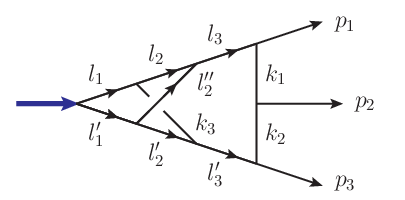
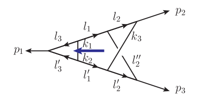
First we consider the topology shown in Figure 2 from the two-loop $\operatorname{tr}(\phi^{2})$ form factor. This topology has a reflection symmetry

\mathbf{s}_{1}:\quad\{p_{1}\leftrightarrow p_{3},\ \ k_{1}\leftrightarrow k_{2},\ \ l_{2}^{\prime\prime}\leftrightarrow k_{3},\ \ l_{m}\leftrightarrow l_{m}^{\prime}\textrm{~for~}m=1,2,3\}\,.

(12)

From (11), the diagrammatic symmetry requires

\displaystyle C_{a}{\cal F}^{(0)}(p_{1},p_{2},p_{3})

\displaystyle N_{a}(l_{1},l_{2},l_{3},p_{1},p_{2},p_{3})=\mathbf{s}_{1}\big[C_{a}\,{\cal F}^{(0)}(p_{1},p_{2},p_{3})\,N_{a}(l_{1},l_{2},l_{3},p_{1},p_{2},p_{3})\big]\,.

(13)

The symmetry action of $\mathbf{s}_{1}$ on color factors is

	$\displaystyle C_{a}$	$\displaystyle=\delta^{l_{1}l_{1}^{\prime}}\tilde{f}^{l_{1}l_{2}k_{3}}\tilde{f}^{l_{1}^{\prime}l_{2}^{\prime}l_{2}^{\prime\prime}}\tilde{f}^{l_{2}l_{3}l_{2}^{\prime\prime}}\tilde{f}^{l_{2}^{\prime}l_{3}^{\prime}k_{3}}\tilde{f}^{l_{3}a_{1}k_{1}}\tilde{f}^{l_{3}^{\prime}a_{3}k_{2}}\tilde{f}^{k_{1}a_{2}k_{2}}\,,$		(14)
	$\displaystyle\Rightarrow\quad\mathbf{s}_{1}\left[C_{a}\right]$	$\displaystyle=\delta^{l_{1}^{\prime}l_{1}}\tilde{f}^{l_{1}^{\prime}l_{2}^{\prime}l_{2}^{\prime\prime}}\tilde{f}^{l_{1}l_{2}k_{3}}\tilde{f}^{l_{2}^{\prime}l_{3}^{\prime}k_{3}}\tilde{f}^{l_{2}l_{3}l_{2}^{\prime\prime}}\tilde{f}^{l_{3}^{\prime}a_{3}k_{2}}\tilde{f}^{l_{3}a_{1}k_{1}}\tilde{f}^{k_{2}a_{2}k_{1}}=-C_{a}\,,$		(14)

where the last identity comes from the fact the only difference between $\mathbf{s}_{1}\left[C_{a}\right]$ and $C_{a}$ is the ordering of indicies in the last $\tilde{f}$ . For the kinematics numerators, one has

		$\displaystyle\mathbf{s}_{1}\big[{\cal F}^{(0)}(p_{1},p_{2},p_{3})\big]={\cal F}^{(0)}(p_{3},p_{2},p_{1})=-{\cal F}^{(0)}(p_{1},p_{2},p_{3})\,,$		(15)
		$\displaystyle\mathbf{s}_{1}\left[N_{a}(l_{1},l_{2},l_{3},p_{1},p_{2},p_{3})\right]=N_{a}(l_{1}^{\prime},l_{2}^{\prime},l_{3}^{\prime},p_{3},p_{2},p_{1})\,.$		(16)

As a result, we get the constraint on $N_{a}$ as

N_{a}(l_{1},l_{2},l_{3},p_{1},p_{2},p_{3})=N_{a}(l_{1}^{\prime},l_{2}^{\prime},l_{3}^{\prime},p_{3},p_{2},p_{1}).

(17)

In this example, it is actually not necessary to write down the lengthy product of $\tilde{f}$ as in (14), and one can directly consider the simpler form of color factor with all internal indices contracted, expressed as³³ 3 For simplicity, we use $\tilde{f}^{a_{1}a_{2}a_{3}}$ as a short notation for $\tilde{f}^{a_{1}a_{2}a_{3}}$

C_{a}=-N_{c}^{2}\tilde{f}^{a_{1}a_{2}a_{3}},\quad\quad\mathbf{s}_{1}\left[C_{a}\right]=-N_{c}^{2}\tilde{f}^{a_{3}a_{2}a_{1}}=-C_{a}\,.

(18)

Practically, such an analysis as (18) is easier because the (simplified) color factor $C$ equals to $P\left(N_{c}\right)\tilde{f}^{a_{1}a_{2}a_{3}}$ ( $P(N_{c})$ is a polynomial of $N_{c}$ ) and the combination $\tilde{f}^{a_{1}a_{2}a_{3}}\mathcal{F}^{(0)}(p_{1},p_{2},p_{3})$ is always invariant under any symmetry operation. As a result, $N_{a}=\mathbf{s}\left[N_{a}\right]$ for any $\mathbf{s}$ , bypassing detailed analyses on $C$ and $\mathcal{F}^{(0)}$ .

However, there are exceptional situations if $P\left(N_{c}\right)=0$ , such as the topology shown in Figure 2. Consider the graph symmetry of this topology:

\mathbf{s}_{2}:\quad\{l_{2}\leftrightarrow l_{2}^{\prime\prime},\ \ k_{3}\leftrightarrow l_{2}^{\prime},\ \ p_{2}\leftrightarrow p_{3}\}\,.

(19)

Since $C_{b}=0$ , both $\mathbf{s}_{2}\big[C_{b}]=\pm C_{b}$ are mathematically allowed, and an analysis as (18) is no longer possible. One can consider the trivalent form of the color factor, after following a similar path from (13) to (17),one gets

\displaystyle\mathbf{s_{2}}\left[C_{b}\right]=\mathbf{s_{2}}\big[\tilde{f}^{l_{3}^{\prime}a_{1}l_{3}}\delta^{k_{1}k_{2}}\tilde{f}^{l_{3}l_{1}k_{1}}\tilde{f}^{l_{3}^{\prime}l_{1}^{\prime}k_{2}}\tilde{f}^{l_{1}l_{2}l_{2}^{\prime\prime}}\tilde{f}^{l_{1}^{\prime}l_{2}^{\prime}k_{3}}\tilde{f}^{l_{2}a_{2}k_{3}}\tilde{f}^{l_{2}^{\prime}a_{3}l_{2}^{\prime\prime}}\big]=C_{b}\,.

(20)

Since $\mathbf{s}_{2}\big[{\cal F}^{(0)}(p_{1},p_{2},p_{3})\big]=-{\cal F}^{(0)}(p_{1},p_{2},p_{3})$ , we obtain

N_{b}(l_{1},l_{2},l_{3},p_{1},p_{2},p_{3})=-N_{b}(l_{1},l_{2}^{\prime\prime},l_{3},p_{1},p_{3},p_{2})\,.

(21)

One should be particularly careful about the minus sign on the RHS.

As a comparison, Figure 2 has another symmetry $\mathbf{s}_{3}$ :

\mathbf{s}_{3}:\qquad\{p_{2}\leftrightarrow p_{3},\,k_{1}\leftrightarrow k_{2},\,l_{2}^{\prime\prime}\leftrightarrow k_{3},\,l_{m}\leftrightarrow l_{m}^{\prime}\textrm{~for~}m=1,2,3\}\,.

(22)

In this case, one has

\displaystyle\mathbf{s_{3}}\left[C_{b}\right]

\displaystyle=\mathbf{s}_{3}\big[\tilde{f}^{l_{3}^{\prime}a_{1}l_{3}}\delta^{k_{1}k_{2}}\tilde{f}^{l_{3}l_{1}k_{1}}\tilde{f}^{l_{3}^{\prime}l_{1}^{\prime}k_{2}}\tilde{f}^{l_{1}l_{2}l_{2}^{\prime\prime}}\tilde{f}^{l_{1}^{\prime}l_{2}^{\prime}k_{3}}\tilde{f}^{l_{2}a_{2}k_{3}}\tilde{f}^{l_{2}^{\prime}a_{3}l_{2}^{\prime\prime}}\big]=-C_{b}\,,

(23)

and thus

N_{b}(l_{1},l_{2},l_{3},p_{1},p_{2},p_{3})=N_{b}(l_{1}^{\prime},l_{2}^{\prime},l_{3}^{\prime},p_{1},p_{3},p_{2})\,.

(24)

Note that there is no minus sign, different from (21), which indicates that for those topologies with zero color factors, one should be cautious about the symmetry conditions.

As we will see in the construction in Section 3, the application of these symmetry constraints can usually fix a large number of parameters in the numerator ansatz.

2.3 Full-color unitarity-cut constraints

To fix the remaining parameters and to ensure that the ansatz provides a physical integrand, we apply generalized unitarity cuts Bern:1994zx; Bern:1994cg; Britto:2004nc. The idea of the generalized unitarity method is that when performing unitarity cuts, i.e. setting certain internal lines to be on-shell

\frac{i}{l^{2}}\stackrel{{\scriptstyle\text{ cut }}}{{\longrightarrow}}2\pi\delta_{+}\left(l^{2}\right)\,,

(25)

the loop amplitude or form factor will be factorized as products of simpler on-shell building blocks, such as tree-level amplitudes and form factors. If a integrand is consistent with a spanning set of cuts (thus all possible cuts), the integrand is then guaranteed to be the correct physical result.

Below we first explain how we perform the full-color cuts by the color decomposition of the cut integrands. Then we discuss the general color-stripped cuts such as the simplest maximal cuts as well as the most complicated quadruple cuts at three loops.

1) The color decomposition of cut integrand

When performing a full-color cut, the integrand under the cut should reproduce the product of color-dressed blocks as

\sum_{\sigma}\sum_{\Gamma_{i}}\int\prod_{j=1}^{\ell}\frac{\mathrm{d}^{D}l_{j}}{(2\pi i)^{D}}\frac{1}{S_{i}}\sigma\cdot\frac{C_{i}{\cal F}_{\mathcal{O},n}^{(0)}N_{i}}{\prod_{\alpha_{i}}P^{2}_{\alpha_{i}}}\bigg|_{\{l_{\rm c}^{2}\shortrightarrow 0\}}=\int\mathrm{dPS}_{\{l_{\rm c}\}}\int\mathrm{d}\eta_{\{l_{\rm c}\}}\textbf{{F}}^{(0)}\prod_{I}\textbf{{A}}^{(0)}_{I}\,,

(26)

where $\{l_{c}\}$ is the list of internal cut lines, $\mathrm{dPS}$ represents the phase space measure, and the Grassman integration over $\mathrm{d}\eta$ serves to sum over internal states.

In practice, it is convenient to perform color decomposition for (26), such that only color-ordered tree amplitudes or form factors are needed as blocks. To illustrate this, we consider a double cut in the $s_{12}$ channel for full-color form factor $\textbf{{F}}^{(1)}_{\operatorname{tr}(\phi^{2}),3}$ , as shown in Figure 3(a).

We first consider the tree product on the RHS of (26), which can be explicitly given as

\text{Full-color cut}:\ \int\prod_{i=1}^{2}\mathrm{d}^{4}\eta_{l_{i}}\textbf{{F}}^{(0),\mathrm{MHV}}_{\operatorname{tr}(\phi^{2}),3}(-l_{1},-l_{2},p_{3})\textbf{{A}}^{(0),\mathrm{MHV}}_{4}(l_{1},l_{2},p_{1},p_{2})\,,

(27)

where we omit the phase space measure for simplicity. The tree blocks take the standard single-trace color-decomposition form Mangano:1990by:

	$\displaystyle\textbf{{F}}_{\operatorname{tr}(\phi^{2}),3}^{(0)}(-l_{1},-l_{2},p_{3})$	$\displaystyle=\sum_{\sigma_{1}\in S_{3}/\mathbb{Z}_{3}}\operatorname{tr}(\sigma_{1}(a_{l_{1}}a_{l_{2}}a_{3}))\mathcal{F}^{(0)}_{\operatorname{tr}(\phi^{2}),3}(\sigma_{1}\{-l_{1},-l_{2},p_{3}\})\,,$		(28)
	$\displaystyle\textbf{{A}}_{4}^{(0)}(l_{2},l_{1},p_{1},p_{2})$	$\displaystyle=\sum_{\sigma_{2}\in S_{4}/\mathbb{Z}_{4}}\operatorname{tr}(\sigma_{2}(a_{l_{2}}a_{l_{1}}a_{1}a_{2}))\mathcal{A}^{(0)}_{4}(\sigma_{2}\{l_{2},l_{1},p_{1},p_{2}\})\,,$		(29)

where we use the short notation $\operatorname{tr}(abc)$ for $\operatorname{tr}(T^{a}T^{b}T^{c})$ . As a result, the product in (27) can also be decomposed according to trace-color factor as

\text{Full-color Cut}:\ \sum_{\sigma_{1}\times\sigma_{2}}\operatorname{tr}(\sigma_{1}(a_{l_{1}}a_{l_{2}}a_{3}))\operatorname{tr}(\sigma_{2}(a_{l_{2}}a_{l_{1}}a_{1}a_{2}))\mathcal{K}(\sigma_{1},\sigma_{2})\,,

(30)

with $\mathcal{K}$ representing the product of color-stripped building blocks:

\mathcal{K}(\sigma_{1},\sigma_{2})=\int\prod_{i=1}^{2}\mathrm{d}^{4}\eta_{l_{i}}\mathcal{F}^{(0)}_{\operatorname{tr}(\phi^{2}),3}(\sigma_{1}\{-l_{1},-l_{2},p_{3}\})\mathcal{A}^{(0)}_{4}(\sigma_{2}\{l_{2},l_{1},p_{1},p_{2}\})\,.

Figure 3(b) and 3(c) show two configurations of such color-stripped cuts, corresponding to color factors $\operatorname{tr}(a_{l_{1}}a_{l_{2}}a_{3})\operatorname{tr}(a_{l_{2}}a_{l_{1}}a_{1}a_{2})$ and $\operatorname{tr}(a_{l_{1}}a_{l_{2}}a_{3})\operatorname{tr}(a_{l_{2}}a_{2}a_{l_{1}}a_{1})$ , respectively.

Next we can consider the LHS of (26) given by the ansatz. Similarly, the color factor $C_{i}$ in the ansatz can also be expanded in terms of the same trace color factors $\operatorname{tr}(\sigma_{1})\operatorname{tr}(\sigma_{2})$ as mentioned above. Concretely, there are three trivalent graphs contributing in this cut example, as shown in Figure 4. The color factors of the three trivalent graphs can be naturally factorized under the cuts as the product of color factors of sub-tree graphs as

	$\displaystyle C^{\rm(a)}=C^{\rm(a)}_{\textbf{{F}}_{3}}C^{\rm(a)}_{\textbf{{A}}_{4}}=(\tilde{f}^{a_{3}k_{2}l_{2}}\delta^{k_{2}l_{1}})(\tilde{f}^{l_{1}a_{1}k_{1}}\tilde{f}^{k_{1}a_{2}l_{2}})\,,$		(31)
	$\displaystyle C^{\rm(b)}=C^{\rm(b)}_{\textbf{{F}}_{3}}C^{\rm(b)}_{\textbf{{A}}_{4}}=(\tilde{f}^{a_{3}k_{2}l_{2}}\delta^{k_{2}l_{1}})(\tilde{f}^{l_{1}a_{2}k_{1}}\tilde{f}^{k_{1}a_{1}l_{2}})\,,$
	$\displaystyle C^{\rm(c)}=C^{\rm(c)}_{\textbf{{F}}_{3}}C^{\rm(c)}_{\textbf{{A}}_{4}}=(\tilde{f}^{a_{3}k_{2}l_{2}}\delta^{k_{2}l_{1}})(\tilde{f}^{a_{2}a_{1}k_{1}}\tilde{f}^{k_{1}l_{2}l_{1}})\,.$

For the color factors of trivalent sub-tree graphs, such as $C^{\rm(a)}_{\textbf{{F}}_{3}}$ and $C^{\rm(a)}_{\textbf{{A}}_{4}}$ , one can also extract proper trace color components. For example, to reproduce the contribution to the product of trace color factors $\mathcal{T}_{*}=\operatorname{tr}(a_{l_{1}}a_{l_{2}}a_{p_{3}})\operatorname{tr}(a_{l_{2}}a_{l_{1}}a_{p_{1}}a_{p_{2}})$ as for Figure 3(b), we have

		$\displaystyle C^{\rm(a)}_{\textbf{{F}}_{3}}\rightarrow(+1)\operatorname{tr}(a_{l_{1}}a_{l_{2}}a_{3}),\qquad C^{\rm(a)}_{\textbf{{A}}_{4}}\rightarrow(+1)\operatorname{tr}(a_{l_{2}}a_{l_{1}}a_{1}a_{2})\,,$		(32)
		$\displaystyle C^{\rm(b)}_{\textbf{{F}}_{3}}\rightarrow(+1)\operatorname{tr}(a_{l_{1}}a_{l_{2}}a_{3}),\qquad C^{\rm(b)}_{\textbf{{A}}_{4}}\rightarrow(0)\operatorname{tr}(a_{l_{2}}a_{l_{1}}a_{1}a_{2})\,,$
		$\displaystyle C^{\rm(c)}_{\textbf{{F}}_{3}}\rightarrow(+1)\operatorname{tr}(a_{l_{1}}a_{l_{2}}a_{3}),\qquad C^{\rm(c)}_{\textbf{{A}}_{4}}\rightarrow(-1)\operatorname{tr}(a_{l_{2}}a_{l_{1}}a_{1}a_{2})\,.$

From (32), one can get:

\{C^{\rm(a)},C^{\rm(b)},C^{\rm(c)}\}\big|_{\mathcal{T}_{*}}=\{1,0,-1\}\,.

(33)

With the above decompositions, we obtain a color-stripped version of (26) by selecting certain color orderings. For example, for Figure 3(b), selecting the component associated to color factor $\mathcal{T}_{*}$ , one has the color-stripped unitarity relation:

	$\displaystyle{\cal F}_{\operatorname{tr}(\phi^{2}),3}^{(0)}$	$\displaystyle\Bigl(\hskip-5.69046pt\begin{tabular}[]{c}{\includegraphics[width]{figure/oneloopdiagramIn1.eps}}\end{tabular}\hskip-11.38092pt\times(+1)N^{\rm(a)}+\hskip-5.69046pt\begin{tabular}[]{c}{\includegraphics[width]{figure/oneloopdiagramIn3.eps}}\end{tabular}\hskip-11.38092pt\times(-1)N^{\rm(c)}\Bigr)$
		$\displaystyle=\int\prod_{i=1}^{2}\mathrm{d}^{4}\eta_{l_{i}}\mathcal{F}^{(0)}_{\operatorname{tr}(\phi^{2}),3}(-l_{1},-l_{2},p_{3})\mathcal{A}^{(0)}_{4}(l_{2},l_{1},p_{1},p_{2})\,,$		(36)

where the signs in front of $N^{\rm(a)}$ and $N^{\rm(c)}$ are given by (33). The same consideration can be easily applied to other orderings, including the non-planar cut in Figure 3(c). The generalization to generic high-loop cases is also straightforward.

2) Maximal cuts

A special class of cuts is the maximal cuts where all possible propagators are put on-shell Britto:2004nc; Bern:2007ct. In this case, only one topology contributes to the cut and one has

{\cal F}_{\mathcal{O},n}^{(0)}\,N_{i}\Big|_{P^{2}_{\alpha_{i}}\shortrightarrow 0}=\int\left(\mathrm{d}\eta_{\{l_{\rm c}\}}\right)^{4}\mathcal{F}^{(0)}_{{\cal O},{\rm min}}\prod_{\rm I}\mathcal{A}^{(0)}_{3,\mathrm{I}}\,,

(37)

where $\mathcal{F}^{(0)}_{{\cal O},{\rm min}}$ is the minimal form factor and $\mathcal{A}_{3}^{(0)}$ are three-point amplitudes. Sometimes it is possible to apply the maximal-cut without actually calculating the product of three-point tree amplitudes. In such cases, one can apply the rung-rule Bern:1998ug to guess the numerators and compare them with the ansatz under maximal cuts.

Maximal cuts can be regarded as a property of each individual diagram, similar to the graph symmetry constraint in Section 2.2. In practice, it is often used before applying more complicated cuts.

3) General non-maximal cuts

A complete set of unitarity condition involves more general unitarity cuts, in which less propagators are put on-shell such as examples given in Figure 5. For the three-loop form factors, the most complicated cuts are the quadruple cuts, where only four propagators are cut and the full integrand factorizes as the product of two tree blocks. Two such cuts are shown in Figure 5(c) and 5(d). Non-trivial tree building blocks are involved in such cases, for example, the tree product for the case of Figure 5(d) can be given as

$\displaystyle\int\prod_{i=1}^{4}\left(d\eta_{l_{i}}\right)^{4}\Big[$	$\displaystyle\mathcal{F}_{\mathcal{O},5}^{(0),\mathrm{MHV}}\left(p_{1},-l_{1},-l_{2},-l_{3},-l_{4}\right)\mathcal{A}_{6}^{(0),\mathrm{NNMHV}}\left(p_{2},l_{1},l_{4},p_{3},l_{3},l_{2}\right)$	(38)
$\displaystyle+$	$\displaystyle\mathcal{F}_{\mathcal{O},5}^{(0),\mathrm{NMHV}}\left(p_{1},-l_{1},-l_{2},-l_{3},-l_{4}\right)\mathcal{A}_{6}^{(0),\mathrm{NMHV}}\left(p_{2},l_{1},l_{4},p_{3},l_{3},l_{2}\right)$
$\displaystyle+$	$\displaystyle\mathcal{F}_{\mathcal{O},5}^{(0),\mathrm{NNMHV}}\left(p_{1},-l_{1},-l_{2},-l_{3},-l_{4}\right)\mathcal{A}_{6}^{(0),\mathrm{MHV}}\left(p_{2},l_{1},l_{4},p_{3},l_{3},l_{2}\right)\Big]\,.$

The MHV tree-level amplitudes are standard Parke-Taylor form Parke:1986gb, and MHV form factors of $\mathcal{O}=\operatorname{tr}(\phi^{L})$ take simple Parke-Taylor-like form (see e.g. Yang:2019vag). As for the N^kMHV amplitudes and form factors, they can be computed via BCFW on-shell recursion Britto:2005fq or CSW vertex expansion Cachazo:2004kj methods.

The tree products can be compared with the cut of CK-dual ansatz, similar to (36). For three-loop cases, the ansatz cut-diagrams have typically a total number of order $\sim O(100)$ . Thus the quadruple cuts provide very non-trivial constraints on the results as well as the most stringent checks.

4) On $D$ -dimensional cuts

Since we use dimensional regularization and the loop momenta are $D$ -dimensional, one should in principle apply unitarity cuts in $D$ dimensions. In this respect, we have checked our results by applying $D$ -dimensional cuts that contain four-point sub-amplitudes, following the strategy in Bern:2010tq. Although it would be interesting to consider further for a complete set of $D$ -dimensional cuts, we would like to make the following two remarks that strongly support the completeness of our results:

•

First, the dual Jacobi relations that relate numerators of different diagrams are expected to hold in any dimension, and the ansatz of the numerators are given in terms of Lorentz products (not spinor products) which are in a form valid in general dimensions.
•

Second, we have evaluated the full-color form factors numerically, as will be discussed later in Section 5. Our results give consistent full-color IR divergences as well as the planar finite remainder function from a bootstrap computation Dixon:2020bbt. A possibly missing $D$ -dimensional contribution (such as $\mu^{2}$ -term integral) would easily modify (the divergent or finite part of) the results and thus would lead to inconsistency.

3 Constructing three-loop form factor integrands

In this section, we apply the strategy described in the previous section to construct the full-color integrands of three-loop three-point form factors:

\mathcal{F}_{\mathcal{O}}(1,2,3;q)=\int d^{D}xe^{-iq\cdot x}\langle\Phi_{1}(p_{1})\Phi_{2}(p_{2})\Phi_{3}(p_{3})|\mathcal{O}(x)|0\rangle\,,

(39)

where $p_{i}^{2}=0,i=1,2,3,$ and $q^{2}=(p_{1}+p_{2}+p_{3})^{2}\neq 0$ . We consider two types of operators: one is $\operatorname{tr}(\phi^{2})$ which is also a component of the stress-tensor supermultiplet, and the other is the length-three half-BPS operator ${\rm tr}(\phi^{3})$ .

3.1 Warm-up: Two-loop three-point form factor of $\operatorname{tr}(\phi^{2})$

As a warm-up example, let us briefly revisit the simpler case—the two-loop three-point form factor of the stress-tensor supermultiplet Boels:2012ew. Here we will obtain a more general CK-dual solution that contains four free parameters.

Constructing ansatz

(1)

Trivalent topologies

Following the criteria of selecting trivalent topology in Section 2.1, one finds that there are six contributed topologies, given by (1)–(6) in Figure 6.

Figure 6: Trivalent topologies for the two-loop form factor of 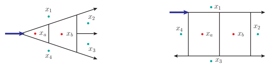$\operatorname{tr}(\phi^{2})$ .

Figure 7: Master graphs for two-loop $\operatorname{tr}(\phi^{2})$ form factor.

(2)

Jacobi relations and master numerators

By generating the dual Jacobi relations, one can find it is possible to choose two planar topologies as master topologies, as shown in Figure 7.⁴⁴ 4 Note that in this case it is also possible to choose one non-planar graph, that is Figure 6(5), as the single master topology. Other numerators can be determined from master numerators $N_{1}$ and $N_{4}$ by the following dual Jacobi relations:

		$\displaystyle N_{2}(p_{1},p_{2},p_{3})=N_{1}(p_{2},p_{3},p_{1})+N_{1}(p_{3},p_{2},p_{1})\,,$
		$\displaystyle N_{5}(p_{1},p_{2},p_{3},\ell)=N_{1}(p_{1},p_{2},p_{3})-N_{4}(p_{1},p_{2},p_{3},\ell)\,,$
		$\displaystyle N_{3}(p_{1},p_{2},p_{3})=N_{2}(p_{1},p_{2},p_{3})\,,\qquad N_{6}(p_{1},p_{2},p_{3},\ell)=N_{4}(p_{1},p_{2},p_{3},\ell)\,.$		(40)

(3)

Master numerators and the Ansatz

Taking advantage of the planarity of master graphs, we apply zone variables to parametrize the momenta, which are defined explicitly in Figure 7. The master numerators are polynomials of zone variables with degree three. Moreover, as described in Section 2.1, the good UV property of ${\cal N}=4$ SYM provides strong power-counting constraints on the loop momenta dependence in master numerators: for $N_{1}$ of the first master in Figure 7, $x_{b}$ can appear at most once in Lorentz products, so $(x_{ib}^{2})^{1}$ , with $i=1,2,3,4$ , is allowed, and any term containing $x_{a}$ is forbidden; while for the other master numerator $N_{4}$ , $x_{a}$ can appear at most once. With these conditions, we obtain an ansatz for two master numerators with 68 parameters in total.

Solving ansatz

Next, to solve the ansatz, we impose various conditions as follows.

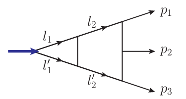
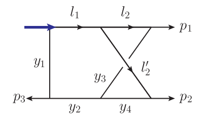
(1)

First we apply symmetry constraints on all topologies. As mentioned in Section 2.2, if the color factor is non-zero, it is straightforward to write down conditions from diagrammatic symmetries for three-point form factors; otherwise, a more detailed analysis is required.

Specifically, color factors of (1)–(5) in Figure 6 are not zero, whereas the color factor of Figure 6(6) is zero, and below we choose (1) and (6) as examples. For Figure 6(1), one has a symmetry $\mathbf{s}_{1}:\{p_{1}\leftrightarrow p_{3},l_{1,2}\leftrightarrow l_{1,2}^{\prime}\}$ . Such a symmetry leads to

C_{1}\mathcal{F}^{(0)}N_{1}(l_{1},l_{2},p_{1},p_{2},p_{3})=\mathbf{s}_{1}\big[C_{1}\mathcal{F}^{(0)}N_{1}(l_{1},l_{2},p_{1},p_{2},p_{3})\big]\,.

(41)

Here we have

		$\displaystyle\mathbf{s}_{1}\big[C_{1}]=\mathbf{s}_{1}[2N_{c}^{2}\tilde{f}^{a_{1}a_{2}a_{3}}]=2N_{c}^{2}\tilde{f}^{a_{3}a_{2}a_{1}}=-C_{1};$		(42)
		$\displaystyle\mathbf{s}_{1}[\mathcal{F}^{(0)}(p_{1},p_{2},p_{3})]=\mathcal{F}^{(0)}(p_{3},p_{2},p_{1})=-\mathcal{F}^{(0)}(p_{1},p_{2},p_{3})\,,$		(42)

resulting in

N_{1}(l_{1},l_{2},p_{1},p_{2},p_{3})=N_{1}(l_{1}^{\prime},l_{2}^{\prime},p_{3},p_{2},p_{1})\,.

(43)

For Figure 6(6), since its color factor is zero, it is necessary to consider the full trivalent product form. Consider the symmetry $\mathbf{s}_{2}:\{p_{1}\leftrightarrow p_{2},l_{2}\leftrightarrow l_{2}^{\prime},y_{3}\leftrightarrow y_{4}\}$ , one gets

\displaystyle\mathbf{s}_{2}\left[C_{6}\right]

\displaystyle=\mathbf{s}_{2}\left[\delta^{l_{1}k_{1}}\tilde{f}^{k_{1}k_{2}a_{3}}\tilde{f}^{l_{1}l_{2}l_{2}^{\prime}}\tilde{f}^{k_{2}k_{3}k_{4}}\tilde{f}^{l_{2}a_{1}k_{3}}\tilde{f}^{l_{2}^{\prime}a_{2}k_{4}}\right]=C_{6}\,,

(44)

so that

N_{6}(l_{1},l_{2},p_{1},p_{2},p_{3})=-N_{6}(l_{1},l_{2}^{\prime},p_{2},p_{1},p_{3})\,.

(45)

After considering all symmetries, 68 free parameters are reduced to only 16.

(2)

Next we apply generalized unitarity cuts, where two most constraining planar cuts are shown in Figure 9(a)–9(b). The expressions of tree products are

	$\displaystyle\hskip-2.5pt\text{Cut-(a)}:\ \int\prod_{i=1}^{3}\left(d\eta_{l_{i}}\right)^{4}\Big[$	$\displaystyle\mathcal{F}_{\operatorname{tr}(\phi^{2}),3}^{(0),\mathrm{MHV}}\left(-l_{1},-l_{2},-l_{3}\right)\mathcal{A}_{6}^{(0),\mathrm{NMHV}}\left(p_{1},p_{2},p_{3},l_{3},l_{2},l_{1}\right)$		(46)
	$\displaystyle+$	$\displaystyle\mathcal{F}_{\operatorname{tr}(\phi^{2}),3}^{(0),\mathrm{NMHV}}\left(-l_{1},-l_{2},-l_{3}\right)\mathcal{A}_{6}^{(0),\mathrm{MHV}}\left(p_{1},p_{2},p_{3},l_{3},l_{2},l_{1}\right)\Big]\,,$		(46)

	$\displaystyle\hskip-2.5pt\text{Cut-(b)}:\ \int\prod_{i=1}^{3}\left(d\eta_{l_{i}}\right)^{4}\Big[$	$\displaystyle\mathcal{F}_{\operatorname{tr}(\phi^{2}),4}^{(0),\mathrm{MHV}}\left(p_{1},-l_{1},-l_{2},-l_{3}\right)\mathcal{A}_{5}^{(0),\mathrm{NMHV}}\left(p_{2},p_{3},l_{3},l_{2},l_{1}\right)$		(47)
	$\displaystyle+$	$\displaystyle\mathcal{F}_{\operatorname{tr}(\phi^{2}),4}^{(0),\mathrm{NMHV}}\left(p_{1},-l_{1},-l_{2},-l_{3}\right)\mathcal{A}_{5}^{(0),\mathrm{MHV}}\left(p_{2},p_{3},l_{3},l_{2},l_{1}\right)\Big]\,.$		(47)

These two cuts can fix 12 parameters among the 16 parameters.

(3)

Finally, one can check the integrand solution with four free parameters satisfies all other cuts and all the dual Jacobi relations. Hence, this four-parameter solution is the final solution that manifests CK-dual structure and is consistent with all unitarity conditions.

The master-numerator solution with four parameters takes the following form:

$\displaystyle N_{1}=$	$\displaystyle x_{14}^{2}x_{13}^{2}x_{23}^{2}/2$	(48)
	$\displaystyle-c_{1}\bigl(S_{\rm p,3}\big(x_{b3}^{2}-x_{b4}^{2}\big)+S_{\rm p,2}\big(x_{b2}^{2}-x_{b3}^{2}\big)+S_{\rm p,1}(x_{b1}^{2}-x_{b2}^{2}\big)\bigr)$
	$\displaystyle-c_{2}\bigl(S_{\rm s,3}\big(x_{b3}^{2}-x_{b4}^{2}\big)+S_{\rm s,2}\big(x_{b2}^{2}-x_{b3}^{2}\big)+S_{\rm s,1}(x_{b1}^{2}-x_{b2}^{2}\big)\bigr)$
$\displaystyle N_{4}=$	$\displaystyle x_{13}^{2}(x_{13}^{2}x_{24}^{2}+(x_{13}^{2}-x_{14}^{2})(x_{1a}^{2}-x_{2a}^{2})+x_{24}^{2}(x_{1a}^{2}-x_{3a}^{2}))/2$
	$\displaystyle+c_{1}S_{\rm p,3}\bigl(x_{a3}^{2}-x_{a4}^{2}\bigr)+c_{2}S_{\rm s,3}\bigl(x_{a3}^{2}-x_{a4}^{2}\bigr)$
	$\displaystyle+c_{3}S_{\rm p,3}\bigl(x_{a4}^{2}-x_{a1}^{2}\bigr)+c_{4}S_{\rm s,3}\bigl(x_{a4}^{2}-x_{a1}^{2}\bigr)$

where $c_{1,2,3,4}$ denote the four parameters and $S_{\mathrm{p},i}$ , $S_{\mathrm{s},i}$ are simple functions of Mandelstam variables $s_{ij}$ , for example $S_{\rm p,3}=s_{12}(s_{23}-s_{13})$ . See more details in Appendix A.

We mention that our result reproduces the result in Boels:2012ew when setting $c_{1,2,3,4}=0$ . Of course, there is no physical requirement that forces $c_{i}$ to be 0. We will show in Section 3.4 that these parameters come from a special deformation of the integrand and they cancel at the integrand level.

Final solution

The final two-loop full-color integrand reads

{\cal F}_{{\rm tr}(\phi^{2}),3}^{(2)}={\cal F}_{{\rm tr}(\phi^{2}),3}^{(0)}\sum_{\sigma_{e}}{\text{sgn}(\sigma_{e})}\sum_{i=1}^{6}\int\prod_{j=1}^{3}d^{D}\ell_{j}{1\over S_{i}}\,\sigma_{e}\cdot{C_{i}\,N_{i}\over\prod_{\alpha_{i}}P^{2}_{\alpha_{i}}}\,,

(49)

where the various factors are given in Appendix A. The permutation operator $\sigma_{e}\in S_{3}$ acts on the three external momenta and color indices in $N_{i},P^{2}_{\alpha_{i}}$ and $C_{i}$ . Notice that the tree-level form factor is factorized out and not permuted by $\sigma_{e}$ , which is different from (8); this requires a compensation which is responsible for the extra $\text{sgn}(\sigma_{e})$ factor. The $\text{sgn}(\sigma_{e})$ is +1/-1 for even/odd permutation $\sigma_{e}$ respectively, rising from the fact that the tree-level form factor gives a $\text{sgn}(\sigma_{e})$ when permuting external lines. .

Finally, we comment that as we will see in the three-loop cases, the existence of free parameters in final CK-dual solutions appears to be a more general feature.

3.2 Three-loop three-point form factor of $\operatorname{tr}(\phi^{2})$

In this subsection, we construct the full-color three-loop integrand for the three-point form factor of the stress-tensor supermultiplet.

CK-dual ansatz

(1)

Trivalent topologies The first step is to construct three-loop trivalent topologies. Using the same selection rule mentioned in Section 2.1, we find that there are in total 29 topologies, which are listed in Figure 10.
(2)

Jacobi relations and master numerators

We assume the form factor can be expressed in the form of (8), where the numerators $N_{i},i=1,...,29,$ satisfy dual Jacobi relations. By inspecting the dual Jacobi relations for all 29 trivalent topologies, we find that the minimal number of master graphs is two. A convenient choice is to select $N_{1},N_{2}$ (both are planar) as master numerators, and their topologies are shown in Figure 11 respectively.
(3)

Ansatz for master numerators

As for the ansatz for master numerators, similar to the two-loop case, we define zone variables as in Figure 11. The ansatz should be a degree-four polynomial of zone variables, and the power-counting constraints are as follows. For $N_{1}$ , $x_{a},x_{c}$ can appear at most once, so both $(x^{2}_{ai})^{1},(x^{2}_{ci})^{1}$ , with $i=1,2,3,4$ , and $(x^{2}_{ac})^{1}$ are allowed; any term containing $x_{b}$ or more than one $x_{a}$ or $x_{c}$ , such as $(x^{2}_{ac})^{2},(x^{2}_{a1})^{2}$ are forbidden. For $N_{2}$ , only $x_{b}$ can appear and can appear at most twice, so only $x^{2}_{bi}$ can appear, with possible power $2,1,0$ . With these requirements, the total number of parameters is 316: 201 for the first numerator and 115 for the second.

Solving ansatz

Given the integrand ansatz, we now consider diagrammatic symmetries and unitarity conditions to solve for the parameters.

(1)

We first apply the symmetries. Examples of applying symmetry conditions for three-loop topologies have been given in Section 2.2, and we skip details here. After applying symmetry conditions of all topologies, an ansatz with only 105 parameters is obtained. One can see that the symmetry conditions provide strong constraints and can substantially reduce the number of parameters.
(2)

Next we apply unitarity-cut constraints. In this case, we directly apply the most constraining cuts, i.e. the quadruple cuts discussed in Section 2.3, such as (c) and (d) in Figure 5. With these cuts, only 24 parameters remains unsolved.
(3)

Finally, one can check that the solution with 24 free parameters satisfies all the dual Jacobi relations as well as other unitarity cuts, thus the 24-parameter solution is indeed physical. It is interesting and a little surprising that the final solution still contains a quite large number of free parameters, which we will discuss more in Section 3.4.

Final solutions

The full-color integrand for $\operatorname{tr}(\phi^{2})$ form factor at three loops can be given as follows:

\textbf{{F}}_{{\rm tr}(\phi^{2}),3}^{(3)}={\cal F}_{{\rm tr}(\phi^{2}),3}^{(0)}\sum_{\sigma_{e}}{\text{sgn}(\sigma_{e})}\sum_{i=1}^{29}\int\prod_{j=1}^{3}d^{D}\ell_{j}{1\over S_{i}}\,\sigma_{e}\cdot{C_{i}\,N_{i}\over\prod_{\alpha_{i}}P^{2}_{\alpha_{i}}}\,,

(50)

where the notations have been explained in the previous two-loop case, and the explicit expressions of various factors can be found in the ancillary files in Lin:2021kht.⁵⁵ 5 In the ancillary files in Lin:2021kht, we explain how the permutation acts on the numerators. In particular, the $\sigma_{e}\in S_{3}$ acting on $N_{i}$ may give an extra sign in Lin:2021kht. Here in (50), we explicitly extract this possible sign by introducing the signature function $\text{sgn}(\sigma_{e})$ .

3.3 Three-loop three-point form factor of ${\rm tr}(\phi^{3})$

In this subsection, we construct the full-color three-loop integrand for the three-point form factor of the half-BPS operator ${\rm tr}(\phi^{3})$ . Compared with the previous construction for the form factor of $\operatorname{tr}(\phi^{2})$ , the $\operatorname{tr}(\phi^{3})$ case is simpler, partly because of the smaller number of propagators for each cubic graph.

Constructing ansatz

We now provide some details of CK-ansatz construction of the three-point form factor of $\operatorname{tr}(\phi^{3})$ .

(1)

Trivalent topologies

Also following the topology selection rule described in Section 2.1, there are 26 topologies. Twenty of them, (1)–(20) in Figure 12, the operator vertex is connected to three internal lines; they will be called range-three topologies. While in the remaining six topologies, (21)–(26) i.e. the last row in Figure 12, the operator vertex is connected to only two internal lines, and one of the external lines is decoupled in the interaction; they will be called range-two topologies.

Figure 12: Trivalent topologies for the three-loop form factor of $\operatorname{tr}(\phi^{3})$ .
(2)

Jacobi relations and master numerators

Since we generate dual Jacobi relations from propagators not directly attached to the $q^{2}$ vertex, for high-length operator (length $\geq$ 3) the Jacobi relations for diagrams with different interacting ranges are decoupled. Thus, numerators $N_{i}$ with $i=1,\ldots,20$ and $i=21,\ldots,26$ satisfy two sets of decoupled dual Jacobi relations. Accordingly, the master numerators should be selected separately.

For the range-three topologies, we choose $N_{1},N_{2},N_{3}$ as planar master numerators; while for the range-two graphs, we choose $N_{21}$ as a master. Although the choice of masters is not unique, we choose above topologies mainly because they are planar and mostly symmetric, which are nice properties in the ansatz construction.⁶⁶ 6 It is possible to choose only three masters but involving non-planar graphs, such as $N_{9},N_{11}$ and $N_{21}$ .
(3)

Ansatz for master numerators

Figure 13: Master graphs for three-loop $\operatorname{tr}(\phi^{3})$ form factor.

The master graphs and the defintion of zone variables are shown in Figure 13. The power-counting constraints of these four masters are: for $N_{1}$ , only $x^{2}_{ci}$ can appear, with possible power $2,1,0$ ; for $N_{2}$ , both $(x^{2}_{ai})^{1},(x^{2}_{ci})^{1}$ , and $(x^{2}_{ac})^{1}$ are allowed; for $N_{3}$ , both $(x^{2}_{ai})^{1},(x^{2}_{bi})^{1}$ , and $(x^{2}_{ab})^{1}$ are allowed; in the end we have only $x^{2}_{bi}$ with possible power $1,0$ . Given these power-counting constraints, we can write down an ansatz as a linear combination of monomial with undetermined coefficients. The total number of parameters to fix is 295.

Solving ansatz

(1)

In this case, we first impose conditions for each master graphs individually, including the maximal cuts and symmetry constraints.

For maximal cuts, we can use rung-rule Bern:1998ug; Bern:2010tq to determine the “irreducible” part (i.e. the maximal-cut-detectable part) of each master numerator, reading

0,\quad-x_{24}^{2}x_{a4}^{2}x_{1c}^{2},\quad-x_{2b}^{2}x_{3a}x_{14}^{2}+x_{3a}x_{1b}^{2}x_{14}^{2}+x_{4a}x_{2b}^{2}x_{14}^{2},\quad x_{2b}^{2}x_{13}\,,

(51)

and 19 parameters can be fixed after applying maximal cuts.

Furthermore, the symmetries of master topologies themselves can be considered, solving 92 more parameters and resulting in a simpler master ansatz.

(2)

Since we can derive all other numerators based on dual Jacobi relations and master numerators, we can then apply the constraints—symmetries, dual Jacobi relations and maximal cuts—on diagrams other than masters, as described in Section 2.3.

Concretely, the symmetries of graphs other than master graphs are considered and 138 more parameters are fixed. Next all the possible dual Jacobi relations are checked, and 13 more parameters are solved. Then all the remaining maximal cuts can be considered which further fix 7 parameters. The dimension of the parameter space is thus reduced to only 26.
(3)

Finally, the constraints from other unitarity cuts are considered, involving the two quadruple cuts stated in Section 2.3 and 16 parameters can be solved. With this 10-parameter integrand, we have checked a spanning set of cuts and no further parameters can be solved. Thus, we reach the final solution for master numerators.

Final solution

The full-color integrand for $\operatorname{tr}(\phi^{3})$ form factor at three loops can be given as follows:⁷⁷ 7 As a side remark, no extra signature like ${\text{sgn}(\sigma_{e})}$ appears here because tree-level form factor ${\cal F}_{{\rm tr}(\phi^{3}),3}^{(0)}=1$ is invariant under permutation.

\textbf{{F}}_{{\rm tr}(\phi^{3}),3}^{(3)}={\cal F}_{{\rm tr}(\phi^{3}),3}^{(0)}\sum_{\sigma}\sum_{i=1}^{26}\int\prod_{j=1}^{3}d^{D}\ell_{j}{1\over S_{i}}\,\sigma\cdot{C_{i}\,N_{i}\over\prod_{\alpha_{i}}P^{2}_{\alpha_{i}}}\,,

(52)

where the various factors can also be found in anciliary files in Lin:2021kht. We only need to point out that unlike the form factor of ${\rm tr}(\phi^{2})$ , here the permutation $\sigma$ has a more complicated structure. We write $\sigma=\sigma_{i}\times\sigma_{e}$ : $\sigma_{e}\in S_{3}$ acts on external color indices and momenta as before and $\sigma_{i}\in S_{3}/\mathbb{Z}_{3}$ acts on lines directly connected to the operator vertex, because there are two inequivalent ways of connecting three internal lines to a single-trace length-three operator. About this point, further examples and explanations can be found in Section 4.1.

3.4 Free parameters and generalized gauge transformations

One very interesting finding about the integrand solutions obtained in previous subsections is that they contain a large number of free parameters. In other words, the form factor integrand lies in a large solution space that manifests CK-duality. Since we have considered a spanning set of unitarity cuts, all the solutions in the solution space should be equivalent and can be deformed from one another.⁸⁸ 8 In Section 4, we will show that all free parameters indeed cancel by simplifying the integrand properly. As we will see, such CK-reserving deformations have an origin of generalized gauge transformations and reflect new features due to the operator insertion for form factors.

From traditional gauge transformation (GT) to generalized GT

It is well-known that the traditional gauge transformations (GTs) correspond to the change of external polarization vectors. For example, amplitudes and form factors should be invariant under the following transformation of gluon polarization vectors:

\varepsilon_{i}^{\mu}\rightarrow\varepsilon_{i}^{\mu}+\alpha p_{i}^{\mu}\,,

(53)

where $\alpha$ is an arbitrary function.

Consider the four-gluon tree amplitude with the numerator expressions in (2.1), one can perform the traditional GT for $\varepsilon_{1}$ , and the numerators $N_{s,t,u}$ are not invariant but shifted as:

N_{s}\rightarrow N_{s}+\alpha\delta_{s},\quad\text{ with }\delta_{s}=N_{s}\big|_{\varepsilon_{1}\shortrightarrow p_{1}}\,,

(54)

and so are $N_{t,u}$ . An explicit calculation shows that the deformations $\delta_{s,t,u}$ satisfy

\delta_{s}=-s\mathcal{V}_{234},\quad\delta_{t}=t\mathcal{V}_{234},\quad\delta_{u}=u\mathcal{V}_{234}\,,

(55)

with $\mathcal{V}_{234}=\left(\varepsilon_{2}\cdot{\bf p}_{34}\right)\mathcal{E}_{34}+\left(\varepsilon_{3}\cdot{\bf p}_{42}\right)\mathcal{E}_{42}+\left(\varepsilon_{4}\cdot{\bf p}_{23}\right)\mathcal{E}_{23}$ , following the notation in (2.1). It is easy to check that the full amplitude in (2) is invariant.

The above transformation can be taken as a special case of generalized gauge transformation (GGT) Bern:2010ue:

N_{s}\shortrightarrow N_{s}-s\Delta,\qquad N_{t}\shortrightarrow N_{t}+t\Delta,\qquad N_{u}\shortrightarrow N_{u}+u\Delta\,,

(56)

where $\Delta$ can be an arbitrary function while the four-gluon amplitude still remains unchanged. The traditional GT in (55) corresponds to the special choice $\Delta=\alpha\mathcal{V}_{234}$ , but a general $\Delta$ does not necessarily originates from shifting polarization vectors and thus can be defined in more general cases.

To be more explicit, let us consider embedding the four-point amplitudes into a general loop integrand like Figure 1. The following deformation of the corresponding loop-graph numerators leaves the loop integrand unchanged:

N_{s}\rightarrow N_{s}-l_{s}^{2}\Delta\,,\quad N_{t}\rightarrow N_{t}+l_{t}^{2}\Delta\,,\quad N_{u}\rightarrow N_{u}+l_{u}^{2}\Delta\,,

(57)

with $\Delta$ an arbitrary function, owing to the fact:⁹⁹ 9 In this subsection, we omit possible loop-integration measure for simplicity.

\frac{C_{s}\Delta_{s}}{l_{s}^{2}\prod^{\prime}_{m}D_{m}}+\frac{C_{t}\Delta_{t}}{l_{t}^{2}\prod^{\prime}_{m}D_{m}}+\frac{C_{u}\Delta_{u}}{l_{u}^{2}\prod^{\prime}_{m}D_{m}}\ \propto\ (C_{s}-C_{t}-C_{u})=0\,,

(58)

where $\Delta_{s,t,u}=l_{s,t,u}^{2}\Delta$ and $\prod^{\prime}_{a}$ denotes the product of common propagators other than $l^{2}_{s,t,u}$ . Such a deformation belongs to generalized gauge transformations at loop level.

Traditional GT for form factors and operator-induced GGT

For form factors, one can conduct a parallel analysis. The simplest tree-level example is the three-point form factor of $\operatorname{tr}(\phi^{2})$ . It is easy to write down the following Feynman diagrams

\begin{aligned} \includegraphics[height]{figure/F3tree.eps}\end{aligned}\,,

(59)

so that the full-color form factor is

\textbf{{F}}^{(0)}_{\operatorname{tr}(\phi^{2}),3}=\left(\frac{C_{s_{13}}N_{s_{13}}}{s_{13}}+\frac{C_{s_{23}}N_{s_{23}}}{s_{23}}\right)\,;\quad N_{s_{13}}=2\varepsilon_{3}\cdot p_{1},\ N_{s_{23}}=-2\varepsilon_{3}\cdot p_{2},

(60)

and $C_{s_{13}}=C_{s_{23}}=\tilde{f}^{a_{1}a_{2}a_{3}}$ . Note that the color factor associated to the $q^{2}$ vertex is a $\delta$ -function in color space. Performing a traditional GT similar to (53), one has

N_{s_{13}}\rightarrow N_{s_{13}}+\alpha s_{13},\quad N_{s_{23}}\rightarrow N_{s_{23}}-\alpha s_{23},

(61)

which leaves the form factor invariant.

As in the amplitude case, there are also generalized versions of GTs. Let us consider the loop diagrams of form factor of $\operatorname{tr}(\phi^{2})$ operator in Figure 14. The two diagrams have same color factors $C_{\rm a}=C_{\rm b}$ since the $q^{2}$ vertex is a $\delta$ -function. One can perform a generalized GT as

N_{\rm a}\rightarrow N_{\rm a}+l_{\rm a}^{2}\Delta,\quad N_{\rm b}\rightarrow N_{\rm b}-l_{\rm b}^{2}\Delta\,,

(62)

and it is easy to check that the full-color loop integrand is not altered for arbitrary $\Delta$ :

\frac{C_{\rm a}l_{\rm a}^{2}\Delta}{l_{\rm a}^{2}\prod^{\prime}_{m}D_{m}}+\frac{C_{\rm b}l_{\rm b}^{2}\Delta}{l_{\rm b}^{2}\prod^{\prime}_{m}D_{m}}\ \propto\ (C_{\rm a}-C_{\rm b})=0\,.

(63)

We see that for form factors, due to the insertion of local operators, a new type of generalized gauge transformations appears, where the “operator-hopping transformation” illustrated by Figure 14 plays a fundamental role that is similar to the “ $s$ -, $t$ - and $u$ -transformation” in Figure 1. Since the two types of generalized gauge transformations (GGTs), (57) and (62), originate from different types of color relations, we assign different names to distinguish them:

	$\displaystyle\eqref{eq:JacobiGT}:\qquad$	$\displaystyle\textrm{\emph{Jacobi-induced} generalized gauge transformation},$
	$\displaystyle\eqref{eq:generalGT2}:\qquad$	$\displaystyle\textrm{\emph{operator-induced} generalized gauge transformation}.$

CK-preserving deformations and cancellations of free parameters

Since there are two types of GGTs for form factors, it is possible to get a large solution space, parametrized by the parameters in integrands, compared with the amplitude cases. The existence of the solution space is due to special CK-preserving deformations, which are formed based on the two types of GGTs. Below we try to understand the roles played by these GGTs in the CK-preserving deformations and the cancellations of free parameters. For simplicity, we will consider the two-loop form factor as an example and the three-loop cases follow the same discussion.

We first explain how the free parameters can be understood as GGTs. Let us consider the two-loop numerator solutions given in Appendix A and focus on the free parameter $c_{1}$ . Without loss of generality, consider the numerator $N_{4}$ with topology shown in Figure 15(a), and the part proportional to $c_{1}$ (denoted as $N_{4}|_{c_{1}}$ ) is

N_{4}\big|_{c_{1}}=c_{1}s_{12}(s_{23}-s_{13})\big((l_{a}-p_{1}-p_{2})^{2}-(l_{a}-q)^{2}\big)\,.

(64)

One can observe that in $N_{4}|_{c_{1}}$ , all terms are proportional to certain propagators. We explain now that they can be naturally generated from GGTs.

To begin with, we notice that a Jacobi-induced GGT is illustrated in Figure 15(b), and an operator-induced GGT is shown in Figure 15(c), both of which involve the diagram shown in Figure 15(a). The first Jacobi-induced GGT leads to a deformation of $N_{4}$ proportional to $D_{\alpha}=(l_{a}-p_{1}-p_{2})^{2}$ while the second operator-induced GGT gives the $D_{\beta}=(l_{a}-q)^{2}$ term. In this example, one can specifically set $\Delta=c_{1}s_{12}(s_{23}-s_{13})$ in (57) and (62), and the involved propagators are highlighted by red color in Figure 15. Thus, $N_{4}|_{c_{1}}$ in (64) can be put in a form as $(D_{\alpha}-D_{\beta})\times\Delta$ , which originates from the two types of GGTs. One can check that the similar $c_{1}$ terms appear in the numerators of other topologies in Figure 15(b)--(c) and they cancel when adding together.¹⁰¹⁰ 10 Note that the two diagrams in (c) belong to the same topology but with different external line permutations. They cancel because the factor $s_{12}(s_{23}-s_{13})$ is anti-symmetric when permuting $p_{1}$ and $p_{2}$ .

More interestingly, such a deformation also preserves the dual Jacobi relations. For example, one can inspect the $c_{1}$ -relevant part in all $N_{i}$ given explicitly in Appendix A and directly check that no dual Jacobi relations are spoiled by $c_{i}$ deformation. Here we would like to understand this point by studying the special structure of the deformations. Consider again the aforementioned $N_{4}|_{c_{1}}$ given by (64) as an example. One notes that $N_{4}|_{c_{1}}\propto(D_{\alpha}-D_{\beta})$ where both $D_{\alpha,\beta}$ are connected to the vertex associated to the massless $p_{3}$ leg. The similar structure also exists for all other $N_{i}$ in Appendix A: focusing for instance on the $c_{1}$ deformation and the $s_{12}(s_{23}-s_{13})\equiv S_{\rm p,3}$ terms in other numerators, one always finds the structure of $(P^{2}-(P-p_{3})^{2})$ where $P^{2}$ and $(P-p_{3})^{2}$ are two propagators connected to the $p_{3}$ leg.

This structure is important for preserving dual Jacobi relations. Consider the dual Jacobi relation related to Figure 15(b), and extract the $s$ -, $t$ - and $u$ -channel sub-diagrams as

\begin{aligned} \includegraphics[width]{figure/A4treehighlighted.eps}\end{aligned}\,.

Summing up the $c_{1}$ -related deformation in the dual Jacobi relation, one finds

\left(N_{s}-N_{t}-N_{u}\right)\big|_{c_{1}}\ \propto\ \left(D_{1,s}-D_{2,s}\right)-\left(D_{1,t}-D_{2,t}\right)-\left(D_{1,u}-D_{2,u}\right)\,.

(65)

Using the on-shell condition of $p_{3}$ and momentum conservation, (65) vanishes identically.

Finally, we comment that the operator-induced GGTs are indispensable in all the cancellations of free parameters for both two-loop and three-loop form factors, because they are involved in the cancellation of any one of the parameters. This shows the important role of the operator-induced GGTs for the existence of large CK-dual solution space, which also suggests that the method of constructing form factors via CK duality is promising for higher loops.

4 Simplifying the Integrand

In this section, we implement some simplifications for the loop integrands of form factors so that they will be suitable for numerical evaluations and the cancellation of free parameters is also made manifest. To begin with, in Section 4.1, we express the color factors of trivalent topologies in trace basis of color generators in $\text{SU}(N_{c})$ , which divides the integrand into $N_{c}$ -leading and $N_{c}$ -subleading contributions. Next, in Section 4.2, we simplify the kinematical part of the integrand. Finally, in Section 4.3, we discuss how to reorganize the results based on the $d\log$ forms, which are crucial to make the numerical evaluation more efficient in the next section.

4.1 Color analysis

At three-loop level, the three-point form factors may have subleading contributions in the large $N_{c}$ expansion, which requires a careful analysis on color structures. Before going on, some terminologies need to be clarified. The terminology “planar form factors” refers to the $N_{c}$ -leading component of full-color form factors. In contrast, the ‘‘planar integrals” means strictly that the corresponding Feynman diagrams are planar.¹¹¹¹ 11 A diagram is called planar if the diagram can be drawn on a plane with $p_{1},p_{2},p_{3}$ and $q$ aligned at infinity and no internal lines crossing with each other. Similarly, “non-planar form factors” is the $N_{c}$ -subleading component and should be distinguished from “non-planar integrals”. Both planar and non-planar form factors receive contributions from planar and non-planar integrals, see examples below.

Because of the difference between color structures of length-two and length-three operators, we discuss them separately below.

Color decomposition for the form factor of ${\rm tr}(\phi^{2})$

At one- and two-loop levels, the three-point form factors of ${\rm tr}(\phi^{2})$ in ${\cal N}=4$ SYM have no subleading color corrections, namely, the color factors contain only $N_{c}$ -leading contributions. The reason is that for every trivalent diagram, an explicit calculation shows that its color factor has no $N_{c}$ -subleading part. Therefore, for the three-point form factors of ${\rm tr}(\phi^{2})$ , the color factors can be taken as $N_{c}^{\ell}\tilde{f}^{a_{1}a_{2}a_{3}}$ , where $\ell=1,2$ for one- and two-loop respectively.

The $N_{c}$ -subleading contribution starts to appear at three loops. An explicit calculation of color factors associated with trivalent topologies of the $\operatorname{tr}(\phi^{2})$ form factor shows that both color factors $N_{c}^{3}\tilde{f}^{a_{1}a_{2}a_{3}}$ and $N_{c}\tilde{f}^{a_{1}a_{2}a_{3}}$ appear. One can divide the $\operatorname{tr}(\phi^{2})$ form factor into $N_{c}$ -leading, denoted as PL representing planar, and $N_{c}$ -subleading, denoted as NP representing non-planar, parts as

	$\displaystyle\textbf{{F}}^{(3),\mathrm{PL}}_{\operatorname{tr}(\phi^{2}),3}$	$\displaystyle=N_{c}^{3}\tilde{f}^{a_{1}a_{2}a_{3}}\mathcal{F}^{(0)}_{\operatorname{tr}(\phi^{2}),3}\sum_{\sigma_{e}}{\text{sgn}(\sigma_{e})}\sum_{i=1}^{29}\int\prod_{j=1}^{3}\frac{\mathrm{d}^{D}l_{j}}{(2\pi i)^{D}}\frac{c^{\text{PL}}_{i}}{S_{i}}\sigma_{e}\cdot\frac{N_{i}}{\prod_{\alpha_{i}}P^{2}_{\alpha_{i}}}\,,$		(66)
	$\displaystyle\textbf{{F}}^{(3),\mathrm{NP}}_{\operatorname{tr}(\phi^{2}),3}$	$\displaystyle=12N_{c}\tilde{f}^{a_{1}a_{2}a_{3}}\mathcal{F}^{(0)}_{\operatorname{tr}(\phi^{2}),3}\sum_{\sigma_{e}}{\text{sgn}(\sigma_{e})}\sum_{i=1}^{29}\int\prod_{j=1}^{3}\frac{\mathrm{d}^{D}l_{j}}{(2\pi i)^{D}}\frac{c^{\text{NP}}_{i}}{S_{i}}\sigma_{e}\cdot\frac{N_{i}}{\prod_{\alpha_{i}}P^{2}_{\alpha_{i}}}\,,$		(66)

where $c_{i}^{\text{PL}}$ and $c^{\text{NP}}_{i}$ are pure numbers appearing in the decomposition of color factor $C_{i}=(c_{i}^{\text{PL}}N_{c}^{3}+12c_{i}^{\text{NP}}N_{c})\tilde{f}^{a_{1}a_{2}a_{3}}$ and 12 is simply a normalization convention. Following the order of 29 diagrams in Figure 10, $c_{i}^{\text{PL}}$ and $c_{i}^{\text{NP}}$ can be given explicitly as:

	$\displaystyle c_{i}^{\text{PL}}$	$\displaystyle:\ \{-1,-1,-1,-1,0,0,0,-1,0,0,0,0,0,4,-2,1,0,0,-2,-1,2,0,-8,-2,-4,4,-2,2,0\}\,,$
	$\displaystyle c_{i}^{\text{NP}}$	$\displaystyle:\ \{0,-1,0,0,0,-1,-1,0,-1,-1,0,0,0,0,0,1,0,1,0,0,0,0,0,0,0,0,0,0,0\}\,.$		(67)

It is interesting to notice that a large number of trivalent graphs have zero color factors, even though their numerators are important in the CK-dual construction. In particular, there are only seven (top-level) topologies contributing to the $N_{c}$ -subleading part. Besides, some non-planar topologies, such as (11), contribute to the planar form factor, while some planar topologies, such as (2), contribute to the non-planar form factor.

Color decomposition for the form factor of ${\rm tr}(\phi^{3})$

Compared with the $\operatorname{tr}(\phi^{2})$ case, the color factors in the $\operatorname{tr}(\phi^{3})$ case show more novel features. Since there are two inequivalent ways of connecting three internal lines to a single-trace length-three operator, the diagrams can always be grouped in pairs, which are represented exactly by the summation over $\sigma_{i}$ in (52). Moreover, for the operator $\operatorname{tr}(\phi^{3})$ , color factors of the two diagrams in pair can be summed up to be proportional to $\tilde{d}^{123}$ , because they share the same kinematics factor. As a result, up to three loops, detailed computations manifest that no $N_{c}$ -subleading contributions emerges. We show in detail why these facts are true.

Let us illustrate this feature by an example at two-loop level. Consider the two trivalent diagrams $\Gamma_{a,b}$ in Figure 16. The operator ${\rm tr}(\phi^{3})$ carries a color factor $\operatorname{tr}(T^{\alpha}T^{\beta}T^{\gamma})$ , and there are two inequivalent way of their connecting to the loop correction part, as shown by the figure. On one hand, their kinematical parts, i.e. the numerators $N$ and denominators $D$ (as products of propagators), are identical:

N(\Gamma_{a})=N(\Gamma_{b}),\qquad D(\Gamma_{a})=D(\Gamma_{b})\,.

(68)

On the other hand, their color factors $C_{a,b}$ are different and take the form

	$\displaystyle C(\Gamma_{a})$	$\displaystyle=\operatorname{tr}(T^{\alpha}T^{\beta}T^{\gamma})\tilde{f}^{\alpha a_{1}d_{1}}\tilde{f}^{d_{1}d_{2}\beta}\tilde{f}^{d_{2}a_{2}d_{3}}\tilde{f}^{d_{3}a_{3}\gamma}=N_{c}^{2}\operatorname{tr}(T^{a_{1}}T^{a_{2}}T^{a_{3}})\,,$		(69)
	$\displaystyle C(\Gamma_{b})$	$\displaystyle=\operatorname{tr}(T^{\alpha}T^{\gamma}T^{\beta})\tilde{f}^{\alpha a_{1}d_{1}}\tilde{f}^{d_{1}d_{2}\gamma}\tilde{f}^{d_{2}a_{2}d_{3}}\tilde{f}^{d_{3}a_{3}\beta}=N_{c}^{2}\operatorname{tr}(T^{a_{1}}T^{a_{3}}T^{a_{2}})\neq C(\Gamma_{a})\,,$		(69)

Since $\Gamma_{a,b}$ have the same kinematical part, it is meaningful to directly sum up their color factors and get a color factor proportional to $\tilde{d}^{a_{1}a_{2}a_{3}}$

C(\Gamma_{a})+C(\Gamma_{b})=N_{c}^{2}\tilde{d}^{a_{1}a_{2}a_{3}}\,.

(70)

Similar analyses can be performed for all two-loop diagrams for three-point $\operatorname{tr}(\phi^{3})$ form factor such that the color factor of $\textbf{{F}}^{(2)}_{\operatorname{tr}(\phi^{3}),3}$ is proportional to $N_{c}^{2}\tilde{d}^{a_{1}a_{2}a_{3}}$ .

At three-loop order, one can organize integrals into similar pairs as the above example, and we find all the pairs are summed to be color factors proportional to $N_{c}^{3}\tilde{d}^{a_{1}a_{2}a_{3}}$ . In particular, there is no $N_{c}$ -subleading contribution, which can also be justified by direct computations.¹²¹² 12 Interestingly, at three-loop level, color factors similar to $C_{a,b}$ in (69) contain $N_{c}$ -subleading parts, such as $N_{c}\tilde{f}^{a_{1}a_{2}a_{3}}$ . Only after summing up $C_{a}$ and $C_{b}$ does the subleading parts cancel. Therefore, the full form factor take the form:¹³¹³ 13 Note that in (52), the summation over $\sigma$ includes $\sigma_{i}\in S_{3}/\mathbb{Z}_{3}$ . Here we are only left with $\sigma_{e}\in S_{3}$ , since the summation on $\sigma_{i}$ has been taken into account in organizing integrals in pairs to get the $N_{c}^{3}{\tilde{d}}^{a_{1}a_{2}a_{3}}$ color factor.

\textbf{{F}}^{(3)}_{\operatorname{tr}(\phi^{3}),3}=N_{c}^{3}\tilde{d}^{a_{1}a_{2}a_{3}}\sum_{\sigma_{e}}\sum_{i=1}^{26}\int\prod_{j=1}^{3}\frac{\mathrm{d}^{D}l_{j}}{(2\pi i)^{D}}\frac{c_{i}}{S_{i}}\sigma_{e}\cdot\frac{N_{i}}{\prod_{\alpha_{i}}P^{2}_{\alpha_{i}}}\,,

(71)

where $c_{i}$ are pure numbers in $C_{i}=c_{i}N_{c}^{3}\tilde{d}^{a_{1}a_{2}a_{3}}$ and can be given according to the order of Figure 12 as

c_{i}:\ \{0,-1,1,-1,1,0,0,0,-1,0,1,0,0,0,0,0,0,0,0,0,1,-1,0,0,0,0\}\,.

(72)

Again, there are a large number of diagrams with vanishing color factors.

With the analyses on color structures above, we can then focus on the kinematical parts to perform further simplification.

4.2 Strategy for simplifying the kinematics part

For both leading and subleading contributions, we get a schematic form of the kinematics part (after stripping off the color factor) as:

\sum_{\sigma_{e}}\sigma_{e}\cdot\sum_{\Gamma_{i}}\int\prod_{j=1}^{3}\frac{\mathrm{d}^{D}l_{j}}{(2\pi i)^{D}}\frac{v_{i}N_{i}}{\prod_{\alpha_{i}}P^{2}_{\alpha_{i}}}\,,

(73)

where $\sigma_{e}\in S_{3}$ permutes three external on-shell legs, $v_{i}$ are some numbers arising from color and symmetry factors, and $N_{i}$ here still represent the numerators obtained from CK duality that contain free parameters. To check whether these parameters indeed drop out of final results as well as to get a simple form for integral evaluation, we need to further simplify (73), which is the goal of this subsection.

General procedures

To be more specific, the goal of the simplification is to rewrite (73) into the following form

\eqref{eq:kinematics_part_of_integrand}=\sum_{\sigma_{e}}\sigma_{e}\cdot\sum_{\Gamma}\int\prod_{j=1}^{3}\frac{\mathrm{d}^{D}l_{j}}{(2\pi i)^{D}}\frac{\mathbb{N}(\Gamma)}{\mathbb{D}(\Gamma)}\,.

(74)

The major specialty on the RHS is that the diagrams $\Gamma$ include not only top-level topologies (as in the CK-representation), but also sub-topologies obtained by shrinking propagators of the top-level topologies. $\mathbb{N}(\Gamma)$ is a polynomial of irreducible numerators of $\Gamma$ , and $\mathbb{D}(\Gamma)$ denotes the product of all the propagators. In this way, we expand (73) on a linear independent basis of the integrand.

To achieve this, we start from (73) which contains only top-level topologies. The numerators are obtained from CK duality, thus they in general contain both irreducible numerators and (reducible) propagators. The part consisting solely of irreducible numerators can be directly mapped to the RHS of (74), while in the remaining part we can shrink propagators and generate sub-topologies. By performing similar operations iteratively for sub-topologies, one can realize the simplification.

Below we take a three-loop integral from the $\operatorname{tr}(\phi^{3})$ form factor as an example to illustrate this procedure. Consider a $9$ -propagator topology $\Gamma_{9:9}$

\displaystyle\Gamma_{9:9}

\displaystyle:\begin{aligned} \includegraphics[width]{figure/Gamma99.eps}\end{aligned}\,.

(75)

For $\Gamma_{r:i}$ , the subscript $r$ refers to an $r$ -propagator topology, and $i$ is a labelling (the enumeration for $9$ -propagator topologies is the same as in Figure 12). For example, $\Gamma_{9:9}$ is the ninth topology with 9 propagators. In Appendix B we also use such a notation.

We first introduce a basis of Lorentz products for topology $\Gamma_{9:9}$ :

	$\displaystyle\{$	$\displaystyle\ell_{a}^{2},\ell_{b}^{2},\ell_{c}^{2},(\ell_{b}-\ell_{c})^{2},(\ell_{c}-p_{3})^{2},(\ell_{c}-p_{2}-p_{3})^{2},(\ell_{a}+\ell_{c}-p_{2}-p_{3})^{2},(\ell_{a}+\ell_{b}-q)^{2},(\ell_{a}+\ell_{c}-q)^{2},$
		$\displaystyle(\ell_{a}-q)^{2},(\ell_{c}-q)^{2},(\ell_{a}+\ell_{c}-p_{3})^{2},(\ell_{b}-p_{3})^{2},(\ell_{b}-p_{2}-p_{3})^{2},(\ell_{b}+\ell_{a}-p_{2}-p_{3})^{2}\}\,,$		(76)

where the first line gives the nine propagators of $\Gamma_{9:9}$ , and the second line includes the irreducible numerators. Given this basis, we can divide the numerator of $\Gamma_{9:9}$ into two parts. One part consists only of irreducible numerators, which will be denoted as $\mathbb{N}(\Gamma_{9:9})$ , or simply $\mathbb{N}_{9:9}$ . The other part of the numerator is composed of terms proportional to propagators, and they lead to sub-topologies with less propagators and thus contribute to numerators $\mathbb{N}(\Gamma_{r\leq 8:i})$ . For example, a numerator $\ell_{c}^{2}(\ell_{a}-q)^{2}$ can shrink a propagator and generate an 8-propagator sub-topology:

\begin{aligned} \includegraphics[width]{figure/Gamma99.eps}\end{aligned}\times\ell_{c}^{2}(\ell_{a}-q)^{2}\quad\xrightarrow{\rm shrink}\quad\begin{aligned} \includegraphics[width]{figure/Gamma99s.eps}\end{aligned}\times(\ell_{a}-q)^{2}\,.

(77)

Next we can go on to compute the numerators $\mathbb{N}(\Gamma_{r\leq 8:i})$ for sub-topologies. Since the same sub-topology may originate from different top-level topologies, one needs to carefully take all possible contributions into account. For example, another top-level topology $\Gamma_{9:11}$ generates an 8-propagator topology which is isomorphic to the one in (77):

\begin{aligned} \includegraphics[width]{figure/Gamma911.eps}\end{aligned}\hskip-7.0pt\times(\ell_{c}-p_{3})^{2}(\ell_{a}\cdot p_{2})\quad\xrightarrow{\rm shrink}\begin{aligned} \quad\includegraphics[width]{figure/Gamma911s.eps}\end{aligned}\hskip-8.0pt\times(\ell_{a}\cdot p_{2})\,.

(78)

The numerators of sub-topologies, such as (77) and (78), in general can have different momentum labelings. To combine them together, it is necessary to choose a uniform set of momentum labeling. For example, choosing the momentum basis according to (77), one can map (78) as

\begin{aligned} \includegraphics[width]{figure/Gamma911s.eps}\end{aligned}\hskip-7.0pt\times(\ell_{a}\cdot p_{2})\quad\xrightarrow{\rm map}\quad\begin{aligned} \includegraphics[width]{figure/Gamma99s.eps}\end{aligned}\hskip-4.0pt\times(\ell_{a}+\ell_{c}-p_{2}-p_{3})\cdot p_{2}\,.

(79)

In this way, one can combine all contributions to the same 8-propagator topology.

Now one can regard the 8-propagator topology as the “top-topology” and perform a simplification that is totally parallel to the operation above: (1) choose a set of Lorentz product basis, (2) divide the numerator into an irreducible part $\mathbb{N}(\Gamma_{8:i})$ and another part with terms proportional to propagators, and (3) shrink the latter part to sub-topologies and then combine the contributions to the numerator of the same topology together. Such a procedure can be repeated iteratively, until one reaches the sub-topologies with minimal number of propagators.

Through the above procedures, one can simplify (73) into the form of (74). Here we point out that there is a refinement about the choice of irreducible numerators, which we explain in more detail below. We also remark that the free parameters should cancel in such a simplification, which can be verified by explicit computations.

Select irreducible numerators

In the above procedure, we frequently encounter selecting a set of irreducible numerators for a given topology. Different choices of the basis will lead to different final expressions (which are of course equivalent to each other). Here we briefly explain a few rules we use on selecting irreducible numerators:

1.

For planar topologies, use zone variables to identify the set of irreducible numerators;
2.

For non-planar topologies, choose irreducible numerators based on rung-rule Bern:1997nh;
3.

Symmetrize irreducible numerators if the topology bears some symmetries.¹⁴¹⁴ 14 Such a requirement is consistent with our target form in (74), where the summation over different permutations acts only on external legs.

We use two examples to briefly illustrate these principles. The first example is shown on the left of Figure 17. Considering rung-rule, some of the irreducible-numerator candidates can be picked out as (indicated by the dashed curves in the figure)

(p_{1}+p_{3}-\ell_{b})^{2},\quad(p_{1}+p_{2}-\ell_{a})^{2},\quad(\ell_{b}+p_{2})^{2},\quad(\ell_{a}+p_{3})^{2}.

(80)

These candidates together with the set of propagators are linearly dependent. Thus, we may choose the following independent irreducible numerators as

(p_{1}+p_{3}-\ell_{b})^{2},\quad(p_{1}+p_{2}-\ell_{a})^{2},\quad(\ell_{b}+p_{2})^{2}-(\ell_{a}+p_{3})^{2}\,,

(81)

which also reflect the symmetry of the topology.¹⁵¹⁵ 15 Note that we choose $(\ell_{b}+p_{2})^{2}-(\ell_{a}+p_{3})^{2}$ but not $(\ell_{b}+p_{2})^{2}+(\ell_{a}+p_{3})^{2}$ because the latter is not linearly independent with others.

The second example is shown by the right figure in Figure 17. It appears as a trivalent topology in the $\operatorname{tr}(\phi^{3})$ case and also as a sub-topology in the $\operatorname{tr}(\phi^{2})$ case. Irreducible numerators can be chosen based on rung-rule as

(\ell_{c}-p_{2}-p_{3})^{2},\ (\ell_{a}+p_{2})^{2},\ (\ell_{a}-p_{1}-p_{3})^{2},\ (\ell_{b}+p_{3})^{2},\ (\ell_{b}-p_{1}-p_{2})^{2},\ (\ell_{c}+p_{1})^{2},

(82)

which are also (partly) shown in Figure 17. Note that these six candidates transform among each other under cyclic and reflection symmetries so that we do not need to spend extra effort symmetrizing them.

Simplified integrand result

Using the strategy described above, we obtain the simplified integrands summarized below.

For the form factor of $\operatorname{tr}(\phi^{2})$ , there are 32 topologies contributing to the $N_{c}$ -leading part and 24 topologies to the $N_{c}$ -subleading part. The explicit topologies and numerators are listed in Table 3–4 in Appendix B, and the full-color form factor can be given as

\textbf{{F}}^{(3)}_{\operatorname{tr}(\phi^{2}),3}=\mathcal{F}^{(0)}_{\operatorname{tr}(\phi^{2}),3}\tilde{f}^{a_{1}a_{2}a_{3}}\big[N_{c}^{3}\,\mathcal{I}^{(3),\text{PL}}_{\operatorname{tr}(\phi^{2})}+12N_{c}\,\mathcal{I}^{(3),\text{NP}}_{\operatorname{tr}(\phi^{2})}\big]\,,

(83)

where


$\displaystyle\mathcal{I}^{(3),\text{PL}}_{\operatorname{tr}(\phi^{2})}$	$\displaystyle=\sum_{\sigma_{e}\in S_{3}}\sigma_{e}\cdot\sum_{r=0}^{2}\sum_{j}\ \mathcal{I}(\Gamma^{\text{PL}}_{(10-r):j},\mathbb{N}^{\text{PL}}_{(10-r):j})\,,$	(84a)
$\displaystyle\mathcal{I}^{(3),\text{NP}}_{\operatorname{tr}(\phi^{2})}$	$\displaystyle=\sum_{\sigma_{e}\in S_{3}}\sigma_{e}\cdot\sum_{r=0}^{2}\sum_{j}\ \mathcal{I}(\Gamma^{\text{NP}}_{(10-r):j},\mathbb{N}^{\text{NP}}_{(10-r):j})\,.$	(84b)

The $\sigma_{e}$ permutes three external momenta, and $\mathcal{I}(\Gamma,\mathbb{N})$ refers to a loop integral with denominator defined by $\Gamma$ and numerator given by $\mathbb{N}$ . The numerators all take simple forms. We can also check that all the planar integrals are dual conformal invariant (DCI) Drummond:2006rz for form factors Bork:2010wf; Brandhuber:2014ica.

For $\operatorname{tr}(\phi^{3})$ , there are 20 distinct topologies contributing to the final form factor. The numerators are very simple and all the planar integrals are also DCI. Topologies and numerators are listed in Table 5 in Appendix B, and we summarize the result as

\textbf{{F}}^{(3)}_{\operatorname{tr}(\phi^{3}),3}=N_{c}^{3}\tilde{d}^{a_{1}a_{2}a_{3}}\mathcal{I}^{(3)}_{\operatorname{tr}(\phi^{3})},\qquad\mathcal{I}^{(3)}_{\operatorname{tr}(\phi^{3})}=\sum_{\sigma_{e}\in S_{3}}\ \sigma_{e}\cdot\sum_{r=0}^{2}\sum_{j}\mathcal{I}(\Gamma_{(9-r):j},\mathbb{N}_{(9-r):j})\,.

(85)

4.3 $d\log$ form and an alternative organization of the integrand

In the last subsection, we have obtained the integrands in a compact form, which should be convenient for numerical evaluations. However, for the three-loop integrals, in particular for some non-planar topologies, such a computation turns out to be still very challenging. To overcome this problem, we observe that some improved basis of integrals can substantially improve the efficiency of the calculations, and we use them to further reorganize the integrands.

As an illuminating example, let us consider the following two integrals of the same topology—a scalar integral $I_{1}$ and a rank-two tensor integral $I_{2}$ as

I_{1}=\begin{aligned} \includegraphics[width]{figure/plint1.eps}\end{aligned}\hskip-7.0pt\times 1,\qquad I_{2}=\begin{aligned} \includegraphics[width]{figure/plint1.eps}\end{aligned}\hskip-7.0pt\times{\big[(\ell_{a}-p_{1})^{2}\big]^{2}}\,.

(86)

Naively, one may expect the scalar integral $I_{1}$ to be much simpler than the rank-two tensor integral $I_{2}$ . However, a test computation using FIESTA 4.2 Smirnov:2015mct shows that the integration time of $I_{1}$ is more than 8000 seconds, while the time for $I_{2}$ is less than 300 seconds, almost 30 times faster than the scalar one.¹⁶¹⁶ 16 In this example we have used 12 CPU cores (2.7GHz) in the HPC Cluster of ITP-CAS and the Vegas integrator with its default precision in FIESTA 4.2. The setup and more details about the numerical evaluation will be given in Section 5.2.

The speciality of ${I}_{2}$ is that its integrand can be written as a special $d\log$ form which presents simple pole structures. A $d\log$ integral refers to a loop integral whose integrand $\Omega$ (with measure) can be written as the following $d\log$ form Arkani-Hamed:2014via; Bern:2014kca:

\Omega=\sum_{k}c_{k}\,d\log g_{1}^{(k)}\wedge d\log g_{2}^{(k)}\wedge\ldots\wedge d\log g_{n}^{(k)}\,,

(87)

where $g_{i}^{(k)}$ are functions of both loop and external momenta while $c_{k}$ are called leading singularities independent of loop (integration) variables. In this paper, the leading singularities $c_{k}$ are not necessarily pure numbers but simple (rational) function of Mandelstam variables, which are sometimes denoted as mixed leading singularities, see e.g. Wasser:2018qvj.

It is non-trivial that the integrand of an integral can take the $d\log$ form (87)—it needs to have certain special numerator, for example, the numerator $[(\ell_{a}-p_{1})^{2}]^{2}$ in (86). Searching these numerators, nevertheless, is in general not a trivial task. Below we briefly explain the strategies employed in this paper.

A straightforward way is to parametrize the loop momenta with proper parametrization and try to re-express the loop integrand into the $d\log$ form in (87). Such an algorithm and codes (the Mathematica package DlogBasis) have been developed in Wasser:2018qvj; Henn:2020lye. The basic strategy is that one can make an ansatz for the numerator and fix the parameters by requiring that a $d\log$ form can be made; relevant operations like partial fractions and rationalizing square roots can be automatically carried out in the package DlogBasis. For the purpose of the current paper, we will apply some simple ansatz with power-counting constraints (such that loop-momentum power is no more than $[(\ell+p)^{2}]^{2}$ ) and also allow mixed singularities. These conditions are practically useful when dealing with complicated topologies.

In many situations, another convenient way to get the $d\log$ numerator is to apply the unitarity-cut picture. The idea of the cut-based method is to separate some well-studied parts of the integrals, such as one-loop sub-box, via unitarity cuts, and thus to transform the problem to a simpler one Bern:2014kca. As an example, let us consider the three-loop integral $I_{11}$ in Appendix C with numerators

N^{d\log}_{11}=s_{12}^{2}s_{23}\big[(\ell_{a}-p_{1})^{2}-(\ell_{a}-\ell_{b})^{2}-(\ell_{b}-p_{1})^{2}-(\ell_{a}-p_{1}-p_{2})^{2}+(\ell_{b}-p_{1}-p_{2})^{2}\big]\,.

(88)

Under the double cut $\ell_{a}^{2}=(\ell_{a}-p_{1}-p_{2})^{2}=0$ , the three-loop integral factorizes as the product of two integrals: a one-loop box and a two-loop non-planar box. The $d\log$ numerator (88), together with the Jacobian factor $(\ell_{a}-p_{1})^{2}$ from the cut,¹⁷¹⁷ 17 For more details, see Bern:2014kca. also factorizes as the product of $s_{12}s_{23}$ and $s_{12}(\ell_{a}-p_{1})^{2}\big[(\ell_{a}-p_{1})^{2}-(\ell_{a}-\ell_{b})^{2}-(\ell_{b}-p_{1})^{2}+(\ell_{b}-p_{1}-p_{2})^{2}\big]$ , which are precisely the $d\log$ numerators of the one-loop box integral and the two-loop non-planar box integral respectively. Conversely, starting from the simpler building blocks, one may reconstruct the three-loop $d\log$ numerators.

By combining the above strategies, we get the $d\log$ integrals listed in Table 6 in Appendix C. Topics related to integrations will be covered in Section 5.2, and some remarks and details will also be given in Appendix C.

5 IR exponentiation and finite remainder functions

In this section, we consider the integration of three-loop form factors and study their infrared divergences and finite remainders. We first review the (planar and non-planar) IR structures and finite remainders in Section 5.1. Then we describe the numerical integration in Section 5.2, where the properties of the integrated form factors are also discussed. Some technical details are included in Appendix C and D.

5.1 Structure of IR divergences and finite remainders

Amplitudes and form factors in massless gauge theories contain IR divergences that originate from phase space configurations where loop momenta become soft or collinear. The BPS form factors have only IR divergence because of the protection of supersymmetry. The structure of IR singularities, coming from long-distance dynamics, is universal and depends only on the external on-shell legs but not on the local operators. Therefore, the match of IR-divergence structures is a very strong check of the correctness of our results.

Before considering the full-color structure, we first review the planar (i.e. $N_{c}$ -leading) contribution. In this case, due to the planarity all the internal lines are confined to the wedges formed by two adjacent hard lines, and the IR structure has a relatively simple form as (see e.g. Sterman:2002qn; Bern:2005iz)

\log{\mathcal{I}_{n}}=-\sum_{\ell=1}^{\infty}g^{2\ell}\left[\frac{\gamma_{\mathrm{cusp}}^{(\ell)}}{(\ell\epsilon)^{2}}+\frac{\mathcal{G}_{\mathrm{coll}}^{(\ell)}}{\ell\epsilon}\right]\sum_{i=1}^{n}\left(-s_{ii+1}\right)^{-\ell\epsilon}+{O}\left(\epsilon^{0}\right),

(89)

where $\mathcal{I}_{n}=\mathcal{F}_{n}/\mathcal{F}_{n}^{(0)}$ with a loop expansion $\mathcal{I}_{n}=1+\sum_{\ell=1}^{\infty}g^{2\ell}\mathcal{I}_{n}^{(\ell)}$ , $\gamma_{\rm cusp}$ is the cusp anomalous dimension Korchemsky:1985xj; Korchemsky:1988si and $\mathcal{G}_{\rm coll}$ is the collinear anomalous dimension (see e.g. Cachazo:2007ad). These anomalous dimensions can be fixed by the calculation of Sudakov form factors Mueller:1979ih; Collins:1980ih; Sen:1981sd; Magnea:1990zb.

A convenient way to rewrite (89) is to express the $\epsilon^{-2,-1}$ poles on the RHS with one-loop corrections. In ${\cal N}=4$ SYM, this is given by the so-called BDS ansatz Bern:2005iz (see also Anastasiou:2003kj):

\log{\mathcal{I}_{n}}=\sum_{\ell=1}^{\infty}g^{2\ell}\left(f^{(\ell)}(\epsilon)\mathcal{I}_{n}^{(1)}(\ell\epsilon)+C^{(\ell)}+\mathcal{R}_{n}^{(\ell)}+O(\epsilon^{1})\right),

(90)

where $f^{(\ell)}(\epsilon)$ takes the form

f^{(\ell)}(\epsilon)=a_{0}^{(\ell)}+a_{1}^{(\ell)}\epsilon+a_{2}^{(\ell)}\epsilon^{2}\,,

(91)

$C^{(\ell)}$ is a pure number, and $\mathcal{R}_{n}^{(\ell)}$ is the $\ell$ -loop finite remainder function which has a nice behavior of ${\cal R}_{n}^{(\ell)}\rightarrow{\cal R}_{n-1}^{(\ell)}$ in the collinear limit (more details will be given later). The $a_{0}^{(\ell)}$ and $a_{1}^{(\ell)}$ in (91) are completely fixed by the cusp and collinear anomalous dimensions in (89), while $a_{2}^{(\ell)}$ and $C^{(\ell)}$ are determined by collinear properties of $\mathcal{R}_{n}^{(\ell)}$ , as will be discussed shortly.

To generalize the planar picture to full color, one encounters more complicated structures because of the entanglement between color and space-time degrees of freedom. At two-loop order, a useful factorization form was introduced by Catani Catani:1998bh in the late 90s. And generalized higher-loop structures were conjectured based on the dipole-formula in Becher:2009cu; Gardi:2009qi. Later, concrete three-loop computations revealed that the dipole-formula is not complete and new non-dipole contributions begin to appear at three-loop order Almelid:2015jia; Gardi:2016ttq; Almelid:2017qju.

Specifically, a convenient way to represent the full-color IR singularity structure is to use the fact that IR divergences can be mapped to ultraviolet (UV) divergences of Wilson loops Korchemsky:1985xj; Korchemsky:1987wg. Such an IR-UV correspondence leads to a factorization formula of IR divergences in a way similar to the renormalization constant as

\textbf{{F}}(p_{i},a_{i},\epsilon)={\textbf{{Z}}}(p_{i},\epsilon)\textbf{{F}}^{\rm fin}(p_{i},a_{i},\epsilon)\,,

(92)

where the Z factor captures all IR divergences, and $\textbf{{F}}^{\rm fin}$ denotes the finite “hard” form factor. Note that the form factor F is regarded as a tensor in color space carrying indices $a_{i}$ and Z plays the role of an operator in color space.

The Z factor originated from the Wilson line calculation can be written as a solution of a renormalization-group equation as Magnea:1990zb

{\textbf{{Z}}}(p_{i},\epsilon)=\mathcal{P}\exp\left\{-\frac{1}{2}\int_{0}^{\mu^{2}}\frac{\mathrm{d}\lambda^{2}}{\lambda^{2}}\boldsymbol{\Gamma}(p_{i},\lambda,\bar{\alpha}_{\rm s}(\lambda^{2}))\right\}\,,

(93)

where $\mathcal{P}$ is the path ordering for Wilson lines and $\boldsymbol{\Gamma}$ is the soft anomalous dimension matrix. One can divide $\boldsymbol{\Gamma}$ into dipole and non-dipole terms Almelid:2015jia, where the dipole terms contribute to the planar IR divergences mentioned above and involve two external legs at the same time, and non-dipole terms are the remaining parts which are due to multi-leg and non-planar corrections.

For $\mathcal{N}=4$ SYM in $4-2\epsilon$ dimension, the Z factor can be given in a more explicit form as (see e.g. Henn:2016jdu)

\textbf{{Z}}(p_{i},\epsilon)=\mathcal{P}\exp\left\{\sum_{\ell=1}^{\infty}g^{2\ell}\left[\frac{\gamma_{\rm cusp}^{(\ell)}}{(\ell\epsilon)^{2}}\mathbf{D}_{0}-\frac{\gamma_{\rm cusp}^{(\ell)}}{\ell\epsilon}\mathbf{D}-n\frac{\mathcal{G}_{\rm coll}^{(\ell)}}{\ell\epsilon}\mathbf{1}+\frac{1}{\ell\epsilon}\mathbf{\Delta}^{(\ell)}\right]\right\}\,,

(94)

where we keep the $\mathcal{P}$ to stress the one should keep the order when computing the exponential color operators, since the operators in color space do not commute in general. $\mathbf{1}$ is the identity operator in color space, and the explicit expressions of operators $\mathbf{D}_{0}$ and $\mathbf{D}$ in color space are given by¹⁸¹⁸ 18 Note that there is a $1/N_{c}$ factor in the definition, which is consistent with the our convention of anomalous dimensions, see (125)-(126) in Appendix D for a detailed definition.

\mathbf{D}_{0}=\frac{1}{N_{c}}\sum_{i\neq j}\mathbf{T}_{i}\cdot\mathbf{T}_{j},\qquad\mathbf{D}=\frac{1}{N_{c}}\sum_{i\neq j}\mathbf{T}_{i}\cdot\mathbf{T}_{j}\log\left(\frac{-s_{ij}}{\mu^{2}}\right)\,,

(95)

where the action of $\mathbf{T}_{i}^{a}$ goes as $\mathbf{T}_{i}^{a}T^{a_{i}}=-i{f}^{aa_{i}\mathrm{x}}T^{\rm x}$ . The first three terms in (94) correspond to the dipole terms. And the last $\mathbf{\Delta}^{(\ell)}$ describes the term beyond the dipole form—it involves three or more particles at the same time. $\mathbf{\Delta}^{(\ell)}$ vanishes when $\ell=1,2$ . Starting at three-loops, the $\mathbf{\Delta}^{(\ell)}$ encodes non-trivial contributions that can only have kinematics dependence on the cross ratios.

In our consideration of three-point form factors, it is impossible to write down a cross ratio because there are only three external on-shell legs. However, there is still a non-trivial kinematics-independent non-dipole correction given as Almelid:2015jia

\mathbf{\Delta}_{3}^{(3)}=-8(\zeta_{5}+2\zeta_{2}\zeta_{3})\sum_{i}\sum_{\begin{subarray}{c}j<k\\ j,k\neq i\end{subarray}}{f}^{abe}{f}^{cde}(\mathbf{T}^{a}_{i}\mathbf{T}^{d}_{i}+\mathbf{T}^{d}_{i}\mathbf{T}^{a}_{i})\mathbf{T}^{b}_{j}\mathbf{T}^{c}_{k}\,.

(96)

A more detailed derivation from (93) to (96) is given in Appendix D.

We briefly comment on the finite remainders in the end. The planar BDS form should be consistent with the full-color IR divergence in (92) at $N_{c}$ -leading order. The definitions of finite remainders, however, can be different in these two IR-subtraction schemes. Of course, they can be easily translated from one another via a scheme change.

With the above general discussions, we consider below concrete applications at both two and three loops.

Two-loop form factors (a review)

We first consider the two-loop $\operatorname{tr}(\phi^{2})$ form factor as a warm-up example. We begin with the BDS form in the planar limit. Expanding (90) to the $g^{4}$ order, one gets Brandhuber:2012vm

{\mathcal{I}}_{n}^{(2)}(\epsilon)-\frac{1}{2}\left({\mathcal{I}}^{(1)}_{n}(\epsilon)\right)^{2}=f^{(2)}(\epsilon){\mathcal{I}}_{n}^{(1)}(2\epsilon)+C^{(2)}+\mathcal{R}_{n}^{(2)}+O(\epsilon)\,,

(97)

where

f^{(2)}(\epsilon)=-2\big(\zeta_{2}+\zeta_{3}\epsilon+\zeta_{4}\epsilon^{2}\big),\qquad C^{(2)}=4\zeta_{4}\,.

(98)

The terms $\zeta_{2}+\zeta_{3}\epsilon$ in $f^{(2)}$ are determined by the two-loop cusp and collinear anomalous dimensions. The term $\zeta_{4}\epsilon^{2}$ in $f^{(2)}$ and the constant $C^{(2)}$ can be fixed by requiring the remainder to satisfy the collinear limit behavior

{\cal R}_{n}^{(2)}\ \xlongrightarrow[\mbox{}]{\mbox{$p_{i}\parallel p_{i+1}$}}\ {\cal R}_{n-1}^{(2)}\,.

(99)

Specifically, for the two-point (i.e. $n$ =2 Sudakov form factor) and three-point cases, (99) requires:

{\cal R}_{2}^{(2)}=0\,,\qquad{\cal R}_{3}^{(2)}\xlongrightarrow[\mbox{}]{\mbox{$p_{i}\parallel p_{i+1}$}}0\,.

(100)

These two relations are enough to determine $C^{(2)}$ and the term $\zeta_{4}\epsilon^{2}$ in $f^{(2)}$ , see more details in Brandhuber:2012vm.

Next, we consider the full-color IR structure. We focus on the $n$ =3 case with $\textbf{{F}}_{3}^{(0)}=\tilde{f}^{a_{1}a_{2}a_{3}}\mathcal{F}^{(0)}_{\operatorname{tr}(\phi^{2}),3}$ . Expanding (92) up to $g^{4}$ , one has

	$\displaystyle\textbf{{F}}_{3}^{(1)}=$	$\displaystyle\mathfrak{D}^{(1)}\textbf{{F}}_{3}^{(0)}+\textbf{{F}}_{3}^{(1),\rm fin}\,,$		(101)
	$\displaystyle\textbf{{F}}_{3}^{(2)}=$	$\displaystyle\frac{1}{2}(\mathfrak{D}^{(1)})^{2}\textbf{{F}}_{3}^{(0)}+\mathfrak{D}^{(1)}\textbf{{F}}_{3}^{(1),\rm fin}+\mathfrak{D}^{(2)}\textbf{{F}}_{3}^{(0)}+\textbf{{F}}_{3}^{(2),\rm fin}\,,$		(101)

where $\mathfrak{D}^{(\ell)}$ is the $\ell$ -loop dipole part given by

\mathfrak{D}^{(\ell)}=\frac{\gamma_{\rm cusp}^{(\ell)}}{(\ell\epsilon)^{2}}\mathbf{D}_{0}-\frac{\gamma_{\rm cusp}^{(\ell)}}{\ell\epsilon}\mathbf{D}-n\frac{\mathcal{G}_{\rm coll}^{(\ell)}}{\ell\epsilon}\mathbf{1}\,.

(102)

One can show that: (1) there is no $N_{c}$ -subleading contribution up to two loops due to the following color identity

\mathbf{T}_{i}\cdot\mathbf{T}_{j}f^{a_{1}a_{2}a_{3}}=-\frac{1}{2}N_{c}f^{a_{1}a_{2}a_{3}}\,,\quad\forall i,j\,,

(103)

so that the action of every $\mathbf{D}$ and $\mathbf{D}_{0}$ does not give any additional $N_{c}$ power and all the $N_{c}$ powers come from the anomalous dimensions; (2) the color degrees of freedom can be factorized out such that:¹⁹¹⁹ 19 Note that in the definition of $\mathbf{D}_{0}$ , any $(i,j)$ pair is actually counted twice, which cancels the 1/2 factor in the above equation.

$\displaystyle\textbf{{F}}_{3}^{(1)}=N_{c}\tilde{f}^{a_{1}a_{2}a_{3}}\mathcal{F}^{(0)}_{\operatorname{tr}(\phi^{2}),3}$	$\displaystyle\bigg\{\Big(\sum_{i<j}-\frac{1}{\epsilon^{2}}+\frac{1}{\epsilon}\log(-s_{ij})\Big)+\mathcal{I}_{3}^{(1),\rm fin}\bigg\}\,,$	(104)
$\displaystyle\textbf{{F}}_{3}^{(2)}=N_{c}^{2}\tilde{f}^{a_{1}a_{2}a_{3}}\mathcal{F}^{(0)}_{\operatorname{tr}(\phi^{2}),3}$	$\displaystyle\bigg\{\frac{1}{2}\Big(\sum_{i<j}-\frac{1}{\epsilon^{2}}+\frac{1}{\epsilon}\log(-s_{ij})\Big)^{2}+\Big(\sum_{i<j}-\frac{1}{\epsilon^{2}}+\frac{1}{\epsilon}\log({-s_{ij}})\Big)\mathcal{I}_{3}^{(1),\rm fin}$
	$\displaystyle\ +\Big(\sum_{i<j}\frac{\zeta_{2}}{2\epsilon^{2}}-\frac{\zeta_{2}}{\epsilon}\log({-s_{ij}})+\frac{\zeta_{3}}{\epsilon}\Big)+\mathcal{I}_{3}^{(2),\rm fin}\bigg\}\,,$	(105)

where $\mathcal{I}_{3}^{(\ell),\mathrm{fin}}$ with $\ell=1,2$ are loop corrections after subtracting IR divergences.

One can compare the above $\mathcal{I}_{3}^{\mathrm{fin}}$ with the previous planar remainder function $\mathcal{R}_{3}$ defined in the BDS subtraction (97), so that

\mathcal{I}_{3}^{(2),\mathrm{fin}}-\frac{1}{2}\Big(\mathcal{I}_{3}^{(1),\rm fin}\Big)^{2}-\mathcal{R}^{(2)}_{3}=(\text{logs and }\zeta_{n}\textrm{ terms})+O(\epsilon)\,,

(106)

where the logs and $\zeta_{n}$ terms refer to a linear combination of simple terms $\{\zeta_{2}\log^{2},\zeta_{3}\log,\zeta_{4}\}$ , which come from the finite part of $f^{(2)}(\epsilon)\mathcal{I}_{3}^{(1)}(2\epsilon)+C^{(2)}$ in (97). This provides a concrete example of scheme changes mentioned previously.

The three-loop form factors

We now turn to our main object, the three-loop case.

We discuss the planar contribution first and clarify some details in the BDS ansatz. The three-loop BDS ansatz is

{\mathcal{I}}_{n}^{(3)}(\epsilon)=-\frac{1}{3}\left({\mathcal{I}}_{n}^{(1)}(\epsilon)\right)^{3}+{\mathcal{I}}_{n}^{(2)}(\epsilon){\mathcal{I}}_{n}^{(1)}(\epsilon)+f^{(3)}(\epsilon){\mathcal{I}}_{n}^{(1)}(3\epsilon)+C^{(3)}+\mathcal{R}_{n}^{(3)}+O(\epsilon)\,,

(107)

where

f^{(3)}(\epsilon)=4\Big(\frac{11}{2}\zeta_{4}+(6\zeta_{5}+5\zeta_{2}\zeta_{3})\epsilon+(c_{1}\zeta_{6}+c_{2}\zeta_{3}^{2})\epsilon^{2}\Big)\,.

(108)

The exact number of $c_{1,2}$ in $f^{(3)}$ , as well as $C^{(3)}$ , are not yet available. The estimated of $f^{(3)}$ has been computed numerically in Spradlin:2008uu based on three-loop five-point amplitudes as

(c_{1}\zeta_{6}+c_{2}\zeta_{3}^{2})=85.263\pm 0.004\,.

(109)

Since $f^{(3)}$ is also understood by the iteration of the splitting amplitude $r_{S}$ that obeys Bern:2005iz

r_{S}^{(3)}=-\frac{1}{3}\big(r_{S}^{(1)}(\epsilon)\big)^{3}+r_{S}^{(1)}(\epsilon)r_{S}^{(2)}(\epsilon)+f^{(3)}(\epsilon)r_{S}^{(1)}(3\epsilon)+O(\epsilon)\,,

(110)

it also applies to the form factor considered here. The constant $C^{(3)}$ , similar to the two-loop case, can be fixed by using the three-loop Sudakov result Gehrmann:2011xn:²⁰²⁰ 20 We point out that $f^{(3)}$ for form factors and amplitudes are the same (up to overall normalization) but $C^{(3)}$ can be different (this is also the case for the previous two-loop discussion). Given the same $f^{(3)}$ , the difference between $C^{(3)}$ for form factors and amplitudes is equivalent to the difference between the remainders (defined via a BDS form without $C^{(3)}$ ) of Sudakov form factors and four-point amplitudes, which in general does not vanish.

{\cal R}_{2}^{(3)}=0\quad\Rightarrow\quad{11\pi^{6}\over 270}-{8\over 9}(c_{1}\zeta_{6}+c_{2}\zeta_{3}^{2})+C^{(3)}=8\left(-{13\over 9}\zeta_{3}^{2}-{193\pi^{6}\over 25515}\right)\,,

(111)

which by plugging in the value of (109) leads to

C^{(3)}=-38.252\pm 0.004\,.

(112)

Knowing the value of $f^{(3)}$ and $C^{(3)}$ will be necessary for comparing our form factor result with the remainder result derived from the bootstrap method Dixon:2020bbt.

Next, we move on to the full-color structure and study the more interesting non-planar IR divergences. The $g^{6}$ order of (92) reads

	$\displaystyle\textbf{{F}}^{(3)}_{3}=$	$\displaystyle\frac{1}{6}(\mathfrak{D}^{(1)})^{3}\textbf{{F}}^{(0)}_{3}+\frac{1}{2}(\mathfrak{D}^{(1)})^{2}\textbf{{F}}^{(1),\rm fin}_{3}+\mathfrak{D}^{(1)}\textbf{{F}}^{(2),\rm fin}_{3}+\frac{1}{2}\left(\mathfrak{D}^{(2)}\mathfrak{D}^{(1)}+\mathfrak{D}^{(1)}\mathfrak{D}^{(2)}\right)\textbf{{F}}^{(0)}_{3}$		(113)
		$\displaystyle+\mathfrak{D}^{(2)}\textbf{{F}}^{(1),\rm fin}_{3}+\mathfrak{D}^{(3)}\textbf{{F}}^{(0)}_{3}+\frac{1}{3\epsilon}\boldsymbol{\Delta}^{(3)}\textbf{{F}}^{(0)}_{3}+\textbf{{F}}^{(3),\rm fin}_{3}\,.$		(113)

Similar to the two-loop discussion, dipole terms generate only $N_{c}$ -leading contributions, since acting the dipole part $\mathfrak{D}$ (consisting of $\mathbf{D}_{0}$ and $\mathbf{D}$ ) on $\textbf{{F}}^{(0)}_{3}$ gives solely leading $N_{c}$ powers. The only source to generate the $N_{c}$ -subleading IR contribution is the $\boldsymbol{\Delta}^{(3)}$ term. Applying (96) to both $\operatorname{tr}(\phi^{2})$ and $\operatorname{tr}(\phi^{3})$ form factors, one finds their $N_{c}$ -subleading IR divergences are

\frac{1}{3\epsilon}\boldsymbol{\Delta}_{3}^{(3)}\textbf{{F}}_{\operatorname{tr}(\phi^{L}),3}^{(0)}=\left\{\begin{array}[]{cc}12N_{\rm c}\times(-2)\epsilon^{-1}(\zeta_{5}+2\zeta_{2}\zeta_{3})\tilde{f}^{a_{1}a_{2}a_{3}}\,,&\text{ for}\operatorname{tr}(\phi^{2})\,,\\ \\ 0\,,&\text{ for}\operatorname{tr}(\phi^{3})\,.\end{array}\right.

(114)

Regarding this equation, we mention that the vanishing of subleading contributions for the $\operatorname{tr}(\phi^{3})$ case is a direct consequence of the color identity $\boldsymbol{\Delta}_{3}\tilde{d}^{a_{1}a_{2}a_{3}}=0$ , which is consistent with the fact that $\textbf{{F}}^{(3)}_{\operatorname{tr}(\phi^{3}),3}$ has merely $N_{c}$ -leading part from Section 4.1. The $\operatorname{tr}(\phi^{2})$ case, on the other hand, shoud have $1/\epsilon$ pole in the $N_{c}$ -subleading part.

We finally remark on the minimal form factor of $\operatorname{tr}(\phi^{3})$ . Since in this case there is no $N_{c}$ -subleading contribution, it is enough to apply the BDS subtraction. Another difference to notice is that, while the $f^{(\ell)}$ factor is the same as in the $\operatorname{tr}(\phi^{2})$ case, there is no need to introduce the $C^{(\ell)}$ term for the $\operatorname{tr}(\phi^{3})$ form factor in BDS ansatz.

5.2 Numerical integrations and results

In this subsection we consider the evaluation of three-loop integrals and then perform the IR subtraction and obtain finite remainders. Since the analytic results are only known for some planar three-loop integrals DiVita:2014pza and a major part in our problem are the unknown non-planar three-loop integrals (which include the most challenging ones), in this work we will compute the form factors numerically.

Numerical integrations

We take the approach of sector decomposition Binoth:2000ps, for which several pubic codes are available, including FIESTA Smirnov:2008py; Smirnov:2015mct, and pySecDec Borowka:2017idc based on SecDec Carter:2010hi. Our computation is mainly based on FIESTA 4.2 and pySecDec 1.4.5.²¹²¹ 21 Recently, pySecDec develops some interesting new functions Heinrich:2021dbf like expansion by regions and automatic summation in the version 1.5, which was not applied in our calculation. Also, the new FIESTA5 has been published in Smirnov:2021rhf.

We first clarify some basic settings. For the strategy of performing sector decomposition, we choose the ‘geometric’ method when using pySecDec, while for FIESTA 4.2, we employ ‘STRATEGY $\_$ X’ (and occasionally ‘STRATEGY $\_$ KU’). As for the integrator, the quasi-Monte-Carlo (QMC) dick_kuo_sloan_2013; Li:2015foa integrator in pySecDec Borowka:2018goh is suitable for a high-precision integration; in FIESTA 4.2, we use the VEGAS algorithm lepage1980vegas implemented in the CUBA library Hahn:2005pf. We would like to mention that for most integrals, pySecDec with QMC integrator are typically much faster than FIESTA, including all those appearing in $N_{c}$ -leading contributions. However, for some most complicated non-planar integrals, such as integrals for topology (10) in Figure 10, pySecDec 1.4.5 was not efficient enough to fulfill the required calculations, and the computations were performed with massive parallelization (typically thousands cores in a few days) using FIESTA 4.2.²²²² 22 It would be interesting to test these computations in the latest version pySecDec 1.5 which contains several important improvements.

As already discussed in Section 4.3, for our computations, a crucial point to fulfill the numerical integration is to use $d\log$ integrals. The use of $d\log$ integrals can often improve the efficiency of the computation by orders of magnitude, as discussed in the beginning of Section 4.3. Below we give some arguments for the reason of the improvement, in company with concrete examples in our calculation.

A special property of the $d\log$ integrals is that they have only logarithm singularities and are free of double poles in certain parametrization forms. One may expect that the similar simplicity should be reflected in the sector decomposition algorithms via Feynman parametrization. In these algorithms, there exists a step separating divergences in all sectors, for example the “pole resolution” step in FIESTA 4.2. The number of terms after this step can be taken as an index reflecting the complexity of the pole structure of an integral. For instance, we consider further details for the example (86) in Section 4.3. The numbers of terms after the step of “pole resolution” are about $1.7\times 10^{5}$ and $4.6\times 10^{4}$ for $I_{1}$ and $I_{2}$ respectively. This shows that the $d\log$ integral $I_{2}$ indeed has fewer terms, which may be expected from the simpler pole structure mentioned above. Moreover, many other examples of the non-planar topologies also corroborate this point: using $d\log$ integrals can often reduce the number of terms after pole resolution by two to three times. For example, let us consider the integral $I_{12}$ in Table 6 in Appnedix C. It has a special numerator containing $[(\ell_{a}-p_{1})^{2}]^{2}$ and other terms proportional to propagators. The special linear combination is vitally important because if we consider only $[(\ell_{a}-p_{1})^{2}]^{2}$ as the numerator, the number of terms increases by two times and the total computational time increases by nearly 10 times.

With the above discussion, it is reasonable for us to first reorganize the integrand based on $d\log$ integrals, and then perform numerical integrations accordingly. We would like to also mention that similar improvement was observed and the strategies were taken in the numerical computation of the four-loop non-planar Sudakov form factors Boels:2017ftb, and our results provide further support to these observations. As a side remark, in our problem the three-loop non-planar integrals at top level, i.e. with 10 propagators, are the hardest tasks for numerical evaluation, and other integrals with planar topologies or shrunk propagators are much faster. Thus, practically it is sufficient to only deal with the hard part using $d\log$ integrals and leave the remaining part invariant, so that we can get a balance between a minor modification of the integrand and a more efficient integration.

Results and checks

We summarize the final numerical results of form factors in Table 1, which is computed at a special kinematics point $s_{12}=s_{23}=s_{13}=-2$ . To reach the given precisions, a large amount of computational resources are needed, and nearly $O(10^{7})$ CPU core hours were used in total. Sample numerical results for a few individual $d\log$ integrals are also given in Appendix C.

Since we take numerical methods, a few words about the credibility and estimated error in the numerical computation are in order here. First, for the available analytic planar integrals DiVita:2014pza, we check that our numerical computations always match perfectly. Second, most integrals have been cross checked by using both FIESTA and pySecDec and they are consistent within error bars. Third, for many integrals, we have checked that the errors converge by increasing evaluating points. Finally, as discussed in more details below, for the planar form factors of both ${\rm tr}(\phi^{2})$ and ${\rm tr}(\phi^{3})$ , the differences between three-loop results and the BDS ansatz predictions are all within the error range, and the planar remainder of ${\rm tr}(\phi^{2})$ also reproduces the bootstrap result, and more non-trivially, the non-planar IR divergence matches the prediction as well considering the estimated errors; all these confirms that the estimated errors produced by the programs are trustworthy.

Table 1: Numerical results for the three-loop three-point form factors on the kinematics point

(s_{12},s_{23},s_{13})=(-2,-2,-2)

	$\mathcal{I}^{(3),\text{PL}}_{\operatorname{tr}(\phi^{2})}$
	$\epsilon^{-6}$	$\epsilon^{-5}$	$\epsilon^{-4}$	$\epsilon^{-3}$	$\epsilon^{-2}$	$\epsilon^{-1}$	$\epsilon^{0}$
${\cal I}^{(3)}$	-4.5	$9.35749$	-22.6136	$55.8891$	-77.252	$92.943$	-336.51
error	$6\times 10^{-7}$	$2.3\times 10^{-5}$	$3.3\times 10^{-4}$	$0.0021$	$0.012$	$0.078$	$0.59$
	$\mathcal{I}^{(3),\text{NP}}_{\operatorname{tr}(\phi^{2})}$
	$\epsilon^{-6}$	$\epsilon^{-5}$	$\epsilon^{-4}$	$\epsilon^{-3}$	$\epsilon^{-2}$	$\epsilon^{-1}$	$\epsilon^{0}$
${\cal I}^{(3)}$	-2.3 $\times 10^{-7}$	$5.8\times 10^{-6}$	$3.8\times 10^{-5}$	$5.6\times 10^{-4}$	-0.001	-9.989	-265.31
error	$1.2\times 10^{-6}$	$2.4\times 10^{-5}$	$3.0\times 10^{-4}$	$2.5\times 10^{-3}$	$0.02$	$0.185$	$1.76$
	$\mathcal{I}^{(3)}_{\operatorname{tr}(\phi^{3})}$
	$\epsilon^{-6}$	$\epsilon^{-5}$	$\epsilon^{-4}$	$\epsilon^{-3}$	$\epsilon^{-2}$	$\epsilon^{-1}$	$\epsilon^{0}$
${\cal I}^{(3)}$	-4.5	$9.357488$	-6.02807	31.5028	19.5617	123.565	217.11
error	$2\times 10^{-7}$	$9.4\times 10^{-6}$	$8.1\times 10^{-5}$	$5.4\times 10^{-4}$	0.0035	0.023	0.21

Given these numerical form factor results, we can study their properties and compare them with known structures and results:

At $N_{c}$ -leading order, we compare the divergent part of our results with the BDS ansatz. This also requires high order of $\epsilon$ -expansion of $\mathcal{I}^{(\ell)}$ with $\ell=1,2$ . Concretely, to get $O(\epsilon^{0})$ of (107), results of $\mathcal{I}^{(1)}$ up to $O(\epsilon^{4})$ and $\mathcal{I}^{(2)}$ up to $O(\epsilon^{2})$ are necessary. Most of the required expression are known analytically DiVita:2014pza, and one unknown non-planar master integral for the $\operatorname{tr}(\phi^{2})$ form factor are evaluated numerically. Considering the BDS form for $\operatorname{tr}(\phi^{3})$ form factors as an example, the epsilon expansion is

		$\displaystyle-\frac{1}{3}\left({\mathcal{I}}^{(1)}(\epsilon)\right)^{3}+{\mathcal{I}}^{(2)}(\epsilon){\mathcal{I}}^{(1)}(\epsilon)+f^{(3)}(\epsilon){\mathcal{I}}^{(1)}(3\epsilon)$		(115)
		$\displaystyle\hskip 14.22636pt=-\frac{9}{2\epsilon^{6}}+\frac{9.3574869}{\epsilon^{5}}-\frac{6.028071}{\epsilon^{4}}+\frac{31.50306}{\epsilon^{3}}+\frac{19.5639}{\epsilon^{2}}+\frac{123.580}{\epsilon}+56.63+O(\epsilon)\,,$

which shows a perfect match with the result in Table 1.

2.

As for the $N_{c}$ -subleading IR divergences, the prediction in (114) tells us that $\epsilon^{-6}$ to $\epsilon^{-2}$ poles should cancel and the residue of $\epsilon^{-1}$ pole should be $-2(\zeta_{5}+2\zeta_{2}\zeta_{3})=-9.983$ . We observe that the non-planar result in Table 1 matches the prediction. It should be mentioned that at $\epsilon^{-1}$ order, the value of a single integral is typically a number of ${\cal O}(10^{2})$ or even ${\cal O}(10^{3})$ (see some integral data in Appendix C), but these large numbers successfully cancel to get a correct small number.
3.

Furthermore, we can compare our numerical result of $\operatorname{tr}(\phi^{2})$ three-point form factor at planar level with the remainder result obtained recently via a totally different method, i.e. bootstrap Dixon:2020bbt utilizing input from form factor operator product expansion (OPE) Sever:2020jjx; Sever:2021nsq. More concretely, using the remainder result ${\cal R}^{(3),\textrm{planar}}_{\operatorname{tr}(\phi^{2}),3}=-8.372$ in Table 6 of Dixon:2020bbt and together with the three-loop BDS ansatz (107), one gets a prediction that the $\operatorname{tr}(\phi^{2})$ form factor at $O(\epsilon^{0})$ should be $-336.71$ , which is totally consistent with our value $-336.51\pm 0.59$ .
4.

Finally, we also obtain some previously unknown results. We can apply three-loop BDS subtraction for the form factor of $\operatorname{tr}(\phi^{3})$ and obtain the finite remainder as

$\mathcal{R}^{(3)}_{\operatorname{tr}(\phi^{3}),3}=160.48\pm 0.22\,.$ (116)

We also obtain non-planar ( $N_{c}$ -subleading) three-loop finite remainder for $\operatorname{tr}(\phi^{2})$ , which is read directly from the $O(\epsilon^{0})$ order result in Table 1 as $-265.31\pm 1.76$ .²³²³ 23 Here we just define the $O(\epsilon^{0})$ term as the finite remainder. A refined definition would include a subtraction of the three-loop splitting function such that the remainder has a simple collinear behavior, as for the planar remainder function. These results may be useful for further discussions on both numerical and analytical analyses of three-loop three-point form factors in future studies.

6 Summary and Outlook

In this paper, we discuss the detailed construction of the full-color three-loop three-point form factors in ${\cal N}=4$ SYM based on the the color-kinematics duality and generalized unitarity methods. These results provide a concrete step of extending the application scope of color-kinematics duality. An intriguing and surprising finding is that the “simplest”-type CK-dual integrand solutions still contain a large number of free parameters, considering that it is usually not easy to find high-loop solutions for amplitudes. These large solution spaces originate from a new type of generalized gauge transformations induced by the insertion of local operators in form factors. The solution spaces as well as the new generalized gauge transformations strongly imply the constructibility of CK-dual integrand solutions at four or even higher loops Lin:2021lqo and suggest that the form-factor-type quantities may be an ideal arena for applying color-kinematics duality. Based on CK-dual solutions, the double copy construction and its physical meaning in gravity are natural problems to explore. Recently, color-kinematics duality and the corresponding double copy have been studied for amplitudes in AdS space Armstrong:2020woi; Albayrak:2020fyp; Alday:2021odx; Diwakar:2021juk; Zhou:2021gnu which are equivalent to the correlation functions of boundary operators. Form factors also contain local operators and it is interesting to explore their double copy, which we leave to another work Lin:2021pne.

Having the compact integrand results, we have performed numerical integrations and study the IR divergences and finite remainders, which further confirm the correctness of the results and also provide new data of non-planar remainders. In the numerical calculation, we have constructed some $d\log$ integrals. To construct a complete set of $d\log$ basis and to obtain the analytical expressions via the method of differential equation Henn:2013pwa for these three-loop integrals are certainly important topics for further investigations. It is also promising to consider efficient numerical methods which may provide high-precision results, such as the recently developed auxiliary mass flow method Liu:2017jxz; Liu:2021wks. Given these advances, it is hopeful that the three-loop integration problem can be solved in the near future.

Finally, we mention that phenomenologically it is worthwhile to calculate similar three-point form factors in QCD at three-loop level. The two-loop calculations Gehrmann:2011aa; Brandhuber:2012vm; Banerjee:2016kri; Jin:2018fak; Jin:2019ile; Jin:2019opr; Brandhuber:2018xzk; Brandhuber:2018kqb have shown remarkable connections between analytic expressions in various supersymmetric and non-supersymmetric theories, and it would be of great interest to examine similar connections at three loops, in particular for the non-planar corrections.

Acknowledgements.

We would like to thank Yuchen Ding, Yuanhong Guo, Song He and Yanqing Ma for discussions. This work is supported in part by the National Natural Science Foundation of China (Grants No. 11822508, 11935013, 12047502, 12047503, 11947301), and by the Key Research Program of the Chinese Academy of Sciences, Grant NO. XDPB15. We also thank the support of the HPC Cluster of ITP-CAS and CAS Xiandao-1 computing environment.

Appendix A CK-dual solution of the two-loop form factor

In this appendix, we provide various factors for the CK-dual integrand (49) of the two-loop three-point form factor of ${\rm tr}(\phi^{2})$ . For simplicity, we introduce two functions of Mandelstam variables as $S_{\rm p,1}=s_{23}(s_{12}-s_{13})$ and $S_{\rm s,1}=s_{12}^{2}-s_{13}^{2}$ while other $S_{{\rm p},i}$ and $S_{{\rm s},j}$ can be obtained by cyclic permutations.

[Uncaptioned image] — Table 2: CK-dual factors of the two-loop form factor.

Appendix B Simplified three-loop Integrands

In this appendix, we provide explicit results for the simplified integrands discussed in Section 4.2. They are collected in three tables, corresponding to the topologies and numerators in (84a), (84b), and (85), respectively.

Appendix C $d\log$ integrals

In this appendix we give some details of the $d\log$ integrals that are used to improve numerical evaluations.

We first collect the $d\log$ integrals that we used in the non-planar calculation in Table 6. For the purpose of numerical computation, we are satisfied with $d\log$ integrals with mixed leading singularities. We would like to point out that the methods and tools employed in this paper, especially with the DlogBasis package, are expected to be able to get a complete pure $d\log$ -integral expansion of our form factor integrands and we leave it for future study.

Next we give explicitly some numerical integral results, and each of them consumes $O(10^{5})$ CPU core hours using FIESTA 4.2.

$\displaystyle I_{2}=$	$\displaystyle+\frac{0.1373265\pm 2\times 10^{-7}}{\epsilon^{5}}+\frac{0.527396\pm 2\times 10^{-6}}{\epsilon^{4}}$	(117)
	$\displaystyle-\frac{4.90339\pm 2\times 10^{-5}}{\epsilon^{3}}-\frac{59.4854\pm 0.0002}{\epsilon^{2}}-\frac{470.454\pm 0.001}{\epsilon}-(3185.00\pm 0.01)\,,$
$\displaystyle I_{4}=$	$\displaystyle+\frac{0.1018519}{\epsilon^{6}}-\frac{0.3643800\pm 4\times 10^{-7}}{\epsilon^{5}}-\frac{2.380663\pm 4\times 10^{-6}}{\epsilon^{4}}$	(118)
	$\displaystyle-\frac{3.40443\pm 3\times 10^{-5}}{\epsilon^{3}}+\frac{33.4031\pm 0.0003}{\epsilon^{2}}+\frac{295.227\pm 0.003}{\epsilon}+(1827.06\pm 0.03)\,,$
$\displaystyle I_{5}=$	$\displaystyle+\frac{0.2444444}{\epsilon^{6}}+\frac{0.102032\pm 1\times 10^{-6}}{\epsilon^{5}}-\frac{0.05261\pm 2\times 10^{-5}}{\epsilon^{4}}$	(119)
	$\displaystyle-\frac{0.254901\pm 0.00013}{\epsilon^{3}}-\frac{8.65496\pm 0.0013}{\epsilon^{2}}-\frac{166.366\pm 0.013}{\epsilon}-(1738.61\pm 0.13)\,,$
$\displaystyle I_{6}=$	$\displaystyle-\frac{0.3953704}{\epsilon^{6}}-\frac{0.001810\pm 1\times 10^{-6}}{\epsilon^{5}}+\frac{5.81108\pm 1\times 10^{-5}}{\epsilon^{4}}$	(120)
	$\displaystyle+\frac{29.1661\pm 0.0001}{\epsilon^{3}}+\frac{145.274\pm 0.001}{\epsilon^{2}}+\frac{908.068\pm 0.014}{\epsilon}+(6034.\pm 0.16)\,,$
$\displaystyle I_{9}=$	$\displaystyle+\frac{0.0972222}{\epsilon^{6}}+\frac{0.255587\pm 3\times 10^{-7}}{\epsilon^{5}}+\frac{0.176656\pm 4\times 10^{-6}}{\epsilon^{4}}$	(121)
	$\displaystyle+\frac{2.78628\pm 4\times 10^{-5}}{\epsilon^{3}}+\frac{51.3948\pm 0.0003}{\epsilon^{2}}+\frac{424.088\pm 0.003}{\epsilon}+(2740.39\pm 0.03)\,,$
$\displaystyle I_{11}=$	$\displaystyle-\frac{0.0805556}{\epsilon^{6}}-\frac{0.1803833\pm 5\times 10^{-7}}{\epsilon\ ^{5}}-\frac{2.913784\pm 8\times 10^{-6}}{\epsilon^{4}}$	(122)
	$\displaystyle-\frac{15.5231\pm 7\times 10^{-5}}{\epsilon^{3}}-\frac{66.6142\pm 0.0007}{\epsilon^{2}}-\frac{263.088\pm 0.008}{\epsilon}-(1140.57\pm 0.08)\,,$
$\displaystyle I_{12}=$	$\displaystyle+\frac{0.0722222}{\epsilon^{6}}+\frac{0.0329202\pm 6\times 10^{-7}}{\epsilon^{5}}-\frac{3.164532\pm 8\times 10^{-6}}{\epsilon^{4}}$	(123)
	$\displaystyle-\frac{9.9251\pm 0.0001}{\epsilon^{3}}-\frac{60.6163\pm 0.0011}{\epsilon^{2}}-\frac{506.186\pm 0.012}{\epsilon}-(4151.88\pm 0.13)\,,$
$\displaystyle I_{13}=$	$\displaystyle+\frac{0.1555556}{\epsilon^{6}}-\frac{0.152574\pm 7\times 10^{-7}}{\epsilon^{5}}-\frac{3.83705\pm 8\times 10^{-6}}{\epsilon^{4}}$	(124)
	$\displaystyle-\frac{22.6628\pm 9\times 10^{-5}}{\epsilon^{3}}-\frac{141.16\pm 0.001}{\epsilon^{2}}-\frac{972.808\pm 0.012}{\epsilon}-(6694.44\pm 0.12)\,.$

Appendix D IR conventions and non-dipole terms

In this appendix we provide some details about IR divergences discussed in Section 5.1.

We first setup the convention of anomalous dimensions. Following the discussion in Section 5.1, we use the cusp and collinear anomalous dimensions in the following expansion:

		$\displaystyle\sum_{l=1}^{\infty}\gamma_{\rm cusp}^{(l)}g^{2l}=g^{2}N_{\rm c}-2\zeta_{2}g^{4}N_{\rm c}^{2}+22\zeta_{4}g^{6}N_{\rm c}^{3}+{\cal O}(g^{8})\,,$		(125)
		$\displaystyle\sum_{l=1}^{\infty}\mathcal{G}_{\rm coll}^{(l)}g^{2l}=-\zeta_{3}g^{4}N_{\rm c}^{2}+8\Big(\zeta_{5}+{5\over 6}\zeta_{2}\zeta_{3}\Big)g^{6}N_{\rm c}^{3}+{\cal O}(g^{8})\,.$		(126)

Note that up to three-loop, only $N_{\rm c}$ -leading powers appear. At four-loops, there is also $N_{c}$ -subleading contribution to these anomalous dimensions, see e.g. Boels:2017skl; Moch:2018wjh; Henn:2019swt; Huber:2019fxe; Agarwal:2021zft; Lee:2021lkc. We can compare the above convention with the Sudakov form factor result in Boels:2017ftb:

$\displaystyle\log F_{\rm sudakov}$	$\displaystyle=-\sum_{{l}}g^{2l}(-s_{12}^{2})^{-l\epsilon}\bigg[\frac{\tilde{\gamma}_{\textrm{cusp}}^{({l})}}{(2{l}\epsilon)^{2}}+\frac{\tilde{\cal G}_{\textrm{coll}}^{({l})}}{2{l}\epsilon}+{\rm Fin}^{(l)}\bigg]+{\mathcal{O}}\left(\epsilon\right)+{\cal O}(g^{8})\,,$	(127)
$\displaystyle\tilde{\gamma}_{\rm cusp}$	$\displaystyle=\sum_{l=1}^{\infty}\tilde{\gamma}_{\rm cusp}^{(l)}g^{2l}=8g^{2}-16\zeta_{2}g^{4}+176\zeta_{4}g^{6}\,,$
$\displaystyle\tilde{\cal G}_{\rm coll}$	$\displaystyle=\sum_{l=1}^{\infty}\tilde{\cal G}_{\rm coll}^{(l)}g^{2l}=-4\zeta_{3}g^{4}+32\Big(\zeta_{5}+{5\over 6}\zeta_{2}\zeta_{3}\Big)g^{6}+{\cal O}(g^{8})\,,$

which can be checked to equal to the IR structure used in this paper, see also (89):

\log{\mathcal{I}}=-\sum_{\ell=1}^{\infty}g^{2\ell}\left[\frac{\gamma_{\mathrm{cusp}}^{(\ell)}}{(\ell\epsilon)^{2}}+\frac{\mathcal{G}_{\mathrm{coll}}^{(\ell)}}{\ell\epsilon}\right]\sum_{i=1}^{n}\left(-s_{ii+1}\right)^{-\ell\epsilon}+{O}\left(\epsilon^{0}\right)\,,

(128)

by noting that: $\sum_{i=1}^{n}$ for $n=2$ provides a factor 2 in (128), and there is an extra 2 before the $l\epsilon$ in the denominators in (127).

Next, we provide some details on the calculation from (93) to (94). Let us reproduce (93) explicitly here:

{\textbf{{Z}}}(p_{i},\epsilon)=\mathcal{P}\exp\left\{-\frac{1}{2}\int_{0}^{\mu^{2}}\frac{\mathrm{d}\lambda^{2}}{\lambda^{2}}\boldsymbol{\Gamma}\bigg(p_{i},\lambda,\bar{\alpha}_{s}\Big({\lambda^{2}\over\mu^{2}},\alpha_{s}(\mu^{2}),\epsilon\Big)\bigg)\right\}\,,

(129)

where $\bar{\alpha}_{s}$ is the $(4-2\epsilon)$ -dimensional running coupling; since for $\mathcal{N}=4$ SYM, $\alpha_{\rm s}(\mu^{2})={g_{\rm YM}^{2}\over 4\pi}$ is a constant, $\bar{\alpha}_{s}$ has trivial scale dependence as

\frac{\bar{\alpha}_{s}\Big({\lambda^{2}\over\mu^{2}},\alpha_{s}(\mu^{2}),\epsilon\Big)}{4\pi}=\left(\frac{\mu^{2}}{\lambda^{2}}\right)^{\epsilon}\frac{(4\pi e^{-\gamma_{E}})^{\epsilon}g_{\rm YM}^{2}}{(4\pi)^{2}}=\left(\frac{\mu^{2}}{\lambda^{2}}\right)^{\epsilon}g^{2}\,.

(130)

One can separate $\boldsymbol{\Gamma}$ as Almelid:2015jia

\boldsymbol{\Gamma}(p_{i},\lambda,\bar{\alpha}_{\rm s}(\lambda^{2}))=\boldsymbol{\Gamma}^{\rm dip}(p_{i},\lambda,\bar{\alpha}_{\rm s}(\lambda^{2}))+\text{non-dipole terms}\,,

(131)

where the dipole terms, denoted as $\boldsymbol{\Gamma}^{\rm dip}$ , contribute to the planar IR divergences, and non-dipole terms are the remaining parts. The $\boldsymbol{\Gamma}^{\rm dip}$ in (131) is

\boldsymbol{\Gamma}^{\rm dip}(p_{i},\lambda,\bar{\alpha}_{\rm s}(\lambda^{2}))=-\frac{1}{2}\hat{\gamma}_{\rm cusp}(\bar{\alpha}_{\rm s})\sum_{i<j}\log\left(-\frac{s_{ij}}{\lambda^{2}}\right)\mathbf{T}_{i}\cdot\mathbf{T}_{j}+\sum_{i=1}^{n}\hat{\mathcal{G}}_{\mathrm{coll},i}(\bar{\alpha}_{\rm s})\,,

(132)

where the action of operator $\mathbf{T}_{i}$ on the color space goes as $\mathbf{T}_{i}^{a}T^{a_{i}}=-i{f}^{aa_{i}\mathrm{x}}T^{\rm x}$ . The anomalous dimensions can be perturbatively expanded as follows:²⁴²⁴ 24 The normalization factor $1/4$ and $-1/2$ are defined to be consistent with our convention in (89).

\hat{\gamma}_{\rm cusp}=\frac{1}{4}\sum_{\ell=1}^{\infty}\left(\frac{\bar{\alpha}_{\rm s}}{4\pi}\right)^{\ell}\gamma_{\rm cusp}^{(\ell)},\qquad\hat{\mathcal{G}}_{\rm coll}=-\frac{1}{2}\sum_{\ell=1}^{\infty}\left(\frac{\bar{\alpha}_{\rm s}}{4\pi}\right)^{\ell}\mathcal{G}_{\rm coll}^{(\ell)}\,.

(133)

Then we can perform the integration in (129), where one meets following typical integrals:

\int_{0}^{\mu^{2}}\frac{\mathrm{d}\lambda^{2}}{\lambda^{2}}\left(\frac{\mu^{2}}{\lambda^{2}}\right)^{\ell\epsilon}=-\frac{1}{\ell\epsilon},\qquad\int_{0}^{\mu^{2}}\frac{\mathrm{d}\lambda^{2}}{\lambda^{2}}\left(\frac{\mu^{2}}{\lambda^{2}}\right)^{\ell\epsilon}\log\left(-\frac{s_{ij}}{\lambda^{2}}\right)=\frac{1}{(\ell\epsilon)^{2}}-\frac{1}{\ell\epsilon}\log\left(-\frac{s_{ij}}{\mu^{2}}\right)\,.

(134)

In this way, we finally get (94):

\textbf{{Z}}(p_{i},\epsilon)=\mathcal{P}\exp\left\{\sum_{\ell=1}^{\infty}g^{2\ell}\left[\frac{\gamma_{\rm cusp}^{(\ell)}}{(\ell\epsilon)^{2}}\mathbf{D}_{0}-\frac{\gamma_{\rm cusp}^{(\ell)}}{\ell\epsilon}\mathbf{D}-n\frac{\mathcal{G}_{\rm coll}^{(\ell)}}{\ell\epsilon}\mathbf{1}+\frac{1}{\ell\epsilon}\mathbf{\Delta}^{(\ell)}\right]\right\}\,,

(135)

with $\mathbf{D}_{0},\mathbf{D},\mathbf{\Delta}_{3}^{(3)}$ given in (95)–(96).

Let us give some more explanations on factor $\textbf{{Z}}(p_{i},\epsilon)$ of this form.

•

Firstly, we can compare our convention with the one given in Henn:2016jdu. Taking into account the difference of the coupling convention $\alpha=4g^{2}$ , this is the same as the anomalous dimensions given in (9)–(10) in Henn:2016jdu.
•

Second, the action of $\mathbf{D}_{0}$ and $\mathbf{D}$ usually gives a minus sign, explaining the sign difference between cusp anomalous dimensions $\gamma_{\rm cusp}$ in planar (128) and full-color (135) IR divergences.

•

Finally, confining (135) to three-point form factors, the dipole terms contribute only to the $N_{\rm c}$ -leading part which has been given in Section 5.1. The non-dipole term contributes to the $N_{\rm c}$ -subleading part; when $n=3$ , one has $\mathbf{\Delta}_{3}^{(3)}$ given as

\displaystyle\mathbf{\Delta}_{3}^{(3)}

\displaystyle=-8(\zeta_{5}+2\zeta_{2}\zeta_{3})\sum_{i=1}^{3}\sum_{\begin{subarray}{c}j<k,j,k\neq i\end{subarray}}{f}^{abe}{f}^{cde}(\mathbf{T}^{a}_{i}\mathbf{T}^{d}_{i}+\mathbf{T}^{d}_{i}\mathbf{T}^{a}_{i})\mathbf{T}^{b}_{j}\mathbf{T}^{c}_{k}\,.

(136)

A direct calculation shows:

		$\displaystyle\Big[{f}^{abe}{f}^{cde}(\mathbf{T}^{a}_{1}\mathbf{T}^{d}_{1}+\mathbf{T}^{d}_{1}\mathbf{T}^{a}_{1})\mathbf{T}^{b}_{2}\mathbf{T}^{c}_{3}\Big]{\tilde{f}}^{a_{1}a_{2}a_{3}}=3{N_{c}}{\tilde{f}}^{a_{1}a_{2}a_{3}}$		(137)
		$\displaystyle\Rightarrow\ \frac{1}{3\epsilon}\mathbf{\Delta}_{3}^{(3)}\tilde{f}^{a_{1}a_{2}a_{3}}=-\frac{24}{\epsilon}N_{c}(\zeta_{5}+2\zeta_{2}\zeta_{3})\tilde{f}^{a_{1}a_{2}a_{3}}=12N_{c}{-2(\zeta_{5}+2\zeta_{2}\zeta_{3})\over\epsilon}\tilde{f}^{a_{1}a_{2}a_{3}}\,.$

Comparing with our expansion (83) of the form factor

\displaystyle\textbf{{F}}_{\operatorname{tr}(\phi^{2}),3}^{(3)}={\cal F}_{\operatorname{tr}(\phi^{2}),3}^{(0)}{\tilde{f}}^{a_{1}a_{2}a_{3}}\Big(N_{c}^{3}{\mathcal{I}}^{(3),{\rm PL}}_{\operatorname{tr}(\phi^{2})}+12N_{c}{\mathcal{I}}_{\operatorname{tr}(\phi^{2})}^{(3),{\rm NP}}\Big)\,,

(138)

the non-planar divergent part of $\mathcal{I}_{\operatorname{tr}(\phi^{2})}^{(3),{\rm NP}}$ is $-2(\zeta_{5}+2\zeta_{3}\zeta_{2})/\epsilon$ .

References

(1) H. Elvang and Y.-t. Huang, Scattering Amplitudes, arXiv:1308.1697.
(2) J. M. Henn and J. C. Plefka, Scattering Amplitudes in Gauge Theories, vol. 883. Springer, Berlin, 2014.
(3) L. F. Alday and J. Maldacena, Comments on gluon scattering amplitudes via AdS/CFT, JHEP 0711 (2007) 068, [arXiv:0710.1060].
(4) J. Maldacena and A. Zhiboedov, Form factors at strong coupling via a Y-system, JHEP 1011 (2010) 104, [arXiv:1009.1139].
(5) Z. Gao and G. Yang, Y-system for form factors at strong coupling in $AdS_{5}$ and with multi-operator insertions in $AdS_{3}$ , JHEP 1306 (2013) 105, [arXiv:1303.2668].
(6) A. Brandhuber, B. Spence, G. Travaglini, and G. Yang, Form Factors in N=4 Super Yang-Mills and Periodic Wilson Loops, JHEP 1101 (2011) 134, [arXiv:1011.1899].
(7) L. Bork, D. Kazakov, and G. Vartanov, On form factors in N=4 sym, JHEP 1102 (2011) 063, [arXiv:1011.2440].
(8) A. Brandhuber, O. Gurdogan, R. Mooney, G. Travaglini, and G. Yang, Harmony of Super Form Factors, JHEP 1110 (2011) 046, [arXiv:1107.5067].
(9) L. Bork, D. Kazakov, and G. Vartanov, On MHV Form Factors in Superspace for N=4 SYM Theory, JHEP 1110 (2011) 133, [arXiv:1107.5551].
(10) R. Frassek, D. Meidinger, D. Nandan, and M. Wilhelm, On-shell diagrams, Graßmannians and integrability for form factors, JHEP 01 (2016) 182, [arXiv:1506.08192].
(11) L. V. Bork and A. I. Onishchenko, Grassmannians and form factors with q² = 0 in $\mathcal{N}=4$ SYM theory, JHEP 12 (2016) 076, [arXiv:1607.00503].
(12) L. V. Bork and A. I. Onishchenko, Wilson lines, Grassmannians and gauge invariant off-shell amplitudes in $\mathcal{N}=4$ SYM, JHEP 04 (2017) 019, [arXiv:1607.02320].
(13) L. V. Bork and A. I. Onishchenko, Four dimensional ambitwistor strings and form factors of local and Wilson line operators, Phys. Rev. D97 (2018), no. 12 126013, [arXiv:1704.04758].
(14) L. Bork, On form factors in $\mathcal{N}=4$ SYM theory and polytopes, JHEP 1412 (2014) 111, [arXiv:1407.5568].
(15) L. Koster, V. Mitev, M. Staudacher, and M. Wilhelm, Composite Operators in the Twistor Formulation of $\mathcal{N}=4$ Supersymmetric Yang-Mills Theory, Phys. Rev. Lett. 117 (2016), no. 1 011601, [arXiv:1603.04471].
(16) L. Koster, V. Mitev, M. Staudacher, and M. Wilhelm, All Tree-Level MHV Form Factors in $\mathcal{N}=4$ SYM from Twistor Space, JHEP 06 (2016) 162, [arXiv:1604.00012].
(17) D. Chicherin and E. Sokatchev, Composite operators and form factors in $\mathcal{N}=4$ SYM, arXiv:1605.01386.
(18) L. Koster, V. Mitev, M. Staudacher, and M. Wilhelm, On Form Factors and Correlation Functions in Twistor Space, JHEP 03 (2017) 131, [arXiv:1611.08599].
(19) S. He and Y. Zhang, Connected formulas for amplitudes in standard model, JHEP 03 (2017) 093, [arXiv:1607.02843].
(20) A. Brandhuber, E. Hughes, R. Panerai, B. Spence, and G. Travaglini, The connected prescription for form factors in twistor space, JHEP 11 (2016) 143, [arXiv:1608.03277].
(21) S. He and Z. Liu, A note on connected formula for form factors, JHEP 12 (2016) 006, [arXiv:1608.04306].
(22) T. Gehrmann, J. M. Henn, and T. Huber, The three-loop form factor in N=4 super Yang-Mills, JHEP 03 (2012) 101, [arXiv:1112.4524].
(23) A. Brandhuber, G. Travaglini, and G. Yang, Analytic two-loop form factors in N=4 SYM, JHEP 1205 (2012) 082, [arXiv:1201.4170].
(24) A. Brandhuber, B. Penante, G. Travaglini, and C. Wen, The last of the simple remainders, JHEP 08 (2014) 100, [arXiv:1406.1443].
(25) M. Wilhelm, Amplitudes, Form Factors and the Dilatation Operator in $\mathcal{N}=4$ SYM Theory, JHEP 02 (2015) 149, [arXiv:1410.6309].
(26) D. Nandan, C. Sieg, M. Wilhelm, and G. Yang, Cutting through form factors and cross sections of non-protected operators in $\mathcal{N}=4$ SYM, JHEP 06 (2015) 156, [arXiv:1410.8485].
(27) F. Loebbert, D. Nandan, C. Sieg, M. Wilhelm, and G. Yang, On-Shell Methods for the Two-Loop Dilatation Operator and Finite Remainders, JHEP 10 (2015) 012, [arXiv:1504.06323].
(28) A. Brandhuber, M. Kostacinska, B. Penante, G. Travaglini, and D. Young, The SU(2 $|$ 3) dynamic two-loop form factors, JHEP 08 (2016) 134, [arXiv:1606.08682].
(29) F. Loebbert, C. Sieg, M. Wilhelm, and G. Yang, Two-Loop SL(2) Form Factors and Maximal Transcendentality, JHEP 12 (2016) 090, [arXiv:1610.06567].
(30) S. Caron-Huot and M. Wilhelm, Renormalization group coefficients and the S-matrix, JHEP 12 (2016) 010, [arXiv:1607.06448].
(31) L. J. Dixon, A. J. McLeod, and M. Wilhelm, A Three-Point Form Factor Through Five Loops, JHEP 04 (2021) 147, [arXiv:2012.12286].
(32) A. Sever, A. G. Tumanov, and M. Wilhelm, An Operator Product Expansion for Form Factors, arXiv:2009.11297.
(33) A. Sever, A. G. Tumanov, and M. Wilhelm, An Operator Product Expansion for Form Factors II. Born level, arXiv:2105.13367.
(34) Y. Guo, L. Wang, and G. Yang, Bootstrapping a Two-Loop Four-Point Form Factor, Phys. Rev. Lett. 127 (2021), no. 15 151602, [arXiv:2106.01374].
(35) J. M. Henn, S. Moch, and S. G. Naculich, Form factors and scattering amplitudes in N=4 SYM in dimensional and massive regularizations, JHEP 1112 (2011) 024, [arXiv:1109.5057].
(36) L. Bork, On NMHV form factors in ${\cal N}=4$ SYM theory from generalized unitarity, JHEP 1301 (2013) 049, [arXiv:1203.2596].
(37) O. T. Engelund and R. Roiban, Correlation functions of local composite operators from generalized unitarity, arXiv:1209.0227.
(38) H. Johansson, D. A. Kosower, and K. J. Larsen, Two-Loop Maximal Unitarity with External Masses, Phys.Rev. D87 (2013) 025030, [arXiv:1208.1754].
(39) R. Huang, Q. Jin, and B. Feng, Form Factor and Boundary Contribution of Amplitude, JHEP 06 (2016) 072, [arXiv:1601.06612].
(40) T. Ahmed, P. Banerjee, P. K. Dhani, N. Rana, V. Ravindran, and S. Seth, Konishi form factor at three loops in $\cal N=$ 4 supersymmetric Yang-Mills theory, Phys. Rev. D95 (2017), no. 8 085019, [arXiv:1610.05317].
(41) A. E. Bolshov, L. V. Bork, and A. I. Onishchenko, The all-loop conjecture for integrands of reggeon amplitudes in $\mathcal{N}=4$ SYM, JHEP 06 (2018) 129, [arXiv:1802.03986].
(42) L. Bianchi, A. Brandhuber, R. Panerai, and G. Travaglini, Form factor recursion relations at loop level, JHEP 02 (2019) 182, [arXiv:1812.09001].
(43) L. Bianchi, A. Brandhuber, R. Panerai, and G. Travaglini, Dual conformal invariance for form factors, JHEP 02 (2019) 134, [arXiv:1812.10468].
(44) G. Yang, On-shell Methods for Form Factors in N=4 SYM and Their Applications, Sci. China Phys. Mech. Astron. 63 (2020), no. 7 270001, [arXiv:1912.11454].
(45) J. R. Ellis, M. K. Gaillard, and D. V. Nanopoulos, A Phenomenological Profile of the Higgs Boson, Nucl. Phys. B106 (1976) 292.
(46) H. M. Georgi, S. L. Glashow, M. E. Machacek, and D. V. Nanopoulos, Higgs Bosons from Two Gluon Annihilation in Proton Proton Collisions, Phys. Rev. Lett. 40 (1978) 692.
(47) F. Wilczek, Decays of Heavy Vector Mesons Into Higgs Particles, Phys. Rev. Lett. 39 (1977) 1304.
(48) M. A. Shifman, A. I. Vainshtein, M. B. Voloshin, and V. I. Zakharov, Low-Energy Theorems for Higgs Boson Couplings to Photons, Sov. J. Nucl. Phys. 30 (1979) 711–716. [Yad. Fiz.30,1368(1979)].
(49) T. Gehrmann, M. Jaquier, E. Glover, and A. Koukoutsakis, Two-Loop QCD Corrections to the Helicity Amplitudes for $H\to$ 3 partons, JHEP 1202 (2012) 056, [arXiv:1112.3554].
(50) P. Banerjee, P. K. Dhani, M. Mahakhud, V. Ravindran, and S. Seth, Finite remainders of the Konishi at two loops in $\mathcal{N}=4$ SYM, JHEP 05 (2017) 085, [arXiv:1612.00885].
(51) A. Brandhuber, M. Kostacinska, B. Penante, and G. Travaglini, Higgs amplitudes from $\mathcal{N}=4$ super Yang-Mills theory, Phys. Rev. Lett. 119 (2017), no. 16 161601, [arXiv:1707.09897].
(52) P. Banerjee, P. K. Dhani, and V. Ravindran, Two loop QCD corrections for the process Pseudo-scalar Higgs $\rightarrow 3$ partons, JHEP 10 (2017) 067, [arXiv:1708.02387].
(53) Q. Jin and G. Yang, Analytic Two-Loop Higgs Amplitudes in Effective Field Theory and the Maximal Transcendentality Principle, Phys. Rev. Lett. 121 (2018), no. 10 101603, [arXiv:1804.04653].
(54) A. Brandhuber, M. Kostacinska, B. Penante, and G. Travaglini, $\text{Tr}(F^{3})$ supersymmetric form factors and maximal transcendentality Part I: $\mathcal{N}=4$ super Yang-Mills, JHEP 12 (2018) 076, [arXiv:1804.05703].
(55) A. Brandhuber, M. Kostacinska, B. Penante, and G. Travaglini, $\text{Tr}(F^{3})$ supersymmetric form factors and maximal transcendentality Part II: $0<\mathcal{N}<4$ super Yang-Mills, JHEP 12 (2018) 077, [arXiv:1804.05828].
(56) Q. Jin and G. Yang, Hidden Analytic Relations for Two-Loop Higgs Amplitudes in QCD, Commun. Theor. Phys. 72 (2020), no. 6 065201, [arXiv:1904.07260].
(57) Q. Jin and G. Yang, Two-Loop QCD Corrections to the Higgs plus three-parton amplitudes with Top Mass Correction, JHEP 02 (2020) 169, [arXiv:1910.09384].
(58) Q. Jin, K. Ren, and G. Yang, Two-Loop anomalous dimensions of QCD operators up to dimension-sixteen and Higgs EFT amplitudes, JHEP 04 (2021) 180, [arXiv:2011.02494].
(59) A. V. Kotikov and L. N. Lipatov, DGLAP and BFKL equations in the $N=4$ supersymmetric gauge theory, Nucl. Phys. B661 (2003) 19–61, [hep-ph/0208220]. [Erratum: Nucl. Phys.B685,405(2004)].
(60) A. Kotikov, L. Lipatov, A. Onishchenko, and V. Velizhanin, Three loop universal anomalous dimension of the Wilson operators in N=4 SUSY Yang-Mills model, Phys.Lett. B595 (2004) 521–529, [hep-th/0404092].
(61) Z. Bern, J. J. M. Carrasco, and H. Johansson, New Relations for Gauge-Theory Amplitudes, Phys. Rev. D78 (2008) 085011, [arXiv:0805.3993].
(62) Z. Bern, J. J. M. Carrasco, and H. Johansson, Perturbative Quantum Gravity as a Double Copy of Gauge Theory, Phys.Rev.Lett. 105 (2010) 061602, [arXiv:1004.0476].
(63) Z. Bern, L. J. Dixon, D. C. Dunbar, and D. A. Kosower, One loop n point gauge theory amplitudes, unitarity and collinear limits, Nucl.Phys. B425 (1994) 217–260, [hep-ph/9403226].
(64) Z. Bern, L. J. Dixon, D. C. Dunbar, and D. A. Kosower, Fusing gauge theory tree amplitudes into loop amplitudes, Nucl. Phys. B 435 (1995) 59–101, [hep-ph/9409265].
(65) R. Britto, F. Cachazo, and B. Feng, Generalized unitarity and one-loop amplitudes in N=4 super-Yang-Mills, Nucl.Phys. B725 (2005) 275–305, [hep-th/0412103].
(66) J. J. Carrasco and H. Johansson, Five-Point Amplitudes in N=4 Super-Yang-Mills Theory and N=8 Supergravity, Phys.Rev. D85 (2012) 025006, [arXiv:1106.4711].
(67) Z. Bern, J. Carrasco, L. Dixon, H. Johansson, and R. Roiban, Simplifying Multiloop Integrands and Ultraviolet Divergences of Gauge Theory and Gravity Amplitudes, Phys.Rev. D85 (2012) 105014, [arXiv:1201.5366].
(68) Z. Bern, S. Davies, and T. Dennen, The Ultraviolet Structure of Half-Maximal Supergravity with Matter Multiplets at Two and Three Loops, Phys. Rev. D88 (2013) 065007, [arXiv:1305.4876].
(69) Z. Bern, S. Davies, and T. Dennen, Enhanced ultraviolet cancellations in $\mathcal{N}=5$ supergravity at four loops, Phys. Rev. D90 (2014), no. 10 105011, [arXiv:1409.3089].
(70) H. Johansson, G. Kälin, and G. Mogull, Two-loop supersymmetric QCD and half-maximal supergravity amplitudes, JHEP 09 (2017) 019, [arXiv:1706.09381].
(71) Z. Bern, J. J. M. Carrasco, W.-M. Chen, H. Johansson, R. Roiban, and M. Zeng, Five-loop four-point integrand of $N=8$ supergravity as a generalized double copy, Phys. Rev. D96 (2017), no. 12 126012, [arXiv:1708.06807].
(72) G. Kälin, G. Mogull, and A. Ochirov, Two-loop $\mathcal{N}$ = 2 SQCD amplitudes with external matter from iterated cuts, JHEP 07 (2019) 120, [arXiv:1811.09604].
(73) R. H. Boels, R. S. Isermann, R. Monteiro, and D. O’Connell, Colour-Kinematics Duality for One-Loop Rational Amplitudes, JHEP 04 (2013) 107, [arXiv:1301.4165].
(74) Z. Bern, S. Davies, T. Dennen, Y.-t. Huang, and J. Nohle, Color-Kinematics Duality for Pure Yang-Mills and Gravity at One and Two Loops, Phys. Rev. D92 (2015), no. 4 045041, [arXiv:1303.6605].
(75) Z. Bern, S. Davies, and J. Nohle, Double-Copy Constructions and Unitarity Cuts, Phys. Rev. D 93 (2016), no. 10 105015, [arXiv:1510.03448].
(76) G. Mogull and D. O’Connell, Overcoming Obstacles to Colour-Kinematics Duality at Two Loops, JHEP 12 (2015) 135, [arXiv:1511.06652].
(77) R. H. Boels, B. A. Kniehl, O. V. Tarasov, and G. Yang, Color-kinematic Duality for Form Factors, JHEP 02 (2013) 063, [arXiv:1211.7028].
(78) G. Yang, Color-kinematics duality and Sudakov form factor at five loops for N=4 supersymmetric Yang-Mills theory, Phys. Rev. Lett. 117 (2016), no. 27 271602, [arXiv:1610.02394].
(79) G. Lin and G. Yang, Non-planar form factors of generic local operators via on-shell unitarity and color-kinematics duality, JHEP 04 (2021) 176, [arXiv:2011.06540].
(80) Z. Bern, J. J. Carrasco, W.-M. Chen, H. Johansson, and R. Roiban, Gravity Amplitudes as Generalized Double Copies of Gauge-Theory Amplitudes, Phys. Rev. Lett. 118 (2017), no. 18 181602, [arXiv:1701.02519].
(81) Z. Bern, S. Davies, T. Dennen, and Y.-t. Huang, Ultraviolet Cancellations in Half-Maximal Supergravity as a Consequence of the Double-Copy Structure, arXiv:1209.2472.
(82) Z. Bern, S. Davies, T. Dennen, and Y.-t. Huang, Absence of Three-Loop Four-Point Divergences in N=4 Supergravity, Phys.Rev.Lett. 108 (2012) 201301, [arXiv:1202.3423].
(83) Z. Bern, J. J. Carrasco, M. Chiodaroli, H. Johansson, and R. Roiban, The Duality Between Color and Kinematics and its Applications, arXiv:1909.01358.
(84) N. E. J. Bjerrum-Bohr, P. H. Damgaard, and P. Vanhove, Minimal Basis for Gauge Theory Amplitudes, Phys. Rev. Lett. 103 (2009) 161602, [arXiv:0907.1425].
(85) S. Stieberger, Open & Closed vs. Pure Open String Disk Amplitudes, arXiv:0907.2211.
(86) B. Feng, R. Huang, and Y. Jia, Gauge Amplitude Identities by On-shell Recursion Relation in S-matrix Program, Phys. Lett. B695 (2011) 350–353, [arXiv:1004.3417].
(87) Ø. Almelid, C. Duhr, and E. Gardi, Three-loop corrections to the soft anomalous dimension in multileg scattering, Phys. Rev. Lett. 117 (2016), no. 17 172002, [arXiv:1507.00047].
(88) T. Binoth and G. Heinrich, An automatized algorithm to compute infrared divergent multiloop integrals, Nucl. Phys. B 585 (2000) 741–759, [hep-ph/0004013].
(89) A. V. Smirnov, FIESTA4: Optimized Feynman integral calculations with GPU support, Comput. Phys. Commun. 204 (2016) 189–199, [arXiv:1511.03614].
(90) S. Borowka, G. Heinrich, S. Jahn, S. P. Jones, M. Kerner, J. Schlenk, and T. Zirke, pySecDec: a toolbox for the numerical evaluation of multi-scale integrals, Comput. Phys. Commun. 222 (2018) 313–326, [arXiv:1703.09692].
(91) N. Arkani-Hamed, J. L. Bourjaily, F. Cachazo, and J. Trnka, Singularity Structure of Maximally Supersymmetric Scattering Amplitudes, Phys. Rev. Lett. 113 (2014), no. 26 261603, [arXiv:1410.0354].
(92) Z. Bern, E. Herrmann, S. Litsey, J. Stankowicz, and J. Trnka, Logarithmic Singularities and Maximally Supersymmetric Amplitudes, JHEP 06 (2015) 202, [arXiv:1412.8584].
(93) R. H. Boels, T. Huber, and G. Yang, The Sudakov form factor at four loops in maximal super Yang-Mills theory, JHEP 01 (2018) 153, [arXiv:1711.08449].
(94) G. Lin, G. Yang, and S. Zhang, Three-loop color-kinematics duality: 24-dimensional solution space induced by new generalized gauge transformations, arXiv:2106.05280.
(95) J. J. M. Carrasco, Gauge and Gravity Amplitude Relations, in Theoretical Advanced Study Institute in Elementary Particle Physics: Journeys Through the Precision Frontier: Amplitudes for Colliders, pp. 477–557, WSP, 2015. arXiv:1506.00974.
(96) J. M. Drummond, J. Henn, V. A. Smirnov, and E. Sokatchev, Magic identities for conformal four-point integrals, JHEP 01 (2007) 064, [hep-th/0607160].
(97) M. L. Mangano and S. J. Parke, Multiparton amplitudes in gauge theories, Phys. Rept. 200 (1991) 301–367, [hep-th/0509223].
(98) Z. Bern, J. J. M. Carrasco, H. Johansson, and D. A. Kosower, Maximally supersymmetric planar Yang-Mills amplitudes at five loops, Phys. Rev. D 76 (2007) 125020, [arXiv:0705.1864].
(99) Z. Bern, L. J. Dixon, D. Dunbar, M. Perelstein, and J. Rozowsky, On the relationship between Yang-Mills theory and gravity and its implication for ultraviolet divergences, Nucl.Phys. B530 (1998) 401–456, [hep-th/9802162].
(100) S. J. Parke and T. R. Taylor, An Amplitude for $n$ Gluon Scattering, Phys. Rev. Lett. 56 (1986) 2459.
(101) R. Britto, F. Cachazo, B. Feng, and E. Witten, Direct proof of tree-level recursion relation in Yang-Mills theory, Phys. Rev. Lett. 94 (2005) 181602, [hep-th/0501052].
(102) F. Cachazo, P. Svrcek, and E. Witten, MHV vertices and tree amplitudes in gauge theory, JHEP 09 (2004) 006, [hep-th/0403047].
(103) Z. Bern, J. Carrasco, L. J. Dixon, H. Johansson, and R. Roiban, The Complete Four-Loop Four-Point Amplitude in N=4 Super-Yang-Mills Theory, Phys.Rev. D82 (2010) 125040, [arXiv:1008.3327].
(104) Z. Bern, J. S. Rozowsky, and B. Yan, Two loop four gluon amplitudes in N=4 superYang-Mills, Phys. Lett. B 401 (1997) 273–282, [hep-ph/9702424].
(105) P. Wasser, Analytic properties of Feynman integrals for scattering amplitudes. PhD thesis, Mainz U., 2018.
(106) J. Henn, B. Mistlberger, V. A. Smirnov, and P. Wasser, Constructing d-log integrands and computing master integrals for three-loop four-particle scattering, JHEP 04 (2020) 167, [arXiv:2002.09492].
(107) G. F. Sterman and M. E. Tejeda-Yeomans, Multiloop amplitudes and resummation, Phys. Lett. B552 (2003) 48–56, [hep-ph/0210130].
(108) Z. Bern, L. J. Dixon, and V. A. Smirnov, Iteration of planar amplitudes in maximally supersymmetric Yang-Mills theory at three loops and beyond, Phys. Rev. D72 (2005) 085001, [hep-th/0505205].
(109) G. P. Korchemsky and A. V. Radyushkin, Loop Space Formalism and Renormalization Group for the Infrared Asymptotics of QCD, Phys. Lett. B171 (1986) 459–467.
(110) G. P. Korchemsky, Asymptotics of the Altarelli-Parisi-Lipatov Evolution Kernels of Parton Distributions, Mod. Phys. Lett. A4 (1989) 1257–1276.
(111) F. Cachazo, M. Spradlin, and A. Volovich, Four-Loop Collinear Anomalous Dimension in N = 4 Yang-Mills Theory, Phys. Rev. D 76 (2007) 106004, [arXiv:0707.1903].
(112) A. H. Mueller, On the Asymptotic Behavior of the Sudakov Form-factor, Phys.Rev. D20 (1979) 2037.
(113) J. C. Collins, Algorithm to Compute Corrections to the Sudakov Form-factor, Phys.Rev. D22 (1980) 1478.
(114) A. Sen, Asymptotic Behavior of the Sudakov Form-Factor in QCD, Phys.Rev. D24 (1981) 3281.
(115) L. Magnea and G. F. Sterman, Analytic continuation of the Sudakov form-factor in QCD, Phys. Rev. D 42 (1990) 4222–4227.
(116) C. Anastasiou, Z. Bern, L. J. Dixon, and D. A. Kosower, Planar amplitudes in maximally supersymmetric Yang-Mills theory, Phys. Rev. Lett. 91 (2003) 251602, [hep-th/0309040].
(117) S. Catani, The Singular behavior of QCD amplitudes at two loop order, Phys. Lett. B427 (1998) 161–171, [hep-ph/9802439].
(118) T. Becher and M. Neubert, Infrared singularities of scattering amplitudes in perturbative QCD, Phys. Rev. Lett. 102 (2009) 162001, [arXiv:0901.0722]. [Erratum: Phys.Rev.Lett. 111, 199905 (2013)].
(119) E. Gardi and L. Magnea, Factorization constraints for soft anomalous dimensions in QCD scattering amplitudes, JHEP 03 (2009) 079, [arXiv:0901.1091].
(120) E. Gardi, Ø. Almelid, and C. Duhr, Long-distance singularities in multi-leg scattering amplitudes, PoS LL2016 (2016) 058, [arXiv:1606.05697].
(121) Ø. Almelid, C. Duhr, E. Gardi, A. McLeod, and C. D. White, Bootstrapping the QCD soft anomalous dimension, JHEP 09 (2017) 073, [arXiv:1706.10162].
(122) G. P. Korchemsky and A. V. Radyushkin, Renormalization of the Wilson Loops Beyond the Leading Order, Nucl. Phys. B 283 (1987) 342–364.
(123) J. M. Henn and B. Mistlberger, Four-Gluon Scattering at Three Loops, Infrared Structure, and the Regge Limit, Phys. Rev. Lett. 117 (2016), no. 17 171601, [arXiv:1608.00850].
(124) M. Spradlin, A. Volovich, and C. Wen, Three-Loop Leading Singularities and BDS Ansatz for Five Particles, Phys. Rev. D78 (2008) 085025, [arXiv:0808.1054].
(125) S. Di Vita, P. Mastrolia, U. Schubert, and V. Yundin, Three-loop master integrals for ladder-box diagrams with one massive leg, JHEP 09 (2014) 148, [arXiv:1408.3107].
(126) A. V. Smirnov and M. N. Tentyukov, Feynman Integral Evaluation by a Sector decomposiTion Approach (FIESTA), Comput. Phys. Commun. 180 (2009) 735–746, [arXiv:0807.4129].
(127) J. Carter and G. Heinrich, SecDec: A general program for sector decomposition, Comput. Phys. Commun. 182 (2011) 1566–1581, [arXiv:1011.5493].
(128) G. Heinrich, S. Jahn, S. P. Jones, M. Kerner, F. Langer, V. Magerya, A. Pöldaru, J. Schlenk, and E. Villa, Expansion by regions with pySecDec, arXiv:2108.10807.
(129) A. V. Smirnov, N. D. Shapurov, and L. I. Vysotsky, FIESTA5: numerical high-performance Feynman integral evaluation, arXiv:2110.11660.
(130) J. Dick, F. Y. Kuo, and I. H. Sloan, High-dimensional integration: The quasi-monte carlo way, Acta Numerica 22 (2013) 133–288.
(131) Z. Li, J. Wang, Q.-S. Yan, and X. Zhao, Efficient numerical evaluation of Feynman integrals, Chin. Phys. C 40 (2016), no. 3 033103, [arXiv:1508.02512].
(132) S. Borowka, G. Heinrich, S. Jahn, S. P. Jones, M. Kerner, and J. Schlenk, A GPU compatible quasi-Monte Carlo integrator interfaced to pySecDec, Comput. Phys. Commun. 240 (2019) 120–137, [arXiv:1811.11720].
(133) G. P. Lepage, Vegas-an adaptive multi-dimensional integration program, tech. rep., 1980.
(134) T. Hahn, The CUBA library, Nucl. Instrum. Meth. A 559 (2006) 273–277, [hep-ph/0509016].
(135) G. Lin, G. Yang, and S. Zhang, Color-Kinematics Duality and Dual Conformal Symmetry for A Four-loop Form Factor in N=4 SYM, arXiv:2112.09123.
(136) C. Armstrong, A. E. Lipstein, and J. Mei, Color/kinematics duality in AdS₄, JHEP 02 (2021) 194, [arXiv:2012.02059].
(137) S. Albayrak, S. Kharel, and D. Meltzer, On duality of color and kinematics in (A)dS momentum space, JHEP 03 (2021) 249, [arXiv:2012.10460].
(138) L. F. Alday, C. Behan, P. Ferrero, and X. Zhou, Gluon Scattering in AdS from CFT, JHEP 06 (2021) 020, [arXiv:2103.15830].
(139) P. Diwakar, A. Herderschee, R. Roiban, and F. Teng, BCJ Amplitude Relations for Anti-de Sitter Boundary Correlators in Embedding Space, arXiv:2106.10822.
(140) X. Zhou, Double Copy Relation in AdS Space, Phys. Rev. Lett. 127 (2021), no. 14 141601, [arXiv:2106.07651].
(141) G. Lin and G. Yang, Double Copy of Form Factors and Higgs Amplitudes: An Example of Turning Spurious Poles in Yang-Mills into Physical Poles in Gravity, arXiv:2111.12719.
(142) J. M. Henn, Multiloop integrals in dimensional regularization made simple, Phys. Rev. Lett. 110 (2013) 251601, [arXiv:1304.1806].
(143) X. Liu, Y.-Q. Ma, and C.-Y. Wang, A Systematic and Efficient Method to Compute Multi-loop Master Integrals, Phys. Lett. B 779 (2018) 353–357, [arXiv:1711.09572].
(144) X. Liu and Y.-Q. Ma, Multiloop corrections for collider processes using auxiliary mass flow, arXiv:2107.01864.
(145) R. H. Boels, T. Huber, and G. Yang, Four-Loop Nonplanar Cusp Anomalous Dimension in N=4 Supersymmetric Yang-Mills Theory, Phys. Rev. Lett. 119 (2017), no. 20 201601, [arXiv:1705.03444].
(146) S. Moch, B. Ruijl, T. Ueda, J. A. M. Vermaseren, and A. Vogt, On quartic colour factors in splitting functions and the gluon cusp anomalous dimension, Phys. Lett. B 782 (2018) 627–632, [arXiv:1805.09638].
(147) J. M. Henn, G. P. Korchemsky, and B. Mistlberger, The full four-loop cusp anomalous dimension in $\mathcal{N}=4$ super Yang-Mills and QCD, JHEP 04 (2020) 018, [arXiv:1911.10174].
(148) T. Huber, A. von Manteuffel, E. Panzer, R. M. Schabinger, and G. Yang, The Four-Loop Cusp Anomalous Dimension from the $\mathcal{N}=4$ Sudakov Form Factor, Phys. Lett. B 807 (2020) 135543, [arXiv:1912.13459].
(149) B. Agarwal, A. von Manteuffel, E. Panzer, and R. M. Schabinger, Four-loop collinear anomalous dimensions in QCD and N=4 super Yang-Mills, Phys. Lett. B 820 (2021) 136503, [arXiv:2102.09725].
(150) R. N. Lee, A. von Manteuffel, R. M. Schabinger, A. V. Smirnov, V. A. Smirnov, and M. Steinhauser, The Four-Loop $\mathcal{N}=4$ SYM Sudakov Form Factor, arXiv:2110.13166.

diagram	numerator
$\Gamma^{\text{PL}}_{10:14}=\begin{aligned} \includegraphics[width]{figure/phi2Gammaa1.eps}\end{aligned}$	$\mathbb{N}^{\text{PL}}_{10:14}=-s_{12}s_{23}(q^{2})^{2}$
$\Gamma^{\text{PL}}_{10:15}=\begin{aligned} \includegraphics[width]{figure/phi2Gammaa2.eps}\end{aligned}$	$\mathbb{N}^{\text{PL}}_{10:15}=-s_{12}q^{2}(s_{12}s_{23}+(s_{13}+s_{23})(\ell_{b}-p_{1})^{2})$
$\Gamma^{\text{PL}}_{10:1}=\begin{aligned} \includegraphics[width]{figure/phi2Gammaa3.eps}\end{aligned}$	${\mathbb{N}^{\text{PL}}_{10:1}}=-\frac{1}{2}s_{12}\begin{aligned} \bigl(&s_{23}(\ell_{a}-p_{3})^{2}(q^{2}-(l_{c}-q)^{2})\\ +&(\ell_{c}-q)^{2}(s_{12}s_{23}+(s_{13}+s_{23})(\ell_{a}-p_{2}-p_{3})^{2})\bigr)\end{aligned}$
$\Gamma^{\text{PL}}_{10:2}=\begin{aligned} \includegraphics[width]{figure/phi2Gammaa4.eps}\end{aligned}$	$\mathbb{N}^{\text{PL}}_{10:2}=-\frac{1}{2}s_{12}(\ell_{a}-p_{1})^{2}(s_{12}s_{23}+(s_{13}+s_{23})(\ell_{a}-p_{1})^{2})$
$\Gamma^{\text{PL}}_{10:3}=\begin{aligned} \includegraphics[width]{figure/phi2Gammaa5.eps}\end{aligned}$	$\mathbb{N}^{\text{PL}}_{10:3}=-\frac{1}{2}s_{12}^{2}(s_{12}s_{23}+(s_{13}+s_{23})(\ell_{a}-p_{1})^{2})$
$\Gamma^{\text{PL}}_{10:16}=\begin{aligned} \includegraphics[width]{figure/phi2Gammaa8.eps}\end{aligned}$	$\begin{aligned} \mathbb{N}^{\text{PL}}_{10:16}=&-\frac{1}{4}s_{13}(s_{23}+2s_{12})((\ell_{a}-p_{1}-p_{2})^{2}+s_{23})(\ell_{a}-p_{1}-p_{2})^{2}\\ &-\frac{1}{8}(4s_{12}s_{13}+s_{23}(s_{12}+s_{13}))(\ell_{a}-p_{1}-p_{2})^{2}(\ell_{b}-p_{1}-p_{3})^{2}\\ &+\frac{1}{2}s_{13}s_{23}(\ell_{a}-p_{1}-p_{2})^{2}(\ell_{a}+\ell_{b})\cdot(p_{2}-p_{3})\end{aligned}$
$\Gamma^{\text{PL}}_{10:19}=\begin{aligned} \includegraphics[width]{figure/phi2Gammaa11.eps}\end{aligned}$	$\begin{aligned} \mathbb{N}^{\text{PL}}_{10:19}=s_{13}s_{23}q^{2}((\ell_{b}-p_{3})^{2}-\frac{1}{2}s_{12})\end{aligned}$
$\Gamma^{\text{PL}}_{10:20}=\begin{aligned} \includegraphics[width]{figure/phi2Gammaa12.eps}\end{aligned}$	$\begin{aligned} \mathbb{N}^{\text{PL}}_{10:20}=-\frac{1}{4}s_{13}\begin{aligned} \bigl(&s_{12}s_{13}s_{23}+(s_{12}+s_{23})q^{2}(\ell_{b}-p_{3})^{2}\\ -&2s_{13}s_{23}(\ell_{a}-p_{3})^{2}\bigr)\end{aligned}\end{aligned}$
$\Gamma^{\text{PL}}_{10:21}=\begin{aligned} \includegraphics[width]{figure/phi2Gammaa13.eps}\end{aligned}$	$\begin{aligned} \mathbb{N}^{\text{PL}}_{10:21}=-\frac{1}{4}s_{12}s_{23}(q^{2})^{2}\end{aligned}$
$\Gamma^{\text{PL}}_{10:4}=\begin{aligned} \includegraphics[width]{figure/phi2Gammaa15.eps}\end{aligned}$	$\begin{aligned} \mathbb{N}^{\text{PL}}_{10:4}=&-\frac{1}{2}s_{12}s_{23}\begin{aligned} \bigl(&(s_{12}-(\ell_{a}-p_{1}-p_{2})^{2})(q^{2}-(\ell_{c}+p_{3})^{2})\\ +&q^{2}(\ell_{a}+\ell_{c}-p_{1}-p_{2})^{2}\bigr)\end{aligned}\\ &-\frac{1}{2}s_{12}(s_{13}+s_{23})(q^{2}(\ell_{b}-\ell_{c}+p_{2})^{2}-(\ell_{a}-p_{1})^{2}(\ell_{c}+p_{3})^{2})\end{aligned}$
$\Gamma^{\text{PL}}_{10:8}=\begin{aligned} \includegraphics[width]{figure/phi2Gammaa19.eps}\end{aligned}$	$\begin{aligned} \mathbb{N}^{\text{PL}}_{10:8}=\frac{1}{2}s_{12}\begin{aligned} \bigl(&s_{23}((\ell_{a}-p_{1}-p_{2})^{2}(q^{2}-(\ell_{b}-q)^{2})+s_{12}(\ell_{b}-q)^{2})\\ +&(s_{13}+s_{23})(\ell_{a}-p_{1})^{2}(\ell_{b}-q)^{2}\bigr)\end{aligned}\end{aligned}$
$\Gamma^{\text{PL}}_{9:1}=\begin{aligned} \includegraphics[width]{figure/phi2Gamma91.eps}\end{aligned}$	$\begin{aligned} \mathbb{N}^{\text{PL}}_{9:1}=-\frac{1}{2}(s_{13}+s_{23})q^{2}(\ell_{a}-p_{3})^{2}\end{aligned}$
$\Gamma^{\text{PL}}_{9:2}=\begin{aligned} \includegraphics[width]{figure/phi2Gamma92.eps}\end{aligned}$	$\begin{aligned} \mathbb{N}^{\text{PL}}_{9:2}=\frac{1}{2}s_{12}s_{23}(\ell_{a}-p_{3})^{2}\end{aligned}$
$\Gamma^{\text{PL}}_{9:3}=\begin{aligned} \includegraphics[width]{figure/phi2Gamma93.eps}\end{aligned}$	$\begin{aligned} \mathbb{N}^{\text{PL}}_{9:3}=\frac{1}{4}s_{13}s_{23}(\ell_{a}-p_{1}-p_{2})^{2}\end{aligned}$
$\Gamma^{\text{PL}}_{9:4}=\begin{aligned} \includegraphics[width]{figure/phi2Gamma94.eps}\end{aligned}$	$\begin{aligned} \mathbb{N}^{\text{PL}}_{9:4}=\frac{1}{4}\bigl(&s_{12}(s_{13}+2s_{23})(\ell_{b}-p_{2}-p_{3})^{2}\\ +&s_{23}(s_{13}+2s_{12})(\ell_{a}-p_{1}-p_{2})^{2}+2s_{12}s_{23}q^{2}\bigr)\end{aligned}$
$\Gamma^{\text{PL}}_{9:5}=\begin{aligned} \includegraphics[width]{figure/phi2Gamma95.eps}\end{aligned}$	$\begin{aligned} \mathbb{N}^{\text{PL}}_{9:5}=\frac{1}{4}s_{12}((s_{13}+2s_{23})(\ell_{a}-p_{2}-p_{3})^{2}+\frac{1}{3}s_{13}s_{23})\end{aligned}$
$\Gamma^{\text{PL}}_{9:6}=\begin{aligned} \includegraphics[width]{figure/phi2Gamma96.eps}\end{aligned}$	$\begin{aligned} \mathbb{N}^{\text{PL}}_{9:6}=\frac{1}{2}(s_{13}+s_{23})q^{2}(\ell_{a}-p_{1}-p_{2})^{2}\end{aligned}$
$\Gamma^{\text{PL}}_{9:7}=\begin{aligned} \includegraphics[width]{figure/phi2Gamma97.eps}\end{aligned}$	$\begin{aligned} \mathbb{N}^{\text{PL}}_{9:7}=-\frac{1}{2}s_{12}s_{23}(\ell_{b}-q)^{2}\end{aligned}$
$\Gamma^{\text{PL}}_{9:8}=\begin{aligned} \includegraphics[width]{figure/phi2Gamma98.eps}\end{aligned}$	$\begin{aligned} \mathbb{N}^{\text{PL}}_{9:8}=\frac{1}{2}(s_{12}+s_{13})q^{2}(\ell_{a}-p_{1})^{2}\end{aligned}$
$\Gamma^{\text{PL}}_{9:9}=\begin{aligned} \includegraphics[width]{figure/phi2Gamma99.eps}\end{aligned}$	$\begin{aligned} \mathbb{N}^{\text{PL}}_{9:9}=s_{12}s_{23}q^{2}\end{aligned}$
$\Gamma^{\text{PL}}_{9:10}=\begin{aligned} \includegraphics[width]{figure/phi2Gamma910.eps}\end{aligned}$	$\begin{aligned} \mathbb{N}^{\text{PL}}_{9:10}=-2(s_{12}+s_{13})(q^{2})^{2}\end{aligned}$
$\Gamma^{\text{PL}}_{9:11}=\begin{aligned} \includegraphics[width]{figure/phi2Gamma911.eps}\end{aligned}$	$\begin{aligned} \mathbb{N}^{\text{PL}}_{9:11}=\frac{1}{2}s_{12}^{2}s_{23}\end{aligned}$
$\Gamma^{\text{PL}}_{9:12}=\begin{aligned} \includegraphics[width]{figure/phi2Gamma912.eps}\end{aligned}$	$\begin{aligned} \mathbb{N}^{\text{PL}}_{9:12}=\frac{1}{2}s_{12}s_{23}q^{2}\end{aligned}$
$\Gamma^{\text{PL}}_{9:13}=\begin{aligned} \includegraphics[width]{figure/phi2Gamma913.eps}\end{aligned}$	$\begin{aligned} \mathbb{N}^{\text{PL}}_{9:13}=\frac{1}{4}s_{12}s_{23}q^{2}\end{aligned}$
$\Gamma^{\text{PL}}_{9:14}=\begin{aligned} \includegraphics[width]{figure/phi2Gamma914.eps}\end{aligned}$	$\begin{aligned} \mathbb{N}^{\text{PL}}_{9:14}=-\frac{1}{2}s_{13}s_{23}q^{2}\end{aligned}$
$\Gamma^{\text{PL}}_{9:15}=\begin{aligned} \includegraphics[width]{figure/phi2Gamma915.eps}\end{aligned}$	$\begin{aligned} \mathbb{N}^{\text{PL}}_{9:15}=-\frac{1}{2}(s_{13}+s_{23})(q^{2})^{2}\end{aligned}$
$\Gamma^{\text{PL}}_{9:16}=\begin{aligned} \includegraphics[width]{figure/phi2Gamma916.eps}\end{aligned}$	$\begin{aligned} \mathbb{N}^{\text{PL}}_{9:16}=\frac{1}{2}s_{13}(s_{12}+s_{23})q^{2}\end{aligned}$
$\Gamma^{\text{PL}}_{9:17}=\begin{aligned} \includegraphics[width]{figure/phi2Gamma917.eps}\end{aligned}$	$\begin{aligned} \mathbb{N}^{\text{PL}}_{9:17}=\frac{1}{2}s_{13}s_{23}q^{2}\end{aligned}$
$\Gamma^{\text{PL}}_{9:18}=\begin{aligned} \includegraphics[width]{figure/phi2Gamma918.eps}\end{aligned}$	$\begin{aligned} \mathbb{N}^{\text{PL}}_{9:18}=-\frac{1}{2}(s_{12}+s_{13})(q^{2})^{2}\end{aligned}$
$\Gamma^{\text{PL}}_{9:19}=\begin{aligned} \includegraphics[width]{figure/phi2Gamma919.eps}\end{aligned}$	$\begin{aligned} \mathbb{N}^{\text{PL}}_{9:19}=-\frac{1}{2}s_{12}s_{23}q^{2}\end{aligned}$
$\Gamma^{\text{PL}}_{8:1}=\begin{aligned} \includegraphics[width]{figure/phi2Gamma81.eps}\end{aligned}$	$\begin{aligned} \mathbb{N}^{\text{PL}}_{8:1}=-\frac{1}{2}s_{12}s_{23}\end{aligned}$
$\Gamma^{\text{PL}}_{8:2}=\begin{aligned} \includegraphics[width]{figure/phi2Gamma82.eps}\end{aligned}$	$\begin{aligned} \mathbb{N}^{\text{PL}}_{8:2}=-\frac{1}{2}(s_{13}+s_{23})q^{2}\end{aligned}$

diagram	numerator
$\Gamma^{\text{NP}}_{10:2}=\begin{aligned} \includegraphics[width]{figure/phi2NplGamma10to1.eps}\end{aligned}$	$\begin{aligned} \mathbb{N}^{\text{NP}}_{10:2}=-\frac{1}{2}s_{12}(\ell_{a}-p_{1})^{2}\bigl((s_{13}+s_{23})(\ell_{a}-p_{1})^{2}+s_{12}s_{23}\bigr)\end{aligned}$
$\Gamma^{\text{NP}}_{10:16}=\begin{aligned} \includegraphics[width]{figure/phi2NplGamma10to2.eps}\end{aligned}$	$\begin{aligned} \mathbb{N}^{\text{NP}}_{10:16}=&-\frac{1}{4}s_{13}(s_{23}+2s_{12})((\ell_{a}-p_{1}-p_{2})^{2}+s_{23})(\ell_{a}-p_{1}-p_{2})^{2}\\ &-\frac{1}{8}(4s_{12}s_{13}+s_{23}(s_{12}+s_{13}))(\ell_{a}-p_{1}-p_{2})^{2}(\ell_{b}-p_{1}-p_{3})^{2}\\ &+\frac{1}{2}s_{13}s_{23}(\ell_{a}-p_{1}-p_{2})^{2}(\ell_{a}+\ell_{b})\cdot(p_{2}-p_{3})\end{aligned}$
$\Gamma^{\text{NP}}_{10:10}=\begin{aligned} \includegraphics[width]{figure/phi2NplGamma10to3.eps}\end{aligned}$	$\begin{aligned} \mathbb{N}^{\text{NP}}_{10:10}=\begin{aligned} &-\frac{1}{2}s_{23}(s_{12}+s_{13})\begin{aligned} \bigl(&(\ell_{a}-\ell_{b}+\ell_{c})^{2}\\ +&(\ell_{c}-p_{1}-p_{2})^{2}\bigr)(\ell_{a}-\ell_{b}+\ell_{c})^{2}\end{aligned}\\ &+\frac{1}{2}s_{12}s_{23}\bigl((\ell_{a}-\ell_{b}+\ell_{c}-p_{2})^{2}+(\ell_{c}+p_{3})^{2}\bigr)(\ell_{a}-\ell_{b}+\ell_{c})^{2}\\ &-s_{13}s_{23}\bigl((\ell_{a}-\ell_{b}+\ell_{c})^{2}-\frac{1}{2}s_{12}\bigr)\ell_{a}\cdot\ell_{b}\\ &+\frac{1}{2}s_{12}s_{23}\begin{aligned} \bigl(&(s_{12}+s_{13}-s_{23})(\ell_{a}-\ell_{b}+\ell_{c})^{2}\\ -&s_{12}(\ell_{c}+p_{3})^{2}+\frac{1}{2}s_{12}s_{23}\bigr)\end{aligned}\end{aligned}\end{aligned}$
$\Gamma^{\text{NP}}_{10:18}=\begin{aligned} \includegraphics[width]{figure/phi2NplGamma10to4.eps}\end{aligned}$	$\begin{aligned} \mathbb{N}^{\text{NP}}_{10:18}=\begin{aligned} &\frac{1}{2}s_{12}s_{23}\bigl((\ell_{a}-p_{1})^{2}-(\ell_{a}-p_{1}-p_{2})^{2}\bigr)(\ell_{a}-\ell_{c})^{2}\\ -&\frac{1}{2}s_{13}s_{23}\bigl((\ell_{a}-p_{1})^{2}+(\ell_{a}-\ell_{c})^{2}\bigr)(\ell_{a}-p_{1}-p_{2})^{2}\\ -&\frac{1}{2}s_{12}\begin{aligned} \Bigl(&s_{13}(\ell_{a}-p_{1})^{2}\bigl((\ell_{a}-p_{1})^{2}-s_{23}\bigr)\\ +&s_{23}^{2}(\ell_{a}-\ell_{c})^{2}\Bigr)\end{aligned}\end{aligned}\end{aligned}$
$\Gamma^{\text{NP}}_{10:6}=\begin{aligned} \includegraphics[width]{figure/phi2NplGamma10to5.eps}\end{aligned}$	$\begin{aligned} \mathbb{N}^{\text{NP}}_{10:6}=-\frac{1}{2}s_{12}\bigl((s_{13}+s_{23})(\ell_{a}-p_{1})^{2}+s_{12}s_{23}\bigr)(\ell_{a}-p_{1})^{2}\end{aligned}$
$\Gamma^{\text{NP}}_{10:7}=\begin{aligned} \includegraphics[width]{figure/phi2NplGamma10to6.eps}\end{aligned}$	$\begin{aligned} \mathbb{N}^{\text{NP}}_{10:7}=-\frac{1}{2}s_{12}\bigl((s_{13}+s_{23})(\ell_{a}-p_{1})^{2}+s_{12}s_{23}\bigr)(\ell_{a}-p_{1})^{2}\end{aligned}$
$\Gamma^{\text{NP}}_{10:9}=\begin{aligned} \includegraphics[width]{figure/phi2NplGamma10to7.eps}\end{aligned}$	$\begin{aligned} \mathbb{N}^{\text{NP}}_{10:9}=-\frac{1}{2}s_{12}\bigl((s_{13}+s_{23})(\ell_{a}-p_{1})^{2}+s_{12}s_{23}\bigr)(\ell_{a}-p_{1})^{2}\end{aligned}$
$\Gamma^{\text{NP}}_{9:1}=\begin{aligned} \includegraphics[width]{figure/phi2NplGamma9to1.eps}\end{aligned}$	$\begin{aligned} \mathbb{N}^{\text{NP}}_{9:1}=\frac{1}{2}s_{12}s_{23}(\ell_{a}-p_{3})^{2}\end{aligned}$
$\Gamma^{\text{NP}}_{9:2}=\begin{aligned} \includegraphics[width]{figure/phi2NplGamma9to2.eps}\end{aligned}$	$\begin{aligned} \mathbb{N}^{\text{NP}}_{9:2}=\frac{1}{4}s_{13}s_{23}(\ell_{a}-p_{1}-p_{2})^{2}\end{aligned}$
$\Gamma^{\text{NP}}_{9:3}=\begin{aligned} \includegraphics[width]{figure/phi2NplGamma9to3.eps}\end{aligned}$	$\begin{aligned} \mathbb{N}^{\text{NP}}_{9:3}=-\frac{1}{4}\begin{aligned} \Bigl(&s_{23}(s_{13}+2s_{12})\bigl((\ell_{b}-p_{3})^{2}-2(\ell_{a}-\ell_{b}-p_{1}-p_{2})^{2}\\ -&\bigl(s_{13}(s_{12}+s_{23})+4s_{12}s_{23}\bigr)(\ell_{b}-p_{2}-p_{3})^{2}\bigr)\\ +&s_{13}s_{23}\ell_{a}\cdot(p_{1}-p_{3})\\ +&s_{23}\bigl(s_{13}^{2}+2(s_{12}+s_{13})(s_{12}+s_{23})\bigr)\Bigr)\end{aligned}\end{aligned}$
$\Gamma^{\text{NP}}_{9:4}=\begin{aligned} \includegraphics[width]{figure/phi2NplGamma9to4.eps}\end{aligned}$	$\begin{aligned} \mathbb{N}^{\text{NP}}_{9:4}=-\frac{1}{4}s_{12}s_{23}\bigl((\ell_{a}-\ell_{b}+p_{1}+p_{3})^{2}+(\ell_{a}-p_{2}-p_{3})^{2}\bigr)\end{aligned}$
$\Gamma^{\text{NP}}_{9:5}=\begin{aligned} \includegraphics[width]{figure/phi2NplGamma9to5.eps}\end{aligned}$	$\begin{aligned} \mathbb{N}^{\text{NP}}_{9:5}=\frac{1}{2}s_{12}\bigl((s_{13}+2s_{23})(\ell_{a}-p_{2}-p_{3})^{2}+\frac{1}{3}s_{13}s_{23}\bigr)\end{aligned}$
$\Gamma^{\text{NP}}_{9:6}=\begin{aligned} \includegraphics[width]{figure/phi2NplGamma9to6.eps}\end{aligned}$	$\begin{aligned} \mathbb{N}^{\text{NP}}_{9:6}=-\frac{1}{2}s_{12}\bigl(s_{23}(\ell_{a}-p_{1}-p_{2})^{2}-(s_{13}+2s_{23})(\ell_{a}-p_{1})^{2}-s_{12}s_{23}\bigr)\end{aligned}$
$\Gamma^{\text{NP}}_{9:7}=\begin{aligned} \includegraphics[width]{figure/phi2NplGamma9to7.eps}\end{aligned}$	$\begin{aligned} \mathbb{N}^{\text{NP}}_{9:7}=\frac{1}{2}s_{12}s_{13}\bigl((\ell_{a}-\ell_{b}+\ell_{c}-p_{2})^{2}+2\ell_{a}\cdot\ell_{b}\bigr)\end{aligned}$
$\Gamma^{\text{NP}}_{9:8}=\begin{aligned} \includegraphics[width]{figure/phi2NplGamma9to8.eps}\end{aligned}$	$\begin{aligned} \mathbb{N}^{\text{NP}}_{9:8}=\frac{1}{2}s_{12}s_{23}(\ell_{a}-p_{3})^{2}\end{aligned}$
$\Gamma^{\text{NP}}_{9:9}=\begin{aligned} \includegraphics[width]{figure/phi2NplGamma9to9.eps}\end{aligned}$	$\begin{aligned} \mathbb{N}^{\text{NP}}_{9:9}=\frac{1}{2}s_{13}s_{23}(\ell_{c}-\ell_{a})^{2}\end{aligned}$
$\Gamma^{\text{NP}}_{9:10}=\begin{aligned} \includegraphics[width]{figure/phi2NplGamma9to10.eps}\end{aligned}$	$\begin{aligned} \mathbb{N}^{\text{NP}}_{9:10}=\frac{1}{2}s_{12}s_{13}\bigl((\ell_{a}-p_{1})^{2}-\frac{1}{2}s_{23}\bigr)\end{aligned}$
$\Gamma^{\text{NP}}_{8:1}=\begin{aligned} \includegraphics[width]{figure/phi2NplGamma8to1.eps}\end{aligned}$	$\begin{aligned} \mathbb{N}^{\text{NP}}_{8:1}=-\frac{1}{4}s_{13}s_{23}\end{aligned}$
$\Gamma^{\text{NP}}_{8:2}=\begin{aligned} \includegraphics[width]{figure/phi2NplGamma8to2.eps}\end{aligned}$	$\begin{aligned} \mathbb{N}^{\text{NP}}_{8:2}=-\frac{1}{8}\bigl(4s_{12}s_{23}+s_{13}(s_{12}+s_{23})\bigr)\end{aligned}$
$\Gamma^{\text{NP}}_{8:3}=\begin{aligned} \includegraphics[width]{figure/phi2NplGamma8to3.eps}\end{aligned}$	$\begin{aligned} \mathbb{N}^{\text{NP}}_{8:3}=\frac{1}{4}s_{12}s_{13}\end{aligned}$
$\Gamma^{\text{NP}}_{8:4}=\begin{aligned} \includegraphics[width]{figure/phi2NplGamma8to4.eps}\end{aligned}$	$\begin{aligned} \mathbb{N}^{\text{NP}}_{8:4}=\frac{1}{4}s_{12}(s_{13}+s_{23})\end{aligned}$
$\Gamma^{\text{NP}}_{8:5}=\begin{aligned} \includegraphics[width]{figure/phi2NplGamma8to5.eps}\end{aligned}$	$\begin{aligned} \mathbb{N}^{\text{NP}}_{8:5}=\frac{1}{2}s_{12}s_{23}\end{aligned}$
$\Gamma^{\text{NP}}_{8:6}=\begin{aligned} \includegraphics[width]{figure/phi2NplGamma8to6.eps}\end{aligned}$	$\begin{aligned} \mathbb{N}^{\text{NP}}_{8:6}=\frac{1}{2}s_{12}(s_{13}+s_{23})\end{aligned}$
$\Gamma^{\text{NP}}_{8:7}=\begin{aligned} \includegraphics[width]{figure/phi2NplGamma8to7.eps}\end{aligned}$	$\begin{aligned} \mathbb{N}^{\text{NP}}_{8:7}=\frac{1}{2}s_{23}(s_{12}+s_{13})\end{aligned}$

diagram	numerator
$\Gamma_{9:2}=\begin{aligned} \includegraphics[width]{figure/Gamma92.eps}\end{aligned}$	$\mathbb{N}_{9:2}=(\ell_{a}-q)^{2}(\ell_{c}-q^{2})s_{23}$
$\Gamma_{9:3}=\begin{aligned} \includegraphics[width]{figure/Gamma93.eps}\end{aligned}$	$\mathbb{N}_{9:3}=(\ell_{a}-q)^{2}(\ell_{b}-p_{2}-p_{3})^{2}s_{12}-\frac{1}{2}(\ell_{a}-q)^{2}(\ell_{b}-q)^{2}q^{2}$
$\Gamma_{9:4}=\begin{aligned} \includegraphics[width]{figure/Gamma94.eps}\end{aligned}$	$\mathbb{N}_{9:4}=\left[(\ell_{a}-q)^{2}\right]^{2}s_{12}$
$\Gamma_{9:5}=\begin{aligned} \includegraphics[width]{figure/Gamma95.eps}\end{aligned}$	$\mathbb{N}_{9:5}=(\ell_{b}-q)^{2}s_{23}^{2}$
$\Gamma_{9:9}=\begin{aligned} \includegraphics[width]{figure/Gamma99.eps}\end{aligned}$	$\mathbb{N}_{9:9}=(\ell_{a}-q)^{2}(\ell_{c}-q)^{2}s_{23}$
$\Gamma_{9:11}=\begin{aligned} \includegraphics[width]{figure/Gamma911.eps}\end{aligned}$	$\begin{aligned} \mathbb{N}_{9:11}=&4(\ell_{a}\cdot p_{2})(\ell_{c}\cdot p_{1})s_{23}+2(p_{3}\cdot\ell_{b})(p_{3}\cdot(p_{1}-\ell_{a}))s_{12}\\ &-2(p_{1}\cdot\ell_{c})s_{12}s_{13}+\frac{1}{6}s_{12}s_{13}s_{23}\end{aligned}$
$\Gamma_{9:20}=\begin{aligned} \includegraphics[width]{figure/Gamma920.eps}\end{aligned}$	$\mathbb{N}_{9:20}=(\ell_{b}-p_{3})^{2}s_{13}^{2}$
$\Gamma_{9:21}=\begin{aligned} \includegraphics[width]{figure/Gamma921.eps}\end{aligned}$	$\mathbb{N}_{9:21}=-s_{13}^{3}$
$\Gamma_{8:1}=\begin{aligned} \includegraphics[width]{figure/Gamma81.eps}\end{aligned}$	$\mathbb{N}_{8:1}=-(\ell_{a}-q)^{2}q^{2}$
$\Gamma_{8:2}=\begin{aligned} \includegraphics[width]{figure/Gamma82.eps}\end{aligned}$	$\mathbb{N}_{8:2}=(\ell_{a}-p_{1}-p_{2})^{2}s_{12}$
$\Gamma_{8:3}=\begin{aligned} \includegraphics[width]{figure/Gamma83.eps}\end{aligned}$	$\mathbb{N}_{8:3}=(\ell_{c}-q)^{2}s_{23}$
$\Gamma_{8:4}=\begin{aligned} \includegraphics[width]{figure/Gamma84.eps}\end{aligned}$	$\mathbb{N}_{8:4}=\frac{1}{2}s_{12}^{2}$
$\Gamma_{8:5}=\begin{aligned} \includegraphics[width]{figure/Gamma85.eps}\end{aligned}$	$\mathbb{N}_{8:5}=-s_{12}q^{2}$
$\Gamma_{8:6}=\begin{aligned} \includegraphics[width]{figure/Gamma86.eps}\end{aligned}$	$\begin{aligned} \mathbb{N}_{8:6}=&2\left(\ell_{b}\cdot(\ell_{a}-p_{3})\right)s_{12}+2\left(\ell_{b}\cdot p_{1}\right)s_{23}\end{aligned}$
$\Gamma_{8:7}=\begin{aligned} \includegraphics[width]{figure/Gamma87.eps}\end{aligned}$	$\mathbb{N}_{8:7}=-\frac{1}{2}(\ell_{a}+\ell_{b})^{2}q^{2}$
$\Gamma_{8:8}=\begin{aligned} \includegraphics[width]{figure/Gamma88.eps}\end{aligned}$	$\mathbb{N}_{8:8}=-\frac{1}{2}s_{23}q^{2}$
$\Gamma_{7:1}=\begin{aligned} \includegraphics[width]{figure/Gamma71.eps}\end{aligned}$	$\mathbb{N}_{7:1}=-s_{23}$
$\Gamma_{7:2}=\begin{aligned} \includegraphics[width]{figure/Gamma72.eps}\end{aligned}$	$\mathbb{N}_{7:2}=-\frac{1}{2}s_{13}$
$\Gamma_{7:3}=\begin{aligned} \includegraphics[width]{figure/Gamma73.eps}\end{aligned}$	$\mathbb{N}_{7:3}=\frac{1}{2}s_{12}$
$\Gamma_{7:4}=\begin{aligned} \includegraphics[width]{figure/Gamma76.eps}\end{aligned}$	$\mathbb{N}_{7:4}=-s_{23}+s_{12}$

	topology	numerator	leading singularity
$I_{1}$	$\begin{aligned} \includegraphics[width]{figure/phi2NplGamma10to4.eps}\end{aligned}$	$\begin{aligned} s_{12}s_{23}\big(&(\ell_{a}-p_{1})^{2}-s_{23}+\ell_{a}^{2}\\ &-(\ell_{a}-p_{1}-p_{2})^{2}\big)(\ell_{a}-\ell_{c})^{2}\end{aligned}$	$\left\{1\right\}$
$I_{2}$	$\begin{aligned} \includegraphics[width]{figure/phi2NplGamma10to4.eps}\end{aligned}$	$\begin{aligned} s_{12}s_{13}(\ell_{a}-p_{1})^{2}\big(&(\ell_{a}-p_{1}-p_{2})^{2}\\ &-(p_{1}+p_{3}-\ell_{a}+\ell_{c})^{2}\big)\end{aligned}$	$\left\{\frac{s_{12}}{q^{2}},\frac{s_{12}}{s_{13}+s_{12}},\frac{s_{12}}{s_{23}+s_{12}}\right\}$
$I_{3}$	$\begin{aligned} \includegraphics[width]{figure/phi2NplGamma10to4.eps}\end{aligned}$	$\begin{aligned} s_{13}s_{23}(\ell_{a}-\ell_{c})^{2}\big(&(\ell_{a}-p_{1}-p_{2})^{2}\\ &-(p_{1}+p_{3}-\ell_{a}+\ell_{c})^{2}\big)\end{aligned}$	$\left\{1\right\}$
$I_{4}$	$\begin{aligned} \includegraphics[width]{figure/phi2NplGamma10to4.eps}\end{aligned}$	$\begin{aligned} s_{23}s_{13}(\ell_{a}-p_{1})^{2}\big(&(\ell_{a}-p_{1})^{2}\\ &-(p_{1}+p_{3}-\ell_{a}+\ell_{c})^{2}\big)\end{aligned}$	$\left\{\frac{s_{23}}{q^{2}},\frac{s_{23}}{s_{13}+s_{23}},\frac{s_{23}}{s_{12}+s_{23}}\right\}$
$I_{5}$	$\begin{aligned} \includegraphics[width]{figure/phi2NplGamma10to4.eps}\end{aligned}$	$s_{12}s_{23}s_{13}(\ell_{a}-p_{1})^{2}$	$\begin{array}[]{l}\Big\{1,\frac{s_{23}}{q^{2}},\frac{s_{12}}{q^{2}},\frac{s_{12}}{s_{12}+s_{23}}\Big\}\end{array}$
$I_{6}$	$\begin{aligned} \includegraphics[width]{figure/phi2NplGamma10to4.eps}\end{aligned}$	$\begin{aligned} s_{23}s_{12}&(\ell_{a}-\ell_{c})^{2}\big(s_{23}\\ &-(\ell_{a}-p_{1}-p_{2}-p_{3})^{2}\big)\end{aligned}$	$\begin{array}[]{l}\Big\{1,\frac{s_{12}}{s_{13}},\frac{s_{12}}{q^{2}}\Big\}\end{array}$
$I_{7}$	$\begin{aligned} \includegraphics[width]{figure/phi2NplGamma10to5.eps}\end{aligned}$	$\begin{aligned} s_{12}&(s_{13}+s_{23})(\ell_{a}-p_{1})^{2}\big((\ell_{a}-p_{1})^{2}\\ &-(\ell_{b}-\ell_{c})^{2}-(\ell_{a}+\ell_{c}-\ell_{b}-p_{1})^{2}\big)\end{aligned}$	$\left\{1,\frac{s_{13}+s_{23}}{s_{13}}\right\}$
$I_{8}$	$\begin{aligned} \includegraphics[width]{figure/phi2NplGamma10to5.eps}\end{aligned}$	$\begin{aligned} s_{12}^{2}s_{23}\big(&(\ell_{a}-p_{1})^{2}-(\ell_{b}-\ell_{c})^{2}\\ &-(\ell_{a}+\ell_{c}-\ell_{b}-p_{1})^{2}\big)\end{aligned}$	$\left\{1,\frac{s_{23}}{q^{2}},\frac{s_{23}}{s_{13}}\right\}$
$I_{9}$	$\begin{aligned} \includegraphics[width]{figure/phi2NplGamma10to7.eps}\end{aligned}$	$\begin{aligned} s_{12}s_{13}\big(&(\ell_{a}-p_{1})^{2}\big)^{2}\end{aligned}$	$\left\{1\right\}$
$I_{10}$	$\begin{aligned} \includegraphics[width]{figure/phi2NplGamma10to7.eps}\end{aligned}$	$\begin{aligned} s_{12}s_{23}(\ell_{a}-p_{1})^{2}\big(&(\ell_{a}-p_{1})^{2}+s_{12}\\ &-\ell_{a}^{2}-(\ell_{a}-p_{2}-p_{1})^{2}\big)\end{aligned}$	$\left\{1\right\}$
$I_{11}$	$\begin{aligned} \includegraphics[width]{figure/phi2NplGamma10to6.eps}\end{aligned}$	$\begin{aligned} s_{12}^{2}s_{23}\big(&(\ell_{a}-p_{1})^{2}-(\ell_{a}-\ell_{b})^{2}\\ &-(\ell_{b}-p_{1})^{2}-(\ell_{a}-p_{1}-p_{2})^{2}\\ &+(\ell_{b}-p_{1}-p_{2})^{2}\big)\end{aligned}$	$\left\{1\right\}$
$I_{12}$	$\begin{aligned} \includegraphics[width]{figure/phi2NplGamma10to6.eps}\end{aligned}$	$\begin{aligned} s_{12}&(s_{13}+s_{23})(\ell_{a}-p_{1})^{2}\\ &\big((\ell_{a}-p_{1})^{2}-(\ell_{a}-p_{2}-p_{1})^{2}\\ &\ \ -(\ell_{a}-\ell_{b})^{2}-(\ell_{b}-p_{1})^{2}\big)\end{aligned}$	$\left\{1,\frac{s_{23}+s_{13}}{s_{13}}\right\}$
$I_{13}$	$\begin{aligned} \includegraphics[width]{figure/phi2NplGamma10to6.eps}\end{aligned}$	$\begin{aligned} s_{12}s_{23}(\ell_{b}-p_{1}-p_{2})^{2}\big(&s_{12}-\ell_{a}^{2}\big)\end{aligned}$	$\left\{1,\frac{s_{23}}{s_{13}},\frac{s_{23}}{q^{2}}\right\}$

Full-color three-loop three-point form factors in 𝒩=4{\cal N}=4 SYM

Abstract

1 Introduction

2 Strategy for loop-integrand construction

2.1 CK duality and the construction of ansatz

1) Generating trivalent topologies

2) Generating dual Jacobi relations and master topologies

3) Constructing numerator Ansatz

2.2 Graph symmetry constraints

2.3 Full-color unitarity-cut constraints

1) The color decomposition of cut integrand

2) Maximal cuts

3) General non-maximal cuts

4) On DD-dimensional cuts

3 Constructing three-loop form factor integrands

3.1 Warm-up: Two-loop three-point form factor of tr⁡(ϕ2)\operatorname{tr}(\phi^{2})

Constructing ansatz

Solving ansatz

Final solution

3.2 Three-loop three-point form factor of tr⁡(ϕ2)\operatorname{tr}(\phi^{2})

CK-dual ansatz

Solving ansatz

Final solutions

3.3 Three-loop three-point form factor of tr⁡(ϕ3){\rm tr}(\phi^{3})

Constructing ansatz

Solving ansatz

Final solution

3.4 Free parameters and generalized gauge transformations

From traditional gauge transformation (GT) to generalized GT

Traditional GT for form factors and operator-induced GGT

CK-preserving deformations and cancellations of free parameters

4 Simplifying the Integrand

4.1 Color analysis

Color decomposition for the form factor of tr⁡(ϕ2){\rm tr}(\phi^{2})

Color decomposition for the form factor of tr⁡(ϕ3){\rm tr}(\phi^{3})

4.2 Strategy for simplifying the kinematics part

General procedures

Select irreducible numerators

Simplified integrand result

4.3 d​logd\log form and an alternative organization of the integrand

5 IR exponentiation and finite remainder functions

5.1 Structure of IR divergences and finite remainders

Two-loop form factors (a review)

The three-loop form factors

5.2 Numerical integrations and results

Numerical integrations

Results and checks

6 Summary and Outlook

Acknowledgements.

Appendix A CK-dual solution of the two-loop form factor

Appendix B Simplified three-loop Integrands

Appendix C d​logd\log integrals

Appendix D IR conventions and non-dipole terms

References

Full-color three-loop three-point form factors in ${\cal N}=4$ SYM

4) On $D$ -dimensional cuts

3.1 Warm-up: Two-loop three-point form factor of $\operatorname{tr}(\phi^{2})$

3.2 Three-loop three-point form factor of $\operatorname{tr}(\phi^{2})$

3.3 Three-loop three-point form factor of ${\rm tr}(\phi^{3})$

Color decomposition for the form factor of ${\rm tr}(\phi^{2})$

Color decomposition for the form factor of ${\rm tr}(\phi^{3})$

4.3 $d\log$ form and an alternative organization of the integrand

Appendix C $d\log$ integrals