Uncertainty Quantification for Gradient Methods on Strongly Convex FunctionsThanks: Submitted to the editors DATE.

Conor McMeel Email: c.mcmeel18@imperial.ac.uk Thanks: Department of Computing, Imperial College London (). Panos Parpas Email: panos.parpas@imperial.ac.uk Thanks: Department of Computing, Imperial College London ().

Abstract

We consider the problem of minimizing a strongly convex function that depends on an uncertain parameter $\theta$ . The uncertainty in the objective function means that the optimum, $x^{*}(\theta)$ , is also a function of $\theta$ . We propose an efficient method to compute $x^{*}(\theta)$ and its statistics. We use a chaos expansion of $x^{*}(\theta)$ along a truncated basis and study first-order methods that compute the optimal coefficients. We establish the convergence rate of the method as the number of basis functions, and hence the dimensionality of the optimization problem is increased. We give the first non-asymptotic rates for the gradient descent and the accelerated gradient descent methods. Our analysis exploits convexity and does not rely on a diminishing step-size strategy. As a result, it is much faster than the state-of-the-art both in theory and in our preliminary numerical experiments. A surprising side-effect of our analysis is that the proposed method also acts as a variance reduction technique to the problem of estimating $x^{*}(\theta)$ .

keywords

uncertainty quantification, gradient descent, strongly convex, chaos expansions

^†^†runningheads: Uncertainty Quantification for Strongly Convex Functions / C. McMeel And P. Parpas

AMS

65K10, 41A45

1 Introduction

Consider the following optimization problem,

x^{*}(\theta)=\arg\min_{x\in L^{2}_{\pi}}f(x(\theta))=\int_{V}F(x(\theta),\theta,v)\nu(\theta,dv),

(1)

where $\theta\in\Theta\subset\mathbb{R}^{d}$ is an uncertain parameter that is distributed according to a probability distribution $\pi$ and where $v$ represents an uncertain variable distributed according to $\nu$ . The probability measure $\nu$ may also depend on $\theta$ . The optimizer $x^{*}$ depends on $\theta$ and we seek to find a function $x^{*}(\theta)$ that belongs to $L^{2}_{\pi}$ (the space of all square integrable functions with respect to $\pi$ ), and minimizes the expected value of $F$ with respect to $v$ . We denote this expectation by $f(x(\theta))$ . Therefore we are looking for a function $x^{*}(\theta)$ such that for $\pi$ -almost all $\theta$ we have that $f(x^{*}(\theta))$ is a minimum of $f(x(\theta))$ . For concrete instances of the problem, we direct the reader to [5] and [12]. Our main assumptions are that the function $f$ is strongly convex, we have noisy gradient information and that the model is to be optimized with a first order method (i.e. second order information is either unavailable or too expensive to compute). Our precise assumptions and model description appear in Section 2.

In order to develop a numerical scheme to solve the problem above we choose a suitable basis of $L^{2}_{\pi}$ , $B_{i}(\theta)$ and write a basis decomposition for $x^{*}(\theta)$ ,

x^{*}(\theta)=\sum_{i}u_{i}B_{i}(\theta).

(2)

We propose two first order methods, a standard gradient descent and its accelerated variant, that aim to efficiently compute the coefficients $u_{i}$ . In order to understand the benefits of the proposed methodology it is instructive to consider a naive method to solve (1). A naive method for solving this problem is to repeatedly sample $\theta\sim\pi$ , and for each sample $\theta_{i}$ solve the following (finite-dimensional) optimization problem,

x^{*}(\theta^{i})=\arg\min_{x^{i}}f(x(\theta^{i}))=\int_{V}F(x(\theta^{i}),\theta^{i},v)\nu(\theta^{i},dv).

We can compute an approximation of $x^{*}(\theta^{i})$ using a gradient descent method. We will need to repeat this procedure $N$ times to obtain $\{x^{*}(\theta^{i})\}_{i=1}^{N}$ , and use these $N$ solutions to infer $x^{*}(\theta)$ or its statistics. While this method might work, it requires the solution of an optimization problem $N$ times. Since the evaluation of the objective function involves (a potentially high dimensional) integration the process to obtain a single $x^{*}(\theta^{i})$ is expensive. However, the original problem only requires us to solve a single optimization problem. Is there a way to design an algorithm that can exploit the structure of the original problem? We attempt to provide some answers to this question. Below we describe our contributions and the relation of our work with existing work.

1.1 Our Contributions

We propose and analyze an uncertainty quantification algorithm for both gradient descent and accelerated gradient descent. While such algorithms have been considered previously in a Stochastic Approximation setting (for example, [5]), they only show convergence asymptotically. In order to obtain a non-asymptotic rate, we decompose the error at iteration $k$ into two terms,

E_{k}=E_{k,\mathrm{basis}}+E_{k,\mathrm{opt}},

where $E_{k,\mathrm{basis}}$ is a basis-dependent error representing the distance between the point our algorithm will converge to and the true optimum. The second error term, $E_{k,\mathrm{opt}}$ , is the error due to the fact that the optimisation algorithm has not converged yet. We bound $E_{k,\mathrm{basis}}$ (Lemma 11), and $E_{k,\mathrm{opt}}$ (Theorem 17), and combine the two bounds to show that when $E_{k,\mathrm{basis}}$ becomes small we obtain linear convergence of $E_{k}$ (Theorem 19). We discuss how many iterations are needed for $E_{k,\mathrm{basis}}$ to become small, and in doing so introduce the concept of the condition number of the solution. We also make the following contributions.

•

As well as gradient descent, we also give an accelerated method that attains the optimal convergence rate (Theorem 26) for first order methods.
•

We show that our methods act as variance reduction versus more naive approaches (Theorem 12 and Example 16).
•

We explicitly compute error rates for a simple method to numerically estimate gradient information (Theorem 12), though our framework allows a very flexible model of noise.

We conclude by performing some experiments that demonstrate our method, the properties we have stated above, as well as its speed up compared to other methods in the literature, and other naive methods for computing the vector $u^{*}$ .

1.2 Previous Work

Much of the previous work surrounding chaos expansion for uncertainty quantification with gradient methods have focused on Robbins-Monro [11] stochastic approximation algorithms. This is the first work to look at the classical gradient and accelerated gradient descent, which means we are able to demonstrate convergence using a new range of step sizes. Turning our attention to the previous body of uncertainty quantification for SA algorithms, in [8] a similar spectral approach is taken, but truncated to a finite dimension at all iterations. They truncate by letting $x(\theta)=u_{i}B_{i}$ , for some finite family of functions $B_{i}$ , and then perform a standard Stochastic Approximation procedure to calculate the coefficients $u_{i}$ . After this, error analysis from the finite-dimensional approximation is performed. In terms of infinite-dimensional methods, [16] give a SA algorithm in a Hilbert space. However, the algorithm is defined in infinite-dimensional space, so is not practically implementable. In our work we work with a finite number of basis functions and we increase the number of basis functions over time. This is a standard trick in numerical analysis and it is known as a sieve method. The idea of the sieve method has been explored before, for example [9] show asymptotic normality and [15] show almost-sure convergence for modified SA procedures. A number of asymptotic properties are also shown in [4], including convergence, normality, and almost-sure loglog rate of convergence. In [5], they again study a SA sieve algorithm. A number of conditions are weakened from previous work, and they show asymptotic convergence assuming only standard SA local separation and a local strong convex type assumption. However, there are also conditions on the step size which relate to the number of basis functions and the decay of the truncation error, and its our hope that in our setting we will not need conditions like this.

We note that the above reference all use decaying step sizes that are typically used in Stochastic Approximation. In our work, we will see that we encompass the Stochastic Approximation framework of the above references, but derive results instead for constant step sizes, and get non-asymptotic rates.

2 Preliminaries

In this section, we give some useful mathematical preliminaries necessary for introducing the algorithms. We now give a formal statement of our problem:

Definition 1 (UQ Problem).

Let $f$ be a function defined on $L^{2}_{\pi}\times\mathbb{R}^{d}\rightarrow\mathbb{R}$ , that takes in a $d$ -dimensional real parameter $\theta$ , and a function of the $L^{2}_{\pi}$ space $x$ evaluated at $\theta$ . Suppose we cannot access the function $f$ , but instead a function $F$ such that $f(x(\theta),\theta)=\mathbb{E}_{v}\left(F(x(\theta),\theta,v)\right)$ . Let the map $x\rightarrow f(x(\cdot),\cdot)$ be continuous, and further let the function be strongly convex with parameter $\mu$ and differentiable, and Lipschitz continuous gradient. Let the variable $\theta$ come from some distribution $\pi$ .

Then the Uncertainty Quantification problem asks us to do the following two things:

1.

Find a function $x^{*}(\theta)$ such that $\int_{V}F(x(\theta),\theta,v)\nu(\theta,dv)$ is minimised.
2.

To learn the distribution of $x^{*}(\theta)$ when $\theta\sim\pi$ , or at least compute its statistics.

As stated previously, we use the assumption that the function $x^{*}(\theta)$ is in the space $L^{2}_{\pi}$ . We will also assume that for all $x^{*}(\theta)\in L^{2}_{\pi}$ , we have the following bound on the second moment of $\nabla F(x(\theta),\theta,v)$ :

\mathbb{E}_{V}\left(\nabla F(x(\theta),\theta,v)^{2}\right)\leq V+V_{G}\left(\nabla f(x(\theta),\theta)\right)^{2},

for all $\theta,x(\cdot)$ with $V\geq 0,V_{G}\geq 1$ , and equality in the deterministic case. We will later see that this assumption is necessary to bound the error on our gradient estimation.

We choose a fixed set of orthonormal polynomials with respect to $\pi$ that are a basis of $L^{2}_{\pi}$ , $B_{i}(\theta)$ . Apart from being orthonormal, we only impose that they are real valued and square integrable with respect to $\pi$ . Having done this, we now have the following expression for some set of coefficients $u_{i}$ :

x^{*}(\theta)=\sum_{i\geq 0}u_{i}B_{i}(\theta),

(3)

and our problem is reduced to finding the $u_{i}$ , for which we will be using gradient descent to solve. In the remainder of this paper, we will assume a fixed basis has been chosen, though various quantities will of course depend on the choice of basis.

This expression means we have the usual canonical isomorphism $\mathcal{I}$ from $L^{2}_{\pi}$ to $l^{2}$ , the space of normed sequences. We will use that isomorphism in our algorithm in a similar way. In particular, we have a function $\mathcal{I}$ such that:

u=\mathcal{I}(x),

where $u,x$ are related by $\sum_{i}u_{i}B_{i}(\theta)=x(\theta)$ . Note we now have the following relations between the $L^{2}_{\pi}$ norm of $x(\theta)$ and the $l_{2}$ norm of the sequence $u=I(x(\theta))$ :

||x(\theta)||_{\pi}=||u||_{2}

(4)

where the $\pi$ and $l_{2}$ norms are induced by the following inner products:

	$\displaystyle\langle x,y\rangle_{\pi}$	$\displaystyle=\int_{\Theta}x(\theta)y(\theta)\pi(d\theta),$
	$\displaystyle\langle u,v\rangle_{2}$	$\displaystyle=\sum_{i=0}^{\infty}u_{i}v_{i},$

respectively. The relation between the two norms can be seen by squaring the orthonormal expansion of $x(\theta)$ and using the orthonormal property when integrating.

Additionally, we keep the same symbols for inner products and norms for functions with multidimensional output $g,h:L^{2}_{\pi}\times\mathbb{R}^{d}\rightarrow\mathbb{R}^{q}$ , but now we have that $\langle g,h\rangle_{\pi}$ is instead:

\langle g,h\rangle_{\pi}=\sum_{i=1}^{q}\langle g_{i},h_{i}\rangle_{\pi},

where $g_{i},h_{i}$ are the components of $g,h$ . We similarly define the isomorphism:

I(g)=\left(I(g_{1}),I(g_{2}),\ldots,I(g_{q})\right)=\left(u_{1},u_{2},\ldots,u_{q}\right),

where each sequence $u_{i}\in l_{2}$ . We can similarly extend our definition of the $l_{2}$ inner product:

\langle\textbf{u},\textbf{v}\rangle_{2}=\sum_{i=1}^{q}\langle u_{i},v_{i}\rangle_{2},

(5)

where $u_{i},v_{i}$ are the components of $\textbf{u},\textbf{v}$ . It is easily verified that both of these inner products are in fact inner products. We similarly extend the norms to be induced by these inner products. Note that it still holds that:

||\textbf{x}(\theta)||_{\pi}=||\textbf{u}||_{2}.

In some cases we will find it useful to only consider $x(\theta)$ such that $\mathcal{I}(x)$ has only finitely many non-zero values. We define this space now.

Definition 2.

Consider an element $x(\theta)\in L^{2}_{\pi}$ , and consider its vector of basis coefficients $u=(u_{0},u_{1},\ldots)=\mathcal{I}(x)$ . We say $x(\theta)\in L^{2}_{\pi,m}$ , or the level $m$ subspace of $L^{2}_{\pi}$ if for all $m^{\prime}>m$ we have $u_{m^{\prime}}=0$ . We will similarly say that the basis vector $u\in l^{2}_{m}$ .

As stated before, we are imposing strong convexity, and in our case that means we impose strong convexity with respect to the $\pi$ norm for each $\theta$ . The specific definition of the strong convexity constant $\mu$ in this case is given below:

Definition 3.

Consider a function $f:L^{2}_{\pi}\times\mathbb{R}^{d}\rightarrow\mathbb{R}$ . We say that $f$ is strongly convex with parameter $\mu$ if:

\langle\nabla f(x_{1}(\theta),\theta)-\nabla f(x_{2}(\theta),\theta),x_{1}(\theta)-x_{2}(\theta)\rangle_{\pi}\geq\mu||x_{1}(\theta)-x_{2}(\theta)||_{\pi}^{2}

(6)

for all $x_{1}(\cdot),x_{2}(\cdot)\in L^{2}_{\pi}$ .

We note firstly that we are using the $\pi$ norm in this definition, and also that if $f$ is convex when we consider the domain to be all of $L^{2}_{\pi}$ , then it is also convex when the domain is $L^{2}_{\pi,m}$ for some $m$ , though in general we may have the parameter $\mu_{m}>\mu$ .

Additionally, as we are performing convex optimisation, we will also be assuming the gradient is Lipschitz continuous, but here we want to specify that we are using the $\pi$ norm also, and only considering the first argument. Formally what we mean is:

Definition 4.

Let $g:L^{2}_{\pi}\times\mathbb{R}^{d}\rightarrow\mathbb{R}^{q}$ . We say that $g$ is Lipschitz Continuous with parameter $L$ if:

||g(x_{1}(\theta),\theta)-g(x_{2}(\theta),\theta)||_{\pi}\leq L||x_{1}(\theta)-x_{2}(\theta)||_{\pi}

for all $x_{1}(\cdot),x_{2}(\cdot)\in L^{2}_{\pi}$ .

For our purposes, we assume the above is true for $g=\nabla f$ .

Finally, as we have previously stated, we will be solving for the vector of basis coefficients $u=\mathcal{I}(x^{*}(\theta))\in l^{2}$ as a proxy for finding $x^{*}(\theta)$ itself. Therefore our iterates will be elements of $l^{2}$ , and we must define a new operator that will be used as the gradient as follows:

Definition 5.

Let $f(x(\theta),\theta)$ be the function that we wish to optimise. Define the descent operator $D_{m}(f(x(\theta),\theta))$ to be the direction of steepest descent at the input $x(\cdot)$ , where the norm used to compare directions is the $\pi$ -norm, and we constrain the direction to be an element of $l^{2}_{m}$ . Specifically, we have:

D_{m}(f(x(\theta),\theta))=\arg\min_{u,u\in l^{2}_{m}}-\langle\nabla f(x(\theta),\theta),u\rangle_{2}+\frac{||u||^{2}_{2}}{2}

(7)

It can be seen from this definition that the $i$ th entry of this vector is equal to $\int_{\theta}\nabla f(x(\theta),\theta)B_{i}(\theta)\pi(d(\theta))$ , and we are simply computing the first $m$ basis coefficients of the gradient vector.

For analysis purposes, we will also often work with the infinite dimensional vector $D(f(x(\theta),\theta)$ which is defined similarly to above:

D(f(x(\theta),\theta))=\arg\min_{u,u\in l^{2}}-\langle\nabla f(x(\theta),\theta),u\rangle_{2}+\frac{||u||^{2}_{2}}{2}.

(8)

Therefore we can think of $D_{m}$ as a truncated gradient, whereas $D$ is the full gradient.

2.1 Condition numbers

In gradient descent methods we are typically concerned with the condition number of the problem, which gives an idea of how difficult the function is to optimise. In our case, it can be defined as follows.

Definition 6.

Let $f$ be strongly convex and have Lipschitz gradient with parameters $\mu,L$ . Then the condition number of the problem, $\kappa$ , is equal to $L/\mu$ .

For a standard gradient descent method applied to a strong convex function, we know that the rate of convergence is linear and with a rate of $1-1/\kappa$ . However, we note that from the earlier definition of the Lipschitz constant, the condition number could theoretically change at different stages of the algorithm. We will see later that we are concerned with subclasses of $L^{2}_{\pi}$ such that $\mathcal{I}(x)$ has only zeroes above a certain level $m$ .

We see that we could have a smaller Lipschitz constant, and a larger $\mu$ when considering only these subclasses. With that in mind, we can define the condition number for a truncation level $m$ .

Definition 7.

Let $f$ be strongly convex, and its gradient $g$ be Lipschitz continuous. Suppose we set the domain of $g$ to be $L^{2}_{\pi,m}$ . We can then define a level $m$ Lipschitz constant as follows,

\displaystyle||g(x_{1}(\theta),\theta)-g(x_{2}(\theta),\theta)||_{\pi}

\displaystyle\leq L_{m}||x_{1}(\theta)-x_{2}(\theta)||_{\pi},

(9)

for all $x_{1}(\cdot),x_{2}(\cdot)\in L^{2}_{\pi,m}$ . Similarly, we can define the level $m$ strong convexity constant $\mu_{m}$ as the largest constant such that:

\langle\nabla f(x_{1}(\theta),\theta)-\nabla f(x_{2}(\theta),\theta),x_{1}(\theta)-x_{2}(\theta)\rangle_{\pi}\geq\mu_{m}||x_{1}(\theta)-x_{2}(\theta)||_{\pi}^{2}

(10)

with $x_{1}(\cdot),x_{2}(\cdot)\in L^{2}_{\pi,m}$ . Knowing these, we can define the level $m$ condition number as:

\kappa_{m}=\frac{L_{m}}{\mu_{m}}

(11)

note that $L_{m}$ is an increasing sequence converging to $L$ as $m\rightarrow\infty$ , and $\mu_{m}$ is a decreasing sequence converging to $\mu$ as $m\rightarrow\infty$ . Therefore $\kappa_{m}$ is also an increasing sequence converging to $\kappa$ as $m\rightarrow\infty$ .

In our method, we will also consider a second quantity which can be thought of as a condition number of the solution. To do that, we first need to define a projection operator.

Definition 8.

Let $x(\theta)\in L^{2}_{\pi}$ . We define $P_{m}$ to be the projection operator from $L^{2}_{\pi}$ to $L^{2}_{\pi,m}$ , which we will call the level $m$ projection. We will also sometimes use the same notation for the projection that sends elements of $l^{2}$ to $l^{2}_{m}$ .

We note that the latter interpretation of the projection shows it can be computed explicitly: it acts on $\mathcal{I}(x)=u\in l^{2}$ by setting $u_{i}=0$ for $i>m$ . A natural follow-up definition to this is the level m remainder.

Definition 9.

Let $x(\theta)\in L^{2}_{\pi}$ , and let $P_{m}$ be the level $m$ projection. Then we can define the level $m$ remainder as:

R_{m}(x(\theta))\vcentcolon=\left(\text{Id}-P_{m}\right)x(\theta)

(12)

Similarly to the projection, we can also write it as taking input from $u\in l^{2}$ .

We can now define the condition number of the solution as follows:

Definition 10.

Let $f$ be strongly convex, with optimum $x^{*}$ . Fix an orthonormal basis and let $u^{*}=\mathcal{I}(x^{*})$ in that basis. Then the $\varepsilon$ -condition number of the solution is $\kappa_{\varepsilon}$ and equal to $m$ , where $m$ is the smallest number of basis functions such that:

||R_{m}(u^{*})||_{2}=||\left(\text{Id}-P_{m}\right)u^{*}||_{2}<\varepsilon

To motivate this definition, we will see that the $\varepsilon$ -condition number determines how long it takes for linear convergence to begin. In practice, we will assume that the basis is clear from context, and we will refer to the condition number of the problem as simply the condition number, and the $\varepsilon$ -condition number of the solution as the $\varepsilon$ -condition number. As a shorthand, we will refer to the condition number of the problem by $\kappa$ as normal, and the $\varepsilon$ -condition number of the solution as $\kappa_{\varepsilon}$ . In practice, we will also use $\kappa_{\varepsilon}$ to the refer to the curve produced by varying $\varepsilon$ .

3 Algorithm Formulation

Now that we have covered the mathematical preliminaries, we detail our algorithm for gradient descent. Before that, we address another possible naive method for solving this problem which could be a response to the formalism we have introduced so far: truncate to a fixed level $m$ , and estimate each coefficient of $u^{*}$ separately through a Monte Carlo approximation:

u^{*}_{i}=\int_{\Theta}x^{*}(\theta)B_{i}(\theta)\pi(d\theta)

(13)

where each $x^{*}(\theta)$ in the estimation of the integral is obtained through gradient descent. This method may be considered if we want to find the variance for example, which can be written as $||u^{*}||_{2}^{2}$ .

To see the effects of this method in terms of complexity, we will consider the motivating example of using Jacobi polynomials in the case where the dimension of $x$ is $1$ and of $\theta$ as $d$ as in [5], and we wish to estimate the variance.

We truncate to a fixed level $m$ , and then perform gradient descent a large number of times in order to construct a Monte Carlo approximation to the vector $u$ as explained earlier. As outlined in [5], in order to balance the error of the truncation and the actual approximation from the Monte Carlo, we must have the number of samples to approximate the $u^{*}_{i}$ increase as $\varepsilon^{-1+d/(2(\eta-1))}$ , where $\eta$ is the order of differentiability of $x^{*}(\theta)$ . Note that for us, each Monte Carlo sample must be obtained by running gradient descent, so this is the amount of times gradient descent has to be run to convergence, and we suffer from the curse of dimensionality for large $d$ .

In our case, we will show that we converge linearly to the correct vector $u^{*}$ , and there are no nested computations that require many runs of gradient descent like the method above.

We now move on to discussing our algorithm, which is presented in Algorithm 1. As of yet, we have not discussed how to estimate the vector $D_{m_{k}}f(x,\theta)$ . The most natural is to perform a Monte Carlo procedure to approximate the integrals $\int_{\theta}\nabla f(x(\theta),\theta)B_{i}(\theta)\pi(d\theta)$ . This is the procedure we use in our experiments, though we emphasise that other procedures could be used and our proofs are independent of this procedure, so long as some basic assumptions are satisfied.

We now discuss the assumptions on the noise model of the estimate of the gradient. First define the filtration $\mathcal{F}_{k}$ to be the $\sigma$ -algebra generated by all random variables used to estimate the gradient operator in the first $k$ iterations. Then, if $D_{m_{k}}(f(x_{k}(\theta),\theta))$ is our gradient at the $k$ th iteration, as in Definition 5 and $D^{\prime}_{m_{k}}(f(x_{k}(\theta),\theta))=D_{k}(f(x_{k}(\theta),\theta))+e_{k}$ is our noisy estimate with both evaluated at $x_{k}(\theta)$ , we have:

\mathbb{E}\left(e_{k}|\mathcal{F}_{k}\right)=0,\quad\mathbb{E}\left(e_{k}^{2}|\mathcal{F}_{k}\right)\leq C+C_{G}||D_{k}(x_{k})||_{\pi}^{2},

(14)

As mentioned previously, rather than solving for an optimal $x^{*}$ , we will solve for an optimal vector of basis coefficients $u^{*}$ , which will be related to $x^{*}$ via the canonical isomorphism. However, the vector $u$ is infinite-dimensional, so we cannot practically implement gradient descent on all coefficients at once.

To get around this, we truncate the problem to a finite level $m_{k}$ , or set all $u_{i},i>m_{k}=0$ . We then only update the coefficients $u_{1},\ldots,u_{m_{k}}$ .

We will soon see that performing an iteration of this form will have us converge to a different optimum to $u^{*}$ , which we denote as $u^{*}_{m_{k}}$ . We will sometimes refer to this as a truncated optimum or a level $m_{k}$ optimum. We note in general that $P_{m_{k}}(u^{*})$ is not in general equal to $u^{*}_{m_{k}}$ , although we will later show that the distance between the two converges to zero in 11. At every iteration, we will change $m_{k}$ in such a manner that $m_{k}\rightarrow\infty$ .

This can be thought of as performing iterations on a family of optimisation problems that converge to the “correct” problem, in an effort to save on complexity while still eventually converging to the right point. In later sections, we will see an experimental verification of this, but additionally we will see that this procedure also functions as variance reduction on the output.

Algorithm 1 Uncertainty Quantification for Gradient Descent

Input: Function

f(x,\theta)

, a sequence of steps

\{\gamma_{k}\}

, a number of iterations

K

, a sequence of truncation points

\{m_{k}\}

, an initial vector

u^{0}\in l^{2}

with at most the first

m_{0}

entries nonzero.

Output: A vector of coefficients

u_{i}

for

k=1,\ldots,K

Define

x^{k-1}=\mathcal{I}(u^{k-1})

For all

j>m_{k-1}

, let

u^{k}_{j}=0

Estimate the gradient vector

D_{m_{k}}(f(x_{k}(\theta),\theta))

D^{\prime}_{m_{k}}(f(x_{k}(\theta),\theta))

Update

u^{k}=u^{k-1}+\gamma_{k}D^{\prime}_{m_{k}}f(x,\theta)

end for

return

u

3.1 Two Important Properties

In this section we show two properties that will be useful for analysing our algorithm. Firstly, we show that the optimum of the truncated problem converges to the true optimum, and give an explicit convergence rate. We then analyse the error of computing the integral in Algorithm 1 in the case where we perform a Monte Carlo procedure, show that it satisfies the noise model given in Equation (14), and give explicit expressions for the quantities $C,C_{G}$ .

3.1.1 Convergence of the optimum

In Algorithm 1, we are considering a series of optimisation problems where the gradient operator $D_{m}$ converges to the correct operator $D$ as $m\rightarrow\infty$ . We would also like to know that the unique minima $x^{*}_{m}\rightarrow x^{*}$ , the true minimum of the original function $f$ , as $m\rightarrow\infty$ .

In this subsection, we will show both that our strong convexity is sufficient for this convergence, and also give an explicit convergence rate in terms of the level $m$ remainder $R_{m}$ .

We mentioned previously that in general, the truncated optimum is not equal to the projection of the true optimum to the same amount of basis functions. We now show that the distance between the two converges to zero and interestingly, we see its convergence properties are related to the condition number of the problem:

Lemma 11.

Let $u^{*}_{m}$ be level $m$ optimum , and let $x^{*}_{m}(\theta)=\mathcal{I}(u^{*}_{m})$ . Then the quantity $||P_{m}(u^{*})-u^{*}_{m}||$ converges at a rate no slower than that of $R_{m}$ . In particular, we have:

||P_{m}(u^{*})-u^{*}_{m}||_{2}^{2}\leq\kappa||R_{m}||_{2}^{2},

where $\kappa$ is the condition number of $f$ .

Note that $R_{m}$ will converge to zero with some basis dependent rate, and so we have that same rate of convergence for $||P_{m}(u^{*})-u^{*}_{m}||_{2}^{2}$ . Additionally, as $u^{*}=P_{m}(u^{*})+R_{m}$ , this result immediately implies:

||u^{*}-u^{*}_{m}||_{2}^{2}\leq(\kappa+1)||R_{m}||_{2}^{2}

(15)

Proof.

Recall that $f$ is strongly convex. As in Definition 5, we will use $Df(x(\theta))$ to represent the basis vector of coefficients for the gradient of $f$ at $x(\theta)$ , where we have suppressed the second input variable for clarity. In this case, we are considering infinite-dimensional vectors to represent all of the basis coefficients, and so do not use subscripts. The following inequality can be shown to still hold in the Appendix:

\langle Df(x^{*}(\theta))-Df(x^{*}_{m}(\theta)),u^{*}-u^{*}_{m}\rangle_{2}\geq\frac{1}{L}||Df(x^{*}(\theta))-Df(x^{*}_{m}(\theta))||_{2}^{2}

where we have used equivalence of the $\pi,2$ norms. By definition, $Df(x^{*}(\theta))$ is zero, and $Df(x^{*}_{m}(\theta))$ is zero for the first $m$ entries. This means by taking Cauchy-Schwarz, we can simplify to:

||Df(x^{*}_{m}(\theta))||_{2}||R_{m_{k}}||_{2}\geq\frac{1}{L}||Df(x^{*}_{m}(\theta))||_{2}^{2}

(16)

meaning that $||Df(x^{*}_{m}(\theta))||^{2}$ decays at least as fast as $||R_{m}||^{2}$ , and in particular we have:

||Df(x^{*}_{m}(\theta))||_{2}\leq L||R_{m}||_{2}

We can use another strong convexity inequality, which is also shown to still hold in the Appendix:

	$\displaystyle(L+\mu)\langle Df(x^{}(\theta))-Df(x^{}_{m}(\theta)),$	$\displaystyle u^{}-u^{}_{m}\rangle_{\pi}$
		$\displaystyle\geq\mu L\|\|u^{}-u^{}_{m}\|\|_{2}^{2}+\|\|Df(x^{}(\theta))-Df(x^{}_{m}(\theta))\|\|_{2}^{2}$

then using the fact that $||u^{*}-u^{*}_{m}||_{2}^{2}=||P_{m}(u^{*})-u^{*}_{m}||_{2}^{2}+||R_{m}||_{2}^{2}$ , we find:

(L+\mu)||Df(x^{*}_{m}(\theta))||_{2}||R_{m}||_{2}\geq\mu L\left(||P_{m}(u^{*})-u^{*}_{m}||_{2}^{2}+||R_{m}||_{2}^{2}\right)+||Df(x^{*}_{m}(\theta))||_{2}^{2}.

Now using the result from Equation (16), we see:

L(L+\mu)||R_{m}||_{2}^{2}\geq\mu L\left(||P_{m}(u^{*})-u^{*}_{m}||_{2}^{2}+||R_{m}||_{2}^{2}\right)+||Df(x^{*}_{m}(\theta))||_{2}^{2}.

As the last term is non-negative, we can drop it and rearrange to get:

\frac{L}{\mu}||R_{m}||_{2}^{2}\geq||P_{m}(u^{*})-u^{*}_{m}||_{2}^{2}

which gives us our conclusion.

Note in the above proof that we cannot use the condition number at the $m$ th level, $\kappa_{m}$ , as we are taking inequalities that involve the optimum $x^{*}(\theta)$ , which could have an infinite number of non-zero basis coefficients.

3.1.2 Error Analysis of Noisy Gradient Information

For all practical purposes, we note that we cannot compute the entries of the vector $D_{m_{k}}$ exactly, and must compute them numerically. Therefore we must include this error in our convergence analysis. In our case, we suggest a simple Monte Carlo approximation for Algorithm 1 where we independently sample $M_{k}$ values of $v,\theta$ , and use Monte Carlo integration with $B_{i}(\theta)$ to obtain the coefficients. We are interested in bounding the error of:

e_{k}^{2}=\sum_{i=1}^{m_{k}}\left(\left(\frac{1}{M_{k}}\sum_{j=1}^{M_{k}}\nabla F(x(\theta_{j}),\theta_{j},v_{j})B_{i}(\theta_{j})-\int\nabla f(x(\theta),\theta)B_{i}(\theta)\pi(d\theta)\right)^{2}\right)

(17)

where we are at iteration $k$ , and using $m_{k}$ basis functions and $M_{k}$ Monte Carlo samples to perform the integration.

We now prove that taking $m_{k}$ and $M_{k}$ to be fixed, the error from the integration can be bounded above by a constant plus a factor of $||\nabla f(x(\theta),\theta)||_{\pi}^{2}$ , which proceeds similarly to [5]:

Theorem 12.

Consider Algorithm 1, and suppose we obtain the entries of $D_{m_{k}}(f(x(\theta),\theta)$ through Monte Carlo Integration of the gradient against the basis functions. Suppose at iteration $k$ we have $m_{k}$ basis functions, and we use $M_{k}$ Monte Carlo samples taken to approximate each integral. Define the error $e_{k}$ as in Equation (17).

Suppose also we have the following bound on the second moment of $\nabla F$ with respect to $v$ :

\mathbb{E}_{V}\left(\nabla F(x(\theta),\theta,v)^{2}\right)\leq V+V_{G}\left(\nabla f(x(\theta),\theta)\right)^{2},

Let $u_{m_{k}}^{*}$ be the level $m_{k}$ optimum, and let $P_{m_{k}}$ be the projection sending elements of $l^{2}$ to $l^{2}_{m_{k}}$ . Then we have:

	$\displaystyle\mathbb{E}(\|\|e_{k}\|\|_{2}^{2}\|$	$\displaystyle\mathcal{F}_{k-1})$
		$\displaystyle=\sum_{i=1}^{m_{k}}\mathbb{E}(e_{i,k}^{2}\|\mathcal{F}_{k-1})$
		$\displaystyle=\sum_{i=1}^{m_{k}}\mathbb{E}\left(\left(\frac{1}{M_{k}}\sum_{j=1}^{M_{k}}\nabla F(x^{k}(\theta_{j}),\theta_{j},v_{j})B_{i}(\theta_{j})B_{i}(\theta_{j})-\int\nabla f(x^{k}(\theta),\theta)B_{i}(\theta)\pi(d\theta)\right)^{2}\|\mathcal{F}_{k-1}\right)$
		$\displaystyle\leq\frac{Q_{m_{k}}}{M_{k}}\left(V_{G}\|\|\nabla f(x^{k}(\theta),\theta)\|\|_{\pi}^{2}+V\right)$

where $Q_{m}=\sup_{\theta}\sum_{i=1}^{m_{k}}|B_{i}(\theta)|^{2}$ , $u=\mathcal{I}(x),x^{*}=\mathcal{I}(u^{*})$ , and $V_{F}$ is a bound on the variance of the gradient of $F$ for all $x(\theta)\in L^{2}_{\pi}$ , with respect to $v$ .

Proof.

First consider just $e_{i,k}$ . We split it into two parts as follows:

e_{i,k}=a_{i,k}+b_{i,k}

where we have:

	$\displaystyle a_{i,k}$	$\displaystyle=\frac{1}{M_{k}}\sum_{j=1}^{M_{k}}\left(\nabla F(x^{k}(\theta_{j}),\theta_{j},v_{j})B_{i}(\theta_{j})-\nabla f(x^{k}(\theta_{j}),\theta_{j})B_{i}(\theta_{j})\right),$
	$\displaystyle b_{i,k}$	$\displaystyle=\left(\frac{1}{M_{k}}\sum_{j=1}^{M_{k}}\nabla f(x(\theta_{j}),\theta_{j})B_{i}(\theta_{j})\right)-\int_{\Theta}\nabla f(x^{k}(\theta),\theta)\pi(d\theta),$

where $x^{k}$ is the point found after the first $k-1$ steps from the filtration $\mathcal{F}_{k-1}$ . We now seek to bound this error where we also fix the $\theta_{j}$ used in the $k$ th step, so the only randomness is in the $v$ variables used. We label the set of $\theta$ used as $\Theta_{k}$ . Expanding the definition of the expectation of the square, we find:

$\displaystyle\mathbb{E}(e_{i,k}^{2}\|\mathcal{F}_{k-1},\Theta_{k})$
	$\displaystyle=\mathbb{E}\left(\left(a_{i,k}+b_{i,k}\right)^{2}\|\mathcal{F}_{k-1},\Theta_{k}\right)$
	$\displaystyle=\mathbb{E}\left(a_{i,k}^{2}\|\mathcal{F}_{k-1},\Theta_{k}\right)+\mathbb{E}\left(b_{i,k}^{2}\|\mathcal{F}_{k-1},\Theta_{k}\right),$	(18)

where we have used the fact that $b_{i,k}$ is constant under this expectation, and $\mathbb{E}\left(a_{i,k}|\mathcal{F}_{k-1},\Theta_{k}\right)=0$ to get rid of the cross term. We now bound each of these terms in turn, then take expectations over all $\Theta_{k},\mathcal{F}_{k-1}$ .

Firstly:

\displaystyle\mathbb{E}\left(a_{i,k}^{2}|\mathcal{F}_{k-1},\Theta_{k}\right)=\frac{1}{M_{k}^{2}}\sum_{j=1}^{M_{k}}\int_{V}\left(\nabla F(x^{k}(\theta_{j}),\theta_{j},v)-\nabla f(x^{k}(\theta_{j}),\theta_{j})\right)^{2}\mu(\theta,dv)B_{i}(\theta_{j})^{2}.

and now taking expectation over $\Theta_{k}$ , we find:

\displaystyle\mathbb{E}\left(a_{i,k}^{2}|\mathcal{F}_{k-1},\right)=\frac{1}{M_{k}}\int_{\Theta}\int_{V}\left(\nabla F(x^{k}(\theta),\theta,v)-\nabla f(x^{k}(\theta),\theta)\right)^{2}\mu(\theta,dv)B_{i}(\theta)^{2}\pi(d\theta)

Recalling the definition of $Q_{m_{k}}$ and summing over $k$ , we can say:

\mathbb{E}\left(||a_{k}||_{2}^{2}|\mathcal{F}_{k-1},\right)=\frac{Q_{m_{k}}}{M_{k}}\int_{\Theta}\int_{V}\left(\nabla F(x^{k}(\theta),\theta,v)-\nabla f(x^{k}(\theta),\theta)\right)^{2}\mu(\theta,dv)\pi(d\theta).

We now just need to bound the inner term. By expanding the square inside, using the finite second moment $V_{F}$ of the gradient, and summing over $i$ we find:

\mathbb{E}\left(||a_{k}||_{2}^{2}|\mathcal{F}_{k-1},\right)\leq\frac{Q_{m_{k}}}{M_{k}}\left(V+\left(V_{G}-1\right)||\nabla f(x^{k}(\theta),\theta)||_{\pi}^{2}\right).

We now turn our attention to the $b_{i,k}$ term. Here, we note that there is no dependence on $v$ , and so find:

	$\displaystyle\mathbb{E}(b_{i,k}^{2}\|\mathcal{F}_{k-1},\Theta_{k})$
		$\displaystyle=\frac{1}{M_{k}^{2}}\sum_{j=1}^{M_{k}}\mathbb{E}\left(\left(\nabla f(x^{k}(\theta_{j}),\theta_{j})B_{i}(\theta_{j})-\int_{\Theta}\nabla f(x^{k}(\theta),\theta)\pi(d\theta)\right)^{2}\|\mathcal{F}_{k-1},\Theta_{k}\right)$

then, on expanding and taking expectation of the right hand side with respect to $\Theta_{k}$ , we find:

\mathbb{E}(b_{i,k}^{2}|\mathcal{F}_{k-1})\leq\frac{1}{M_{k}}\int_{\theta}\nabla f(x^{k}(\theta),\theta)^{2}B_{i}^{2}(\theta)\pi(d\theta).

After this, we recall the definition of $Q_{m_{k}}$ , and sum the $e_{i,k}$ expectations over $i$ to find:

\mathbb{E}(||b_{k}||_{2}^{2}|\mathcal{F}_{k-1})\leq\frac{Q_{m_{k}}}{M_{k}}\int\nabla f(x^{k}(\theta),\theta)^{2}\pi(d\theta).

which gives our result on considering Equation (3.1.2) and summing over $i$ .

For each of the two algorithms, it will be useful for us to write this quantity in the following alternative form:

Corollary 13.

An alternative representation for the error bound of Theorem 12 is:

\displaystyle\mathbb{E}(||e_{k}||_{2}^{2}|\mathcal{F}_{k-1})\leq

\displaystyle\frac{Q_{m_{k}}}{M_{k}}\left(2V_{G}||\nabla f(x^{*}_{m_{k}}(\theta),\theta)||_{\pi}^{2}+V\right)+\frac{2Q_{m_{k}}}{M_{k}}V_{G}||\nabla f(x^{k}(\theta),\theta)-\nabla f(x^{*}_{m_{k}}(\theta),\theta)||_{\pi}^{2}

where $x^{k}$ is the point found after $k-1$ iterations of the algorithm defined by the filtration $\mathcal{F}_{k-1}$ .

Proof.

We first recall that the gradient of $x_{m_{k}}^{*}$ has the first $m_{k}$ basis coefficients zero. Then, using the equality $\nabla f(x(\theta),\theta)=\nabla f(x(\theta),\theta)-\nabla f(x_{m_{k}}^{*}(\theta),\theta)+\nabla f(x_{m_{k}}^{*}(\theta),\theta)$ and also $(a+b)^{2}\leq 2a^{2}+2b^{2}$ with $a=\nabla f(x(\theta),\theta)-\nabla f(x_{m_{k}}^{*}(\theta),\theta)$ and $b=\nabla f(x_{m_{k}}^{*}(\theta),\theta)$ we get the result.

With this result, we can now say that Algorithm 1 satisfies the noise model given in Equation (14) for a fixed amount of basis functions. Here we use the fact that $\mathbb{E}\left(||(g^{\prime}_{k})^{2}||_{\pi}\right)=\mathbb{E}\left(||(g_{k}+e_{k})^{2}||_{\pi}\right)$ , and the fact that $\mathbb{E}\left(||e_{k}||\right)=0$ :

Corollary 14.

For a fixed amount of basis functions $m_{k}$ , Algorithm 1 satisfies the noise model in Equation (14) where we have:

C=\frac{Q_{m_{k}}}{M_{k}}\left(2V_{G}||\nabla f(x^{*}_{m_{k}}(\theta),\theta)||_{\pi}^{2}+V\right),\qquad C_{G}=1+\frac{2V_{G}Q_{m_{k}}}{M_{k}}.

(19)

We briefly discuss the behaviour of the first error term as $m\rightarrow\infty$ . From Lemma 11, we know that the quantities $||\nabla f(x^{*}_{m}(\theta),\theta)||_{2}^{2}$ and $||R_{m}||_{2}^{2}$ have the same convergence rate up to a constant. If this convergence to zero is faster than the rate of growth of $Q_{m}$ , we will see that our method converges to the exact optimum, as otherwise we will have $C$ and $C_{G}$ blow up for large $m$ . In general we will require that the rate of convergence of $||R_{m}||^{2}$ is faster than the growth rate of $Q_{m}$ to converge to the exact optimum as $m_{k}\rightarrow\infty$ .

4 Gradient Descent

In this section, we give a convergence rate for Algorithm 1. We recall that we denote the vector of coefficients obtained at the $k$ th iterate by $u^{k}$ . When represented as an element of $l^{2}$ , all entries above $m_{k}$ are $0$ .

We also recall that we refer to the remainder at $k$ basis functions as $R_{k}=\left(\text{Id}-P_{k}\right)u^{*}$ . Over the course of this section, we will be interested in the following quantity:

||u^{k}-u^{*}||_{2}^{2}=||u^{k}-P_{k}(u^{*})||_{2}^{2}+||R_{m_{k}}||_{2}^{2}

(20)

For typical bases, a regularity condition can be derived such that we have linear convergence in $m_{k}$ for $R$ . For example, we have the following result for the Jacobi basis [3]:

Theorem 15.

Let $u$ be a $d$ dimensional function on $[-1,1]$ that has $m$ degrees of regularity. Then the truncation error of the Jacobi series of $u$ decays like $x^{-m}$ . That is, we have the following:

||u-P_{n}(u)||_{2}\leq Cn^{-\frac{2(m-1)}{d}}

where $C$ depends on $m$ and the norm of $u$ and its first $m$ derivatives.

Another naive approach may be to take a very large number of basis functions $M$ and just run iterations with a fixed number of basis functions $M$ . However, we give an example to show how this may fail in practical applications:

Example 16.

We consider the case where we wish to optimise some $f(x,\theta)$ , and we use the Fourier basis to represent $x^{*}(\theta)$ . We now give a few justifications as to why we should use our Algorithms rather than simply using a high, but constant, number of basis functions.

1.

We set the amount of basis functions too low, and thus miss out on a large amount of the signal, lowering our explanatory power, as we may not know a priori how many basis functions we need.
2.

Suppose we set the number of basis functions very high - from the discussion in Theorem 12, we see that the maximum step size will be smaller in the early iterations than if we performed the UQ method. This means after performing the same number of iterations to approximate the high-frequency coefficients, we have made far less progress on the low-frequency coefficients, as we could have taken advantage of higher step sizes with the UQ method.
3.

Further to the previous point, we see from Theorem 12 that taking steps with a larger amount of basis functions will have higher variance from the Monte Carlo approximation of the gradient. In this way, our method also acts as variance reduction.

We know that once we’ve chosen a sequence $m_{k}$ , that $R_{m_{k}}$ converges independent of the iterates of the algorithm, so we focus on the first term of Equation (20). We split this term up using the triangle inequality:

||u^{k}-P_{k}(u^{*})||_{2}^{2}\leq||u^{k}-u^{*}_{m_{k}}||_{2}^{2}+||u^{*}_{m_{k}}-P_{k}(u^{*})||_{2}^{2}

The right-hand side of this equation gives the proof structure: we already know from Lemma 11 that the second term converges to zero as $m\rightarrow\infty$ , so we seek to combine that with the result that for any $m_{k}$ , the first term converges linearly so long as $m_{k}$ is fixed.

Once we have these two things, we will be able to show linear convergence once the number of basis functions is high enough. We first show the result for the truncated problem.

4.1 Fixed Level Analysis

In this section we first show that the gradient descent method converges at a fixed level. For the remainder of this subsection, we assume an $m$ subscript on all optimal points, for some $m$ . Our Theorem will analyse the converge of $u_{k}$ to the level $m$ optimum:

Theorem 17.

Fix a level of basis functions $m$ , and a step size $\gamma$ . Let the filtration $\mathcal{F}_{k}$ be generated by the random variables used to estimate the gradient in the first $k$ steps. Suppose we observe an unbiased gradient $g_{k}$ , in such a way that:

\mathbb{E}(g_{k}^{2}|\mathcal{F}_{k})\leq C+C_{G}||\nabla f(x(\theta),\theta)-\nabla f(x_{m_{k}}^{*}(\theta),\theta)||_{2}^{2}

with $C_{G}\geq 1,C\geq 0$ , and equality attained in the case where there is zero variance in the estimate. Then we have:

	$\displaystyle\mathbb{E}\left(\|\|u^{k+1}-u^{*}\|\|_{2}^{2}\|\mathcal{F}_{k}\right)$	$\displaystyle\leq\left(1-\frac{2\gamma\mu L}{\mu+L}\right)^{k}\left(\|\|u^{1}-u^{*}\|\|_{2}^{2}-\frac{(\mu+L)\gamma^{2}C}{2\gamma\mu L}\right)$
		$\displaystyle+\frac{(\mu+L)\gamma^{2}C}{2\gamma\mu L}$

where $\gamma\leq\frac{2}{\left(\mu+L\right)\left(C_{G}\right)}$ , and $u^{1}\in l^{2}_{m}$ .

Note that we also have $u^{*}\in l^{2}_{m}$ and $g^{k}\in l^{2}_{m}$ $\forall k$ .

Proof.

We first define the quantity $||u^{k+1}-u^{*}||_{2}^{2}=d_{k+1}^{2}$ , written in the $l^{2}$ norm. As stated earlier, $u^{k+1}$ is still an infinite-dimensional vector, just with zeros above the entry $m_{k}$ , meaning we have:

||u^{k}-u^{*}||_{2}^{2}=\sum_{i=1}^{m}(u^{k}_{i}-u^{*}_{i})^{2}

for all $k$ . We write the direction vector as $Df(x)$ , suppressing the basis level subscript and $\theta$ argument for clarity, and note this will have entries of zero above the truncation level. Our noisy estimate will be written as $D^{\prime}f(x)$ . From the definition of $u^{k+1}=u^{k}-\gamma D^{\prime}f(x)$ we then have:

\mathbb{E}\left(d_{k+1}^{2}|\mathcal{F}_{k}\right)=\mathbb{E}\left(d_{k}^{2}|\mathcal{F}_{k}\right)-2\gamma\mathbb{E}\left(\langle D^{\prime}f(x^{k}),u^{k}-u^{*}\rangle_{2}|\mathcal{F}_{k}\right)+\gamma^{2}\mathbb{E}\left(||D^{\prime}f(x^{k})||_{2}^{2}|\mathcal{F}_{k}\right),

where $x^{k}(\theta)=\mathcal{I}(u^{k})$ . We look at the second term of this equation first. We take the expectation and note the first term becomes $Df(x^{k})$ while the second term is constant under this expectation, and so we can use the fact that $f$ is strongly convex and the equivalence between $\pi,2$ norms to find:

	$\displaystyle\mathbb{E}\left(\langle D^{\prime}f(x^{k}),u^{k}-u^{*}\rangle_{2}\|\mathcal{F}_{k}\right)$
		$\displaystyle\geq\frac{\mu L}{\mu+L}\mathbb{E}_{\omega^{\prime}}\|\|u^{k}-u^{*}\|\|_{2}^{2}+\frac{1}{\mu+L}\mathbb{E}_{\omega^{\prime}}\|\|D^{\prime}f(x^{k})\|\|_{2}^{2},$

where we also use the fact that $D^{\prime}f(x^{k})$ is an unbiased estimate of $Df(x^{k})$ . The third term can also be rewritten as:

\gamma^{2}\mathbb{E}\left(||D^{\prime}f(x^{k})||_{2}^{2}|\mathcal{F}_{k}\right)\leq\gamma^{2}C+\gamma^{2}C_{G}\mathbb{E}\left(||\nabla f(x(\theta),\theta)-\nabla f(x_{m_{k}}^{*}(\theta),\theta)||_{2}^{2}|\mathcal{F}_{k-1}\right).

Substituting these expressions, we find:

	$\displaystyle\mathbb{E}(d_{k+1}^{2}\|\mathcal{F}_{k})$
		$\displaystyle\leq\mathbb{E}(d_{k}^{2}\|\mathcal{F}_{k-1})-2\gamma\frac{\mu L}{\mu+L}\mathbb{E}(d_{k}^{2}\|\mathcal{F}_{k-1})+\gamma^{2}C$
		$\displaystyle+\gamma\left(\gamma C_{G}-\frac{2}{\mu+L}\right)\mathbb{E}\left(\|\|\nabla f(x(\theta),\theta)-\nabla f(x_{m_{k}}^{*}(\theta),\theta)\|\|_{2}^{2}\|\mathcal{F}_{k-1}\right)$
		$\displaystyle\leq\left(1-\frac{2\gamma\mu L}{\mu+L}\right)\mathbb{E}(d_{k}^{2}\|\mathcal{F}_{k-1})+\gamma^{2}C$

where we impose the condition $\gamma-\frac{2}{C_{G}(\mu+L)}\leq 0$ in the final inequality. We can now rearrange the final inequality to say:

\mathbb{E}(d_{k+1}^{2}|\mathcal{F}_{k})-\frac{(\mu+L)\gamma^{2}C}{2\gamma\mu L}\leq\left(1-\frac{2\gamma\mu L}{\mu+L}\right)\left(\mathbb{E}(d_{k}^{2}|\mathcal{F}_{k-1})-\frac{(\mu+L)\gamma^{2}C}{2\gamma\mu L}\right)

where we can get the statement of the Theorem by iterating through $k$ , rearranging, and using the fact that $F_{0}$ is empty.

We can then substitute our expressions for $C,C_{G}$ from Corollary 14 into the result we have just proved. We also assume a subscript of the same $m$ on $Q$ , and then get the following corollary:

Corollary 18.

In the case of Theorem 17, if we find the basis coefficients of the gradient from Monte Carlo integration and perform the iterations at basis level $m$ , we get:

	$\displaystyle\mathbb{E}\left(\|\|u^{k+1}-u^{*}\|\|_{2}^{2}\|\mathcal{F}_{k}\right)$	$\displaystyle\leq\left(1-\frac{2\gamma\mu L}{\mu+L}\right)^{k}\left(\|\|u^{1}-u^{}\|\|_{2}^{2}-\frac{(\mu+L)\gamma Q\left(2\|\|\nabla f(x^{}(\theta),\theta)\|\|_{\pi}^{2}+V_{F}\right)}{M_{k}\mu L}\right)$
		$\displaystyle+\frac{(\mu+L)\gamma Q\left(2V_{G}\|\|\nabla f(x^{*}(\theta),\theta)\|\|_{\pi}^{2}+V\right)}{M_{k}\mu L}$

so long as we have $\gamma\leq\frac{2M_{k}}{(\mu+L)(M_{k}+2QV_{G})}$ .

We briefly elaborate on the quantity $Q_{m_{k}}$ . We note that it will grow with $m_{k}$ , which implies the maximal step size will change with $m_{k}$ also. In general while running Algorithm 1, given a series of increasing $m_{k}$ , we will select the maximal step size permitted for each $m_{k}$ .

4.2 Linear Convergence Phase

Here we analyse the linearly convergent phase, which occurs when the error of $u^{k}$ to the optimum is dominated by the $u^{k}-P_{m_{k}}(u^{*})$ term, and $R_{m_{k}}$ is small. In this subsection, we show that for this method that once $k$ is high enough, that the quantity $||u^{k}-u^{*}||^{2}$ decreases linearly also.

To do this, we will use the fact that we can select $k$ high enough for some scheme of increasing $m_{k}$ such that the following is true:

\max(||R_{m_{k}}||_{2},||P_{m_{k}}(x^{*})-x^{*}_{k}||_{2},||Df(x^{*}_{k})||_{2})<\varepsilon,

(21)

for any $\varepsilon>0$ , which can be done by Lemma 11. Note that for sufficiently large $m_{k}$ , this will also imply that:

\sqrt{\frac{(\mu+L)\gamma Q||Df(x^{*}_{k})||_{2}^{2}}{M_{k}\mu L}}<\sqrt{\varepsilon},

(22)

as we have assumed that $R_{m_{k}}$ converges to $0$ faster than $Q_{m_{k}}$ goes to infinity. Then we can state the result as follows:

Theorem 19.

Consider Algorithm 1. Suppose that after step $K$ , Equation (21) is satisfied for all subsequent steps. Suppose further the gradient is estimated well enough that we can take a constant step size $\gamma$ . Then we converge linearly to a neighbourhood of the infinite-dimensional solution $u^{*}$ . That is, we have for all $n$ :

\mathbb{E}_{\omega}||u^{K+N}-u^{*}||_{2}\leq\left(1-\frac{2\gamma\mu L}{\mu+L}\right)^{N/2}\mathbb{E}_{\omega^{\prime}}||u^{K}-u^{*}||_{2}+\varepsilon^{\prime}

(23)

where $\varepsilon^{\prime}$ is defined as:

\frac{2\varepsilon+\sqrt{\varepsilon}}{1-\left(1-\frac{2\gamma\mu L}{\mu+L}\right)^{1/2}},

(24)

and $\omega$ represents the randomness for all $K+N$ steps, and $\omega^{\prime}$ represents the randomness for the first $K$ steps.

Proof.

First note that in Corollary 18, we can take an inequality to get rid of the negative constant in the bracket on the right hand side, and then use $\sqrt{a+b}\leq\sqrt{a}+\sqrt{b}$ to show:

\displaystyle\mathbb{E}\left(||u^{k+1}-u^{*}||_{2}\right)

\displaystyle\leq\left(1-\frac{2\gamma\mu L}{\mu+L}\right)^{1/2}\left(||u^{k}-u^{*}||_{2}\right)+\sqrt{\frac{(\mu+L)\gamma Q||\nabla f(x^{*}(\theta),\theta)||_{2}^{2}}{M_{k}\mu L}}

Next, examining one iteration we have the following:

		$\displaystyle\mathbb{E}\left(\|\|u^{k+1}-u^{*}\|\|_{2}\right)$
		$\displaystyle\leq\mathbb{E}\|\|u^{k+1}-u^{}_{k}\|\|_{2}+\|\|u^{}-u^{*}_{k}\|\|_{2}$
		$\displaystyle\leq\left(1-\frac{2\gamma\mu L}{\mu+L}\right)^{1/2}\left(\mathbb{E}\|\|u^{k}-u^{*}_{k}\|\|_{2}\right)+\varepsilon+\sqrt{\varepsilon}$
		$\displaystyle\leq\left(1-\frac{2\gamma\mu L}{\mu+L}\right)^{1/2}\left(\mathbb{E}\|\|u^{k}-u^{}\|\|_{2}+\|\|u^{}-u^{*}_{k}\|\|_{2}\right)+\varepsilon+\sqrt{\varepsilon}$
		$\displaystyle\leq\left(1-\frac{2\gamma\mu L}{\mu+L}\right)^{1/2}\left(\mathbb{E}\|\|u^{k}-u^{*}\|\|_{2}\right)+2\varepsilon+\sqrt{\varepsilon}$

Here we are also using that the method converges linearly with rate $(1-\frac{2\gamma\mu L}{\mu+L})$ at a fixed basis, and the triangle inequality. We note that as we take more steps, the $\varepsilon$ terms will give us a geometric series with initial term $2\varepsilon+\sqrt{\varepsilon}$ and ratio $(1-\frac{2\gamma\mu L}{\mu+L})^{1/2}$ . Summing that series to infinity, we get:

\frac{2\varepsilon+\sqrt{\varepsilon}}{1-(1-\frac{2\gamma\mu L}{\mu+L})^{1/2}}=\varepsilon^{\prime}

(25)

Now we get the required convergence on iterating the above set of equations $N$ times.

It follows from this proof that if we desire $\varepsilon$ convergence, we need to satisfy Equation (33) for $\varepsilon^{*}$ such that:

\frac{2\varepsilon^{*}+\sqrt{\varepsilon^{*}}}{1-(1-\frac{2\gamma\mu L}{\mu+L})^{1/2}}=\varepsilon

(26)

Note that this also gives us that the two “condition numbers” from Section 2.1 are actually linked, with the condition number of the solution being determined by the condition number of the problem, which appears in the denominator of the above Equation. This is another motivating reason for our consideration of the accelerated gradient descent, which we will move onto in the next section.

5 Accelerated Gradient

In this section we aim to show that once $m_{k}$ is large enough, that the robust accelerated gradient algorithm of [1] (run for one stage only) will converge with an accelerated rate. As previously, we will begin by proving that at a fixed level $m_{k}$ , the method converges with the required rate. Again for the remainder of this subsection, we assume that optimal points and quantities $Q$ have the same subscript $m_{k}$ , which we omit for clarity. Throughout this section, we will often refer to the $\pi$ -expectation of $f(x(\theta),\theta)$ , which we will denote as $M(f(x(\theta),\theta)$ , for clarity, or the mean of $f(x(\theta),\theta)$ .

Here we will use the Lyapunov approach of [1]. We rewrite Nesterov’s method as a dynamical system:

\xi_{k+1}=A\xi_{k}+Bg_{k}(y_{k},w_{k}),y_{k}=C\xi_{k}

Algorithm 2 Uncertainty Quantification for Accelerated Gradient Descent

Input: Function

f(x,\theta)

, two parameters

\alpha,\beta

, a number of iterations

K

, a sequence of truncation points

\{m_{k}\}

Output: A vector of coefficients

u

For all

j>m_{1}

, let

u_{j}^{1}=0

Let

u^{0}=u^{1}

for

k=1,\ldots,K

For all

j>m_{k}

, let

u_{j}^{k}=0

Set

y_{k}=(1+\beta)u_{k}-\beta u_{k-1}

Set

z_{k}=\mathcal{I}(y_{k})

Estimate the gradient vector

D_{m_{k}}(f(z_{k}(\theta),\theta))

D^{\prime}_{m_{k}}(f(z_{k}(\theta),\theta))

u^{k+1}_{i}=u^{k}_{i}+\alpha_{k}D^{\prime}_{m_{k}}f(y_{k},\theta)_{i}

end for

return

u

where $\xi_{k}=[u_{k}^{T}\quad u_{k-1}^{T}]^{T}$ is the state vector, $g_{k}=[Df(y^{k})\quad Df(y^{k-1})]$ with $w_{k}$ representing the noise, and $A,B,C$ are matrices calculated by Kronecker products of the following matrices with the identity of appropriate size:

\tilde{A}=\begin{pmatrix}1+\beta&-\beta\\ 1&0\end{pmatrix},\tilde{B}=\begin{pmatrix}-\alpha\\ 0\end{pmatrix},\tilde{C}=\begin{pmatrix}1+\beta\\ -\beta\end{pmatrix}.

One substantive difference is that we have the following different noise model:

\mathbb{E}\left(Df(x)-D^{\prime}f(x)|\mathcal{F}_{k}\right)=0,\quad\mathbb{E}\left((Df(x)-D^{\prime}f(x))^{2}|\mathcal{F}_{k}\right)\leq C+C_{G}||x-x^{*}||_{\pi}^{2}

(27)

We recall that the constants in the gradient descent case can be found from Theorem 12:

\displaystyle\mathbb{E}(e_{k}^{2}|\mathcal{F}_{k})\leq\frac{2Q_{m_{k}}}{M_{k}}\left(V_{G}||\nabla f(x^{*}(\theta),\theta)||_{\pi}^{2}+V\right)+\frac{2V_{G}Q_{m_{k}}}{M_{k}}||\nabla f(x(\theta),\theta)-\nabla f(x^{*}_{m_{k}}(\theta),\theta)||_{\pi}^{2}

The only necessary change is that we apply the Lipschitz inequality twice to the second term, giving us Equation (27) with:

C=\frac{2Q_{m_{k}}}{M_{k}}\left(2V_{G}||\nabla f(x^{*}(\theta),\theta)||_{\pi}^{2}+V\right),\qquad C_{G}=1+\frac{2L^{2}V_{G}Q_{m_{k}}}{M_{k}}

Additionally, note that with the matrix $T=[I_{d}\quad 0_{d}]$ we can define $u$ through $\xi$ as $T\xi_{k}=u_{k}$ . We now define the following function, similar to the Lyapunov function used in [1]:

V_{P}(\xi)=(\xi-\xi^{*})^{T}P(\xi-\xi^{*})+h(\xi)

where $P$ is some symmetric positive semi-definite matrix, and the function $h$ can be defined as:

h(\xi)=M\left(f(\xi^{\prime})-f(\xi^{\prime*})\right)

where $\xi,\xi^{\prime}$ and $\xi^{*},\xi^{\prime*}$ are related through the canonical isomorphism, and we note the expectation is taken with respect to $\pi$ . Note that the minimum of $h$ is zero and occurs at $\xi=\xi^{*}$ . Our main result is the following:

Theorem 20.

Let $f$ be a strongly convex function with $\kappa\geq 4$ . Consider the AGD algorithm run under our noise model for a fixed amount of basis functions. Then for $\alpha\in\left(0,\bar{\alpha}\right)$ and $\beta=\frac{1-\sqrt{\alpha\mu}}{1+\sqrt{\alpha\mu}}$ with:

\bar{\alpha}=\min\left\{\frac{1}{L},\frac{\mu^{3}}{(60C_{G})^{2}}\right\}

we have:

\mathbb{E}(V_{Q_{\alpha}}(\xi_{k+1})|\mathcal{F}_{k+1})\leq\left(1-\frac{\sqrt{\alpha\mu}}{3}\right)\mathbb{E}(V_{Q_{\alpha}}(\xi_{k})|\mathcal{F}_{k})+2C\alpha

where $Q_{\alpha}=\tilde{Q}_{\alpha}\otimes I_{d}$ , $\tilde{Q}_{\alpha}=\tilde{P}_{\alpha}+2\alpha c^{2}\tilde{C}^{T}\tilde{C}$ which gives us:

\tilde{Q}_{\alpha}=\begin{pmatrix}\sqrt{\frac{1}{2\alpha}}\\ \sqrt{\frac{\mu}{2}}-\sqrt{\frac{1}{2\alpha}}\end{pmatrix}\begin{pmatrix}\sqrt{\frac{1}{2\alpha}}&\sqrt{\frac{\mu}{2}}-\sqrt{\frac{1}{2\alpha}}\end{pmatrix}+2\alpha c^{2}\begin{pmatrix}1+\beta\\ -\beta\end{pmatrix}\begin{pmatrix}1+\beta&-\beta\end{pmatrix}

To prove this result, we will require the following Lemma, proved in the Appendix:

Lemma 21.

Under all our usual hypotheses, and that there exists $\rho\in(0,1)$ and $\tilde{P}\in\mathbb{S}_{+}^{2}$ , possibly depending on $\rho$ such that:

\rho^{2}\tilde{X_{1}}+(1-\rho^{2})\tilde{X_{2}}\succeq\begin{pmatrix}A^{T}PA-\rho^{2}P&A^{T}PB\\ B^{T}PA&B^{T}PB\end{pmatrix}

where:

\tilde{X_{1}}=\frac{1}{2}\begin{pmatrix}\beta^{2}\mu&-\beta^{2}\mu&-\beta\\ -\beta^{2}\mu&\beta^{2}\mu&\beta\\ -\beta&\beta&\alpha(2-L\alpha)\end{pmatrix}

and:

\tilde{X_{2}}=\frac{1}{2}\begin{pmatrix}(1+\beta)^{2}\mu&-\beta(1+\beta)\mu&-(1+\beta)\\ -\beta(1+\beta)\mu&\beta^{2}\mu&\beta\\ -(1+\beta)&\beta&\alpha(2-L\alpha)\end{pmatrix}.

Then let $P=\tilde{P}\otimes I_{d}$ . We have for all $k\geq 0$ :

\mathbb{E}(V_{P}(\xi_{k+1})|\mathcal{F}_{k+1})\leq\rho^{2}\mathbb{E}(V_{P}(\xi_{k})|\mathcal{F}_{k})+\alpha^{2}\left(C+C_{G}\mathbb{E}\left(||y^{k}-x^{*}||_{\pi}^{2}|\mathcal{F}_{k}\right)\right)\left(\frac{L}{2}+\tilde{P}_{11}\right)

With this result, we can now prove our main Theorem:

Theorem 20.

Our proof will broadly follow Theorem $K.1$ from [1] with $\sigma=0$ . From the previous Lemma we can show, using $\alpha L\leq 1$ and the definition of $\tilde{P}$ :

\mathbb{E}(V_{P_{\alpha}}(\xi_{k+1})|\mathcal{F}_{k+1})\leq\left(1-\sqrt{\alpha\mu}\right)\mathbb{E}(V_{P_{\alpha}}(\xi_{k})|\mathcal{F}_{k})+\alpha\left(C+C_{G}\mathbb{E}\left(||y^{k}-u^{*}||_{2}^{2}|\mathcal{F}_{k}\right)\right)

By construction we have $y^{k}=C\xi^{k}$ so we can write $||y^{k}-u^{*}||_{2}^{2}=(\xi^{k}-\xi^{*})^{T}C^{T}C(\xi^{k}-\xi^{*})$ . Using that, we can rewrite the previous Equation as:

	$\displaystyle\mathbb{E}(V_{P_{\alpha}}(\xi_{k+1})\|\mathcal{F}_{k+1})$	$\displaystyle\leq\left(1-\sqrt{\alpha\mu}\right)\mathbb{E}(V_{P_{\alpha}}(\xi_{k})\|\mathcal{F}_{k})$
		$\displaystyle+\frac{1}{2}\mathbb{E}\left((\xi^{k}-\xi^{})^{T}2\alpha c^{2}C^{T}C(\xi^{k}-\xi^{})\|\mathcal{F}_{k+1}\right)+\alpha C$
		$\displaystyle\leq\left(1-\sqrt{\alpha\mu}\right)\mathbb{E}(V_{Q_{\alpha}}(\xi_{k})\|\mathcal{F}_{k})+\alpha C$

where the final inequality follows from $1-\sqrt{\alpha\mu}\geq\frac{1}{2}$ which is true by the hypotheses on $\alpha,\kappa$ . We can also bound $(\xi^{k}-\xi^{*})^{T}C^{T}C(\xi^{k}-\xi^{*})$ like in [1], where we take expectations in the third inequality (Equation $(58)$ ). The remainder follows as in that reference.

Corollary 22.

In the set up of Theorem 20, we have:

	$\displaystyle\mathbb{E}\left(\|\|u^{k+1}-u^{*}\|\|_{2}^{2}\|\mathcal{F}_{k+1}\right)$	$\displaystyle\leq\left(1-\frac{\sqrt{\alpha\mu}}{3}\right)^{k}\left(\frac{4\kappa^{2}(\mu+2\alpha C_{G})}{\mu+4\alpha C_{G}+L}\right)\|\|u^{1}-u^{*}\|\|_{2}^{2}$
		$\displaystyle+\frac{2\alpha C}{\mu^{2}+4\alpha C_{G}\mu+2L}$

Proof.

Follows from expanding the definition of $V$ .

We note that the theoretical bounds on the step size from Theorem 20 are concerning: for example, if we wanted to ensure that we always had $\alpha_{k}=1/L$ , we would need:

\frac{\mu^{3}}{(60C_{G})^{2}}\geq 1/L.

By substituting our expression for $C_{G}$ and rearranging for the number of Monte Carlo samples required, we find that:

M_{k}=Q_{k}\times\Omega(\kappa^{3/2}),

(28)

however we later see the in numerical experiments that the method outperforms these practical bounds, and still greatly outperforms gradient descent using the same number of samples. Additionally, we note that the constant in front of $||u^{1}-u^{*}||_{2}^{2}$ could be very large when $\kappa$ is large, which could impact convergence. In the case where $C_{G}=0$ , the constant becomes:

\left(\frac{4L^{2}}{\mu(\mu+L)}\right)

(29)

which for a highly ill-conditioned problem is $\mathcal{O}(\kappa)$ . With similar logic to [13], we note this adds an extra $\ln(\kappa)\sqrt{\kappa}$ iterations to convergence, but similarly we consider just high accuracy convergence, and so neglect this term as it will be comparatively small in the total number of iterations. This also shows that despite the unfavourable constant, we really do attain acceleration as required.

5.1 Linear convergence phase

In this section, we show that eventually we get accelerated convergence to an $\varepsilon$ -neighbourhood of the optimiser once $k$ is high enough. We note two things before we start,

1.

Note that Lemma 11 did not rely on the fact that we were using the gradient descent method, only that the function was strongly convex. Hence, it applies here also.
2.

In general, accelerated methods are not necessarily monotone. Because of that, we cannot use the method from the gradient descent case as one iteration cannot show a decrease necessarily.

To get around the latter point, we require the following additional observation on $\nabla f$ :

Lemma 23.

Let $D_{m}f(x(\theta),\theta)$ be the vector of the first $m$ coefficients of the gradient of $f$ with respect to $x$ , as defined in Definition 5.

Then for sufficiently large $M$ , we have that for all $m>M$ , for all $\varepsilon>0$ we assume there exists a $N>0$ such that for all $n>N$ and for all $x(\theta)\in L^{2}_{\pi,m}$ , we have:

||D_{n}(f(x(\theta),\theta)-D(f(x(\theta),\theta))||_{2}<\varepsilon

(30)

As this is similar to uniform convergence but with a restricted domain, we refer to it as restricted uniform convergence.

To prove this Lemma, we need the following result:

Lemma 24.

Lemma 23 holds in the case where $\nabla f$ is a polynomial.

Lemma 23 then follows from this result, as the gradient can be approximated to arbitrary precision with polynomials due to its smoothness. We prove the result in the case that $d=1$ for clarity, but it can easily be extended:

Proof of Lemma 24.

Let the degree of $\nabla f$ be $D$ , and let our basis be $B_{i}(\theta)$ . In the statement of Lemma 23, fix a value of $M$ and consider some $m>M$ . Then consider the set of functions:

B_{i_{1}}^{r_{1}}(\theta)B_{i_{2}}^{r_{2}}(\theta)\ldots B_{i_{p}}^{r_{p}}(\theta)

(31)

varying over all $0\leq i_{1},\ldots,i_{p}\leq m$ , and $r_{1}+\ldots+r_{p}=D$ with $r_{j}>0$ . Each of these functions can itself be represented in the basis $B_{i}(\theta)$ , and thus has an index $I_{i,r}$ such that the remainder at that index is smaller than $\varepsilon$ , where $(i,r)$ are the indices from Equation (31).

As the set of possible $(i,r)$ from Equation (31) is finite, we can define the largest $I_{i,r}$ over all possible $(i,r)$ . The Lemma now holds with $N=\max_{i,r}I_{i,r}$ .

Lemma 23 also thus gives us the following:

Corollary 25.

For sufficiently large $M$ , we have that for all $m>M$ , for all $\varepsilon>0$ we assume there exists a $N>0$ such that for all $n>N$ and for all $x(\theta)\in L^{2}_{\pi,m}$ , we have:

||\left(\text{Id}-P_{n}\right)D(f(x(\theta),\theta)||_{2}<\varepsilon

(32)

Our high-level approach is to use the fact that when $k$ is sufficiently high (say $k=k_{1}$ , and so $\max(||R_{m_{k}}||_{2},||P_{m_{k}}(x^{*})-x^{*}_{k}||_{2},||Df(x^{*}_{k})||_{2})<\varepsilon$ ), then steps taken with more than $M>m_{k_{1}}$ basis functions are very similar to those taken with just $m_{k_{1}}$ basis functions. By setting $k$ high enough for $\varepsilon$ to be sufficiently small, we can take an arbitrarily large amount of steps, and still end up close to where we would be with steps taken only at the level $m_{k_{1}}$ . We will show that eventually when we get within a neighbourhood of the optimum that we can take enough steps to guarantee $\varepsilon$ -neighbourhood convergence of our optimum. Our convergence result can be stated as follows:

Theorem 26.

Suppose the gradient is estimated in such a manner that allows us to take steps of constant size $\alpha$ . Suppose that the iteration number $K$ is high enough so the following holds:

\max(||R_{m_{K}}||_{2},||P_{m_{K}}(x^{*})-x^{*}_{K}||_{2},||Df(x^{*}_{K})||_{2},2\alpha C)<\varepsilon.

(33)

Then we have linear convergence at a rate $\left(1-\frac{\sqrt{\alpha\mu}}{3}\right)^{1/2}$ to an $\varepsilon$ -neighbourhood of the infinite-dimensional solution $u^{*}$ . That is, for some sufficiently large $K$ , we have for all $N$ :

\mathbb{E}\left(||u^{K+N}-u^{*}||_{2}|\mathcal{F}_{K+N}\right)\leq\left(1-\frac{\sqrt{\alpha\mu}}{3}\right)^{n/2}\sqrt{\left(4\kappa^{2}\frac{\mu+2\alpha C_{G}}{\mu+4\alpha C_{G}+L}\right)}\left(\mathbb{E}||u^{K}-u^{*}||_{2}|\mathcal{F}_{K}\right)+\varepsilon,

(34)

Our idea will be to show that when Equation (33) holds, then steps taken look very similar, regardless of how many basis functions we are currently using. Therefore the steps we take in our UQ method will be very similar to steps taken if we could have an infinite number of basis functions. Specifically, we aim to prove the following Lemma:

Lemma 27.

Let $u^{k}$ be the iterates obtained from the UQ method. Suppose after $K$ iterations that Equation (33) holds, and define the sequence $v^{k}$ as follows. Firstly, if $0\leq k\leq K$ , then $v^{k}=u^{k}$ . After iteration $K$ , subsequent values of $v^{k}$ are obtained by fixing the amount of basis functions at $m_{K}$ and performing iterations at that fixed level.

Then there exists a function $h$ such that:

\mathbb{E}(u^{K+N}-v^{K+N}|\mathcal{F}_{K+N})\leq h(\varepsilon,N)

(35)

Proof.

Over the course of this proof, we will refer to $u^{K+i},v^{K+i}$ as $u^{i},v^{i}$ for clarity. Similarly, we refer to the level $m_{K}$ optimum as $v^{*}$ , as it is what $v^{i}$ is converging to.

Recall that we can use Corollary 22 to get the following result on $v^{i}$ :

\mathbb{E}\left(||v^{i+1}-v^{*}||_{2}|\mathcal{F}_{K+N}\right)\leq\left(1-\frac{\sqrt{\alpha\mu}}{3}\right)^{n/2}\sqrt{\left(4\kappa^{2}\frac{\mu+2\alpha C_{G}}{\mu+4\alpha C_{G}+L}\right)}\left(\mathbb{E}\left(||u^{K}-u^{*}||_{2}|\mathcal{F}_{K}\right)\right)+\varepsilon

where we have used the hypothesis of the Lemma to make the final constant term small.

To find the function $h(\varepsilon,N)$ , we will take an inductive approach. So consider the pairs $(u^{K+n+1},u^{K+n}),(v^{K+n+1},v^{K+n})$ , and let $d_{i}=\mathbb{E}\left(||u^{i}-v^{i}|||\mathcal{F}_{i}\right)$ . Knowing the values for $d$ , we can then see:

\mathbb{E}(||y^{K+n+1}_{u}-y^{K+n+1}_{v}|||\mathcal{F}_{K+n+1})\leq(1+\beta)d_{K+n+1}+\beta d_{K+n}

using the triangle inequality, where we have let $y_{u}$ , $y_{v}$ be the corresponding value for $y$ in the algorithms generating $u^{i}$ , $v^{i}$ . From here we can also say:

		$\displaystyle\mathbb{E}\left(\|\|D_{m_{K+n+1}}f(y^{K+n+1}_{u})-D_{m_{K}}f(y^{K+n+1}_{v})\|\|_{2}\|\mathcal{F}_{K+n+1}\right)$
		$\displaystyle=\mathbb{E}\left(\|\|D_{m_{K+n+1}}f(y^{K+n+1}_{u})-D_{m_{K+n+1}}f(y^{K+n+1}_{v})+D_{m_{K+n+1}}f(y^{K+n+1}_{v})-D_{m_{K}}f(y^{K+n+1}_{u})\|\|_{2}\|\mathcal{F}_{K+n+1}\right)$
		$\displaystyle\leq L\left((1+\beta)d_{K+n+1}+\beta d_{K+n}\right)+\varepsilon$

where we have used Lipschitz continuity in comparing the first two quantities, and restricted uniform continuity for the others. Knowing this, we can now give a recurrence relation for $d$ :

d_{K+n+2}\leq L\gamma(1+\beta)d_{K+n+1}+\left(L\gamma\beta+1\right)d_{K+n}+\gamma\varepsilon.

By setting $n=n+1$ and then subtracting from the Equation above, we can get a homogeneous relation:

d_{K+n+3}\leq\left(L\gamma(1+\beta)+1\right)d_{K+n+2}+\left(1-L\gamma\right)d_{K+n+1}-\left(L\gamma\beta+1\right)d_{K+n}.

By solving the characteristic polynomial, we can then say:

d_{K+n}\leq C_{1}r_{1}^{n}+C_{2}r_{2}^{n-1}+C_{3}r_{3}^{n-2}

where $r_{1},r_{2},r_{3}$ are roots to the polynomial:

x^{3}-\left(L\gamma(1+\beta)+1\right)x^{2}-\left(1-L\gamma\right)x+\left(1-L\gamma\right)=0,

and we have the following initial conditions which determine $C_{1},C_{2},C_{3}$ :

d_{0}=0,\qquad d_{1}=L\gamma\varepsilon,\qquad d_{2}=L\gamma\varepsilon\left(1+L\gamma(1+\beta)\right)+\gamma\varepsilon.

By induction, if we take a fixed number of iterations $N>2$ after reaching the $K$ th iteration, we find $\mathbb{E}||u^{K+N}-v^{K+N}||_{2}\leq C_{1}r_{1}^{N}+C_{2}r_{2}^{N-1}+C_{3}r_{3}^{N-2}$ . This shows that the Lemma holds with $h(\varepsilon,N)=C_{1}r_{1}^{N}+C_{2}r_{2}^{N-1}+C_{3}r_{3}^{N-2}$ .

Proof of Theorem 26.

The issue with directly adapting the gradient descent proof, as outlined earlier, is that we do not know how many iterations we will need to ensure convergence. We recall that though our method is not monotonic in general, we can ensure a decrease by taking $N$ to be such that:

\left(1-\frac{\sqrt{\alpha\mu}}{3}\right)^{N/2}\sqrt{\left(4\kappa^{2}\frac{\mu+2\alpha C_{G}}{\mu+4\alpha C_{G}+L}\right)}<1

If we let $\left(1-\frac{\sqrt{\alpha\mu}}{3}\right)=\rho$ and $\sqrt{\left(4\kappa^{2}\frac{\mu+2\alpha C_{G}}{\mu+4\alpha C_{G}+L}\right)}=\Gamma$ the following is sufficient:

\rho^{m}\Gamma<0.9\implies N>\frac{\ln(\Gamma)-\ln(0.9)}{\ln(\rho)}

where $0.9$ can be replaced by any number strictly less than $1$ . We note that this quantity does not depend on the initial point, and so for all initial conditions, we can ensure that after $k_{1}$ basis functions are reached, that after $N>2$ iterations we have:

||u^{K+N}-v^{K+N}||_{2}\leq h(\varepsilon,N)=C_{1}r_{1}^{N}+C_{2}r_{2}^{N-1}+C_{3}r_{3}^{N-2}

with $N>\frac{\ln(\kappa)-\ln(0.9)}{2\ln(\rho)}$ . Then, because we have $||v^{K+N}-y^{*}||_{2}<0.9||v^{K}-y^{*}||_{2}$ , we see that:

	$\displaystyle\mathbb{E}\left(\|\|u^{K+N}-P(x^{*})\|\|_{2}\|\mathcal{F}_{K+N}\right)$	$\displaystyle\leq\mathbb{E}\left(\|\|u^{K+N}-v^{K+N}\|\|_{2}\|\mathcal{F}_{K+N}\right)$
		$\displaystyle+\mathbb{E}\left(\|\|v^{K+N}-P(x^{*})\|\|_{2}\|\mathcal{F}_{K+N}\right)$
		$\displaystyle\leq h(\varepsilon,N)+\mathbb{E}\left(\|\|v^{K+N}-v^{*}\|\|_{2}\|\mathcal{F}_{K+N}\right)$
		$\displaystyle<0.9\mathbb{E}\left(\|\|v^{K}-v^{*}\|\|_{2}\|\mathcal{F}_{K}\right)+\varepsilon+h(\varepsilon,m)$
		$\displaystyle<0.9\mathbb{E}\left(\|\|u^{K}-P(x^{*})\|\|_{2}+\|\mathcal{F}_{K}\right)+2\varepsilon+h(\varepsilon,m)$

as $u^{K}=v^{K}$ . Additionally, as the function $2\varepsilon+h(\varepsilon,m)$ is monotonic decreasing in $\varepsilon$ , and converges to $0$ as $\varepsilon\rightarrow 0$ , we see we can set $\varepsilon=\varepsilon^{\prime}$ , where $\varepsilon^{\prime}+h(\varepsilon^{\prime},m)=\varepsilon$ . We now let $g(\varepsilon)$ Doing that, we get the following:

\mathbb{E}\left(||u^{K+N}-P(x^{*})||_{2}|\mathcal{F}_{K+N}\right)<0.9\mathbb{E}\left(||u^{K}-P(x^{*})||_{2}|\mathcal{F}_{K}\right)+\varepsilon

(36)

Note that after performing these $N$ iterations, we can just do this again, and decrease the distance to the optimum again. We also note that $R_{m_{k}}$ is monotonically decreasing, and thus the maximum amount of iterations we can perform while ensuring closeness (and thus, ensuring a decrease) is monotonically increasing.

Note that because of this, there comes a point where $R_{m_{k}}$ is small enough such that we can take sufficient iterations after the $K^{\prime}$ th iteration to obtain:

\rho^{N^{\prime}}\sqrt{\kappa}<\frac{\varepsilon_{1}}{||u^{K^{\prime}}-u^{*}||_{2}}

and still have $\mathbb{E}_{\omega}||u^{K^{\prime}+N^{\prime}}-v^{K^{\prime}+N^{\prime}}||_{2}<\varepsilon$ . From the Equations above, we see that once this point has reached that $\mathbb{E}_{\omega}||u^{K}-u^{*}||_{2}$ will converge linearly to an $\varepsilon$ neighbourhood of the optimum.

6 Experiments

In this section we evaluate the experimental performance of our method. We will verify the performance for gradient descent and the acceleration, along with the effects of noise. We will choose our optimum to be the same function as selected in [5]:

x^{*}(\theta)=|(4/5+1/4\exp(\sin(\theta))-\cosh(\sin(\theta)^{2})|(1+\sin(2\theta))

(37)

which was selected for its relatively slow decay of the basis coefficients $u_{i}$ . The first function we choose to minimise is a simple quadratic:

f(x(\theta),y(\theta),\theta)=\mu(x(\theta)-x^{*}(\theta))^{2}+L(y(\theta)-x^{*}(\theta))^{2}

(38)

for varying $\mu,L$ . We note that our first model has no dependence on $v$ . We recall the definitions of $\mu_{m},L_{m},\kappa_{,}$ in Section 2.1, and note that here we have $\mu_{m}=\mu,L_{m}=L,\kappa_{m}=\kappa=\frac{L}{\mu}$ $\forall m$ .

As outlined in Section 2, we will consider the basis decomposition of $x,y$ over some orthonormal basis. For our purposes, we will choose the trigonometric basis. Note that in this case we have $Q_{m_{k}}=\mathcal{O}(m_{k})$ . Additionally, the distribution $\pi(\theta)$ will be the uniform distribution over $[-\pi,\pi]$ . The measure of error is the $2$ -norm difference between the vector of basis coefficients $||u_{k}-P_{k}u^{*}||_{2}^{2}$ , where $k$ is the current number of basis functions. We also have that $u^{*}$ was obtained through a benchmark high-accuracy integration procedure.

Before we present our results, we recall the statement of Theorem 12. In particular, we were concerned about the relative speed of convergence of $Q_{m_{k}},R_{m_{k}}$ . But here, as stated we have $Q_{m_{k}}=\mathcal{O}(m_{k})$ , but also have $R_{m_{k}}=\mathcal{O}(m_{k}^{-2})$ [3]. This means that our error terms will decay to zero as $m_{k}\rightarrow\infty$ , as required.

Refer to caption — (a) Exact gradient evaluations.

For demonstration purposes, we first show Figure 1(a), where we give an exact computation of $D_{m_{k}}$ to the algorithm. Here the Lipschitz constant has been set to $200$ , we have $m_{k}=\sqrt{k+10}+2$ , all initial conditions set to the zero vector, and we run for $300$ iterations. For the gradient descent case, optimal no noise step sizes were used, namely $\frac{2}{\mu+L}$ for the gradient descent case, and $\alpha=1/L,\beta=\frac{1-\sqrt{\alpha\mu}}{1+\sqrt{\alpha\mu}}$ for the accelerated case.

In the accelerated gradient descent graph, we see large spikes in the error at iterations that correspond to a new basis function being added, which is to be expected as $u$ is still initialised to zero for that coefficient. It can be verified that the magnitude of each spike is approximately the same for both graphs, which is to be expected as the same coefficient is being added to the error measurement.

We now provide a noisy graph of both algorithms in Figure 1(b), with all parameters apart from the step size. For the gradient descent, we use the optimal $\frac{2}{(\mu+L)(1+C_{G})}$ . For the accelerated case, we use the same step sizes due to the previously mentioned problem about the theoretical bounds. The only other difference is instead of using the easily obtained analytic expression for the gradient, we perform a Monte Carlo simulation instead, using $500$ samples, and averaging over $200$ tests. We also include a third line for comparison, which is the Stochastic Approximation method used in [5]. Here we used step sizes that began at $1/100$ to prevent initial blow-up, and decayed like $1/k$ , which is in their range of comparison.

We see qualitatively similar results, apart from the fact that noise impacts the accelerated graph at lower errors. This is due to the fact that the function we have to reach to obtain $\varepsilon$ -convergence is larger in the accelerated gradient case. We also remark that if we removed the factor of $1/(1+C_{G})$ in the gradient descent algorithm, blow-up was observed, but our accelerated algorithm still converges, suggesting the analysis is not tight in terms of step sizes.

The second function we choose to minimise is the same quadratic, but with an added noise term

F(x(\theta),y(\theta),\theta,v)=\mu(x(\theta)-x^{*}(\theta))^{2}+L(y(\theta)-x^{*}(\theta))^{2}+v\left(x(\theta)+y(\theta)\right),

(39)

where $v\sim\mathcal{U}[-1,1]$ . Note firstly that the expected value of $F$ over $v$ is just the previous quadratic $f$ . Similarly, as the gradient of $F$ is just $\nabla f+v$ , we can deduce that $V=1/3,V_{G}=1$ .

In Figure 3 we now show the convergence of our method on this function for gradient descent, where use optimal step sizes. Note that this is the same as for the previous function, as $V$ only affects the degree to which we will converge, and $V_{G}=1$ . We note the convergence is the same as in the case with no $v$ , and similar results are observed for accelerated gradient descent.

6.1 Impact of basis functions on noise

We recall that in Section 4 we discussed the possibility of just setting $m_{k}$ to be very high but constant. We gave some intuitive reasons why it would perform worse than our method, but now give an explicit demonstration.

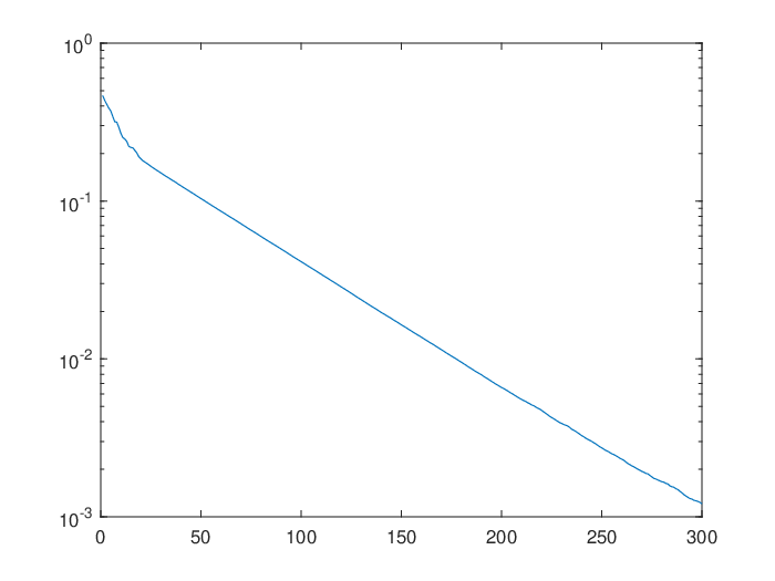
In Figure 3, we performed $600$ iterations of the same quadratic used in this section with $\mu=1,L=200$ . Noting that we can converge no closer to the optimum than the truncation error, we set $m_{k}=91$ for the fixed level algorithm. This is the largest amount of basis functions we reach in the UQ algorithm run under these parameters. At this level, the truncation error is approximately $1.6\times 10^{-5}$ . In each case, we took $250$ Monte Carlo samples to calculate integrals. We note this implies that in the fixed level case $C_{G}=1+2Q_{91}/M_{k}\leq 1+182/250=1.728$ .

At this level, the truncation error is approximately $7.1\times 10^{-7}$ . The following graph gives the averaged results over $200$ trials. We see that the UQ method has outperformed the fixed level variant due to being able to take advantage of larger stepsizes.

Furthermore, not only has the UQ method outperformed the fixed level algorithm in terms of convergence, it has also greatly outperformed it in terms of performance. Each trial of the UQ method took approximately $2.5$ seconds, and each trial of the fixed level method took approximately $4$ seconds. So not only do we converge faster with UQ, we also do it in less time. If we compare the convergence of both methods where we allot the same amount of computational time to each, we see that the UQ method converges about two orders of magnitude more than when we keep the basis functions fixed.

7 Conclusion

In this paper we introduced a gradient descent and accelerated gradient descent equivalent to the stochastic uncertainty quantification method given by [5]. We motivated our method by considering that to estimate the statistics of $x^{*}(\theta)$ naively, we would need to perform gradient descent an exponential number of times.

We showed that each method converges linearly to a solution, and as the number of basis functions grows, we eventually converge to a $\varepsilon$ neighborhood of the true solution. Numerical evidence supported the above claims for each method.

For our purposes we assumed that $f$ must be strongly convex for each $\theta$ . It would be interesting to know how much these properties can be weakened to still obtain useful results on the basis vectors $u$ . Similarly, we hope to subsequently analyse the utility of this method on various industrial applications.

References

[1] N. S. Aybat, A. Fallah, M. Gurbuzbalaban, and A. Ozdaglar, A universally optimal multistage accelerated stochastic gradient method, in Advances in Neural Information Processing Systems, 2019, pp. 8525–8536.
[2] N. S. Aybat, A. Fallah, M. Gurbuzbalaban, and A. Ozdaglar, Robust accelerated gradient methods for smooth strongly convex functions, SIAM Journal on Optimization, 30 (2020), pp. 717–751.
[3] C. Canuto, M. Y. Hussaini, A. Quarteroni, and T. A. Zang, Spectral methods, Springer, 2006.
[4] X. Chen and H. White, Asymptotic properties of some projection-based robbins-monro procedures in a hilbert space, Studies in Nonlinear Dynamics & Econometrics, 6 (2002).
[5] S. Crépey, G. Fort, E. Gobet, and U. Stazhynski, Uncertainty quantification for stochastic approximation limits using chaos expansion, SIAM/ASA Journal on Uncertainty Quantification, 8 (2020), pp. 1061–1089.
[6] S. Hochreiter, A. S. Younger, and P. R. Conwell, Learning to learn using gradient descent, in International Conference on Artificial Neural Networks, Springer, 2001, pp. 87–94.
[7] Z. Hu and S. Mahadevan, Uncertainty quantification and management in additive manufacturing: current status, needs, and opportunities, The International Journal of Advanced Manufacturing Technology, 93 (2017), pp. 2855–2874.
[8] A. A. Kulkarni and V. S. Borkar, Finite dimensional approximation and newton-based algorithm for stochastic approximation in hilbert space, Automatica, 45 (2009), pp. 2815–2822.
[9] R. Nixdorf, An invariance principle for a finite dimensional stochastic approximation method in a hilbert space, Journal of Multivariate Analysis, 15 (1984), pp. 252–260.
[10] F. Papi, L. Cappugi, S. Salvadori, M. Carnevale, and A. Bianchini, Uncertainty quantification of the effects of blade damage on the actual energy production of modern wind turbines, Energies, 13 (2020), p. 3785.
[11] H. Robbins and S. Monro, A stochastic approximation method, The annals of mathematical statistics, (1951), pp. 400–407.
[12] T. J. Sullivan, Introduction to uncertainty quantification, vol. 63, Springer, 2015.
[13] B. Van Scoy, R. A. Freeman, and K. M. Lynch, The fastest known globally convergent first-order method for minimizing strongly convex functions, IEEE Control Systems Letters, 2 (2017), pp. 49–54.
[14] X. Wang, Method of steepest descent and its applications, IEEE Microwave and Wireless Components Letters, 12 (2008), pp. 24–26.
[15] G. Yin, On h–valued stochastic approximation: finite dimenstional projections, Stochastic Analysis and Applications, 10 (1992), pp. 363–377.
[16] G. Yin and Y. Zhu, On h-valued robbins-monro processes, Journal of multivariate analysis, 34 (1990), pp. 116–140.
[17] L. Zhao, W.-Z. Song, and X. Ye, Fast decentralized gradient descent method and applications to in-situ seismic tomography, in 2015 IEEE International Conference on Big Data (Big Data), IEEE, 2015, pp. 908–917.

Appendix A Strong Convexity Properties

In this appendix, we give many typical properties of strongly convex functions and show that they still hold under our definition of strong convexity. We recall again that definition:

Definition 28.

Consider a function $f:L^{2}_{\pi}\times\mathbb{R}^{d}\rightarrow\mathbb{R}$ . We say that $f$ is strongly convex with parameter $\mu$ if:

\langle\nabla f(x_{1}(\theta),\theta)-\nabla f(x_{2}(\theta),\theta),x_{1}(\theta)-x_{2}(\theta)\rangle_{\pi}\geq\mu||x_{1}(\theta)-x_{2}(\theta)||_{\pi}^{2}

(40)

for all $x_{1}(\cdot),x_{2}(\cdot)\in L^{2}_{\pi}$ .

Similarly, we can give an equivalent definition for convexity:

Definition 29.

Consider a function $f:L^{2}_{\pi}\times\mathbb{R}^{d}\rightarrow\mathbb{R}$ . We say that $f$ is convex if:

\langle\nabla f(x_{1}(\theta),\theta)-\nabla f(x_{2}(\theta),\theta),x_{1}(\theta)-x_{2}(\theta)\rangle_{\pi}\geq 0

(41)

for all $x_{1}(\cdot),x_{2}(\cdot)\in L^{2}_{\pi}$ .

We also define a quantity that will be useful going forward:

Definition 30.

Let $f(x(\theta),\theta)$ be some function evaluated at $x(\theta)$ . Then we define the mean of $f$ at $x(\theta)$ as:

M(f(x(\theta),\theta))\vcentcolon=\langle f(x(\theta),\theta),1\rangle_{\pi}=\mathbb{E}_{\pi}\left(f(x(\theta,\theta)\right)\int_{\Theta}f(x(\theta),\theta)\pi d(\theta).

(42)

The main results we want to prove is the following:

Lemma 31.

Let $f$ be a convex function as per Definition 28, and let $\nabla f$ be Lipschitz continuous with parameter $L$ Then we have:

M\left(f(y(\theta),\theta)\right)\leq M\left(f(x(\theta),\theta)\right)+\langle\nabla f(x(\theta)),y(\theta)-x(\theta)\rangle_{\pi}+\frac{L}{2}||y(\theta)-x(\theta)||_{\pi}^{2}

Proof.

Consider the uni-variate function $g(t)$ such that:

g(t)=f(x(\theta)+t(y(\theta)-x(\theta)),\theta)

for some arbitrary $x(\theta),y(\theta)$ . We then see:

g^{\prime}(t)-g^{\prime}(0)=\langle\nabla f(x(\theta)+t(y(\theta)-x(\theta)),\theta)-\nabla f(x(\theta),\theta),y(\theta)-x(\theta)\rangle_{2},

(43)

where we note the norm in this case is the $2$ -norm. Here we are treated $\theta$ as fixed and taking the $2$ -norm between the real numbers we get assuming a fixed $\theta$ . From this expression, we can integrate to find:

M\left(f(y(\theta),\theta)\right)=M\left(g(1)\right)\leq M\left(g(0)\right)+M\left(\int_{t=0}^{1}g^{\prime}(t)dt\right)

Next, note that Fubini’s Theorem holds here so we can swap the order of integration to find:

		$\displaystyle M\left(\int_{t=0}^{1}g^{\prime}(t)dt\right)$
		$\displaystyle=\int_{t=0}^{1}M\left(g^{\prime}(t)\right)dt$
		$\displaystyle\leq\int_{t=0}^{1}\langle\nabla f(x(\theta)+t(y(\theta)-x(\theta)),\theta)-\nabla f(x(\theta),\theta),y(\theta)-x(\theta)\rangle_{\pi}+M\left(f(x(\theta),\theta)\right)dt$
		$\displaystyle\leq M\left(f(x(\theta),\theta)\right)+\int_{t=0}^{1}\frac{L}{2}\|\|y(\theta)-x(\theta)\|\|_{\pi}$

where we have used the fact that $g^{\prime}(t)=g^{\prime}(t)-g^{\prime}(0)+g^{\prime}(0)$ , along with Equation (43) and Lipschitz Continuity. Now substituting our expressions for $g$ , we find:

M\left(f(y(\theta),\theta)\right)\leq M\left(f(x(\theta),\theta)\right)+\langle\nabla f(x(\theta)),y(\theta)-x(\theta)\rangle_{\pi}+\frac{L}{2}||y(\theta)-x(\theta)||_{\pi}^{2}

Due to this modified form of the standard quadratic upper bound, we can now say:

Lemma 32.

Let $f$ be a convex function as per Definition 28, and let $\nabla f$ be Lipschitz continuous with parameter $L$ Then we have:

M\left(f(x(\theta),\theta)-f(x^{*}(\theta),\theta)\right)\geq\frac{1}{2L}||\nabla f(x(\theta))||_{\pi}^{2}

Proof.

We seek to minimise the upper bound we found in the previous Lemma in $y$ :

M\left(f(y(\theta),\theta)\right)\leq M\left(f(x(\theta),\theta)\right)+\langle\nabla f(x(\theta)),y(\theta)-x(\theta)\rangle_{\pi}+\frac{L}{2}||y(\theta)-x(\theta)||_{\pi}^{2}

We first note that $y(\theta)-x(\theta)$ being parallel to $-\nabla f(x(\theta)$ will minimise the upper bound, so letting $y(\theta)-x(\theta)=-c\nabla f(x(\theta))$ we get:

M\left(f(y(\theta),\theta)\right)\leq M\left(f(x(\theta),\theta)\right)+\frac{Lc^{2}-2c}{2}||\nabla f(x(\theta))||_{\pi}^{2}

from which we find this is minimised when $c=-1/L$ , and thus find:

\inf_{y}M\left(f(y(\theta),\theta)\right)=M\left(f(x^{*}(\theta),\theta)\right)\leq M\left(f(x(\theta),\theta)\right)-\frac{1}{2L}||\nabla f(x(\theta),\theta)||_{\pi}^{2},

where we reach our conclusion upon rearranging.

From this Lemma, we can prove our first main result, an adaption of co-coercivity of the gradient:

Theorem 33.

Let $f$ be convex and have Lipschitz gradient with parameter $L$ . Then:

\langle\nabla f(x(\theta),\theta)-\nabla f(y(\theta),\theta),x(\theta)-y(\theta)\rangle_{\pi}\geq\frac{1}{L}||\nabla f(x(\theta),\theta)-\nabla f(y(\theta),\theta)||_{\pi}^{2}

Proof.

Define the following two functions:

f_{x}(z(\theta),\theta)=f(z(\theta),\theta)-\langle\nabla f(x(\theta),\theta),z(\theta)\rangle_{2},\qquad f_{y}(z(\theta),\theta)=f(z(\theta),\theta)-\langle\nabla f(y(\theta),\theta),z(\theta)\rangle_{2}

where again, we note that we use the $2$ -norm, as we are again treating $\theta$ as fixed and taking the $2$ -norm between the real numbers we get assuming a fixed $\theta$ .

We note that $z(\theta)=x(\theta)$ is the minimiser of $f_{x}(z)$ , and so we can write:

		$\displaystyle M\left(f(y(\theta),\theta)-f(x(\theta),\theta)-\langle\nabla f(x(\theta),\theta),y(\theta)-x(\theta)\right)$
		$\displaystyle=M\left(f_{x}(y(\theta),\theta)-f_{x}(x(\theta),\theta)\right)$
		$\displaystyle\geq\frac{1}{2L}\|\|\nabla f_{x}(x(\theta),\theta)\|\|_{\pi}=\frac{1}{2L}\|\|\nabla f(y(\theta),\theta)-\nabla f(x(\theta),\theta)\|\|_{\pi}$

using Lemma 32. Similarly, we can show using $f_{y}$ :

M\left(f(x(\theta),\theta)-f(y(\theta),\theta)-\langle\nabla f(y(\theta),\theta),x(\theta)-y(\theta)\right)\geq\frac{1}{2L}||\nabla f(y(\theta),\theta)-\nabla f(x(\theta),\theta)||_{\pi}

and adding these two Equations gives the result.

We can also, like in the usual case, extend co-coercivity to strongly convex functions as follows:

Theorem 34.

Suppose $f$ is a strongly convex function with strong convexity parameter $\mu$ , and has Lipschitz gradient with parameter $L$ . Then we have:

		$\displaystyle(L+\mu)\langle\nabla f(x(\theta),\theta)-\nabla f(y(\theta)),x(\theta)-y(\theta)\rangle_{\pi}$
		$\displaystyle\geq\mu L\|\|x(\theta)-y(\theta)\|\|_{\pi}^{2}+\|\|\nabla f(x(\theta),\theta)-\nabla f(y(\theta),\theta)\|\|_{\pi}^{2}$

Proof.

This result follows in a standard way: we note the function:

h(x(\theta),\theta)=f(x(\theta),\theta)-\mu||x(\theta)||_{2}^{2}

where again, we use the $2$ -norm, and treat $\theta$ as fixed. It is clear this function is convex and $(L-\mu)$ smooth, and so applying Theorem 33 to $h$ gives the result.

Appendix B Accelerated Gradient Descent Lemmas

The goal of this section is to prove Lemma 21, which we state again here:

Lemma 35.

Under all our usual hypotheses, and that there exists $\rho\in(0,1)$ and $\tilde{P}\in\mathbb{S}_{+}^{2}$ , possibly depending on $\rho$ such that:

\rho^{2}\tilde{X_{1}}+(1-\rho^{2})\tilde{X_{2}}\succeq\begin{pmatrix}A^{T}PA-\rho^{2}P&A^{T}PB\\ B^{T}PA&B^{T}PB\end{pmatrix}

where:

\tilde{X_{1}}=\frac{1}{2}\begin{pmatrix}\beta^{2}\mu&-\beta^{2}\mu&-\beta\\ -\beta^{2}\mu&\beta^{2}\mu&\beta\\ -\beta&\beta&\alpha(2-L\alpha)\end{pmatrix}

and:

\tilde{X_{2}}=\frac{1}{2}\begin{pmatrix}(1+\beta)^{2}\mu&-\beta(1+\beta)\mu&-(1+\beta)\\ -\beta(1+\beta)\mu&\beta^{2}\mu&\beta\\ -(1+\beta)&\beta&\alpha(2-L\alpha)\end{pmatrix}.

Then let $P=\tilde{P}\otimes I_{d}$ . We have for all $k\geq 0$ :

\mathbb{E}(V_{P}(\xi_{k+1})|\mathcal{F}_{k+1})\leq\rho^{2}\mathbb{E}(V_{P}(\xi_{k})|\mathcal{F}_{k})+\alpha^{2}\left(C+C_{G}\mathbb{E}\left(||y^{k}-x^{*}||_{\pi}^{2}|\mathcal{F}_{k}\right)\right)\left(\frac{L}{2}+\tilde{P}_{11}\right)

Throughout this section, we will find it useful to revisit our defining inequality for strong convexity:

\langle\nabla f(x_{1}(\theta),\theta)-\nabla f(x_{2}(\theta),\theta),x_{1}(\theta)-x_{2}(\theta)\rangle_{\pi}\geq\mu||x_{1}(\theta)-x_{2}(\theta)||_{\pi}^{2}

(44)

And we note that as $x^{*}$ is a minimum, we can add $M\left(f(x_{1}(\theta),\theta)-\pi f(x^{*}(\theta),\theta\right)$ to the left hand side of this inequality, where we use $x_{2}=x^{*}$ . Rearranging, we find:

$\displaystyle M\left(f(x_{1}(\theta),\theta)\right)$		(45)
	$\displaystyle\geq M\left(f(x^{*}(\theta),\theta)\right)+\langle\nabla f(x_{1}(\theta),\theta)-\nabla f(x_{2}(\theta),\theta),x_{1}(\theta)-x_{2}(\theta)\rangle_{\pi}$
	$\displaystyle+\mu\|\|x_{1}(\theta)-x_{2}(\theta)\|\|_{\pi}^{2}.$

Due to the similarity with the usual inequality for strong convexity (apart from the expectation taken), we will refer to this as using the strong convexity inequality in expectation.

Before we begin the proof, we must prove a couple of preliminary Lemmas, adapted from [1]. Firstly:

Lemma 36.

Consider the function $W_{P}(\xi)=(\xi-\xi^{*})^{T}P(\xi-\xi^{*})$ . Let $P=\tilde{P}\otimes I_{d}$ , where $\tilde{P}\in\mathbb{S}_{+}^{2}$ . Then we have:

	$\displaystyle\mathbb{E}(W_{P}(\xi_{k+1})\|\mathcal{F}_{k+1})\leq$	$\displaystyle\mathbb{E}\left[\begin{pmatrix}\xi_{k}-\xi^{}\\ \tilde{\nabla g(y^{k})}\end{pmatrix}\begin{pmatrix}A^{T}PA&A^{T}PB\\ B^{T}PA&B^{T}PB\end{pmatrix}\begin{pmatrix}\xi_{k}-\xi^{}\\ \tilde{\nabla g(y^{k})}\end{pmatrix}\|\mathcal{F}_{k}\right]$
		$\displaystyle+\left(C_{G}\mathbb{E}\left(\|\|y^{k}-x^{*}\|\|_{\pi}\|\mathcal{F}_{k}^{2}\right)+C\right)\alpha^{2}\tilde{P}_{11}$

Proof.

Virtually identical to [1], other than we use our noise model from Equation (27).

Secondly, by following Lemma $4.5$ in [2], we can get:

Lemma 37.

Consider a strongly convex $f$ for each $\theta$ , and consider the dynamical system representation of AG. Then, for any $\rho\in(0,1)$ :

		$\displaystyle\mathbb{E}\left[\begin{pmatrix}\xi_{k}-\xi^{}\\ \tilde{\nabla g(y^{k})}\end{pmatrix}\left(\rho^{2}X_{1}+(1-\rho^{2})X_{2}\right)\begin{pmatrix}\xi_{k}-\xi^{}\\ \tilde{\nabla g(y^{k})}\end{pmatrix}\|\mathcal{F}_{k+1}\right]$
		$\displaystyle\leq\rho^{2}\mathbb{E}h(x^{k}(\theta)\|\mathcal{F}_{k})-\mathbb{E}h(x^{k+1}(\theta)\|\mathcal{F}_{k+1})+\frac{L\alpha^{2}}{2}\left(C_{G}\mathbb{E}\left(\|\|y^{k}-x^{*}\|\|_{\pi}^{2}\|\mathcal{F}_{k}\right)+C\right)$

where as previously defined, $h(x(\theta))=M\left(f(x(\theta),\theta))-f(x^{*}(\theta),\theta)\right)$ .

Proof.

Identical to [2], except in place of Equations $4.19-4.20$ , we use the strong convexity inequality in expectation with respect to $\pi$ .

With these two Lemmas, we can now give our proof:

Proof of Lemma 21.

By the definition of $V_{P}$ we can expand in the following way:

	$\displaystyle V_{P}(\xi_{k+1})-\rho^{2}V_{P}(\xi_{k})$	$\displaystyle=$
		$\displaystyle=W_{P}(\xi_{k+1})-\rho^{2}W_{P}(\xi_{k})+h(\xi_{k+1})-\rho^{2}h(\xi_{k})$

then on taking expectations, we can use the previous two Lemmas, along with the hypothesis on the matrix $\rho^{2}\tilde{X_{1}}+(1-\rho^{2})\tilde{X_{2}}$ to see:

		$\displaystyle\mathbb{E}\left(V_{P}(\xi_{k+1})\|\mathcal{F}_{k+1}\right)-\rho^{2}\mathbb{E}\left(V_{P}(\xi_{k})\|\mathcal{F}_{k}\right)$
		$\displaystyle=\mathbb{E}\left(W_{P}(\xi_{k+1}\|\mathcal{F}_{k+1})\right)-\rho^{2}\mathbb{E}\left(W_{P}(\xi_{k})\|\mathcal{F}_{k}\right)+\mathbb{E}h(\xi_{k+1}\|\mathcal{F}_{k+1})-\rho^{2}\mathbb{E}h(\xi_{k}\|\mathcal{F}_{k})$

which leads to:

	$\displaystyle\mathbb{E}\left(W_{P}(\xi_{k+1})-W_{P}(\xi_{k})\|\mathcal{F}_{k+1}\right)+$	$\displaystyle\mathbb{E}\left(h(\xi_{k+1})-\rho^{2}h(\xi_{k})\|\mathcal{F}_{k+1}\right)\leq$
		$\displaystyle\leq\mathbb{E}\left(\rho^{2}h(\xi^{k})-h(\xi^{k+1})+h(\xi^{k+1})-\rho^{2}h(\xi^{k})\|\mathcal{F}_{k+1}\right)$
		$\displaystyle+\left(\frac{L\alpha^{2}}{2}+\alpha^{2}\tilde{P}_{11}\right)\left(C_{G}\mathbb{E}\left(\|\|y^{k}-x^{*}\|\|_{\pi}^{2}\|\mathcal{F}_{k}\right)+C)\right)$
		$\displaystyle=\left(\frac{L\alpha^{2}}{2}+\alpha^{2}\tilde{P}_{11}\right)\left(C_{G}\mathbb{E}\left(\|\|y^{k}-x^{*}\|\|_{\pi}^{2}\|\mathcal{F}_{k}\right)+C)\right)$
		$\displaystyle=\alpha^{2}\left(C_{G}\mathbb{E}\left(\|\|y^{k}-x^{*}\|\|_{\pi}^{2}\|\mathcal{F}_{k}\right)+C)\right)\left(\frac{L}{2}+\tilde{P}_{11}\right)$

from which the statement follows.

	$\displaystyle\mathbb{E}(\|\|e_{k}\|\|_{2}^{2}\|$	$\displaystyle\mathcal{F}_{k-1})$
		$\displaystyle=\sum_{i=1}^{m_{k}}\mathbb{E}(e_{i,k}^{2}\|\mathcal{F}_{k-1})$
		$\displaystyle=\sum_{i=1}^{m_{k}}\mathbb{E}\left(\left(\frac{1}{M_{k}}\sum_{j=1}^{M_{k}}\nabla F(x^{k}(\theta_{j}),\theta_{j},v_{j})B_{i}(\theta_{j})B_{i}(\theta_{j})-\int\nabla f(x^{k}(\theta),\theta)B_{i}(\theta)\pi(d\theta)\right)^{2}\|\mathcal{F}_{k-1}\right)$
		$\displaystyle\leq\frac{Q_{m_{k}}}{M_{k}}\left(V_{G}\|\|\nabla f(x^{k}(\theta),\theta)\|\|_{\pi}^{2}+V\right)$

$\displaystyle\mathbb{E}(e_{i,k}^{2}\|\mathcal{F}_{k-1},\Theta_{k})$
	$\displaystyle=\mathbb{E}\left(\left(a_{i,k}+b_{i,k}\right)^{2}\|\mathcal{F}_{k-1},\Theta_{k}\right)$
	$\displaystyle=\mathbb{E}\left(a_{i,k}^{2}\|\mathcal{F}_{k-1},\Theta_{k}\right)+\mathbb{E}\left(b_{i,k}^{2}\|\mathcal{F}_{k-1},\Theta_{k}\right),$	(18)

	$\displaystyle\mathbb{E}(d_{k+1}^{2}\|\mathcal{F}_{k})$
		$\displaystyle\leq\mathbb{E}(d_{k}^{2}\|\mathcal{F}_{k-1})-2\gamma\frac{\mu L}{\mu+L}\mathbb{E}(d_{k}^{2}\|\mathcal{F}_{k-1})+\gamma^{2}C$
		$\displaystyle+\gamma\left(\gamma C_{G}-\frac{2}{\mu+L}\right)\mathbb{E}\left(\|\|\nabla f(x(\theta),\theta)-\nabla f(x_{m_{k}}^{*}(\theta),\theta)\|\|_{2}^{2}\|\mathcal{F}_{k-1}\right)$
		$\displaystyle\leq\left(1-\frac{2\gamma\mu L}{\mu+L}\right)\mathbb{E}(d_{k}^{2}\|\mathcal{F}_{k-1})+\gamma^{2}C$

		$\displaystyle\mathbb{E}\left(\|\|u^{k+1}-u^{*}\|\|_{2}\right)$
		$\displaystyle\leq\mathbb{E}\|\|u^{k+1}-u^{}_{k}\|\|_{2}+\|\|u^{}-u^{*}_{k}\|\|_{2}$
		$\displaystyle\leq\left(1-\frac{2\gamma\mu L}{\mu+L}\right)^{1/2}\left(\mathbb{E}\|\|u^{k}-u^{*}_{k}\|\|_{2}\right)+\varepsilon+\sqrt{\varepsilon}$
		$\displaystyle\leq\left(1-\frac{2\gamma\mu L}{\mu+L}\right)^{1/2}\left(\mathbb{E}\|\|u^{k}-u^{}\|\|_{2}+\|\|u^{}-u^{*}_{k}\|\|_{2}\right)+\varepsilon+\sqrt{\varepsilon}$
		$\displaystyle\leq\left(1-\frac{2\gamma\mu L}{\mu+L}\right)^{1/2}\left(\mathbb{E}\|\|u^{k}-u^{*}\|\|_{2}\right)+2\varepsilon+\sqrt{\varepsilon}$

	$\displaystyle\mathbb{E}(V_{P_{\alpha}}(\xi_{k+1})\|\mathcal{F}_{k+1})$	$\displaystyle\leq\left(1-\sqrt{\alpha\mu}\right)\mathbb{E}(V_{P_{\alpha}}(\xi_{k})\|\mathcal{F}_{k})$
		$\displaystyle+\frac{1}{2}\mathbb{E}\left((\xi^{k}-\xi^{})^{T}2\alpha c^{2}C^{T}C(\xi^{k}-\xi^{})\|\mathcal{F}_{k+1}\right)+\alpha C$
		$\displaystyle\leq\left(1-\sqrt{\alpha\mu}\right)\mathbb{E}(V_{Q_{\alpha}}(\xi_{k})\|\mathcal{F}_{k})+\alpha C$