Weighted Quantum Channel Compiling through Proximal Policy Optimization
Abstract
We propose a general and systematic strategy to compile arbitrary quantum channels without using ancillary qubits, based on proximal policy optimization—a powerful deep reinforcement learning algorithm. We rigorously prove that, in sharp contrast to the case of compiling unitary gates, it is impossible to compile an arbitrary channel to arbitrary precision with any given finite elementary channel set, regardless of the length of the decomposition sequence. However, for a fixed accuracy one can construct a universal set with constant number of -dependent elementary channels, such that an arbitrary quantum channel can be decomposed into a sequence of these elementary channels followed by a unitary gate, with the sequence length bounded by . Through a concrete example concerning topological compiling of Majorana fermions, we show that our proposed algorithm can conveniently and effectively reduce the use of expensive elementary gates through adding the weighted cost into the reward function of the proximal policy optimization.
Quantum compilers, which decompose quantum operations into hardware compatible elementary operations, play an important role in quantum computation Nielsen and Chuang 2010 and digital simulation Georgescu et al. 2014. This technique is especially crucial for the applications of noisy intermediate-scale quantum devices Preskill 2018, where the performance of deep quantum circuits might be limited by noises and quantum decoherences. A number of notable approaches have been proposed to compile unitary gates and the dynamics of isolated quantum systems Dawson and Nielsen 2005; Kitaev et al. 2002; Jones et al. 2012; Fowler 2011; Bocharov and Svore 2012; Bocharov et al. 2013; Pham et al. 2013; Zhiyenbayev et al. 2018; Kliuchnikov et al. 2013; Selinger 2013; Gosset et al. 2014; Ross and Selinger 2016; Heyfron and Campbell 2018. However, in reality quantum systems cannot be perfectly isolated and would inevitably interact with the external environment, making the more general quantum channel compiling indispensable for a wide range of applications Breuer et al. 2002; Lidar 2019.Yet, quantum channel compilation has been barely explored Braun et al. 2014, with major previous attention paid to exploiting the Stinespring dilation theorem Stinespring 1955 and compiling arbitrary quantum channels through elementary gates acting on an expanded Hilbert space with ancillary qubits playing an prerequisite role Wang et al. 2013; Iten et al. 2017; Wei et al. 2018; Iten et al. 2016; Shen et al. 2017; Sweke et al. 2014; Passos et al. 2020; Wang and Sanders 2015; Lu et al. 2017; Xin et al. 2017. Hitherto, a general and systematic strategy to compile arbitrary quantum channels without using ancillary qubits has not been established. Here, we prove two generic theorems regarding channel compiling and introduce such a strategy based on deep reinforcement learning (see Fig. 1 for an illustration).
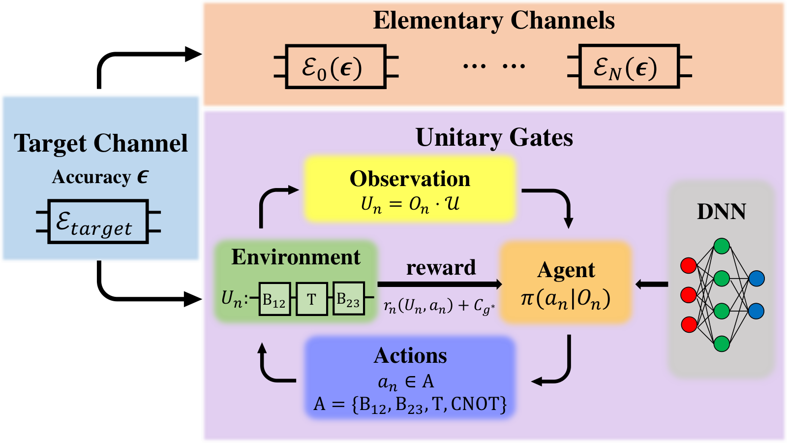
Machine learning, or more broadly artificial intelligence, has recently cracked a number of notoriously challenging problems, such as playing the game of Go Silver et al. 2016; Silver et al. 2017, predicting protein spatial structures Senior et al. 2020, and weather forecasting Ravuri et al. 2021. Its tools and techniques have been broadly exploited in various quantum physics tasks, including representing quantum many-body states Carleo and Troyer 2017; Gao et al. 2017, quantum state tomography Torlai et al. 2018; Carrasquilla et al. 2019, learning topological phases of matter Zhang and Kim 2017; Carrasquilla and Melko 2017; van Nieuwenburg et al. 2017; Wang 2016; Broecker et al. 2017; Ch’ng et al. 2017; Zhang et al. 2017; Wetzel 2017; Hu et al. 2017; Zhang et al. 2019; Lian et al. 2019, and nonlocality detection Deng 2018. For quantum compiling on unitary gates, machine learning approaches have also been introduced to provide a near-optimal sequence Alam 2019; Zhang et al. 2020. In this paper, we first rigorously prove that it is impossible to compile any quantum channel to arbitrary accuracy using unitary gates and a finite set of elementary channels, which is in sharp contrast to the case of compiling a unitary gate. As illustrated in Fig. 1, we propose a quantum channel compiler which given an accuracy demand , decomposes any quantum channel into a sequence of finite types of elementary quantum channels followed by a unitary gate. We provide a constructive method to obtain the elementary channel set and show that the size of the set scales as with the dimension of Hilbert space and is independent of . We additionally prove that the length of the elementary channel sequence in the decomposition is bounded above by . For the unitary gate at the end of the decomposition, we train a deep reinforcement learning (DRL) agent to decompose it into hardware compatible elementary gates. To reduce the resource requirement of the compiler, we exploit the proximal policy optimization (PPO) algorithm Schulman et al. 2017 to train our agent with weighted cost in the reward function to reduce the use of experimentally-expensive elementary gates. We further prove a lower bound for any indispensable expensive elementary gate count to compile an arbitrary unitary gate within error . As a benchmark, we apply our algorithm to the topological quantum compiling of Majorana fermions Kitaev 2006; Nayak et al. 2008, whose braidings together with a non-topological gate form a universal set. We numerically show that our algorithm could reduce the use of gate by a factor of two compared to the traditional Solovay-Kitaev algorithm.
Notations.—To begin with, we first introduce some basic notations and concepts Nielsen and Chuang 2010. A quantum state can be represented by a positive semi-definite operator with , where is the Hilbert space and the set of operators on . In general, a quantum channel can be characterized by a completely positive, trace-preserving (CPTP) map which maps a quantum state into another state . Any single-qubit state can be represented as , where is a three-dimensional vector within the Bloch sphere and are Pauli matrices. Any linear CPTP map for a single-qubit system could be represented by a four-by-four matrix Ruskai et al. 2002; Wolf and Cirac 2008; Wang et al. 2013; Wang 2015:
| (1) |
where , represents the Pauli matrix and . Under this representation, a channel is an affine map King and Ruskai 2001 . Geometrically, maps the states within the Bloch sphere into states enveloped by an ellipsoid, with the center shift from the original center and the distortion matrix for the ellipsoid. When , the CPTP map reduces to a unitary gate. In this sense, unitary gates can be regarded as special channels. Throughout this paper, we differentiate unitary gates from channels for clarity.
A general theorem for channel compilation.—To formulate the problem, we consider a set with metric . A set is called a -net if for any , there exists such that Kitaev et al. 2002. The subset is called a dense subset under metric if it is a -net of for arbitrary .
Suppose we have a set of elementary channels and want to approximate the target channel with a sequence of unitary gates and elementary channels chosen from the set. For technical convenience and simplicity, we consider Schatten one-norm Kliesch et al. 2011 as the distance measure. Now, we are ready to present our general theorem.
Theorem 1. Consider compiling single-qubit channels using unitary gates and elementary channels with Schatten one-norm as the distance measure. Then:
(1) Given a finite set of elementary channels together with an arbitrary unitary gate, it is impossible to compile an arbitrary single-qubit channel to arbitrary accuracy.
(2) Given an accuracy bound , one can construct a finite set of elementary quantum channels using as a parameter such that any single-qubit channel can be compiled by the elementary channels from this set and a unitary gate within error . The length of sequence is bounded above by .
proof. We provide the main idea here. The full proof is technically involved and thus left to the Supplementary Materials sup. Suppose that we are provided with a finite set of elementary channels with corresponding distortion matrices and center shifts . Without loss of generality, we assume that . Noting that the composition of channels could not increase the determinant of the distortion matrix, thus a target channel with cannot be compiled by the channels chosen from to arbitrary accuracy, independent of how long the decomposition sequence is. For part (2), we decompose the compiling process into several steps and provide a constructive proof. For a target channel with distortion matrix with eigenvalues and center shift , we first implement intermediate channel with parameters using elementary channels parametrized by . We then use a unitary gate to realize the negative, complex eigenvalues and basis transformations.
The above theorem could be extended to multi-qubit channels. For a -dimensional quantum state , there exists a canonical and orthonormal basis Wang 2015; Brüning et al. 2012. A density operator under such basis could be written as . The parameters in form the polarization vector of a -dimensional ball with representing pure states and representing mixed states. As a quantum state can be represented by a vector within a ball, a quantum channel can be written as an affine map represented by distortion matrix and center shift similar to Eq. (1). With this representation, we can extend the Theorem 1 to the multi-qubit case sup. Yet, it is worthwhile to mention that in this case, the size of set of constructed quantum channels should scale as in part (2) of the theorem sup.
The above results imply that a finite number of elementary channels could not approximate an arbitrary target channel to arbitrary accuracy, regardless of the specific structure of each elementary channel and the length of the compiling sequence. This is in sharp contrast with the case of unitary gate compiling, where we can use a small number of elementary gates to compile an arbitrary unitary gate within any accuracy demand. We remark that any quantum channel can be implemented by a sequence of elementary unitary gates acting on a dilated Hilbert space and this seems to contradict with the claim of part (1) in the Theorem 1. However, this spurious contradiction dissolves after noting the fact that tracing out the ancillary qubits at different sequence locations would effectively result in different channels even for the same elementary unitary gates. In other words, although a small number of different unitary gates suffice to implement any quantum channel with ancillary qubits, when restricted to the targeted system no finite set of elementary channels is universal.
In the proof for part (2) of the Theorem 1, we have provided two explicit constructions to decompose an arbitrary quantum channel into a sequence of elementary channels followed by a unitary gate sup. The first construction has an elementary channel set of size with a sequence length , and the other uses a much larger elementary channel set [of size ] but much shorter decomposition sequence [of length ]. In other words, we can decompose any target quantum channel into a fixed sequence of elementary channels followed by a -qubit unitary gate. The channel compilation task has thus been reduced to unitary compiling with elementary unitary gates.
Weighted unitary gate compilation and a DRL algorithm.—We now consider quantum compilation for unitary gates with the elementary gate set . A gate set is universal if it can compile arbitrary unitary gates to any given accuracy demand under the distance measure. In other words, a gate set is universal if and only if it generates a dense subgroup in Kitaev et al. 2002. We present the following theorem concerning the lower bound of any indispensable gate in compiling an arbitrary unitary.
Theorem 2. For a non-dense subgroup generated by , suppose we can find such that generated by is dense in . When employing as elementary gate set for quantum compilation task on , the number of gate to compile an arbitrary gate within distance is bounded below by:
| (2) |
The proof of Theorem 2 relies on the volume method, which considers covering the whole space with -balls centered at each possible gate sequence. For brevity, we leave the technical details to the Supplementary Materials sup. This theorem gives a lower bound for the count of any indispensable gate in compiling an arbitrary unitary, which scales linearly in but quadratic in the Hilbert space dimension that is exponentially large as the system size increases. In practical applications, may represent some experimentally expensive or flawed gate and thus reducing its count in compiling could be crucial. For the case of quantum compiling with Clifford gate set, a number of striking algorithms Kliuchnikov et al. 2013; Selinger 2013; Gosset et al. 2014; Ross and Selinger 2016; Heyfron and Campbell 2018, which either exploit its specific structures or utilize ancillary qubits, have been proposed to reduce the count. Here, we introduce a more general approach (in the sense that it does not rely on the special properties of the elementary gate set and thus bears universal applicability) without using ancillary qubits. We exploit a reinforcement learning technique, the proximal policy optimization Schulman et al. 2017 in particular, to reduce the count of experimentally expensive gates.
Unlike commonly used Q-learning algorithms Watkins and Dayan 1992; Zhang et al. 2020 such as deep-Q networks Sutton and Barto 2018, PPO directly represents a policy explicitly as by a neural network, which receives the current state as an input and outputs the probability the agent may choose for each action . The updating rules used by PPO explore the biggest possible improvement step without causing a performance collapse Schulman et al. 2017. This property makes PPO particularly suitable for quantum compilation tasks since applying an inappropriate gate in the sequence will dramatically destruct the approximation gate. Moreover, we modify the reward function used in PPO, which efficiently reduces the count of a specific gate that is experimentally costly:
| (3) |
where is the reward that the agent receives for the -th step, is the reward determined by comparing the approximation gate and the target gate , and is the additional weighted punishment for the employment of gates. By increasing , the agent would tend to avoid using gates and thus the count would be reduced in the decomposition sup. By exploiting the PPO algorithm, our algorithm searches the approximation sequence in a depth-first search scheme. Comparing with the breadth-first search DRL algorithm proposed in Ref. Zhang et al. 2020, the PPO algorithm runs with significantly less time and memory in both the training and searching stages. This advantage makes our algorithm feasible for compiling tasks for larger systems with more complicated actions and rewards.
Topological compiling of Majorana fermions. To benchmark the performance of our PPO algorithm in practice, we consider topological compiling with the four-quasiparticle encoding scheme for Majorana fermions Nayak et al. 2008. Two elementary gates corresponding to the braidings of four Majorana fermions are shown in Fig. 2(a) and unitary gates can be approximated through braiding sequences and gates. A simple example for decomposing an -rotation is shown in Fig. 2(b). It is well known that braidings of Majorana fermions only lead to an elementary gate set CNOT, H, S, which is not sufficient for universal quantum computation Bravyi and Kitaev 2005; Nayak et al. 2008. To achieve universality, a non-topological gate with a relatively high experimental cost is necessary. Therefore, reducing count is of practical importance Gheorghiu et al. 2021; Selinger 2015; Matsumoto and Amano 2008. Here, we apply the PPO algorithm to attain this goal. To this end, we note that the topological gate set generates a Clifford group with finite size Calderbank et al. 1998; Nebe et al. 2001; Planat and Jorrand 2008. According to the Theorem 2, the scaling of count for compiling an arbitrary gate in the worst case is .
We mention that topological quantum compiling has been broadly explored with various algorithms proposed Deng et al. 2010; Bonesteel et al. 2005; Xu and Wan 2008; Hormozi et al. 2007; Burrello et al. 2010; Kliuchnikov et al. 2014; Carnahan et al. 2016. Most of the algorithms run in and output sequences of braidings with length to obtain an approximation within distance from given target evolution. Here, we exploit the average gate fidelity provided in the open-source QuTiP package Johansson et al. 2012 to measure the distance between an approximated unitary gate and a target unitary gate . To exploit or DRL algorithm as a single qubit quantum compiler, the action space is a set containing six elementary gates. To train the agent, we employ a deep neural network (DNN) with five layers of fully connected neurons and train it with a PPO algorithm encapsulated in OpenAI gym and baseline package Brockman et al. 2016. To construct the training data, we generate a sequence of length consisting of the elementary gates to be the target gate. To test our agent, we construct a test dataset of data samples, each as a random sequence of gates from of length between and . We compare the performance of our algorithm and the traditional Solovay-Kitaev algorithm on such a dataset sup.

In Fig. 3, we plot the error distribution over the test dataset and the proportion of gate for our algorithm and Solovay-Kitaev algorithm with the same threshold . We observe that the error distributions for both algorithms show two peaks with one below the threshold and the other larger than the threshold. This could be understood as the potential risk of failure for the depth-first search scheme, which is exploited in both algorithms. On average, the Solovay-Kitaev algorithm with net depth provides a more accurate approximation than our algorithm at the price of longer average length while the -depth algorithm provides an equal average length with sacrificed approximation accuracy. In the inset of Fig. 3, we find that by increasing the cost of gate from to , the average gate rate over the test set decreases from to . This is a significant reduction compared to that for the Solovay-Kitaev algorithm which gives a gate rate of . This shows that adding the cost of gate as a punishment in DRL could effectively reduce the count.
We remark that the depth-first search scheme in our PPO algorithm makes the time complexity scale linearly with the maximal search depth . This is distinct from the search (which is breadth-first and hence exhibits an exponential scaling with ) used in Ref. Zhang et al. 2020. As a result, the PPO algorithm is significantly less time and memory consuming in both the training and searching stages. This advantage makes our algorithm feasible for compiling tasks for larger systems with more complicated actions and rewards. As a trade-off, the PPO algorithm would not output the near-optimal sequence for a given target unitary and accuracy demand, and may even fail to find a decomposition if the accuracy threshold is too small. We mention that one can increase the successful rate of the compilation by increasing sup.
Discussion and conclusion.—Theorem 1 implies that for channel compiling, there exists no finite universal elementary channel set. However, for a given target channel, this theorem does not tell whether it can be decomposed into predetermined elementary channels to a desired accuracy. Finding a general and efficiently computable criterion for determining whether a given channel can be compiled with a fixed elementary channel set or not is of both theoretical and experimental importance, and worth future investigation. Another interesting and important future direction is to incorporate a partial breadth-first search mechanism into the current PPO algorithm to increase the success rate and reduce the total length of the output sequences, at the cost of a slightly more time and memory consuming training process. In addition, our proposed PPO algorithm may carry over straightforwardly to other scenarios, including quantum control problems Dong and Petersen 2010 and digital quantum simulations Suzuki 1991; Childs et al. 2021; Berry et al. 2015; Low and Chuang 2019; Bolens and Heyl 2021 for both closed and open systems.
In summary, we have rigorously proved that, in sharp contrast to the case of unitary compiling, it is impossible to compile an arbitrary channel to arbitrary accuracy with any given finite elementary channel set, regardless of the length of the decomposition sequence. We analytically constructed a general scheme to decompose an arbitrary channel into a sequence of elementary channels plus a unitary gate, hence reducing the task of channel compiling to unitary compiling. To reduce the count of certain experimentally expensive gates, we further introduced a DRL algorithm that is generally applicable to any elementary gate set and uses no ancillary qubit. We benchmarked the performance of our algorithm with an example concerning quantum compiling of Majorana fermions, and demonstrated that our approach can reduce the use of expensive gates efficiently and effectively. Our results shed new light on the general problem of quantum compiling, which provides a valuable guide for future studies in both theory and experiment.
Acknowledgement.—We thank Zhengwei Liu, Weikang Li, Yuanhang Zhang, Qi Ye, Xun Gao, and Dong Yuan for helpful discussions. This work was supported by the start-up fund from Tsinghua University (Grant No. 53330300320), the National Natural Science Foundation of China (Grant. No. 12075128), and the Shanghai Qi Zhi Institute.
References
- Nielsen and Chuang (2010) M. A. Nielsen and I. L. Chuang, Quantum Computation and Quantum Information (Cambridge University Press, Cambridge, 2010).
- Georgescu et al. (2014) I. M. Georgescu, S. Ashhab, and F. Nori, “Quantum simulation,” Rev. Mod. Phys. 86, 153 (2014).
- Preskill (2018) J. Preskill, “Quantum computing in the nisq era and beyond,” Quantum 2, 79 (2018).
- Dawson and Nielsen (2005) C. M. Dawson and M. A. Nielsen, “The solovay-kitaev algorithm,” arXiv quant-ph/0505030 (2005).
- Kitaev et al. (2002) A. Y. Kitaev, A. Shen, M. N. Vyalyi, and M. N. Vyalyi, Classical and quantum computation, 47 (American Mathematical Soc., 2002).
- Jones et al. (2012) N. C. Jones, J. D. Whitfield, P. L. McMahon, M.-H. Yung, R. Van Meter, A. Aspuru-Guzik, and Y. Yamamoto, “Faster quantum chemistry simulation on fault-tolerant quantum computers,” New J. Phys. 14, 115023 (2012).
- Fowler (2011) A. G. Fowler, “Constructing arbitrary steane code single logical qubit fault-tolerant gates,” Quantum Inf. Comput. 11, 867 (2011).
- Bocharov and Svore (2012) A. Bocharov and K. M. Svore, “Resource-optimal single-qubit quantum circuits,” Phys. Rev. Lett. 109, 190501 (2012).
- Bocharov et al. (2013) A. Bocharov, Y. Gurevich, and K. M. Svore, “Efficient decomposition of single-qubit gates into v basis circuits,” Phys. Rev. A 88, 012313 (2013).
- Pham et al. (2013) T. T. Pham, R. Van Meter, and C. Horsman, “Optimization of the solovay-kitaev algorithm,” Phys. Rev. A 87, 052332 (2013).
- Zhiyenbayev et al. (2018) Y. Zhiyenbayev, V. Akulin, and A. Mandilara, “Quantum compiling with diffusive sets of gates,” Phys. Rev. A 98, 012325 (2018).
- Kliuchnikov et al. (2013) V. Kliuchnikov, D. Maslov, and M. Mosca, “Asymptotically optimal approximation of single qubit unitaries by clifford and t circuits using a constant number of ancillary qubits,” Phys. Rev. Lett. 110, 190502 (2013).
- Selinger (2013) P. Selinger, “Quantum circuits of t-depth one,” Phys. Rev. A 87, 042302 (2013).
- Gosset et al. (2014) D. Gosset, V. Kliuchnikov, M. Mosca, and V. Russo, “An algorithm for the t-count,” Quantum Info. Comput. 14, 1261 (2014).
- Ross and Selinger (2016) N. J. Ross and P. Selinger, “Optimal ancilla-free clifford+ t approximation of z-rotations,” Quantum Info. Comput. 16, 901 (2016).
- Heyfron and Campbell (2018) L. E. Heyfron and E. T. Campbell, “An efficient quantum compiler that reduces t count,” Quantum Sci. Technol. 4, 015004 (2018).
- Breuer et al. (2002) H.-P. Breuer, F. Petruccione, et al., The theory of open quantum systems (Oxford University Press on Demand, 2002).
- Lidar (2019) D. A. Lidar, “Lecture notes on the theory of open quantum systems,” arXiv:1902.00967 (2019).
- Braun et al. (2014) D. Braun, O. Giraud, I. Nechita, C. Pellegrini, and M. Žnidarič, “A universal set of qubit quantum channels,” J. Phys. A Math. 47, 135302 (2014).
- Stinespring (1955) W. F. Stinespring, “Positive functions on c*-algebras,” Proc. Am. Math. Soc. 6, 211 (1955).
- Wang et al. (2013) D.-S. Wang, D. W. Berry, M. C. de Oliveira, and B. C. Sanders, “Solovay-kitaev decomposition strategy for single-qubit channels,” Phys. Rev. Lett. 111, 130504 (2013).
- Iten et al. (2017) R. Iten, R. Colbeck, and M. Christandl, “Quantum circuits for quantum channels,” Phys. Rev. A 95, 052316 (2017).
- Wei et al. (2018) S.-J. Wei, T. Xin, and G.-L. Long, “Efficient universal quantum channel simulation in ibm’s cloud quantum computer,” Sci. China Phys. Mech. 61, 1 (2018).
- Iten et al. (2016) R. Iten, R. Colbeck, I. Kukuljan, J. Home, and M. Christandl, “Quantum circuits for isometries,” Phys. Rev. A 93, 032318 (2016).
- Shen et al. (2017) C. Shen, K. Noh, V. V. Albert, S. Krastanov, M. H. Devoret, R. J. Schoelkopf, S. Girvin, and L. Jiang, “Quantum channel construction with circuit quantum electrodynamics,” Phys. Rev. B 95, 134501 (2017).
- Sweke et al. (2014) R. Sweke, I. Sinayskiy, and F. Petruccione, “Simulation of single-qubit open quantum systems,” Phys. Rev. A 90, 022331 (2014).
- Passos et al. (2020) M. Passos, A. de Oliveira Junior, M. de Oliveira, A. Khoury, and J. Huguenin, “Spin-orbit implementation of the solovay-kitaev decomposition of single-qubit channels,” Phys. Rev. A 102, 062601 (2020).
- Wang and Sanders (2015) D.-S. Wang and B. C. Sanders, “Quantum circuit design for accurate simulation of qudit channels,” New J. Phys. 17, 043004 (2015).
- Lu et al. (2017) H. Lu, C. Liu, D.-S. Wang, L.-K. Chen, Z.-D. Li, X.-C. Yao, L. Li, N.-L. Liu, C.-Z. Peng, B. C. Sanders, et al., “Experimental quantum channel simulation,” Phys. Rev. A 95, 042310 (2017).
- Xin et al. (2017) T. Xin, S.-J. Wei, J. S. Pedernales, E. Solano, and G.-L. Long, “Quantum simulation of quantum channels in nuclear magnetic resonance,” Phys. Rev. A 96, 062303 (2017).
- (31) See Supplemental Material at [URL will be inserted by publisher] for more details about the proofs of the two theorems. We also provide the supplementary notes on the introduction of deep reinforcement learning, PPO algorithms, the detailed description of our algorithm and the encoding on Majorana fermion systems.
- Silver et al. (2016) D. Silver, A. Huang, C. J. Maddison, A. Guez, L. Sifre, G. Van Den Driessche, J. Schrittwieser, I. Antonoglou, V. Panneershelvam, M. Lanctot, et al., “Mastering the game of go with deep neural networks and tree search,” Nature 529, 484 (2016).
- Silver et al. (2017) D. Silver, J. Schrittwieser, K. Simonyan, I. Antonoglou, A. Huang, A. Guez, T. Hubert, L. Baker, M. Lai, A. Bolton, et al., “Mastering the game of go without human knowledge,” Nature 550, 354 (2017).
- Senior et al. (2020) A. W. Senior, R. Evans, J. Jumper, J. Kirkpatrick, L. Sifre, T. Green, C. Qin, A. Žídek, A. W. R. Nelson, A. Bridgland, H. Penedones, S. Petersen, K. Simonyan, S. Crossan, P. Kohli, D. T. Jones, D. Silver, K. Kavukcuoglu, and D. Hassabis, “Improved protein structure prediction using potentials from deep learning,” Nature 577, 706 (2020).
- Ravuri et al. (2021) S. Ravuri, K. Lenc, M. Willson, D. Kangin, R. Lam, P. Mirowski, M. Fitzsimons, M. Athanassiadou, S. Kashem, S. Madge, et al., “Skilful precipitation nowcasting using deep generative models of radar,” Nature 597, 672 (2021).
- Carleo and Troyer (2017) G. Carleo and M. Troyer, “Solving the quantum many-body problem with artificial neural networks,” Science 355, 602 (2017).
- Gao et al. (2017) X. Gao, Z. Zhang, and L.-M. Duan, “An efficient quantum algorithm for generative machine learning,” arXiv:1711.02038 (2017).
- Torlai et al. (2018) G. Torlai, G. Mazzola, J. Carrasquilla, M. Troyer, R. Melko, and G. Carleo, “Neural-network quantum state tomography,” Nat. Phys. , 1 (2018).
- Carrasquilla et al. (2019) J. Carrasquilla, G. Torlai, R. G. Melko, and L. Aolita, “Reconstructing quantum states with generative models,” Nat. Mach. Intell. 1, 155 (2019).
- Zhang and Kim (2017) Y. Zhang and E.-A. Kim, “Quantum Loop Topography for Machine Learning,” Phys. Rev. Lett. 118, 216401 (2017).
- Carrasquilla and Melko (2017) J. Carrasquilla and R. G. Melko, “Machine learning phases of matter,” Nat. Phys. 13, 431 (2017).
- van Nieuwenburg et al. (2017) E. P. L. van Nieuwenburg, Y.-H. Liu, and S. D. Huber, “Learning phase transitions by confusion,” Nat. Phys. 13, 435 (2017).
- Wang (2016) L. Wang, “Discovering phase transitions with unsupervised learning,” Phys. Rev. B 94, 195105 (2016).
- Broecker et al. (2017) P. Broecker, J. Carrasquilla, R. G. Melko, and S. Trebst, “Machine learning quantum phases of matter beyond the fermion sign problem,” Sci. Rep. 7, 1 (2017).
- Ch’ng et al. (2017) K. Ch’ng, J. Carrasquilla, R. G. Melko, and E. Khatami, “Machine learning phases of strongly correlated fermions,” Phys. Rev. X 7, 031038 (2017).
- Zhang et al. (2017) Y. Zhang, R. G. Melko, and E.-A. Kim, “Machine learning quantum spin liquids with quasiparticle statistics,” Phys. Rev. B 96, 245119 (2017).
- Wetzel (2017) S. J. Wetzel, “Unsupervised learning of phase transitions: From principal component analysis to variational autoencoders,” Phys. Rev. E 96, 022140 (2017).
- Hu et al. (2017) W. Hu, R. R. P. Singh, and R. T. Scalettar, “Discovering phases, phase transitions, and crossovers through unsupervised machine learning: A critical examination,” Phys. Rev. E 95, 062122 (2017).
- Zhang et al. (2019) Y. Zhang, A. Mesaros, K. Fujita, S. Edkins, M. Hamidian, K. Ch’ng, H. Eisaki, S. Uchida, J. S. Davis, E. Khatami, et al., “Machine learning in electronic-quantum-matter imaging experiments,” Nature 570, 484 (2019).
- Lian et al. (2019) W. Lian, S.-T. Wang, S. Lu, Y. Huang, F. Wang, X. Yuan, W. Zhang, X. Ouyang, X. Wang, X. Huang, L. He, X. Chang, D.-L. Deng, and L. Duan, “Machine learning topological phases with a solid-state quantum simulator,” Phys. Rev. Lett. 122, 210503 (2019).
- Deng (2018) D.-L. Deng, “Machine learning detection of bell nonlocality in quantum many-body systems,” Phys. Rev. Lett. 120, 240402 (2018).
- Alam (2019) M. S. Alam, “Quantum logic gate synthesis as a markov decision process,” arXiv:1912.12002 (2019).
- Zhang et al. (2020) Y.-H. Zhang, P.-L. Zheng, Y. Zhang, and D.-L. Deng, “Topological Quantum Compiling with Reinforcement Learning,” Phys. Rev. Lett. 125, 170501 (2020).
- Schulman et al. (2017) J. Schulman, F. Wolski, P. Dhariwal, A. Radford, and O. Klimov, “Proximal policy optimization algorithms,” arXiv:1707.06347 (2017).
- Kitaev (2006) A. Kitaev, “Anyons in an exactly solved model and beyond,” Ann. Phys. 321, 2 (2006).
- Nayak et al. (2008) C. Nayak, S. H. Simon, A. Stern, M. Freedman, and S. Das Sarma, “Non-abelian anyons and topological quantum computation,” Rev. Mod. Phys. 80, 1083 (2008).
- Ruskai et al. (2002) M. B. Ruskai, S. Szarek, and E. Werner, “An analysis of completely-positive trace-preserving maps on m2,” Linear Algebra Its Appl. 347, 159 (2002).
- Wolf and Cirac (2008) M. M. Wolf and J. I. Cirac, “Dividing quantum channels,” Commun. Math. Phys. 279, 147 (2008).
- Wang (2015) D. Wang, “Algorithmic quantum channel simulation,” in Graduate Thesis (Graduate Studies, 2015).
- King and Ruskai (2001) C. King and M. B. Ruskai, “Minimal entropy of states emerging from noisy quantum channels,” IEEE Trans. Inf. Theory 47, 192 (2001).
- Kliesch et al. (2011) M. Kliesch, T. Barthel, C. Gogolin, M. Kastoryano, and J. Eisert, “Dissipative quantum church-turing theorem,” Phys. Rev. Lett. 107, 120501 (2011).
- Brüning et al. (2012) E. Brüning, H. Mäkelä, A. Messina, and F. Petruccione, “Parametrizations of density matrices,” J. Mod. Opt. 59, 1 (2012).
- Watkins and Dayan (1992) C. J. Watkins and P. Dayan, “Q-learning,” Mach. Learn. 8, 279 (1992).
- Sutton and Barto (2018) R. S. Sutton and A. G. Barto, Reinforcement learning: An introduction (MIT press, 2018).
- Bravyi and Kitaev (2005) S. Bravyi and A. Kitaev, “Universal quantum computation with ideal clifford gates and noisy ancillas,” Phys. Rev. A 71, 022316 (2005).
- Gheorghiu et al. (2021) V. Gheorghiu, M. Mosca, and P. Mukhopadhyay, “T-count and T-depth of any multi-qubit unitary,” arXiv:2110.10292v1 (2021).
- Selinger (2015) P. Selinger, “Efficient clifford+ t approximation of single-qubit operators,” Quantum Inf. Comput. 15, 159 (2015).
- Matsumoto and Amano (2008) K. Matsumoto and K. Amano, “Representation of quantum circuits with clifford and gates,” arXiv:0806.3834 (2008).
- Calderbank et al. (1998) A. R. Calderbank, E. M. Rains, P. Shor, and N. J. Sloane, “Quantum error correction via codes over gf (4),” IEEE Trans. Inf. Theory 44, 1369 (1998).
- Nebe et al. (2001) G. Nebe, E. M. Rains, and N. J. Sloane, “The invariants of the clifford groups,” Des. Codes Cryptogr. 24, 99 (2001).
- Planat and Jorrand (2008) M. Planat and P. Jorrand, “Group theory for quantum gates and quantum coherence,” J. Phys. A Math. 41, 182001 (2008).
- Deng et al. (2010) D.-L. Deng, C. Wu, J.-L. Chen, and C. Oh, “Fault-tolerant greenberger-horne-zeilinger paradox based on non-abelian anyons,” Phys. Rev. Lett. 105, 060402 (2010).
- Bonesteel et al. (2005) N. E. Bonesteel, L. Hormozi, G. Zikos, and S. H. Simon, “Braid topologies for quantum computation,” Phys. Rev. Lett. 95, 140503 (2005).
- Xu and Wan (2008) H. Xu and X. Wan, “Constructing functional braids for low-leakage topological quantum computing,” Phys. Rev. A 78, 042325 (2008).
- Hormozi et al. (2007) L. Hormozi, G. Zikos, N. E. Bonesteel, and S. H. Simon, “Topological quantum compiling,” Phys. Rev. B 75, 165310 (2007).
- Burrello et al. (2010) M. Burrello, H. Xu, G. Mussardo, and X. Wan, “Topological quantum hashing with the icosahedral group,” Phys. Rev. Lett. 104, 160502 (2010).
- Kliuchnikov et al. (2014) V. Kliuchnikov, A. Bocharov, and K. M. Svore, “Asymptotically optimal topological quantum compiling,” Phys. Rev. Lett. 112, 140504 (2014).
- Carnahan et al. (2016) C. Carnahan, D. Zeuch, and N. E. Bonesteel, “Systematically generated two-qubit anyon braids,” Phys. Rev. A 93, 052328 (2016).
- Johansson et al. (2012) J. R. Johansson, P. D. Nation, and F. Nori, “Qutip: An open-source python framework for the dynamics of open quantum systems,” Comput. Phys. Commun. 183, 1760 (2012).
- Brockman et al. (2016) G. Brockman, V. Cheung, L. Pettersson, J. Schneider, J. Schulman, J. Tang, and W. Zaremba, “Openai gym,” arXiv:1606.01540 (2016).
- Dong and Petersen (2010) D. Dong and I. R. Petersen, “Quantum control theory and applications: a survey,” IET Control. Theory Appl. 4, 2651 (2010).
- Suzuki (1991) M. Suzuki, “General theory of fractal path integrals with applications to many-body theories and statistical physics,” J. Math. Phys. 32, 400 (1991).
- Childs et al. (2021) A. M. Childs, Y. Su, M. C. Tran, N. Wiebe, and S. Zhu, “Theory of trotter error with commutator scaling,” Phys. Rev. X 11, 011020 (2021).
- Berry et al. (2015) D. W. Berry, A. M. Childs, R. Cleve, R. Kothari, and R. D. Somma, “Simulating hamiltonian dynamics with a truncated taylor series,” Phys. Rev. Lett. 114, 090502 (2015).
- Low and Chuang (2019) G. H. Low and I. L. Chuang, “Hamiltonian simulation by qubitization,” Quantum 3, 163 (2019).
- Bolens and Heyl (2021) A. Bolens and M. Heyl, “Reinforcement learning for digital quantum simulation,” Phys. Rev. Lett. 127, 110502 (2021).
- Harrow et al. (2002) A. W. Harrow, B. Recht, and I. L. Chuang, “Efficient discrete approximations of quantum gates,” J. Math. Phys. 43, 4445 (2002).
- Graesser and Keng (2019) L. Graesser and W. L. Keng, Foundations of deep reinforcement learning: theory and practice in Python (Addison-Wesley Professional, 2019).
- Schulman et al. (2015) J. Schulman, S. Levine, P. Abbeel, M. I. Jordan, and P. Moritz, “Trust region policy optimization,” in Proceedings of the 32nd International Conference on Machine Learning (2015).
- Maas et al. (2013) A. L. Maas, A. Y. Hannun, A. Y. Ng, et al., “Rectifier nonlinearities improve neural network acoustic models,” in Proc. icml, Vol. 30 (Citeseer, 2013) p. 3.
- Kingma and Ba (2014) D. P. Kingma and J. Ba, “Adam: A method for stochastic optimization,” arXiv:1412.6980 (2014).
- Sashank et al. (2018) J. R. Sashank, K. Satyen, and K. Sanjiv, “On the convergence of adam and beyond,” in 6th International Conference on Learning Representations, ICLR 2018, Vancouver, BC, Canada, April 30 - May 3, 2018, Conference Track Proceedings (2018).
- Hassler et al. (2010) F. Hassler, A. Akhmerov, C. Hou, and C. Beenakker, “Anyonic interferometry without anyons: How a flux qubit can read out a topological qubit,” New J. Phys. 12, 125002 (2010).
- Bravyi (2006) S. Bravyi, “Universal quantum computation with the fractional quantum hall state,” Phys. Rev. A 73, 042313 (2006).
- Bravyi and Kitaev (2002) S. B. Bravyi and A. Y. Kitaev, “Fermionic quantum computation,” Ann. Phys. 298, 210 (2002).
Supplementary Materials for: Weighted Quantum Channel Compiling through Proximal Policy Optimization
In the Supplementary Materials, we provide more details about the proofs for the two theorems in the main text. We also provide supplementary notes on deep reinforcement learning, proximal policy optimization (PPO) algorithms, and a detailed description of our algorithm with more numerical results. We additionally provide a brief recapitulation for encoding and braiding Majorana fermions.
A. Proof for the Theorem 1
We recall Eq. (1) in the main text which provides a matrix-form mapping representation for a linear CPTP quantum channel as
| (A1) |
where is called a distortion matrix, is called a center shift and the state vectors and are chosen within the Bloch sphere satisfying the relation . This representation indicates that the channel maps the Bloch sphere into an ellipsoid. To guarantee the physical feasibility, the ellipsoid must be enveloped within the original Bloch sphere and . Therefore, cannot have an eigenvalue that has magnitude larger than . Moreover, if all eigenvalues of has magnitude , then and is a unitary gate. For simplicity, we represent a quantum channel with distortion matrix and center shift as .
As mentioned in the main text, the distance measure between channels used in this paper is the Schatten one-norm Kliesch et al. 2011, which measures the maximal -norm distance between the output states of different quantum channels with the same quantum state chosen from as the input state. For single-qubit states and , the trace distance between them reads . This indicates that the distance between channels and is if .
Now we start the proof for the first part of the Theorem 1. We first introduce the following lemma.
Lemma 1. Suppose we have two single-qubit quantum channels and ,and . If where is a constant strictly smaller than the magnitude of any eigenvalue of , then .
Proof.
and in Eq. (A1) map the Bloch sphere into two ellipsoids. Consider quantum channels , , and , and suppose . Notice that and have the same center shift , we can find another quantum state that also yields the maximal output state distance as according to the symmetry property of the ellipsoid. Since the ellipsoid derived by could be regarded as the ellipsoid derived by with an additional center shift , at least one of the distances and is not smaller than . Therefore, we conclude that .
Now we prove that if , then . We denote the eigenvalues of as , , and with , and the eigenvalues of as , , and with . If , the ellipsoid produced by would envelope all quantum states that are distance within the ellipsoid produced by . Therefore, the ellipsoid with semi-major axis of length and the same direction with the ellipsoid produced by map should fall completely within the ellipsoid produced by . That is to say, . As we mentioned before, and cannot contain eigenvalues with absolute value larger than , thus . This completes the proof for the lemma. ∎
Then we prove the first part of the Theorem 1 based on the above lemma. Suppose we have finite number of elementary channels and arbitrary unitary gates in the channel compiler and the distortion matrix has determinant of absolute value . Without loss of generality, we further assume that . Therefore, any channel that can be represented by a sequence of elementary channels and unitary gates satisfies , or when the sequence only consists unitary gates.
Considering the compilation of a target channel with and accuracy demand , any decomposition sequence, whose corresponding generated channel is denoted as , satisfies either or . Therefore, according to the Lemma this target channel cannot be decomposed into elementary channels and unitary gates under such accuracy demand . This completes the proof for part of the Theorem 1 in the main text.
For part of this theorem, we assume that the target channel is and has eigenvalues , , and with and orthonormal eigenvectors , and . We denote under basis . Without loss of generality, we assume and suppose the accuracy demand is . Now, we propose a four-step procedure to decompose the target channel into a sequence of unitary gates and channels chosen from elementary channels.
Step 1. We consider realizing a channel where and . We construct the following elementary channels using a parameter to be fixed later:
| (A2) | |||
| (A3) | |||
| (A4) | |||
| (A5) | |||
| (A6) | |||
| (A7) |
Denoting , we have . We introduce a procedure to use the above elementary channels to compile within distance using a sequence of elementary channels. We exploit the Table. S1 to record each elementary channel in this sequence. In this sequence, we introduce three strings , , and . For (), it is or when the center shift of the -th channel in the sequence on -axis is or . We use () to represent the -th entry of the distortion matrix for the -th channel in the sequence.
| Seq. Pos. | … | … | … | ||||||
|---|---|---|---|---|---|---|---|---|---|
| … | … | … | |||||||
| … | - | - | - | - | - | - | |||
| … | … | … | |||||||
| … | … | - | - | - | |||||
| … | … | … | |||||||
| … | … | … |
The sequence in the above table composes a channel , where and with each element
| (A8) | |||
| (A9) | |||
| (A10) |
From Eqs. (A8)-(A10), as , we can observe that by changing strings , forms a -net of interval , , and , which include all possible value of because the output ellipsoid of the quantum channel should be within the original Bloch sphere. Given a center shift element , we could calculate by extending into the summation over a series on .Therefore, for an arbitrary , we can find strings , , and such that each entry of and differs from and by at most. Hence, the total distance is strictly smaller than the sum of the distance, which is .
Step 2. If eigenvalues contain complex values, i.e. , we use a unitary gate that can be represented as an affine map with and
| (A12) |
Such a unitary gate can introduce the complex phase and for and , respectively. Therefore, in the following steps, we only need to consider the case where all eigenvalues are real.
Step 3. If the contains real negative eigenvalues, we consider the following three unitary transformations with affine map representations , , and with and
| (A13) |
Since their products are still unitary transformations, we need only one unitary transformation to turn positive eigenvalues obtained in step into negative values.
Step 4. In this step we apply a unitary transformation to transfer the current basis to the basis.
In the above four steps, the unitary gates in step to could be combined as one unitary gate, and according to Ref. Nielsen and Chuang 2010 this unitary gate can be approximated within error by a sequence of elementary gates chosen from a universal gate set. Therefore, the total error cannot exceed the sum of error in all steps, which is . By fixing , we can decompose an arbitrary quantum channel into a sequence of unitary gates and elementary channels chosen from the elementary channels constructed in Eqs. (A2)-(A7).
Following the four steps above, we can also bound the length of the sequence for the compilation. In step -, we need one unitary gate while in step , the length of the table does not exceed . In practice, is usually a small number close to . Therefore, we can do the approximation . This indicates that the length of the entire sequence is . This completes the proof of the part of the Theorem 1 in the main text.
We can extend the Theorem 1 to the multi-qubit case. As mentioned in the main text, for a -dimensional quantum state , a canonical and orthonormal basis Wang 2015; Brüning et al. 2012 satisfies (i) , (ii) , and (iii) . An arbitrary density operator can be written as , where . The parameters in form the polarization vector of a -dimensional ball with representing pure states and representing mixed states. Since a quantum state can be represented as a vector within a ball, a quantum channel can be written as an affine map represented by a distortion matrix and a center shift
| (A14) | |||
| (A15) |
Notice that the above affine map is similar to the single-qubit case mentioned in the main text, we can extend part (1) of the Theorem 1 straightforwardly to the multi-qubit scenario.
For the second part, we assume the target channel to be and has eigenvalues . Without loss of generality, we can rank in decreasing order of magnitude such that . Inherited from the proof for single-qubit channel, is defined to be . If we directly use the constructive approach in the proof for the Theorem 1, we will create elementary channels . The first channels have the same distortion matrix and their center shifts go through cases in which each element of the center shift can be or . The next elementary channels that follows are . They share the same distortion matrix and their center shifts go through all cases that have the first element to be and other elements to be either or . The rest channels are constructed similarly until the last two channels , which have the distortion matrix and center shifts and . Similar to the previous proof, we hold strings with the -th element representing whether the -th element of the center shift for the -th channel of the sequence is or .
Under this construction, the error in total can be bounded above by . Therefore, we fix to guarantee that the distance between our approximation and target channel is no more than . The length of the sequence is still bounded by .
However, notice that the above construction requires elementary channels, which is double exponential to the number of qubits . Here, we propose another construction that only requires elementary channels. We still exploit the -step compiling process in the previous section. Step to remain the same with previous construction to implement complex, negative eigenvalues in the distortion matrix and perform orthonormal basis transformation, In step , we simply use with where the -th diagonal element is , , and with the -th element being .
Under this construction, step could be decomposed into sub-steps compiling with using separately, where and are the -th diagonal element of distortion matrix and the -th element of the center shift. In the -th sub-step, we keep a length - string and decompose into a sequence containing elementary channels. If the -th element of is , we add to the sequence and otherwise we add . Therefore, the -th element of approximation for the center shift is , which form a -net in range as . Therefore, in each sub-step we can approximate and within distance .
The total distance in this step cannot exceed , which is the same with the previous construction. We can still fix . It is worthwhile to mention that there exists a trade-off between the above two constructions. Though the second construction only requires elementary channels, the output sequence would have a total length , which is exponential in the number of qubits .
B. Proof for the Theorem 2
In this section, we provide the detailed proof for the Theorem 2 in the main text. To derive a lower bound, we exploit the volume method Kitaev et al. 2002; Harrow et al. 2002 based on the constraint that the whole space of should be covered by the -balls centered by the gates that could be implemented by an elementary gate sequence.
We start with the case when the subgroup generated by is finite. We denote the size of as . Consider compilation with fewer than gates and unlimited number of gates chosen from . If no gate is used, we can only compile the gates in . When we use at least one gates, any sequence containing gates could always be written as where are chosen from . Consider the subset that can generate a dense subgroup of . Any sequence that contains gates can be regarded as gates in . Therefore, the number of gates can be regard as the number of gates from . As the size of is , the possible number of gate sequences containing no more than could be bounded above by . Therefore, the total number of gates we can accurately compile with a gate sequence with fewer than gates is bounded above by .
We exploit the normalized Haar measure on space such that the volume of is one Harrow et al. 2002. Under this measure, the volume of -ball in group scales as . If any gate in can be approximated within distance , all -balls centered by possible gates sequences generated by no more that gates should cover . Hence, we can deduce that . This completes the proof of the Theorem 2 in the main text for a finite .
When the subgroup is infinite, the lower bound given by the volume method would reduce to . This lower bound, however, is not as trivial as it seems. Indeed, we could even find a simple extreme example, in which one can compile arbitrary gates with only two gates and unlimited number of gates chosen from an infinite . Consider a single-qubit gate compilation with and with a generator of an irrational number . In this example, is an infinite group which could approximate all the rotations along x-axis within arbitrary accuracy demands. Notice that an arbitrary single-qubit gate could be written as Nielsen and Chuang 2010 and , any single-qubit gate could be compiled by gates chosen from and at most two gates.
In the main text, we focus on the quantum compiling on Majorana fermions and non-topological gates. Based on this compilation scheme, various algorithms have been proposed to reduce the count for both multi-qubit unitary compilation Gheorghiu et al. 2021; Heyfron and Campbell 2018 and single-qubit unitary compilation Selinger 2015; Matsumoto and Amano 2008. However, these algorithms focus on providing an optimal number of gates for a given unitary. Compare with these approaches, our result provide a lower bound for the worst case overall unitaries chosen from .
C. Deep reinforcement learning and PPO algorithm
In this section, we give a brief introduction to the deep reinforcement learning (DRL) and the PPO algorithm we exploit to compile unitary gates.
I. Introduction to Reinforcement Learning and Policy Gradient
To formalize the learning process, we introduce some basic concepts and notations. A reinforcement learning (RL) aims to train a decision-making agent in a Markovian decision process. This process involves a state set and an action set . In step , the agent chooses an action while the environment shifts from to , providing the agent a scalar value reward as feedback. In a Markovian decision process, the new state and reward only depend on the former state and action . Therefore, the RL process can be written as a trajectory , where is the maximal number of steps in an iteration.
The core problem in RL is to learn a policy to choose the optimal action given the environment state . Therefore, a policy function is introduced to map the states to the action probability distributions. The agent uses this function to perform decision making tasks and choose the action according to the policy for the state . In deep reinforcement learning, a policy is represented by a policy network with parameters . To evaluate the performance of , an objective function is defined to be the expected return over all complete trajectories:
| (C1) |
where is the discount factor and the expectation is obtained over all trajectories sampled from .
To find an optimal policy, we have to find the policy that maximize the objective function. A straight forward approach is to perform gradient descent on policy to solve the optimization.
| (C2) |
where is a scalar factor known as the learning rate and is known as the policy gradient. It is proved that the policy gradient could be calculated by Graesser and Keng 2019:
| (C3) |
where the action is sampled from probability distribution given by the policy at step and is the discounted sum of reward from current step to the end of the trajectory. The algorithm for this simple policy gradient method is summarized in Algorithm 1
However, in practical policy gradient the parameter space and the policy space do not always map congruently. This fact makes it challenging to find a step size . If is chosen as a small constant, more iterations is potentially required in the training process. If is chosen bigger, the agent would be vulnerable to a performance collapse in which the agent chooses a bad action, resulting in a sudden drop in its performance. In addition, another issue of policy gradient descent is that it is sample-inefficient because it does not reuse data. To address these two issues, the proximal policy optimization algorithms Schulman et al. 2017 are proposed.
II. Proximal Policy Optimization (PPO)
Our algorithm employs proximal policy optimization (PPO) Schulman et al. 2017, which is a policy gradient algorithm developed by OpenAI. The PPO is motivated by a algorithm called Trust Region Policy Optimization (TRPO) Schulman et al. 2015, which aims to find an optimal policy iteratively to maximize the without causing a performance collapse. While TRPO applies second-order methods which are complex to compute, PPO uses first-order methods and tricks to keep the updated policy not changed too fast. PPO is much simpler to implement than TRPO, while performing well in practice.
To introduce PPO algorithm, We first define a value function and a value-action function given state , action , discount factor and policy . These two functions are used to evaluate a state and a given state-action pair. The objective function used in the learning procedure is defined to be the expected reward of policy as In the policy descent procedure, we will get another policy in the next iteration given a current policy . The objective function changes as:
| (C4) |
where is defined as the advantage function. The relative policy performance provides a metric to measure the improvement of performance after a policy shift. Therefore, maximizing is equivalent to maximizing .
To approximate Eq. (C4), we use the trajectories from the old policy and adjust with importance sampling weights Graesser and Keng 2019. This approximation is given as
| (C5) |
where is known as a surrogate objective. The surrogate objective function can be additionally written as an average over both and as . In our algorithm, we use an alternative version of PPO with clipped surrogate objective function
| (C6) | ||||
The above equation is known as the clipped surrogate objective function and is a hyperparameter which defines the clipping bound . This parameter would decay during the training procedure. As the term bounds the value , this objective function prevents the updates that create large and risky policy changes.
In objective , the most computationally costly parts are the weight and advantage . However, these parts are required in any algorithm that optimizes the surrogate objective function. The rest calculations are essentially constant-time clippings and minimizings. Therefore, the clipped objective is relatively easy to compute and understand. The whole PPO algorithm is summarized in Algorithm 2.
D. Supplementary note on the algorithm and numerical experiments
In this section, we provide the design details of the agent and algorithm we used. We additionally provide more numerical data about applying this algorithm to compilation based on Majorana fermion systems.
I. Training the PPO agent
Our DNN provided by OPENAI baseline package Brockman et al. 2016 consists of five full connected layers each containing neurons. The activate function is the leaky ReLU function Maas et al. 2013 throughout the neural network. We exploit the Adam algorithm Kingma and Ba 2014; Sashank et al. 2018 as our optimizer, and batch normalization is applied.
As mentioned in the main text, the DNN is trained to evaluate the objective function with reward function:
| (D1) |
| (D2) |
where is the state reward obtained by comparing the distance between the approximation gate and the target gate , is the additional punishment for the employment of gate, is the number of gates used for generating , is the maximal number of steps allowed to compile the target gate for the agent, is a constant to balance rewards and punishments, and is the distance tolerance.
Starting from the identity at each iteration, the agent chooses a gate from in each step and obtains a reward value calculated by Eq. (D1). When the distance between the approximation sequence and the target unitary gate falls within the threshold , the agent obtains a reward and starts a new iteration with a new target gate. When the number of the steps exceeds the maximal length , the iteration also terminates.
Before the training process, the DNN is initialized with random parameters. From the beginning of the training process, we feed random sequences consisting gates from of length . We choose the accuracy threshold and train the agent and the DNN to search for with higher reward and generate approximations below the maximal length . During the training process, we hold a reward threshold as a function of the length of the random sequence in the training data. If the reward obtained by the agent when compiling the training data reaches a threshold, we increase the length of the random sequence generated as training data until the length reaches . In Fig. S1(a), we plot the average reward as a function of the number of steps of training. We can observe that the average reward first increases to the reward threshold and keeps dropping when we increase the length of the sequence among training data. When the length of the randomly generated training sequence reaches the upper bound , the average reward would increase as we no longer increase the length. Moreover, we could obtain that the average reward would decrease if we increase the cost for gate. We trained this model on a single NVIDIA TITAN V GPU for about one day.
II. More results on applying PPO algorithms to topological quantum compiling on Majorana fermions
To further explore our DRL algorithm in compiling topological quantum compiling on Majorana fermions, we construct another test dataset consisting of random generated sequences of length with gates chosen from . We feed this dataset into the trained agent and increase the maximal length of generated sequences to observe the changes of average distance , number of gates, and approximation sequence length.
As shown in Fig. S1(b), we input the test dataset into the agent trained with . We observe that when the maximal length increases, the average compilation error first decreases quickly and then converges to a stable value of about . This indicates that when exceeds a threshold, the major obstacle for improving the accuracy of the compiler would be the sparsity of the net with approximated policy reward of the agent. It is worthwhile to mention that compare with Ref. Zhang et al. 2020, the search complexity in our algorithm increases linearly rather than exponentially with . In Fig. S1(c), we plot the average length of the approximation sequences and the number of gates in the sequences as a function of . It is shown that these two functions increase approximately linearly with while the proportion of gate in the approximation sequence remains rarely changed. This result indicates that our DRL agent could stably reduce the usage of gate under different .
E. Encoding and operation on Majorana fermions
In this section, we briefly introduce the encoding methods on Majorana fermions systems. The fusion principle for Majorana fermions is the Ising type with representing a vacuum state, a Majorana fermion, and a normal fermion. In the main text, we consider the four-quasiparticle encoding scheme where each qubit is encoded by four Majorana fermions with the total topological charge as . The logical basis states for the qubit are and . Here, each is a Majorana fermion, and are the two possible fusion channels of a pair of Majorana fermions.
As mentioned in the main text, the gates {H,S} could be realized by braidings on the four-quasiparticle scheme. We denote the four Majorana braiding operators on each quasiparticle as in one logic qubit and these operators satisfy and anticommutation relation . As shown in Ref. Hassler et al. 2010, Pauli operators in computational basis can be expressed as
| (E1) |
Unitary operations can be realized by counterclockwise exchanges of two Majorana fermions as below:
| (E2) |
where are chosen as two neighboring quasiparticles. Specifically, we give three basic braidings as
| (E3) |
We can implement H gate with the braiding sequence . Hence, we have shown that a single-qubit Clifford group generated by H gate and S gate can be realized by Majorana braidings. However, entanglement gate on two-qubit cannot be obtained through braiding due to the no entanglement rule Bravyi 2006.
In order to implement a two-qubit control gate, we introduce an accessory topological manipulation called nondestructive measurement of the anyon fusion Bravyi and Kitaev 2005; Bravyi and Kitaev 2002, which can be implemented through the anyon interferometry. We denote the eight Majorana modes on the two logical qubits as , where the control (target) qubit are encoded by the first (last) four modes, respectively. The two-qubit controlled phase flip gate can be represented by:
| (E4) |
In the representation above, an ancillary pair is added. We measure the fusion of the four Majorana modes and get outcome , which corresponds to the vacuum state and the normal fermion with projectors . Then, we can measure fusion of the Majorana modes (operator) with similar method and get projectors . We have the following relation
| (E5) |
where , , , can be implemented by one or several braiding operations of Majorana fermions.