Coronal mass ejections and type II radio emission variability during a magnetic cycle on the solar-type star EridaniJournal: ApJSwmf (Gombosi et al. 2018); Matplotlib (Hunter 2007); Seaborn (Waskom 2021); NumPy (Harris et al. 2020); Pandas (pandas development team 2020)
Abstract
We simulate possible stellar coronal mass ejection (CME) scenarios over the magnetic cycle of Eridani (18 Eridani; HD 22049). We use three separate epochs from 2008, 2011, and 2013, and estimate the radio emission frequencies associated with these events. These stellar eruptions have proven to be elusive, although a promising approach to detect and characterise these phenomena are low-frequency radio observations of potential type II bursts as CME induced shocks propagate through the stellar corona. Stellar type II radio bursts are expected to emit below 450 MHz, similarly to their solar counterparts. We show that the length of time these events remain above the ionospheric cutoff is not necessarily dependent on the stellar magnetic cycle, but more on the eruption location relative to the stellar magnetic field. We find that these type II bursts would remain within the frequency range of LOFAR for a maximum of 20-30 minutes post-eruption for the polar CMEs, (50 minutes for 2nd harmonics). We find evidence of slower equatorial CMEs, which result in slightly longer observable windows for the 2008 and 2013 simulations. Stellar magnetic geometry and strength has a significant effect on the detectability of these events. We place the CMEs in the context of the stellar mass-loss rate (27–48 solar mass-loss rate), showing that they can amount to 3-50% of the stellar wind mass-loss rate for Eridani. Continuous monitoring of likely stellar CME candidates with low-frequency radio telescopes will be required to detect these transient events.
Keywords:
Magnetohydrodynamical simulations (1966) — Radio bursts(1339) — Stellar winds (1636))I Introduction
Eridani is a solar-type K2V star, with a mass of (Baines & Armstrong 2012). It is an interesting target for many reasons; it is a young star with an age between to Myr (Barnes 2007, although it’s age is largely uncertain, see Janson et al. 2008); millimetre observations with SMA (Submillimeter Array) and ALMA (Atacama Large Millimeter Array) have shown it possesses a debris disk (MacGregor et al. 2015; Booth et al. 2017); it displays millimetre flares (Burton & MacGregor 2021); at least one exoplanet orbits the star (, au, Hatzes et al. 2000; Mawet et al. 2019); and it may be a source of -rays (Riley et al. 2019). It is the closest solar-type single star to the Sun (10th closest stellar system overall) at a distance of pc (Gaia Collaboration et al. 2021). It has been observed many times in the GHz radio regime, with ambiguous detections at multiple frequencies (see Section IV), and observed at lower frequencies (157 MHz) with no detections using the GMRT (Giant Metrewave Radio Telescope, George & Stevens 2007). Table 1 lists the pertinent stellar parameters for Eri.
Gray & Baliunas 1995 discovered magnetic variability in the form of Ca ii H & K S-indices that suggested a 5-year magnetic cycle. This was re-examined by Metcalfe et al. 2013 who used over 40 years of Ca ii H & K observations from a range of observatories. The authors found evidence for coexisting coherent cycles of 2.95 and 12.7 years followed by a low-activity minimum during the 1980’s for 7 years which was superseded by the 3 year cycle once again. This 3-year cycle is evident in XMM-Newton X-ray spectra of the star (Coffaro et al. 2020), which shows that the X-ray flux varies by a factor of 2 in observations taken from 2003-2018. This cyclic period and phase appears to be in good agreement with those of chromospheric markers.
Jeffers et al. 2014 presented measurements of the large-scale surface magnetic field over a period of almost 7 years from January 2007 to October 2013 using Zeeman Doppler Imaging (ZDI; Donati & Landstreet 2009). The authors found that there is significant variability in the axisymmetry of the large-scale magnetic field, as well as a mostly dominant poloidal component to the field (apart from 2010 when the toroidal field dominates). For a complete view of the large-scale magnetic variability see Figure 4 in Jeffers et al. 2014. In this work we use three of these large-scale magnetic fields as boundary conditions for our simulations of the stellar wind, January 2008, October 2011, and October 2013 (see Section II). Petit et al. 2021 used a multi-wavelength approach to gain a more holistic impression of the magnetic field of Eri. Near-infrared observations with SPIRou and examination of Fe i line cores allowed the authors to place a constraint of 1835 G on the maximum magnetic field strength, with a filling factor of 0.13. This is somewhat larger than previous estimates of magnetic field strength through Zeeman broadening (Valenti & Fischer 2005; Lehmann et al. 2015).
Magnetic variability can have significant effects on the evolution of the star by modulating its angular-momentum loss (Finley et al. 2019). Each magnetic harmonic (dipolar, quadrupolar, etc.) results in different amounts of open flux regions, which can couple to the stellar wind more effectively. Wood & Linsky 1998 measured the mass-loss rate of Eri by taking Lyman- observations of the star with HST(GHRS) and estimating the effect of charge exchange at the stellar wind-interstellar medium boundary. They found a mass-loss rate of 30 times the solar mass-loss rate (30 , Wood 2018; where the solar mass-loss rate is taken as ). Rodríguez et al. 2019 estimated from VLA observations at 33 GHz a stellar mass-loss rate of 3300 , however they could not rule out other sources of emission. Suresh et al. 2020 ruled out this wind scenario from the previous authors using radio detections in the GHz range but only reduced the wind mass-loss rate upper limit by a factor of 2.2 to .
On the Sun, increased magnetic activity leads to solar coronal mass ejections (CMEs), which are large energetic eruptions of plasma and magnetic field from the lower atmosphere of the Sun into the corona and heliosphere. Free magnetic energy in closed coronal loops is converted to kinetic energy through magnetic reconnection, which launches material into the corona (Vourlidas et al. 2000). These events are usually accompanied by flaring and have associated radiation that crosses the electromagnetic spectrum, from X-rays from the reconnection site (Sindhuja & Gopalswamy 2020) to radio from the corona due to coherent plasma processes (Melrose 2017; Kumari et al. 2017; Morosan et al. 2021). Not all solar flares have an associated CME, but almost all X-class flares do (Yashiro & Gopalswamy 2009). Of these CMEs, roughly are estimated to be radio loud (i.e. detectable in radio) (Kharayat et al. 2021), although radio quiet CMEs do also exist (Gopalswamy et al. 2008; Carley et al. 2020), and make up around 40% of fast and wide solar CMEs.
There has been some evidence for stellar CME events on other stars in the form of Doppler-shifted lines alluding to plasma material being ejected from the star. This phenomena has been observed using Balmer lines in the optical (Vida et al. 2016; Vida et al. 2019), as well as at EUV and X-ray wavelengths (Leitzinger et al. 2011; Argiroffi et al. 2019). Although in some cases the evidence is ambiguous with Doppler velocities less than the stellar escape velocities (see Leitzinger et al. 2020 for an unabridged discussion on stellar CME detection methods). Type II radio bursts—although another promising method of stellar CME detection—have not yet yielded any positive detections (Osten & Wolk 2015; Villadsen 2017; Crosley & Osten 2018a; Crosley & Osten 2018b). These bursts are characterised by their slowly drifting emission bands at metric wavelengths, produced at the fundamental plasma frequency and the 2nd harmonic. These events present a possible fruitful method of detecting stellar CMEs. Moschou et al. 2019 showed that these stellar CMEs could be many orders of magnitude larger than their solar counterparts (deduced from stellar flare X-ray energies), making them promising targets in the radio regime.
The current lack of low-frequency detections of CMEs from stars could be due to the transient nature of these events, or due to the ionospheric cut-off frequency (around 10 MHz) blocking the radio emission from reaching ground-based observatories. Eri is a favoured target for these type II radio emissions as it is young, active, and the closest solar-type star to the Sun. Alvarado-Gómez et al. 2019 showed that for M dwarf stars, CMEs can be partially or completely suppressed by the strong background magnetic fields. Additionally, the authors demonstrated that the shocked super-Alfvénic region for escaping CMEs can be quite distant from the star, resulting in emission frequencies below the ionospheric cut-off frequency. For Eri we can expect weaker magnetic fields than these extremely active M dwarfs, hopefully resulting in more eruptive events leading to shocks and strong radio emission.
These events could have drastic affects on their stellar environments. It is estimated that stars with high CME occurrence rates could lose a significant amount of mass and angular momentum through this mechanism (Aarnio et al. 2012; Drake et al. 2013; Osten & Wolk 2015; Cranmer 2017). In the case of young stars, this mass-loss could amount to significantly more than the total stellar wind mass-loss rate (Odert et al. 2017; Cranmer 2017). For these young stars, CMEs could contribute to the erosion of circumstellar disks (Osten et al. 2013). Orbiting exoplanets could also experience increased atmospheric mass-loss due to stellar CME activity, with the most powerful CMEs capable of removing large planetary atmospheres (Segura et al. 2010; Airapetian et al. 2016; Drake et al. 2019; Hazra et al. 2021). Ignoring the effect of the debris disk surrounding Eri (Greaves et al. 1998; Booth et al. 2017), scaling relations from Odert et al. 2017 suggest that Eri b would experience anywhere from 10 to 50 CME impacts per day (assuming a flare energy distribution with index between 1.5 and 1.8, comparable to values assumed by Coffaro et al. 2020). Depending on the CME duration and the stellar CME-flare association rate, this exoplanet could be enduring a constant barrage of CMEs from its host star.
The goal of this work is to investigate the effect different magnetic fields throughout the stellar cycle of Eri has on the eruption, formation, and propagation of CMEs. This is accomplished by running 3D MHD simulations to find a solution to the stellar wind (Section II) and then causing a CME to erupt from the surface of the star, the models of which are described in Section III. We characterise the CME properties and derive plausible radio frequency emission ranges from these simulations, described in Section IV. We conclude on the results of our work in Section V.
| Parameter | Value | Reference |
|---|---|---|
| Sp. Type | K2V | Heiter et al. 2015 |
| Teff [K] | 5076 | Heiter et al. 2015 |
| log(g) | 4.61 | Heiter et al. 2015 |
| M⋆ [] | Baines & Armstrong 2012 | |
| R⋆ [R⊙] | Baines & Armstrong 2012 | |
| Prot [d] | 10.33 | Jeffers et al. 2014 |
| Age [Gyr] | 0.4-0.8 | Mamajek & Hillenbrand 2008 |
II The stellar wind of Eri
To calculate a solution for the converged stellar wind of Eri we use the batsrus code (Block Adaptive Tree Solar Roe-Type Upwind Scheme; Powell et al. 1999; Sokolov et al. 2013; Gombosi et al. 2018). Specifically, we use the awsom version of this code, which uses the energy stored in Alfvén waves to heat and accelerate the stellar wind (Van Der Holst et al. 2014). The acceleration is achieved by the dissipation of turbulent Alfvén waves in the plasma. The model includes the reflection and damping of these waves as they propagate throughout the stellar atmosphere. awsom includes electron heat conduction (collisional below 5 R⋆; Spitzer & Härm 1953; and collisionless above that distance; Hollweg 1976) and radiative cooling. Energy dissipation is partitioned into three different temperatures, two anisotropic ion temperatures (parallel and perpendicular to the magnetic field) and one isotropic electron temperature. This model has been benchmarked using observations of the solar corona (van der Holst et al. 2010; Jin et al. 2012; Van Der Holst et al. 2014). There are many examples now of this code being adapted to stellar cases, and with a wide range of stellar wind types simulated including M dwarfs, solar-type stars, and late sub-giants (Garraffo et al. 2017; Alvarado-Gómez et al. 2018; Alvarado-Gómez et al. 2019; Boro Saikia et al. 2020; Ó Fionnagáin et al. 2021; Kavanagh et al. 2021).
| Parameter | Value |
|---|---|
| n | cm-3 |
| Tchromo | 50,000 K |
| SA/B | W m-2 T-1 |
| L⟂ | m |
| hS | 0.17 |
| 1.05 | |
| rH | 5 R⋆ |
Input parameters for the simulations, shown in Table 2, are identical to those of Van Der Holst et al. 2014 apart from the base Alfvén wave flux. Listed inputs include the base density (n), chromospheric temperature (Tchromo), wave damping length (L), stochastic heating parameter (hS), heat flux parameter (), and collisionless heat conduction parameter (rH). It has been shown that varying the base chromospheric density parameter does not produce a significant variation in the simulated wind solution (Lionello et al. 2009; Van Der Holst et al. 2014). While the base temperature parameter is used in many wind models to scale the wind velocity and strength, it does not have a significant effect on our wind solutions. This is because the pressure gradients in our simulations are primarily due to the heating of the wind through the dissipation of alfven waves, and not the coronal temperature alone. This is also the case in other research that uses the AWSoM simulations such as Boro Saikia et al. 2020. The authors investigated how the input Alfvén wave flux (SA/B) at the chromosphere affects the final mass-loss rate of a stellar wind. The resulting trend allows us to gauge the total mass-loss of our solution. As previously stated, Ly- observations of the hydrogen wall between the Eri stellar wind and the ISM, Wood & Linsky 1998 were able to constrain the mass-loss rate of Eri to . We previously mentioned radio observations have suggested larger wind mass-loss rates, however sources are ambiguous and only provide upper limits. Therefore, we aim to reproduce the mass-loss rate from Wood & Linsky 1998 with our initial simulation, using the January 2008 ZDI map as it is the closest ZDI map in time to the Ly- observations. To achieve this mass-loss rate we implement an input wave flux for our simulations of W m-2 T-1.
| 2008 January | 2011 October | 2013 October | |
|---|---|---|---|
| Bmax [G] | |||
| Bmean [G] | |||
| Toroidal [%] | |||
| Poloidal [%] | |||
| Dipolar [%pol] | |||
| Quadrupolar [%pol] | |||
| Octopolar [%pol] | |||
| Axisymmetry [%pol] |
We use this parameter for each of our simulations. Since the Ly- observations were over a decade prior to the ZDI observations, this mass-loss rate is considered to be a marker and not a strict constraint, as the 3-year magnetic cycle on Eri means there could be variation between the observation dates.
The observed magnetic field maps for Eridani for the dates January 2008, October 2011, and October 2013 are shown in Figure 1. We chose these three epochs to simulate as they encompassed the widest range of observational dates (excluding January 2007 as it had less phase coverage), as well as providing some variation in the field axisymmetry, polarity, and strength. The magnetic field geometry values are given in Table 3. They show that our choice of magnetic fields give a good range in maximum (Bmax) and mean (Bmean) magnetic field strengths. Note that our MHD simulations only utilise the radial component of the measured magnetic fields.
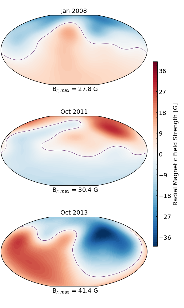

The awsom simulations can be prone to oscillation, but usually the solution will converge quite well with very minimal oscillation in global wind parameters such as mass-loss rate, open magnetic flux, and angular-momentum loss rate. For our purposes, we assume a simulation to be converged when these three variables oscillate below 5%. Our mass-loss rate benchmarked January 2008 simulation is quite close to the observed values given by Wood & Linsky 1998. We see this increase for the final epoch simulated, with a increase in the mass-loss rate between Jan 2008 and Oct 2013. Our simulations result in mass loss rates that are times the solar mass loss rate. Angular momentum loss rates range from erg in October 2011 to erg in October 2013. Finley et al. 2019 used semi-analytical relations to estimate the mass-loss and angular momentum loss variability of this star. The values we find agree very well with their calculations, including the variability trend for each epoch. This is shown in Figure 2. We see excellent alignment in the 2008 epoch. In Figure 9 we show the velocity and magnetic field structure of the stellar wind solutions for each epoch.
III Modelling coronal mass ejections from Eri
Our CME simulations are initialised using a TD flux rope model (Titov & Démoulin 1999) which is implemented within the SWMF framework using the two temperature model described by Meng et al. 2015. This places a twisted force-free flux rope at the inner boundary of our simulations, with footpoints anchored in the stellar surface. It creates a strong, localised, magnetic bipole on the surface of the star. The sudden disequilibrium between magnetic and pressure forces causes the flux rope to erupt outwards into the corona and stellar wind. The model has eight free parameters, which control the size, shape, orientation, mass and free magnetic energy of the flux tube. These free parameters for each CME simulation carried out in this work are as follows: Longitude (), Latitude (, , or ), Orientation/tilt (), major radius (Rmaj; 128 Mm), minor radius (Rmin; 20 Mm), depth (; 1 Mm), current (ICME; A), mass (MCME; g). This configuration gives a loop length Mm. For an in depth discussion on these parameters, we direct the reader to Titov & Démoulin 1999 and Meng et al. 2015. These parameters result in a CME flux rope such as that visualised in Figure 3. Since we do not have rigid constraints on eruption location for CMEs on a star like Eri, we simulate three CMEs for each stellar wind solution. One CME is positioned near the equator (latitude of ), and the other two are polar (latitude of and ). Note that the observed stellar magnetic field is less constrained in the southern hemisphere of the star due to the stellar inclination with respect to Earth. Therefore we conduct CME eruption simulations in both hemispheres to compare and contrast the effect this has on CME shock formation and propagation.
The size and current set the amount of free magnetic energy (ECME) in the flux tube. We choose these parameters so that E erg. This magnetic energy is 3 orders of magnitude greater than those estimated for solar CMEs (Vourlidas et al. 2000), and yet still small (1000 times less) compared to estimates for some M dwarf eruptive events (Alvarado-Gómez et al. 2018). The initial mass of the CME is constrained by taking the X-ray flux of flares on Eri (Coffaro et al. 2020), and comparing that to the X-ray flux - CME-mass relationship for the Sun (Aarnio et al. 2011). This results in a mass of , large for a solar CME, but is still considered small ( times less) compared to some estimations for CMEs on other stars (Moschou et al. 2019). Due to the elevated X-ray fluxes, stronger magnetic fields of Eri (Petit et al. 2021), and its young nature, the energy related to our CME constructed here is well within extended observational trends for a star of this kind.

| Sim | ur [km s-1] | MCME [g] | Ek [erg] |
|---|---|---|---|
| 2008 Eq | 2602 | ||
| 2008 NP | 2730 | ||
| 2008 SP | 2229 | ||
| 2011 Eq | 2685 | ||
| 2011 NP | 2993 | ||
| 2011 SP | 2247 | ||
| 2013 Eq | 1527 | ||
| 2013 NP | 2110 | ||
| 2013 SP | 2476 |
Figure 4 shows an example of a simulated CME, 10 minutes post-eruption. To define the isocontour surrounding the CME volume, we compare plasma density at the current timestep to the plasma density for the steady-state stellar wind solution. A ratio of between these values defines the isocontour (similar to the definition in Alvarado-Gómez et al. 2019). In reality, the CME shock and radio emission will precede the high density region of a CME by some finite distance. The shock location can alternatively be delineated by finding the maximum entropy gradient in the plasma (Schmidt et al. 2013), discussed in Appendix C. From our simulations we calculate the distance between the CME body and entropy gradient shock location to be 0.2 R⋆. This means that the plasma frequencies calculated in this work are upper limits, with the actual value marginally lower (by a factor of 1–2) due to the shock location having a slightly lower plasma density.
To determine if the CME produces a shock, it is important to consider the Alfvén Mach number,
| (1) |
where is the stellar wind velocity, is the CME velocity, and the Alfvén velocity is . This CME Mach number is depicted in Figure 4 as a scatter of spheres across the surface of the CME, where the colour and size are proportional to the Alfvénic Mach number. From solar studies, it appears that type II radio bursts are most likely to originate from regions of high Alfvénic Mach number, or low Alfvén velocity, and quasi-perpendicular geometries (Zucca et al. 2014; Zucca et al. 2018; Maguire et al. 2020).

The 2013 equatorial epoch presented the slowest CME velocities from our simulated sample (see Table 4 and Figure 8 in Appendix A). This is expected as the strongest azimuthal magnetic fields are present in this case. This strong azimuthal field partially impedes the CME, providing stronger magnetic pressure resisting expansion. For this reason, at the 10 minute mark, Figure 5 shows the equatorial CMEs as closest to the stellar surface, particularly so in the case of October 2013, which has the strongest surface magnetic field of all epochs. Table 4 shows the CME velocity, total mass at 1 hour, and kinetic energy of each CME shown in Figure 5. The CME mass here is defined as the mass within the isocontours defined above, with velocities greater than the escape velocity () of the star. Note that only one CME has a mass greater than the initial flux rope mass, which is the 2011 northern polar CME. This can occur as the CME sweeps up extra material and carries it outwards. The other cases show a reduced mass from the initial flux rope mass, which can be explained by material being trapped close to the stellar surface, or slowing below the requires escape velocity. If these CMEs occurred at a rate near the upper end of the relation described by Odert et al. 2017 (Figure 2 within; assuming between 1.5 and 1.8), we could expect these CMEs to carry away M⊙ yr-1 (). The lower range of this estimate amounts to of the stellar wind mass-loss rate for our January 2008 wind simulation, or as high as . This is a significant proportion of the stellar mass carried away in eruptive events. At the lower end of the scale of the CME frequency relation from Odert et al. 2017, we would still expect of the stellar mass-loss to occur due to CMEs. Note that we assume a uniform CME-mass relation from our simulations here, not the CME-mass distribution in Odert et al. 2017.
Comparing the northern and southern hemisphere CMEs shows no clear trend between the two cases. We see a difference in eruption velocity (Table 4) for each scenario. While in 2008 and 2011 the northern CMEs display an average velocity of 624 km s-1 faster than their southern counterparts, the 2013 shows the reverse scenario, with the northern CME being 366 km s-1 slower than the southern CME. This lack of a trend is evident in CME kinetic energy where the northern event has the largest value in the 2011, but the reverse is true in the 2008 and 2013 epochs. Given that only the northern hemisphere of the stellar surface magnetic field was constrained through ZDI, it is surprising that we do not see more pronounced differences in the opposing CME events.
IV CME Radio Emission and variability
While M dwarfs have been the focus of possible type II radio bursts sources for some time (Villadsen 2017; Crosley & Osten 2018a; Crosley & Osten 2018b), recent numerical studies have suggested that the coronal and wind environment around these vibrant magnetic stars is not conducive to strong type II bursts (Alvarado-Gómez et al. 2018; Alvarado-Gómez et al. 2019). In some cases a strong azimuthal magnetic field can cause complete suppression of an erupting CME resulting in a failed eruption, and in others there are partial eruptions (or impeded in some way, similar to our October 2013 CME simulation above). Additionally, the fast stellar winds of these stars (e.g. Kavanagh et al. 2021) means the CMEs only become super-Alfvénic at large distances, meaning the density is greatly reduced, along with the plasma frequency, compared to the lower stellar atmosphere making detection more difficult (Alvarado-Gómez et al. 2020). Solar-type stars such as Eri present an attractive alternative to the much more magnetic M dwarfs. As a younger and more active star, it displays frequent flaring (Audard et al. 2000; Coffaro et al. 2020) combined with a background magnetic field whose strength is insufficient to confine any putative CME eruption, which we see in our results in Figure 5.
Since the type II emission mechanism is coherent plasma emission due to Langmuir wave growth (see Melrose 2017 for an in depth discussion on astrophysical plasma emission mechanisms), we expect any emitted radio wave to occur near the plasma frequency ( Hz), in this work we assume the emission occurs at the plasma frequency. In reality, the emission would need to occur above the local plasma frequency in order to propagate without absorption. Schmidt et al. 2013 use the BAT-R-US code to simulate a solar eruptive CME event, which they combine with their stochastic growth theory for type II radio burst emission and successfully replicate the type II burst observed with the WIND spacecraft on 2011 February 15 UTC. In our simulations, we extract the plasma frequency information from the volume of the CME front at each timestep and use this to create pseudo-spectra, which consist of the frequency of the emission, but not the intensity.
Eri has been observed many times at various radio frequencies (Bastian et al. 2018; Rodríguez et al. 2019; Suresh et al. 2020). Each of these works has achieved detections of Eri at frequencies above 1 GHz. Figure 4 in Suresh et al. 2020 collates these observations into a radio spectrum of the star above 2 GHz, including millimetre observations (MacGregor et al. 2015; Booth et al. 2017; Lestrade & Thilliez 2015; Chavez-Dagostino et al. 2016). While these observations are interesting for other reasons, such as the stellar wind constraint provided by Suresh et al. 2020, the transient type II radio bursts occur at much lower frequencies (420 MHz maximum, 110 MHz average, Umuhire et al. 2021). George & Stevens 2007 observed Eri at 157 MHz using the GMRT, but did not detect anything. They were able to place upper limits of 7.8 mJy on the radio emission from the system. These observations were aiming to detect exoplanetary radio emission, only amounted to 4 hours on source, and were significantly affected by radio-frequency interference. To date there have been no detections of Eri at this low frequency range.


Pseudo-spectra are shown in Figure 6 and depict the range of possible emission frequencies from each CME at each timestep in our simulations. The boxes show the median plasma frequency of the CME (horizontal black lines), extracted from the isosurfaces of the CMEs shown in Figure 5, and the inter-quartile range for the CME volume (25% – 75% of the distribution). The white nabla symbols mark the 2nd harmonic, which is seen to have strong emission for solar CMEs. Typically, outliers are denoted as fliers in boxplots, however we have removed them as they render Figure 6 unreadable. Outliers in this case are due to both high and low density artefacts in the CME isosurface definition and pockets of high density material appearing near the stellar surface. This results in many thousands of fliers due to the high resolution of our simulation grid. Note that due to the shock definition, it is difficult to determine exact emission frequencies without rigorous follow-up observations. For this reason, frequencies in Figure 6 provide an upper-limit and could be overestimated by a factor of 2 (see Appendix C). Depending on the magnetic field epoch, and the location of eruption, the window of opportunity for a positive detection of these events is usually 10 minutes for fundamental emission using LOFAR (LOw Frequency ARray). However, variation in the October 2011 magnetic field (Figure 6, top right panel) shows extended fundamental emission up to 30 minutes above the frequency range of LOFAR. Harmonic emission retains a frequency above 10 MHz for an additional 10 minutes for most cases. These times are much shorter for the other telescope frequency ranges, with fundamental emission only remaining above this level for 1-5 minutes for the MWA (Murchison Widefield Array) and LWA (Long Wavelength Array). Note that the emission is expected to exceed 150 MHz for only a short time (1 min) and in some cases it is only the harmonic emission that does this. This, combined with sensitivity issues of the instrument at these short timescales and RFI, could explain the non-detection of any emission by George & Stevens 2007. It is important to note that these pseudo-spectra do not give any information on the emission intensity, and so we can not say if emission would be strong enough to actually be detected by each of these instruments. This emission could change given more precise particle acceleration and radiative transfer descriptions. While we do not carry out this analysis in this work, the simulations presented here could be used to apply a more rigorous analysis on the radiation generated by electron beams at the CME shock location (e.g. using quasi-linear theory, Reid & Kontar 2015; or stochastic growth theory, Knock et al. 2001; Schmidt & Cairns 2012a; Schmidt & Cairns 2012b).
On the Sun, the acceleration sites in type II related CMEs seem to vary. Zucca et al. 2018 estimated one type II event on the Sun originated from plasma on the CME flank with Mach numbers in the range of 1.4–1.6. Maguire et al. 2020 found a solar type II radio burst generated from the CME nose with similar Mach numbers, which ceases as the CME progresses, despite increasing Mach number. The exact location of bursts in the radio is further complicated by strong refraction in the solar corona. This makes it difficult to accurately locate solar radio bursts (see Kontar et al. 2019 for a discussion on solar coronal scattering, and Chrysaphi et al. 2018; Chen et al. 2020 for detailed type II and III radio burst scattering analysis respectively). Morosan et al. 2021 pointed out that slower solar CMEs ( 200 km s-1) are more likely to be associated with type II bursts, while faster CMEs are likely associated with type IV bursts. From Figure 5, the range of Alfvénic Mach numbers in the plasma are shown as scattered spheres. They reach much higher values than the ones cited previously for solar CME events. However, it is clear from the October 2011 simulations that the largest Mach numbers can appear at any location around the CME surface. For the equatorial case we see high Alfvén Mach numbers in the CME flanks, however for the polar cases the highest Alfvén Mach numbers appear on the nose. The location of the strongest beamed electrons that would drive a type II event on these CMEs is also dependent on the orientation of the shock front and plasma velocity components to the ambient magnetic field (Yuan et al. 2008; Schmidt & Cairns 2012b). See Appendix A for examples of velocity component distributions of our CME events.
The simulated October 2011 equatorial CME presents the highest Alfvén Mach numbers of any of our CMEs (also evident in Figure 6). In the case of this eruption, the volume it erupted into was particularly low density in the steady wind solution. This gives rise to a large defined CME structure which can produce very high Alfvén velocities due to the low density in the wind previously.
Keeping the caveats of the pseudo-spectra in mind, i.e. uncertainty in radio burst location along the CME front and radio intensity, it remains likely that the maximum time these events on Eri would remain within the spectral coverage is 20-30 minutes post-eruption for the polar CMEs, with a slight chance of harmonic detection for up to 50 minutes. If we compare the differences between the equatorial and polar spectra, we find that equatorial CMEs tend to exhibit much higher emission frequencies for a longer period of time post-eruption. This is likely due to their slower nature, being confined by more restrictive closed-magnetic field lines. This means they are embedded in a higher density plasma for a longer time. It is clear that the magnetic geometry and strength has a strong affect on the detectability of these events. In the synthetic spectra for the polar cases, we see a much smaller range and a faster decline of the median plasma frequency within the CME. This suggests that polar CMEs on Eri could have a shorter detectable window than their lower latitude counterparts. These effects are evident in Figure 5, where we see the left column of equatorial CMEs exhibit much stronger flank formations, whereas the polar CMEs retain a more globular shape. The exception is the October 2011 northern polar CME which retains a dense globular formation near the stellar surface which might skew the pseudo-spectrum towards higher plasma frequencies. It is important to remember that these pseudo-spectra are just a guide for expected emission frequencies, and actual emission frequency could differ depending on the location of strongest shock formation.
The October 2013 equatorial CME experiences a serious fragmentation after 10 minutes, and is the slowest of the CMEs. For this reason it could be considered to be partially suppressed by the stellar magnetic field. As this epoch has the strongest magnetic field of those considered in this work, it makes sense that it is the only one for which we see partial suppression.
Of course, much more massive events, with larger flux rope masses, would likely give rise to higher plasma frequencies surrounding the shock, making them detectable for a longer period of time. However, in our simulations, our flux rope mass of g is at the larger end for solar CMEs. Given that Eri is a solar-type star, we proposed this flux rope mass was a good approximation of expected values. Moschou et al. 2019 estimated that some active stars could exhibit CMEs with masses 5-6 orders of magnitude larger than the value we used in this work. These super-CMEs are more likely to exist on the most active of M dwarfs due to their strong stellar magnetic fields and intense flaring activity.
V Conclusions
We simulated nine different CMEs for Eridani across three different epochs. From our assumed CME setup, each case erupted violently into the surrounding stellar wind and produced a shock. These shocks were estimated to produce type II burst radio emission as high as 165 MHz at the fundamental frequencies, and twice this value for their 2nd harmonics. The duration that these events would remain observable was 10-20 minutes in most cases assuming an ionospheric cutoff of 10 MHz. In some particular cases, this time-frame was slightly extended to minutes (October 2011 - Polar North CME).
We found little clear evidence of the magnetic cycle of Eridani affecting the CMEs across the epochs January 2008 to October 2013. Each epoch produced strong shocked material that was ejected from the stellar surface in each eruptive location. The lack of magnetic confinement and large Alfvén Mach numbers are promising signs of type II radio emission from these events. In the case of the 2013 epoch, we see the equatorial CME is significantly slower than other equatorial eruptions at different epochs. This is the only evidence of magnetic variability affecting the CMEs, which results in lower Alfvén Mach numbers, but a longer duration embedded in high density plasma. Eruption location on the stellar surface has an effect on the CME propagation, closely tied to magnetic geometry. We found CMEs that erupt through regions of closed magnetic field are slightly impeded and exhibit slower speeds and lower Alfvén Mach numbers, indicative of weaker shocks. This could result in much weaker type II bursts, or perhaps no formation of type II emission at all. However, if type II emission occurs, it would result in longer observable windows from low-frequency telescopes.
In the future, these CME simulations on a nearby K dwarf star could be used as inputs to more rigorous particle and radiative simulations of electron beams produced by these shocks. Particle-in-cell simulations would give precise electron distributions and radiative models such as quasi-linear simulations or stochastic growth theory could calculate emitted flux density from the electron beams. This type of work could place tight constraints on the flux densities expected from typical CME events on Eridani, and whether they should be detectable from the ground with current (i.e. LOFAR, LWA, MWA) or future (e.g. SKA-Low) radio telescopes.
Simulation data is made available through zenodo (Ó Fionnagáin et al. 2021).
TBL(NARVAL). Data are made available through the PolarBase archive (Petit et al. 2014; http://polarbase.irap.omp.eu/).
ICHEC Kay HPC.
Appendix A Velocity Distributions
We show the magnitude of the orthogonal components of the velocity to the magnetic field within the CME shocks in our simulations in Figure 7. In particular we show the distribution of each equatorial CME at the 10-minute timestep in our simulations. These components can be derived from our awsom simulations by carrying out a vector projection of the velocity onto the magnetic vector where
| (A1) |
| (A2) |
We can see that the 2011 epoch has the longest tailed distribution in both and . These electron distributions could be used as background distributions for electron beams and radiative emission simulations in future work. Figure 8 shows the maximum velocity of the CME shock over the simulation time for each case. We see that the October 2013 equatorial case has a significantly lower velocity throughout.

Appendix B Stellar wind simulations
Section II describes the AWSOM wind models that we use as a starting point for our CME simulations. The solutions to these stellar winds are shown here, pre-eruptive event in Figure 9. Global wind variables for these solutions are plotted in Figure 2.

We compare the thermal radio spectrum calculated from our 3D MHD wind simulations to the radio observations from MacGregor et al. 2015; Booth et al. 2017; Lestrade & Thilliez 2015; Bastian et al. 2018; Rodríguez et al. 2019; Suresh et al. 2020 in Figure 10. We find a much lower flux density for the wind spectra for each epoch simulated here, compared to the 6-20 GHz range of observations (referenced previously and collated in Suresh et al. 2020). This supports conclusions drawn by Bastian et al. 2018, that these radio detections were indeed due to high density active regions. Alternatively these could be chromospheric detections, which is also much denser than the stellar wind, giving a higher flux density. Our simulations are in agreement with these data points in that our wind is optically thin in the same regime. This difference in estimated spectra is not unexpected given the large difference in mass-loss rate from the different wind estimates (i.e. Wood 2018 vs. Suresh et al. 2020).
Appendix C Shock Definition
In this work, we use the edge of the CME to define the shock location and the plasma frequency of the emission. In reality, the shock would exist preceding the CME itself. Schmidt et al. 2013 used the entropy gradient in their simulation to define the shock location and normal. Using this method in our simulation results in the shock front shown in Figure 11. However, we avoided using this method as it resulted in a large number of artefacts incorrectly attributed to the shock, skewing our estimates of the plasma frequency for the shock. We can see that the defined shock contours (blue-pink) using the entropy gradient method surround the delineated CME isosurface. This definition extends further radially than the CME isosurface, resulting is some lower densities at this point. As a result, our calculated plasma frequencies are upper limits at each timestep in our simulations, and the true value is likely between lower in frequency. More robust shock delineation and radio emission simulations are necessary to more accurately describe the type II bursts.

References
- Aarnio et al. (2012) Aarnio, A. N., Matt, S. P., & Stassun, K. G. 2012, ApJ, 760, 9, doi: 10.1088/0004-637X/760/1/9
- Aarnio et al. (2011) Aarnio, A. N., Stassun, K. G., Hughes, W. J., & McGregor, S. L. 2011, Sol. Phys., 268, 195, doi: 10.1007/s11207-010-9672-7
- Airapetian et al. (2016) Airapetian, V. S., Glocer, A., Gronoff, G., Hébrard, E., & Danchi, W. 2016, Nature Geoscience, 9, 452, doi: 10.1038/ngeo2719
- Alvarado-Gómez et al. (2018) Alvarado-Gómez, J. D., Drake, J. J., Cohen, O., Moschou, S. P., & Garraffo, C. 2018, ApJ, 862, 93, doi: 10.3847/1538-4357/aacb7f
- Alvarado-Gómez et al. (2019) Alvarado-Gómez, J. D., Garraffo, C., Drake, J. J., et al. 2019, ApJ, 875, L12, doi: 10.3847/2041-8213/ab1489
- Alvarado-Gómez et al. (2020) Alvarado-Gómez, J. D., Drake, J. J., Fraschetti, F., et al. 2020, ApJ, 895, 47, doi: 10.3847/1538-4357/ab88a3
- Argiroffi et al. (2019) Argiroffi, C., Reale, F., Drake, J., et al. 2019, Nature Astronomy, 3, 742
- Audard et al. (2000) Audard, M., Güdel, M., Drake, J. J., & Kashyap, V. L. 2000, ApJ, 541, 396, doi: 10.1086/309426
- Baines & Armstrong (2012) Baines, E. K., & Armstrong, J. T. 2012, ApJ, 744, 138, doi: 10.1088/0004-637X/744/2/138
- Barnes (2007) Barnes, S. A. 2007, ApJ, 669, 1167, doi: 10.1086/519295
- Bastian et al. (2018) Bastian, T. S., Villadsen, J., Maps, A., Hallinan, G., & Beasley, A. J. 2018, ApJ, 857, 133, doi: 10.3847/1538-4357/aab3cb
- Booth et al. (2017) Booth, M., Dent, W. R. F., Jordán, A., et al. 2017, MNRAS, 469, 3200, doi: 10.1093/mnras/stx1072
- Boro Saikia et al. (2020) Boro Saikia, S., Jin, M., Johnstone, C. P., et al. 2020, A&A, 635, A178, doi: 10.1051/0004-6361/201937107
- Burton & MacGregor (2021) Burton, K., & MacGregor, M. A. 2021, in American Astronomical Society Meeting Abstracts, Vol. 53, American Astronomical Society Meeting Abstracts, 124.07
- Carley et al. (2020) Carley, E. P., Vilmer, N., & Vourlidas, A. 2020, Frontiers in Astronomy and Space Sciences, 7, 79, doi: 10.3389/fspas.2020.551558
- Chandran et al. (2011) Chandran, B. D. G., Dennis, T. J., Quataert, E., & Bale, S. D. 2011, ApJ, 743, 197, doi: 10.1088/0004-637X/743/2/197
- Chavez-Dagostino et al. (2016) Chavez-Dagostino, M., Bertone, E., Cruz-Saenz de Miera, F., et al. 2016, MNRAS, 462, 2285, doi: 10.1093/mnras/stw1363
- Chen et al. (2020) Chen, X., Kontar, E. P., Chrysaphi, N., et al. 2020, ApJ, 905, 43, doi: 10.3847/1538-4357/abc24e
- Chrysaphi et al. (2018) Chrysaphi, N., Kontar, E. P., Holman, G. D., & Temmer, M. 2018, ApJ, 868, 79, doi: 10.3847/1538-4357/aae9e5
- Coffaro et al. (2020) Coffaro, M., Stelzer, B., Orlando, S., et al. 2020, A&A, 636, A49, doi: 10.1051/0004-6361/201936479
- Cranmer (2017) Cranmer, S. R. 2017, ApJ, 840, 114, doi: 10.3847/1538-4357/aa6f0e
- Crosley & Osten (2018a) Crosley, M. K., & Osten, R. A. 2018a, ApJ, 856, 39, doi: 10.3847/1538-4357/aaaec2
- Crosley & Osten (2018b) —. 2018b, ApJ, 862, 113, doi: 10.3847/1538-4357/aacf02
- Donati & Landstreet (2009) Donati, J. F., & Landstreet, J. D. 2009, ARA&A, 47, 333, doi: 10.1146/annurev-astro-082708-101833
- Drake et al. (2019) Drake, J., Alvarado-Gómez, J. D., Airapetian, V., et al. 2019, BAAS, 51, 113. https://arxiv.org/abs/1903.12338
- Drake et al. (2013) Drake, J. J., Cohen, O., Yashiro, S., & Gopalswamy, N. 2013, ApJ, 764, 170, doi: 10.1088/0004-637X/764/2/170
- Finley et al. (2019) Finley, A. J., See, V., & Matt, S. P. 2019, ApJ, 876, 44, doi: 10.3847/1538-4357/ab12d2
- Gaia Collaboration et al. (2021) Gaia Collaboration, Brown, A. G. A., Vallenari, A., et al. 2021, A&A, 649, A1, doi: 10.1051/0004-6361/202039657
- Garraffo et al. (2017) Garraffo, C., Drake, J. J., Cohen, O., Alvarado-Gómez, J. D., & Moschou, S. P. 2017, ApJ, 843, L33, doi: 10.3847/2041-8213/aa79ed
- George & Stevens (2007) George, S. J., & Stevens, I. R. 2007, MNRAS, 382, 455, doi: 10.1111/j.1365-2966.2007.12387.x
- Gombosi et al. (2018) Gombosi, T. I., van der Holst, B., Manchester, W. B., & Sokolov, I. V. 2018, Living Rev. Sol. Phys., 15, 4, doi: 10.1007/s41116-018-0014-4
- Gopalswamy et al. (2008) Gopalswamy, N., Yashiro, S., Xie, H., et al. 2008, ApJ, 674, 560, doi: 10.1086/524765
- Gray & Baliunas (1995) Gray, D. F., & Baliunas, S. L. 1995, ApJ, 441, 436, doi: 10.1086/175368
- Greaves et al. (1998) Greaves, J. S., Holland, W. S., Moriarty-Schieven, G., et al. 1998, ApJ, 506, L133, doi: 10.1086/311652
- Harris et al. (2020) Harris, C. R., Millman, K. J., van der Walt, S. J., et al. 2020, Nature, 585, 357–362, doi: 10.1038/s41586-020-2649-2
- Hatzes et al. (2000) Hatzes, A. P., Cochran, W. D., McArthur, B., et al. 2000, ApJ, 544, L145, doi: 10.1086/317319
- Hazra et al. (2021) Hazra, G., Vidotto, A., et al. 2021, subm.
- Heiter et al. (2015) Heiter, U., Jofré, P., Gustafsson, B., et al. 2015, A&A, 582, A49, doi: 10.1051/0004-6361/201526319
- Hollweg (1976) Hollweg, J. V. 1976, 81, 1649
- Hunter (2007) Hunter, J. D. 2007, Computing in Science & Engineering, 9, 90, doi: 10.1109/MCSE.2007.55
- Janson et al. (2008) Janson, M., Reffert, S., Brandner, W., et al. 2008, A&A, 488, 771, doi: 10.1051/0004-6361:200809984
- Jeffers et al. (2014) Jeffers, S. V., Petit, P., Marsden, S. C., et al. 2014, A&A, 569, A79, doi: 10.1051/0004-6361/201423725
- Jin et al. (2012) Jin, M., Manchester, W. B., van der Holst, B., et al. 2012, ApJ, 745, 6, doi: 10.1088/0004-637X/745/1/6
- Kavanagh et al. (2021) Kavanagh, R. D., Vidotto, A. A., Klein, B., et al. 2021, MNRAS, 504, 1511, doi: 10.1093/mnras/stab929
- Kharayat et al. (2021) Kharayat, H., Joshi, B., & Chandra, R. 2021, Ap&SS, 366, 24, doi: 10.1007/s10509-021-03930-w
- Knock et al. (2001) Knock, S. A., Cairns, I. H., Robinson, P. A., & Kuncic, Z. 2001, J. Geophys. Res., 106, 25041, doi: 10.1029/2001JA000053
- Kontar et al. (2019) Kontar, E. P., Chen, X., Chrysaphi, N., et al. 2019, ApJ, 884, 122, doi: 10.3847/1538-4357/ab40bb
- Kumari et al. (2017) Kumari, A., Ramesh, R., Kathiravan, C., & Gopalswamy, N. 2017, ApJ, 843, 10, doi: 10.3847/1538-4357/aa72e7
- Lehmann et al. (2015) Lehmann, L. T., Künstler, A., Carroll, T. A., & Strassmeier, K. G. 2015, Astronomische Nachrichten, 336, 258, doi: 10.1002/asna.201412162
- Leitzinger et al. (2011) Leitzinger, M., Odert, P., Ribas, I., et al. 2011, A&A, 536, A62, doi: 10.1051/0004-6361/201015985
- Leitzinger et al. (2020) Leitzinger, M., Odert, P., Greimel, R., et al. 2020, MNRAS, 493, 4570, doi: 10.1093/mnras/staa504
- Lestrade & Thilliez (2015) Lestrade, J.-F., & Thilliez, E. 2015, A&A, 576, A72, doi: 10.1051/0004-6361/201425422
- Lionello et al. (2009) Lionello, R., Linker, J. A., & Mikić, Z. 2009, ApJ, 690, 902, doi: 10.1088/0004-637X/690/1/902
- MacGregor et al. (2015) MacGregor, M. A., Wilner, D. J., Andrews, S. M., Lestrade, J.-F., & Maddison, S. 2015, ApJ, 809, 47, doi: 10.1088/0004-637X/809/1/47
- Maguire et al. (2020) Maguire, C. A., Carley, E. P., McCauley, J., & Gallagher, P. T. 2020, A&A, 633, A56, doi: 10.1051/0004-6361/201936449
- Mamajek & Hillenbrand (2008) Mamajek, E. E., & Hillenbrand, L. A. 2008, ApJ, 687, 1264, doi: 10.1086/591785
- Mawet et al. (2019) Mawet, D., Hirsch, L., Lee, E. J., et al. 2019, AJ, 157, 33, doi: 10.3847/1538-3881/aaef8a
- Melrose (2017) Melrose, D. B. 2017, Reviews of Modern Plasma Physics, 1, 5, doi: 10.1007/s41614-017-0007-0
- Meng et al. (2015) Meng, X., Van der Holst, B., Tóth, G., & Gombosi, T. I. 2015, MNRAS, 454, 3697, doi: 10.1093/mnras/stv2249
- Metcalfe et al. (2013) Metcalfe, T. S., Buccino, A. P., Brown, B. P., et al. 2013, ApJ, 763, L26, doi: 10.1088/2041-8205/763/2/L26
- Morosan et al. (2021) Morosan, D. E., Kumari, A., Kilpua, E. K. J., & Hamini, A. 2021, A&A, 647, L12, doi: 10.1051/0004-6361/202140392
- Moschou et al. (2019) Moschou, S.-P., Drake, J. J., Cohen, O., et al. 2019, ApJ, 877, 105, doi: 10.3847/1538-4357/ab1b37
- Ó Fionnagáin et al. (2021) Ó Fionnagáin, D., Vidotto, A. A., Petit, P., et al. 2021, MNRAS, 500, 3438, doi: 10.1093/mnras/staa3468
- Ó Fionnagáin et al. (2021) Ó Fionnagáin, D., et al. 2021, Simulations of Coronal Mass Ejections on the star e Eridani, v 0.1, Zenodo, doi: 10.5281/zenodo.5575241
- Odert et al. (2017) Odert, P., Leitzinger, M., Hanslmeier, A., & Lammer, H. 2017, MNRAS, 472, 876, doi: 10.1093/mnras/stx1969
- Osten et al. (2013) Osten, R., Livio, M., Lubow, S., et al. 2013, ApJ, 765, L44, doi: 10.1088/2041-8205/765/2/L44
- Osten & Wolk (2015) Osten, R. A., & Wolk, S. J. 2015, ApJ, 809, 79, doi: 10.1088/0004-637X/809/1/79
- pandas development team (2020) pandas development team, T. 2020, pandas-dev/pandas: Pandas, latest, Zenodo, doi: 10.5281/zenodo.3509134
- Petit et al. (2014) Petit, P., Louge, T., Théado, S., et al. 2014, PASP, 126, 469, doi: 10.1086/676976
- Petit et al. (2021) Petit, P., Folsom, C. P., Donati, J. F., et al. 2021, A&A, 648, A55, doi: 10.1051/0004-6361/202040027
- Powell et al. (1999) Powell, K. G., Roe, P. L., Linde, T. J., Gombosi, T. I., & De Zeeuw, D. L. 1999, Journal of Computational Physics, 154, 284, doi: 10.1006/jcph.1999.6299
- Reid & Kontar (2015) Reid, H. A. S., & Kontar, E. P. 2015, A&A, 577, A124, doi: 10.1051/0004-6361/201425309
- Riley et al. (2019) Riley, A. H., Strigari, L. E., Porter, T. A., et al. 2019, The Astrophysical Journal, 878, 8
- Rodríguez et al. (2019) Rodríguez, L. F., Lizano, S., Loinard, L., et al. 2019, The Astrophysical Journal, 871, 172, doi: 10.3847/1538-4357/aaf9a6
- Schmidt & Cairns (2012a) Schmidt, J. M., & Cairns, I. H. 2012a, Journal of Geophysical Research (Space Physics), 117, A04106, doi: 10.1029/2011JA017318
- Schmidt & Cairns (2012b) —. 2012b, Journal of Geophysical Research (Space Physics), 117, A11104, doi: 10.1029/2012JA017932
- Schmidt et al. (2013) Schmidt, J. M., Cairns, I. H., & Hillan, D. S. 2013, ApJ, 773, L30, doi: 10.1088/2041-8205/773/2/L30
- Segura et al. (2010) Segura, A., Walkowicz, L. M., Meadows, V., Kasting, J., & Hawley, S. 2010, Astrobiology, 10, 751, doi: 10.1089/ast.2009.0376
- Sindhuja & Gopalswamy (2020) Sindhuja, G., & Gopalswamy, N. 2020, The Astrophysical Journal, 889, 104
- Sokolov et al. (2013) Sokolov, I. V., van der Holst, B., Oran, R., et al. 2013, ApJ, 764, 23, doi: 10.1088/0004-637X/764/1/23
- Spitzer & Härm (1953) Spitzer, L., & Härm, R. 1953, Physical Review, 89, 977, doi: 10.1103/PhysRev.89.977
- Suresh et al. (2020) Suresh, A., Chatterjee, S., Cordes, J. M., Bastian, T. S., & Hallinan, G. 2020, ApJ, 904, 138, doi: 10.3847/1538-4357/abc004
- Titov & Démoulin (1999) Titov, V. S., & Démoulin, P. 1999, A&A, 351, 707
- Umuhire et al. (2021) Umuhire, A. C., Gopalswamy, N., Uwamahoro, J., et al. 2021, Sol. Phys., 296, 27, doi: 10.1007/s11207-020-01743-8
- Valenti & Fischer (2005) Valenti, J. A., & Fischer, D. A. 2005, ApJS, 159, 141, doi: 10.1086/430500
- van der Holst et al. (2010) van der Holst, B., Manchester, W. B., I., Frazin, R. A., et al. 2010, ApJ, 725, 1373, doi: 10.1088/0004-637X/725/1/1373
- Van Der Holst et al. (2014) Van Der Holst, B., Sokolov, I. V., Meng, X., et al. 2014, ApJ, 782, 81, doi: 10.1088/0004-637X/782/2/81
- Vida et al. (2019) Vida, K., Leitzinger, M., Kriskovics, L., et al. 2019, A&A, 623, A49, doi: 10.1051/0004-6361/201834264
- Vida et al. (2016) Vida, K., Kriskovics, L., Oláh, K., et al. 2016, A&A, 590, A11, doi: 10.1051/0004-6361/201527925
- Villadsen (2017) Villadsen, J. R. 2017, PhD thesis, California Institute of Technology
- Vourlidas et al. (2000) Vourlidas, A., Subramanian, P., Dere, K. P., & Howard, R. A. 2000, ApJ, 534, 456, doi: 10.1086/308747
- Waskom (2021) Waskom, M. L. 2021, Journal of Open Source Software, 6, 3021, doi: 10.21105/joss.03021
- Wood (2018) Wood, B. E. 2018, in Journal of Physics Conference Series, Vol. 1100, Journal of Physics Conference Series, 012028, doi: 10.1088/1742-6596/1100/1/012028
- Wood & Linsky (1998) Wood, B. E., & Linsky, J. L. 1998, ApJ, 492, 788, doi: 10.1086/305077
- Yashiro & Gopalswamy (2009) Yashiro, S., & Gopalswamy, N. 2009, in Universal Heliophysical Processes, ed. N. Gopalswamy & D. F. Webb, Vol. 257, 233–243, doi: 10.1017/S1743921309029342
- Yuan et al. (2008) Yuan, X., Cairns, I. H., & Robinson, P. A. 2008, Journal of Geophysical Research (Space Physics), 113, A08109, doi: 10.1029/2008JA013268
- Zucca et al. (2014) Zucca, P., Carley, E. P., Bloomfield, D. S., & Gallagher, P. T. 2014, A&A, 564, A47, doi: 10.1051/0004-6361/201322650
- Zucca et al. (2018) Zucca, P., Morosan, D. E., Rouillard, A. P., et al. 2018, A&A, 615, A89, doi: 10.1051/0004-6361/201732308