跳到论文正文
W Papers独立论文阅读器 arXiv:2111.02227 论文正文 计算阅读时间 · 0%
引用这篇论文根据当前论文元数据生成,正式投稿前建议核对。


License: CC BY 4.0
arXiv:2111.02227v3 [math.FA] 06 Apr 2022

On foundational discretization barriers in STFT phase retrieval

Philipp Grohs*,†,‡ Address: *Faculty of Mathematics, University of Vienna, Oskar-Morgenstern-Platz 1, 1090 Vienna, Austria Address: †Research Network DataScience@UniVie, University of Vienna, Kolingasse 14-16, 1090 Vienna, Austria Address: ‡Johann Radon Institute of Applied and Computational Mathematics, Austrian Academy of Sciences, Altenbergstrasse 69, 4040 Linz, Austria Email address: philipp.grohs@univie.ac.at, philipp.grohs@oeaw.ac.at and Lukas Liehr* Email address: lukas.liehr@univie.ac.at
Date: August 11, 2026
Abstract.

We prove that there exists no window function g∈L2​(ℝ)g\in{L^{2}({\mathbb{R}})} and no lattice ℒ⊂ℝ2\mathcal{L}\subset{\mathbb{R}}^{2} such that every f∈L2​(ℝ)f\in{L^{2}({\mathbb{R}})} is determined up to a global phase by spectrogram samples |Vg​f​(ℒ)||V_{g}f(\mathcal{L})| where Vg​fV_{g}f denotes the short-time Fourier transform of ff with respect to gg. Consequently, the forward operator

f↦|Vg​f​(ℒ)|f\mapsto|V_{g}f(\mathcal{L})|

mapping a square-integrable function to its spectrogram samples on a lattice is never injective on the quotient space L2(ℝ)/∼{L^{2}({\mathbb{R}})}\mathclose{\hbox{$\left/\vbox to8.5pt{}\right.$}}\mathopen{}\sim with f∼hf\sim h identifying two functions which agree up to a multiplicative constant of modulus one. We will further elaborate this result and point out that under mild conditions on the lattice ℒ\mathcal{L}, functions which produce identical spectrogram samples but do not agree up to a unimodular constant can be chosen to be real-valued. The derived results highlight that in the discretization of the STFT phase retrieval problem from lattice measurements, a prior restriction of the underlying signal space to a proper subspace of L2​(ℝ){L^{2}({\mathbb{R}})} is inevitable.

Keywords. phase retrieval, time-frequency analysis, short-time Fourier transform, lattices, sampling, signal reconstruction

AMS subject classifications. 42A38, 44A15, 94A12, 94A20

1. Introduction

The problem of recovering a function f∈L2​(ℝ)f\in{L^{2}({\mathbb{R}})} from the absolute value of its short-time Fourier transform (STFT) has attracted a great deal of attention in recent years. This so-called STFT phase retrieval problem has seen tremendous development of the corresponding theory and applications. It arises, for instance, in ptychography, which provides an attractive setting for the detailed understanding of the structure of materials [20, 22]. Starting from a window function g∈L2​(ℝ)g\in{L^{2}({\mathbb{R}})} and a set ℒ⊆ℝ2\mathcal{L}\subseteq{\mathbb{R}}^{2} of the time-frequency plane, one aims at recovering f∈L2​(ℝ)f\in{L^{2}({\mathbb{R}})} from phaseless measurements of the form

|Vg​f​(ℒ)|={|Vg​f​(x,ω)|:(x,ω)∈ℒ}|V_{g}f(\mathcal{L})|=\left\{|V_{g}f(x,\omega)|:(x,\omega)\in\mathcal{L}\right\}

with Vg​fV_{g}f denoting the short-time Fourier transform of ff with respect to the window function gg, defined by

(1) Vg​f​(x,ω)=∫ℝf⁡(t)​g⁡(t−x)¯​e−2​π​i​ω​t​𝑑t.V_{g}f(x,\omega)=\int_{\mathbb{R}}f(t)\overline{g(t-x)}e^{-2\pi i\omega t}\,dt.

The modulus of the STFT, |Vg​f||V_{g}f|, is called the spectrogram and it measures the distribution of the time-frequency content of ff. Note that two functions f,hf,h which agree up to a global phase, i.e. there exists a constant ν∈𝕋≔{z∈ℂ:|z|=1}\nu\in{\mathbb{T}}\coloneqq\{z\in{\mathbb{C}}:|z|=1\} of modulus one such that f=ν​hf=\nu h, produce identical spectrograms. It follows that a reconstruction of ff from |Vg​f​(ℒ)||V_{g}f(\mathcal{L})| is only possible up to the ambiguity of a global phase factor. While the classical Fourier phase retrieval problem and Pauli problem suffer from non-trivial ambiguities or non-uniqueness, the usage of the STFT constitutes an attractive transform since suitable assumptions on the window function gg implies unique recovery (up to a global phase) from |Vg​f​(ℒ)||V_{g}f(\mathcal{L})|, provided that ℒ\mathcal{L} is a continuous domain such as ℒ=ℝ2\mathcal{L}={\mathbb{R}}^{2} [11, Section 4]. In applications, however, the spectrogram is only accessible at a discrete set, most notably at samples on a lattice. In this article, we address the natural question of the uniqueness of the STFT phase retrieval problem in the situation where ℒ\mathcal{L} is a lattice in the time-frequency plane. We prove that

no window function g∈L2​(ℝ)g\in{L^{2}({\mathbb{R}})} and no lattice ℒ⊂ℝ2\mathcal{L}\subset{\mathbb{R}}^{2}

achieves unique recovery (up to a global phase) of signals in L2​(ℝ){L^{2}({\mathbb{R}})}.

This statement reveals a fundamental barrier in the discretization of the STFT phase retrieval problem from lattice measurements: the prior restriction to a proper subspace of L2​(ℝ){L^{2}({\mathbb{R}})} in the discretization of the STFT phase retrieval problem from lattice samples is inevitable.

1.1. Main results

We now state the main results of the paper in a mathematically precise form. To that end, we introduce the equivalence relation f∼hf\sim h which indicates that ff and hh equal up to a global phase, i.e.

f∼h⇔∃ν∈𝕋:f=ν​h.f\sim h\iff\exists\nu\in{\mathbb{T}}:f=\nu h.
Definition 1.1.

Let g∈L2​(ℝ)g\in{L^{2}({\mathbb{R}})} and ℒ⊆ℝ2\mathcal{L}\subseteq{\mathbb{R}}^{2}. We say that (g,ℒ)(g,\mathcal{L}) is a uniqueness pair of the STFT phase retrieval problem if every f∈L2​(ℝ)f\in{L^{2}({\mathbb{R}})} is determined up to a global phase by |Vg​f​(ℒ)||V_{g}f(\mathcal{L})|, i.e. the implication

|Vg​f​(ℒ)|=|Vg​h​(ℒ)|⟹f∼h|V_{g}f(\mathcal{L})|=|V_{g}h(\mathcal{L})|\implies f\sim h

holds true for every f,h∈L2​(ℝ)f,h\in{L^{2}({\mathbb{R}})}.

In a more abstract language, the property of a uniqueness pair may be replaced by the demand on the forward operator f↦|Vg​f​(ℒ)|f\mapsto|V_{g}f(\mathcal{L})| being injective on the the quotient space L2(ℝ)/∼.{L^{2}({\mathbb{R}})}\mathclose{\hbox{$\left/\vbox to8.5pt{}\right.$}}\mathopen{}\sim. Recall that a lattice is a set ℒ=L​ℤ2\mathcal{L}=L{\mathbb{Z}}^{2} with L∈GL2​(ℝ)L\in\mathrm{GL}_{2}({\mathbb{R}}) being an invertible matrix, the generating matrix of ℒ\mathcal{L}. A shifted lattice is a set 𝒮⊂ℝ2\mathcal{S}\subset{\mathbb{R}}^{2} of the form 𝒮=z+ℒ\mathcal{S}=z+\mathcal{L} where ℒ\mathcal{L} is a lattice and z∈ℝ2z\in{\mathbb{R}}^{2} is a vector. In [1, Theorem 1 and Remark 4] the authors show that (φ,ℒ)(\varphi,\mathcal{L}) is not a uniqueness pair provided that φ⁡(t)=e−π​t2\varphi(t)=e^{-\pi t^{2}} is a centered Gaussian and ℒ\mathcal{L} is a shifted lattice. The following theorem significantly generalizes this result (see Section 3).

Theorem 1.2.

Suppose that g∈L2​(ℝ)g\in{L^{2}({\mathbb{R}})} is an arbitrary window function and let 𝒮⊂ℝ2\mathcal{S}\subset{\mathbb{R}}^{2} be a subset of the time-frequency plane. Then (g,𝒮)(g,\mathcal{S}) is never a uniqueness pair, provided that 𝒮\mathcal{S} is a shifted lattice, i.e. 𝒮=z+L​ℤ2\mathcal{S}=z+L{\mathbb{Z}}^{2} for some L∈GL2​(ℝ)L\in\mathrm{GL}_{2}({\mathbb{R}}) and some z∈ℝ2z\in{\mathbb{R}}^{2}.

The previous statement is in stark contrast to the case where phase information is available: it is known that for every lattice ℒ=L​ℤ2,L∈GL2​(ℝ)\mathcal{L}=L{\mathbb{Z}}^{2},L\in\mathrm{GL}_{2}({\mathbb{R}}), which satisfies |det(L)|≤1|\det(L)|\leq 1 there exists a window function g∈L2​(ℝ)g\in{L^{2}({\mathbb{R}})} such that every f∈L2​(ℝ)f\in{L^{2}({\mathbb{R}})} is uniquely determined by Vg​f​(ℒ)V_{g}f(\mathcal{L}) [14, Theorem 11]. In addition, mild conditions on a window function gg imply that the Gabor system {e2πiℓ⋅g(⋅−k):(k,ℓ)∈aℤ×bℤ}\{e^{2\pi i\ell\cdot}g(\cdot-k):(k,\ell)\in a{\mathbb{Z}}\times b{\mathbb{Z}}\} forms a frame for L2​(ℝ){L^{2}({\mathbb{R}})} (which is a much stronger statement than being complete) provided that a,b>0a,b>0 are sufficiently small, see [14, Section 3.5] and the references therein. In fact, Theorem 1.2 above follows from a more general observation that shifted parallel lines do not guarantee uniqueness. We say that 𝒫⊂ℝ2\mathcal{P}\subset{\mathbb{R}}^{2} is a set of shifted parallel lines if 𝒫\mathcal{P} arises from a set of the form ℝ×h​ℤ,h>0,{\mathbb{R}}\times h{\mathbb{Z}},h>0, via a rotation around the origin, followed by a translation.

Theorem 1.3.

Suppose that g∈L2​(ℝ)g\in{L^{2}({\mathbb{R}})} is an arbitrary window function and let 𝒫⊂ℝ2\mathcal{P}\subset{\mathbb{R}}^{2}. Then (g,𝒫)(g,\mathcal{P}) is never a uniqueness pair, provided that 𝒫\mathcal{P} is a set of shifted parallel lines in the time-frequency plane.
Refer to caption
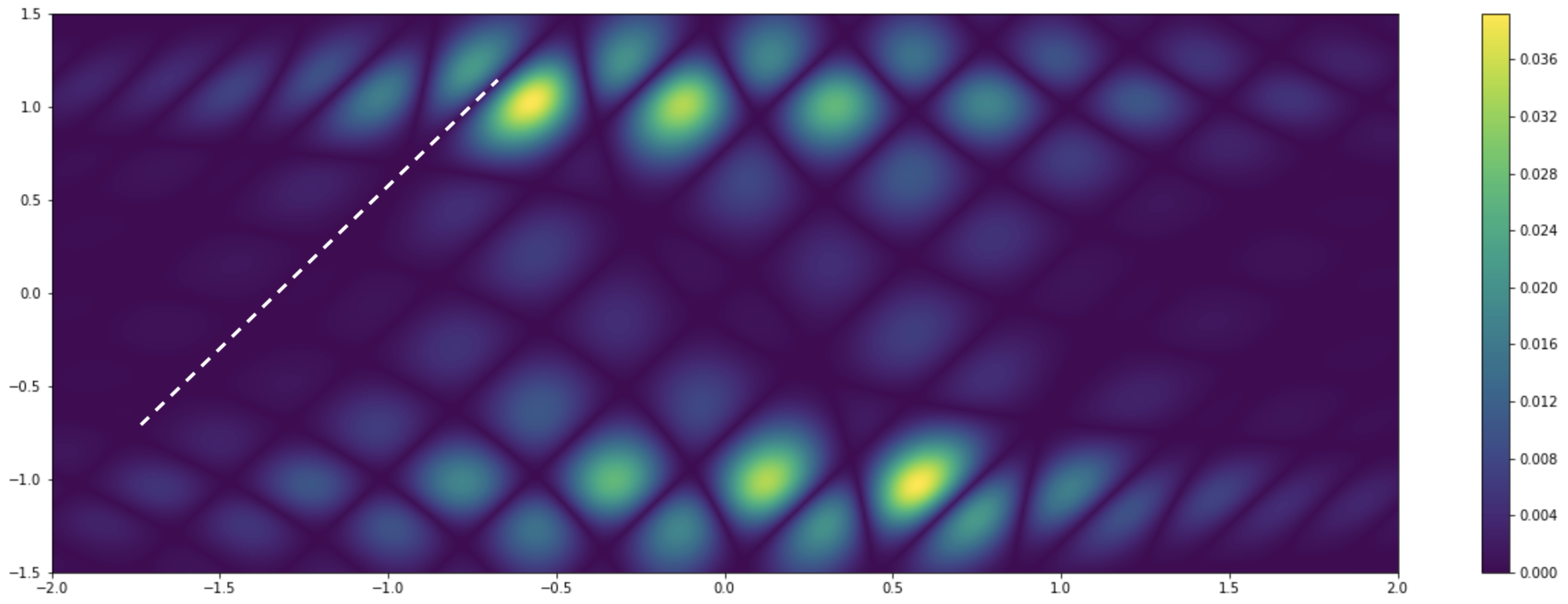
Figure 1. Plot of the pointwise distance QQ of the square of two spectrograms, Q≔||Vg​f1|2−|Vg​f2|2|Q\coloneqq||V_{g}f_{1}|^{2}-|V_{g}f_{2}|^{2}|, on the rectangle [−2,2]×[−1.5,1.5][-2,2]\times[-1.5,1.5] with window function g⁡(t)=e−|t|g(t)=e^{-|t|}. The functions f1f_{1} and f2f_{2} are chosen in such a way that QQ vanishes on parallel lines in the time-frequency plane, one of which is highlighted by the white dotted line. Such functions f1f_{1} and f2f_{2} can be obtained for every window function gg and they have the additional property that they do not agree up to a global phase. Their precise construction is the content of Section 3.

The conclusion of Theorem 1.3 is visualized in Figure 1. Prominent choices of window functions in Gabor analysis and its applications have the property that they are real-valued (Gaussians, Hermite functions, Airy disc functions, Hanning windows, rectangular windows). One could inquire about the question of whether a real-valuedness assumption on the underlying signal space achieves uniqueness from lattice samples, i.e. one specializes the considered input functions to belong to the space

L2​(ℝ,ℝ)={f∈L2​(ℝ):f​is real-valued}.L^{2}({\mathbb{R}},{\mathbb{R}})=\left\{f\in{L^{2}({\mathbb{R}})}:f\ \text{is real-valued}\right\}.

Under mild conditions on a lattice ℒ\mathcal{L}, the STFT phase retrieval problem still fails to be unique.

Theorem 1.4.

Let g∈L2​(ℝ,ℝ)g\in L^{2}({\mathbb{R}},{\mathbb{R}}) be a real-valued window function and ℒ=L​ℤ2\mathcal{L}=L{\mathbb{Z}}^{2} a lattice generated by

L=(abcd)∈GL2​(ℝ).L=\begin{pmatrix}a&b\\ c&d\end{pmatrix}\in\mathrm{GL}_{2}({\mathbb{R}}).

If aa and bb as well as cc and dd are linearly dependent over ℚ{\mathbb{Q}} then there exist two real-valued functions f1,f2∈L2​(ℝ,ℝ)f_{1},f_{2}\in L^{2}({\mathbb{R}},{\mathbb{R}}) which do not agree up to a global phase, f1≁f1f_{1}\nsim f_{1}, but their spectrograms agree on ℒ\mathcal{L},

|Vg​f1​(ℒ)|=|Vg​f2​(ℒ)|.|V_{g}f_{1}(\mathcal{L})|=|V_{g}f_{2}(\mathcal{L})|.

In particular, the conclusion of the previous theorem holds true if the generating matrix LL has rational entries, L∈GL2​(ℚ),L\in\mathrm{GL}_{2}({\mathbb{Q}}), or if the lattice is rectangular, i.e. ℒ=α​ℤ×β​ℤ\mathcal{L}=\alpha{\mathbb{Z}}\times\beta{\mathbb{Z}} for some α,β∈ℝ∖{0}\alpha,\beta\in{\mathbb{R}}\setminus\{0\}.

1.2. Outline

We quickly outline the structure of the paper. In Section 2 we define frequently used operators and their interrelations. Besides, we present the necessary background on the fractional Fourier transform and shift-invariant spaces. Based on this discussion we proceed in proving the main results of the article in Section 3. We conclude the article with Section 4, where we compare our results to previous work and outline a list of open problems suggested by the reported results.

2. Preliminaries on fractional Fourier transform and associated shift-invariant spaces

In this section, we collect several preliminary definitions and results about operators arising in time-frequency analysis, the fractional Fourier transform, and shift-invariant spaces.

2.1. Basic operations

The short-time Fourier transform of a function f∈L2​(ℝ)f\in{L^{2}({\mathbb{R}})} with respect to a window function g∈L2​(ℝ)g\in{L^{2}({\mathbb{R}})} is the map

Vg​f​(x,ω)=∫ℝf⁡(t)​g⁡(t−x)¯​e−2​π​i​ω​t​𝑑t,V_{g}f(x,\omega)=\int_{\mathbb{R}}f(t)\overline{g(t-x)}e^{-2\pi i\omega t}\,dt,

which is defined on the time-frequency plane ℝ2{\mathbb{R}}^{2}. This is a uniformly continuous map which measures the contribution to f⁡(t)f(t) of the frequency ω\omega near t=xt=x. In particular, it is pointwise defined. Hence, the STFT phase retrieval problem from lattice samples is well-defined. The so-called spectrogram of ff with respect to gg is the modulus of the STFT, i.e. the map

ℝ2→ℝ≥0,(x,ω)↦|Vg​f​(x,ω)|.{\mathbb{R}}^{2}\to{\mathbb{R}}_{\geq 0},\ \ (x,\omega)\mapsto|V_{g}f(x,\omega)|.

Note that Vg​f​(x,ω)V_{g}f(x,\omega) is the Fourier transform of f​g(⋅−x)¯f\overline{g(\cdot-x)} evaluated at ω\omega. The Fourier transform of a map u∈L1​(ℝ)u\in L^{1}({\mathbb{R}}) is given by

ℱ​u​(ω)≔u^​(ω)≔∫ℝu⁡(t)​e−2​π​i​ω​t​𝑑t.{\mathcal{F}}u(\omega)\coloneqq\hat{u}(\omega)\coloneqq\int_{\mathbb{R}}u(t)e^{-2\pi i\omega t}\,dt.

Recall that ℱ​u{\mathcal{F}}u is an element of C0​(ℝ)C_{0}({\mathbb{R}}), the Banach space of all continuous functions on the real line vanishing at infinity. The inverse Fourier transform is the map ℱ−1​u​(t)=ℱ​u​(−t){\mathcal{F}^{-1}}u(t)={\mathcal{F}}u(-t). The operator ℱ{\mathcal{F}} extends from L1​(ℝ)∩L2​(ℝ)L^{1}({\mathbb{R}})\cap{L^{2}({\mathbb{R}})} to a unitary operator mapping L2​(ℝ){L^{2}({\mathbb{R}})} bijectively onto L2​(ℝ){L^{2}({\mathbb{R}})}. In addition to the Fourier operator, we introduce some key-operations in time-frequency analysis. For τ,ν∈ℝ\tau,\nu\in{\mathbb{R}}, the translations operator Tτ:L2​(ℝ)→L2​(ℝ)T_{\tau}:{L^{2}({\mathbb{R}})}\to{L^{2}({\mathbb{R}})}, the modulation operator Mν:L2​(ℝ)→L2​(ℝ)M_{\nu}:{L^{2}({\mathbb{R}})}\to{L^{2}({\mathbb{R}})} and the reflection operator ℛ:L2​(ℝ)→L2​(ℝ)\mathcal{R}:{L^{2}({\mathbb{R}})}\to{L^{2}({\mathbb{R}})} are defined via

Tτ​f​(t)=f⁡(t−τ),Mν​f​(t)=e2​π​i​ν​t​f​(t),ℛ​f​(t)=f⁡(−t).\begin{split}T_{\tau}f(t)&=f(t-\tau),\\ M_{\nu}f(t)&=e^{2\pi i\nu t}f(t),\\ \mathcal{R}f(t)&=f(-t).\end{split}

Using translation and modulation, the short-time Fourier transform of ff with respect to gg simplifies to the expression Vg​f​(x,ω)=⟨f,Mω​Tx​g⟩V_{g}f(x,\omega)=\langle f,M_{\omega}T_{x}g\rangle where ⟨a,b⟩=∫ℝa⁡(t)​b⁡(t)¯​𝑑t\langle a,b\rangle=\int_{\mathbb{R}}a(t)\overline{b(t)}\,dt denotes the L2L^{2}-inner product of two functions a,b∈L2​(ℝ)a,b\in{L^{2}({\mathbb{R}})}. The next Lemma summarizes elementary relations between the operators ℱ,Vg,Tτ,Mν{\mathcal{F}},V_{g},T_{\tau},M_{\nu} and ℛ\mathcal{R} which will be used throughout the article. The simple proofs can be found, for instance, in [9, Chapter 1–3].

Lemma 2.1.

For every τ,ν,x,ω∈ℝ\tau,\nu,x,\omega\in{\mathbb{R}} and every f,g∈L2​(ℝ)f,g\in{L^{2}({\mathbb{R}})}, the operators defined above satisfy the relations

  1. (1)

    Tτ​Mν=e−2​π​i​τ​ν​Mν​TτT_{\tau}M_{\nu}=e^{-2\pi i\tau\nu}M_{\nu}T_{\tau}

  2. (2)

    ℱ​Tτ=M−τ​ℱ{\mathcal{F}}T_{\tau}=M_{-\tau}{\mathcal{F}}

  3. (3)

    ℱ−1​Tτ=Mτ​ℱ−1{\mathcal{F}^{-1}}T_{\tau}=M_{\tau}{\mathcal{F}^{-1}}

  4. (4)

    Tτ​ℛ=ℛ​T−τT_{\tau}\mathcal{R}=\mathcal{R}T_{-\tau}

  5. (5)

    ℱ​f¯=ℛ​ℱ​f¯\overline{{\mathcal{F}}f}=\mathcal{R}{\mathcal{F}}\overline{f}.

Moreover, the STFT satisfies the covariance property

  1. (6)

    Vg​(Tτ​Mν​f)​(x,ω)=e−2​π​i​τ​ω​Vg​f​(x−τ,ω−ν)V_{g}(T_{\tau}M_{\nu}f)(x,\omega)=e^{-2\pi i\tau\omega}V_{g}f(x-\tau,\omega-\nu).

2.2. Fractional Fourier transform

Denote by {Hn}n∈ℕ0\{H_{n}\}_{n\in{\mathbb{N}}_{0}} the Hermite basis functions on ℝ{\mathbb{R}}, defined by

Hn​(t)=21/4n!​(−12​π)n​eπ​t2​(dd​t)n​e−2​π​t2.H_{n}(t)=\frac{2^{1/4}}{\sqrt{n!}}\left(-\frac{1}{\sqrt{2\pi}}\right)^{n}e^{\pi t^{2}}\left(\frac{d}{dt}\right)^{n}e^{-2\pi t^{2}}.

The system {Hn}n∈ℕ0\{H_{n}\}_{n\in{\mathbb{N}}_{0}} constitutes and orthonormal basis for L2​(ℝ){L^{2}({\mathbb{R}})}. For θ∈ℝ\theta\in{\mathbb{R}}, the unitary operator ℱθ:L2​(ℝ)→L2​(ℝ){\mathcal{F}}_{\theta}:{L^{2}({\mathbb{R}})}\to{L^{2}({\mathbb{R}})},

ℱθ​f=∑n=0∞e−i​θ​n​⟨f,Hn⟩​Hn,{\mathcal{F}}_{\theta}f=\sum_{n=0}^{\infty}e^{-i\theta n}\langle f,H_{n}\rangle H_{n},

is called the fractional Fourier transform of order θ\theta. A detailed investigation of this transform and its appearance in quantum mechanics can be found in the early paper by Namias [19]. Besides, Namias’ article provides an alternative and frequently used definition of the operator ℱθ{\mathcal{F}}_{\theta} as an integral transform invoking chirp modulations [19, Section 3]. The following properties of the fractional Fourier transform are used throughout the present article [19, Section 4].

Lemma 2.2.

For every θ∈ℝ\theta\in{\mathbb{R}} and every ξ∈ℝ\xi\in{\mathbb{R}} the fractional Fourier transform ℱθ{\mathcal{F}}_{\theta} has the following properties:

  1. (1)

    ℱ0=Id,ℱπ2=ℱ,ℱ−π2=ℱ−1{\mathcal{F}}_{0}=\mathrm{Id},{\mathcal{F}}_{\frac{\pi}{2}}={\mathcal{F}},{\mathcal{F}}_{-\frac{\pi}{2}}={\mathcal{F}}^{-1} and ℱπ=ℛ{\mathcal{F}}_{\pi}=\mathcal{R}

  2. (2)

    ℱθ+ξ=ℱθ​ℱξ{\mathcal{F}}_{\theta+\xi}={\mathcal{F}}_{\theta}{\mathcal{F}}_{\xi}

  3. (3)

    ℱθ{\mathcal{F}}_{\theta} commutes with ℛ\mathcal{R}

  4. (4)

    If f∈L2​(ℝ)f\in{L^{2}({\mathbb{R}})} then ℱθ​f¯=ℱ−θ​f¯\overline{{\mathcal{F}}_{\theta}f}={\mathcal{F}}_{-\theta}\overline{f}

In the context of time-frequency analysis, the perhaps most significant property of the operator ℱθ{\mathcal{F}}_{\theta} is its relation to rotations in the time-frequency plane [16, 18]. To present the precise mathematical formulation of this fact, we define for θ∈ℝ\theta\in{\mathbb{R}} the rotation matrix Rθ∈ℝ2×2R_{\theta}\in{\mathbb{R}}^{2\times 2} via

(2) Rθ=(cos⁡θ−sin⁡θsin⁡θcos⁡θ).R_{\theta}=\begin{pmatrix}\cos\theta&-\sin\theta\\ \sin\theta&\cos\theta\end{pmatrix}.

The rotation property of the fractional Fourier transform reads as follows.

Theorem 2.3.

If RθR_{\theta} denotes the rotation matrix as given in equation (2) then for every f,g∈L2​(ℝ)f,g\in{L^{2}({\mathbb{R}})} and every (x,ω)∈ℝ2(x,\omega)\in{\mathbb{R}}^{2} one has

Vg​f​(Rθ​(x,ω))=e−π​i​q​(θ)​eπ​i​x​ω​Vℱθ​g​(ℱθ​f)​(x,ω)V_{g}f(R_{\theta}(x,\omega))=e^{-\pi iq(\theta)}e^{\pi ix\omega}V_{{\mathcal{F}}_{\theta}g}({\mathcal{F}}_{\theta}f)(x,\omega)

with q⁡(θ)=(x​cos⁡θ−ω​sin⁡θ)​(x​sin⁡θ+ω​cos⁡θ)q(\theta)=(x\cos\theta-\omega\sin\theta)(x\sin\theta+\omega\cos\theta).

A proof of Theorem 2.3 can be found in [3]. Moreover, the reader may consult [16, Section 3.4] for a discussion of the rotation property. The phase retrievability of functions f∈L2​(ℝ)f\in{L^{2}({\mathbb{R}})} from measurements of the form {|ℱθ​f|:θ∈Θ}\{|{\mathcal{F}}_{\theta}f|:\theta\in\Theta\}, with Θ⊂ℝ\Theta\subset{\mathbb{R}} constituting a set of orders, was studied by Jaming [16] and Carmeli et al. [6].

2.3. Shift-invariant spaces

In this section, we shall discuss shift-invariant spaces, both in the classical sense as well as generalizations in the context of fractional Fourier transform. We start by introducing classical shift-invariant spaces. Consider a generating function u∈L2​(ℝ)u\in{L^{2}({\mathbb{R}})} and a constant 𝔰>0{\mathfrak{s}}>0. The subspace 𝒱𝔰​(u)⊂L2​(ℝ)\mathcal{V}_{\mathfrak{s}}(u)\subset{L^{2}({\mathbb{R}})}, defined as the L2L^{2}-closure of the 𝔰​ℤ{\mathfrak{s}}{\mathbb{Z}}-shifts of uu,

(3) 𝒱𝔰(u)≔span⁡{T𝔰​k​u:k∈ℤ}¯,\mathcal{V}_{\mathfrak{s}}(u)\coloneqq\overline{{\mathrm{span}}\left\{T_{{\mathfrak{s}}k}u:k\in{\mathbb{Z}}\right\}},

is called the (principle) shift-invariant space generated by uu and step-size 𝔰>0{\mathfrak{s}}>0. Shift-invariance means that whenever h∈𝒱𝔰​(u)h\in\mathcal{V}_{\mathfrak{s}}(u), so is T𝔰​n​hT_{{\mathfrak{s}}n}h for every n∈ℤn\in{\mathbb{Z}}. A characterization of functions belonging to 𝒱𝔰​(u)\mathcal{V}_{\mathfrak{s}}(u) was given in [8]. If h∈𝒱𝔰​(u)h\in\mathcal{V}_{\mathfrak{s}}(u) is such that hh has a representation of the form h=∑k∈ℤck​T𝔰​k​uh=\sum_{k\in{\mathbb{Z}}}c_{k}T_{{\mathfrak{s}}k}u for some sequence {ck}⊂ℂ\{c_{k}\}\subset{\mathbb{C}} then we call {ck}\{c_{k}\} a defining sequence of hh. If {ck}\{c_{k}\} belongs to the space c00​(ℤ)c_{00}({\mathbb{Z}}) of sequences with only finitely many nonzero components then clearly ∑k∈ℤck​T𝔰​k​u\sum_{k\in{\mathbb{Z}}}c_{k}T_{{\mathfrak{s}}k}u is a well-defined function in 𝒱𝔰​(u)\mathcal{V}_{\mathfrak{s}}(u) and no convergence issues appear. Care should be taken if {ck}∉c00​(ℤ)\{c_{k}\}\notin c_{00}({\mathbb{Z}}): since we did not make any additional assumptions on the generating function u∈L2​(ℝ)u\in{L^{2}({\mathbb{R}})} (in particular, we are not assuming that {T𝔰​k​u:k∈ℤ}\{T_{{\mathfrak{s}}k}u:k\in{\mathbb{Z}}\} is a Riesz basis or frame for 𝒱𝔰​(u)\mathcal{V}_{\mathfrak{s}}(u)), we may not be able to represent every function f∈𝒱𝔰​(u)f\in\mathcal{V}_{\mathfrak{s}}(u) in the form ∑k∈ℤck​T𝔰​k​u\sum_{k\in{\mathbb{Z}}}c_{k}T_{{\mathfrak{s}}k}u. An assumption which guarantees unconditional convergence for every square-summable sequence {ck}∈ℓ2​(ℤ)\{c_{k}\}\in\ell^{2}({\mathbb{Z}}) is the requirement that {T𝔰​k​u:k∈ℤ}\{T_{{\mathfrak{s}}k}u:k\in{\mathbb{Z}}\} is a Bessel sequence [7, Corollary 3.2.5]. Recall that a sequence {xk}\{x_{k}\} in a Hilbert space HH is a Bessel sequence if

∀x∈H:∑k∈ℤ|⟨x,xk⟩|2<∞.\forall x\in H:\sum_{k\in{\mathbb{Z}}}|\langle x,x_{k}\rangle|^{2}<\infty.
Theorem 2.4.

If {xk:k∈ℤ}\{x_{k}:k\in{\mathbb{Z}}\} is a Bessel sequence in a Hilbert space HH then for every {ck}∈ℓ2​(ℤ)\{c_{k}\}\in\ell^{2}({\mathbb{Z}}) the series ∑k∈ℤck​xk\sum_{k\in{\mathbb{Z}}}c_{k}x_{k} converges unconditionally in HH.

If one would apply the Fourier transform to 𝒱𝔰​(u)\mathcal{V}_{\mathfrak{s}}(u) then the resulting space

ℳ𝔰​(u)={ℱ​h:h∈𝒱𝔰​(u)}\mathcal{M}_{\mathfrak{s}}(u)=\left\{{\mathcal{F}}h:h\in\mathcal{V}_{\mathfrak{s}}(u)\right\}

is modulation invariant (or: invariant under a Fourier shift), i.e. M𝔰​n​h∈ℳ𝔰​(u)M_{{\mathfrak{s}}n}h\in\mathcal{M}_{\mathfrak{s}}(u) for every n∈ℤn\in{\mathbb{Z}} provided that h∈ℳ𝔰​(u)h\in\mathcal{M}_{\mathfrak{s}}(u). Now observe that

T𝔰​k=Id​T𝔰​k​Id,M𝔰​k=ℱ−1​T𝔰​k​ℱ,T_{{\mathfrak{s}}k}=\mathrm{Id}\,T_{{\mathfrak{s}}k}\,\mathrm{Id},\ \ M_{{\mathfrak{s}}k}={\mathcal{F}}^{-1}T_{{\mathfrak{s}}k}{\mathcal{F}},

or, in the language of fractional Fourier transform,

T𝔰​k=ℱ0​T𝔰​k​ℱ0,M𝔰​k=ℱ−π2​T𝔰​k​ℱπ2.T_{{\mathfrak{s}}k}={\mathcal{F}}_{0}T_{{\mathfrak{s}}k}{\mathcal{F}}_{0},\ \ M_{{\mathfrak{s}}k}={\mathcal{F}}_{-\frac{\pi}{2}}T_{{\mathfrak{s}}k}{\mathcal{F}}_{\frac{\pi}{2}}.

The previous identities motivate the definition of a fractional Fourier shift.

Definition 2.5.

Let τ,θ∈ℝ\tau,\theta\in{\mathbb{R}}. The operator TτθT_{\tau}^{\theta}, defined by

Tτθ≔ℱ−θ​Tτ​ℱθT_{\tau}^{\theta}\coloneqq{\mathcal{F}}_{-\theta}T_{\tau}{\mathcal{F}}_{\theta}

is called the fractional Fourier shift by τ\tau of order θ\theta.

We have Tτ0=TτT_{\tau}^{0}=T_{\tau} and Tτπ2=MτT_{\tau}^{\frac{\pi}{2}}=M_{\tau}. Hence, the operator TτθT_{\tau}^{\theta} interpolates between the ordinary shift and the modulation, i.e. a Fourier shift. In a natural way, the fractional Fourier shift extends the concept of classical shift-invariant spaces.

Definition 2.6.

Let u∈L2​(ℝ)u\in{L^{2}({\mathbb{R}})} be a generating function and 𝔰>0{\mathfrak{s}}>0. The space

𝒱𝔰θ(u)≔span⁡{T𝔰​kθ​u:k∈ℤ}¯\mathcal{V}_{\mathfrak{s}}^{\theta}(u)\coloneqq\overline{{\mathrm{span}}\left\{T_{{\mathfrak{s}}k}^{\theta}u:k\in{\mathbb{Z}}\right\}}

is called the shift-invariant space associated to the fractional Fourier shift generated by uu and step-size 𝔰>0{\mathfrak{s}}>0. In the case θ=0\theta=0 we have 𝒱𝔰0​(u)=𝒱𝔰​(u)\mathcal{V}_{\mathfrak{s}}^{0}(u)=\mathcal{V}_{\mathfrak{s}}(u) with 𝒱𝔰​(u)\mathcal{V}_{\mathfrak{s}}(u) being defined as in (3).

For details and properties on shift-invariant spaces associated to the fractional Fourier shift, the reader may consult the article [4] and the references therein. A direct application of Theorem 2.4 gives the following statement.

Corollary 2.7.

Let u∈L2​(ℝ)u\in{L^{2}({\mathbb{R}})} be a generating function, 𝔰>0{\mathfrak{s}}>0 a step-size and θ∈ℝ\theta\in{\mathbb{R}} an order. If the system of fractional Fourier shifts {T𝔰​kθ​u:k∈ℤ}\{T_{{\mathfrak{s}}k}^{\theta}u:k\in{\mathbb{Z}}\} constitutes a Bessel sequence in L2​(ℝ){L^{2}({\mathbb{R}})} then for every {ck}∈ℓ2​(ℤ)\{c_{k}\}\in\ell^{2}({\mathbb{Z}}) the series ∑k∈ℤck​T𝔰​kθ​u\sum_{k\in{\mathbb{Z}}}c_{k}T_{{\mathfrak{s}}k}^{\theta}u converges unconditionally to an element in 𝒱𝔰θ​(u)\mathcal{V}_{\mathfrak{s}}^{\theta}(u).

3. Main results

In this section, we present and prove the main results of the paper. We derive functions f1,f2∈L2​(ℝ)f_{1},f_{2}\in{L^{2}({\mathbb{R}})} which have the property that their spectrograms agree on certain selected subsets of the time-frequency plane. Moreover, we discuss under which assumptions such functions do not agree up to a global phase and which conditions imply that they can be chosen to be real-valued.

3.1. Identical spectrograms and non-equivalence conditions

Let u∈L2​(ℝ),𝔰>0u\in{L^{2}({\mathbb{R}})},{\mathfrak{s}}>0 and θ∈ℝ\theta\in{\mathbb{R}}. In the sequel we shall fix the following notation: whenever f∈𝒱𝔰θ​(u)f\in\mathcal{V}_{\mathfrak{s}}^{\theta}(u) has a representation of the form f=∑k∈ℤck​T𝔰​kθ​uf=\sum_{k\in{\mathbb{Z}}}c_{k}T_{{\mathfrak{s}}k}^{\theta}u with a defining sequence {ck}⊂ℂ\{c_{k}\}\subset{\mathbb{C}} then the map f×f_{\times} is defined by

f×≔∑k∈ℤck¯​T𝔰​kθ​u,f_{\times}\coloneqq\sum_{k\in{\mathbb{Z}}}\overline{c_{k}}T_{{\mathfrak{s}}k}^{\theta}u,

i.e. f×f_{\times} arises from ff via complex conjugation of the defining sequence {ck}\{c_{k}\}. We now show that a suitable choice of the generator uu implies equality of the spectrogram of ff and f×f_{\times} on parallel lines of the form

(4) Rθ(ℝ×hℤ)≔{(cos⁡θ−sin⁡θsin⁡θcos⁡θ)(xω):x∈ℝ,ω∈hℤ},h>0.R_{\theta}({\mathbb{R}}\times h{\mathbb{Z}})\coloneqq\left\{\begin{pmatrix}\cos\theta&-\sin\theta\\ \sin\theta&\cos\theta\end{pmatrix}\begin{pmatrix}x\\ \omega\end{pmatrix}:x\in{\mathbb{R}},\,\omega\in h{\mathbb{Z}}\right\},\ \ h>0.
Theorem 3.1.

Let g∈L2​(ℝ)g\in{L^{2}({\mathbb{R}})} be a window function, 𝔰>0{\mathfrak{s}}>0 a step-size and θ∈ℝ\theta\in{\mathbb{R}} an order. If f∈𝒱𝔰θ​(ℛ​g)f\in\mathcal{V}_{\mathfrak{s}}^{\theta}(\mathcal{R}g) has defining sequence {ck}∈c00​(ℤ)\{c_{k}\}\in c_{00}({\mathbb{Z}}) then

|Vg​f​(Rθ​(ℝ×1𝔰​ℤ))|=|Vg​(f×)​(Rθ​(ℝ×1𝔰​ℤ))|.|V_{g}f(R_{\theta}({\mathbb{R}}\times\tfrac{1}{{\mathfrak{s}}}{\mathbb{Z}}))|=|V_{g}(f_{\times})(R_{\theta}({\mathbb{R}}\times\tfrac{1}{{\mathfrak{s}}}{\mathbb{Z}}))|.

If, in addition, the system {T𝔰​kθ​(ℛ​g):k∈ℤ}\{T_{{\mathfrak{s}}k}^{\theta}(\mathcal{R}g):k\in{\mathbb{Z}}\} is a Bessel sequence then the same conclusion holds true, provided that ff has defining sequence {ck}∈ℓ2​(ℤ)\{c_{k}\}\in\ell^{2}({\mathbb{Z}}).

Proof.

Let (x,ω)∈ℝ2(x,\omega)\in{\mathbb{R}}^{2} and let RθR_{\theta} be the rotation matrix as defined in equation (2). Suppose that f∈𝒱𝔰θ​(ℛ​g)f\in\mathcal{V}_{\mathfrak{s}}^{\theta}(\mathcal{R}g) has defining sequence {ck}∈c00​(ℤ)\{c_{k}\}\in c_{00}({\mathbb{Z}}). Invoking the definition of the fractional Fourier shift, ff can be written as

f=ℱ−θ​∑k∈ℤck​T𝔰​k​ℱθ​ℛ​g.f={\mathcal{F}}_{-\theta}\sum_{k\in{\mathbb{Z}}}c_{k}T_{{\mathfrak{s}}k}{\mathcal{F}}_{\theta}\mathcal{R}g.

We now evaluate the spectrogram of ff with respect to the window function gg at a θ\theta-rotation of (x,ω)(x,\omega). Consulting the properties of the fractional Fourier transform as presented in Lemma 2.2 yields

|Vg​f​(Rθ​(x,ω))|\displaystyle|V_{g}f(R_{\theta}(x,\omega))| =Theorem 2.3|Vℱθ​g​(∑k∈ℤck​T𝔰​k​ℱθ​ℛ​g)​(x,ω)|\displaystyle\mathrel{\overset{\scriptsize{\makebox[47.38907pt][c]{Theorem \ref{thm:frac_rotation}}}}{=}}\left|V_{{\mathcal{F}}_{\theta}g}\left(\sum_{k\in{\mathbb{Z}}}c_{k}T_{{\mathfrak{s}}k}{\mathcal{F}}_{\theta}\mathcal{R}g\right)(x,\omega)\right|
=linearity|∑k∈ℤck​Vℱθ​g​(T𝔰​k​ℱθ​ℛ​g)​(x,ω)|\displaystyle\mathrel{\overset{\scriptsize{\makebox[47.38907pt][c]{linearity}}}{=}}\left|\sum_{k\in{\mathbb{Z}}}c_{k}V_{{\mathcal{F}}_{\theta}g}(T_{{\mathfrak{s}}k}{\mathcal{F}}_{\theta}\mathcal{R}g)(x,\omega)\right|
=Lemma 2.1(6)|∑k∈ℤck​e−2​π​i​𝔰​k​ω​Vℱθ​g​(ℱθ​ℛ​g)​(x−𝔰​k,ω)|\displaystyle\mathrel{\overset{\scriptsize{\makebox[52.33353pt][c]{Lemma \ref{lemma:comm_relations}(6)}}}{=}}\left|\sum_{k\in{\mathbb{Z}}}c_{k}e^{-2\pi i{\mathfrak{s}}k\omega}V_{{\mathcal{F}}_{\theta}g}({\mathcal{F}}_{\theta}\mathcal{R}g)(x-{\mathfrak{s}}k,\omega)\right|
=|∑k∈ℤck​e−2​π​i​𝔰​k​ω​ℱ​((ℱθ​ℛ​g)​(Tx−𝔰​k​ℱθ​g¯))​(ω)|\displaystyle\mathrel{\overset{\scriptsize{\makebox[52.33353pt][c]{}}}{=}}\left|\sum_{k\in{\mathbb{Z}}}c_{k}e^{-2\pi i{\mathfrak{s}}k\omega}{\mathcal{F}}\left(({\mathcal{F}}_{\theta}\mathcal{R}g)(\overline{T_{x-{\mathfrak{s}}k}{\mathcal{F}}_{\theta}g})\right)(\omega)\right|
=Lemma 2.2(4)|∑k∈ℤck​e−2​π​i​𝔰​k​ω​ℱ​((ℱθ​ℛ​g)​(Tx−𝔰​k​ℱ−θ​g¯))​(ω)|.\displaystyle\mathrel{\overset{\scriptsize{\makebox[52.33353pt][c]{Lemma \ref{lemma:fracft_properties}(4)}}}{=}}\left|\sum_{k\in{\mathbb{Z}}}c_{k}e^{-2\pi i{\mathfrak{s}}k\omega}{\mathcal{F}}\left(({\mathcal{F}}_{\theta}\mathcal{R}g)(T_{x-{\mathfrak{s}}k}{\mathcal{F}}_{-\theta}\overline{g})\right)(\omega)\right|.

We continue by inspecting the spectrogram of f×f_{\times}. Replacing ckc_{k} with ck¯\overline{c_{k}} in equation (3.1) shows that the spectrogram of f×f_{\times} satisfies

|Vg​(f×)​(Rθ​(x,ω))|\displaystyle|V_{g}(f_{\times})(R_{\theta}(x,\omega))| =|∑k∈ℤck¯​e−2​π​i​𝔰​k​ω​ℱ​((ℱθ​ℛ​g)​(Tx−𝔰​k​ℱ−θ​g¯))​(ω)|\displaystyle\mathrel{\overset{\scriptsize{\makebox[52.33353pt][c]{}}}{=}}\left|\sum_{k\in{\mathbb{Z}}}\overline{c_{k}}e^{-2\pi i{\mathfrak{s}}k\omega}{\mathcal{F}}\left(({\mathcal{F}}_{\theta}\mathcal{R}g)(T_{x-{\mathfrak{s}}k}{\mathcal{F}}_{-\theta}\overline{g})\right)(\omega)\right|
=|∑k∈ℤck​e2​π​i​𝔰​k​ω​ℱ⁡((ℱθ​ℛ​g)​(Tx−𝔰​k​ℱ−θ​g¯))​(ω)¯|\displaystyle\mathrel{\overset{\scriptsize{\makebox[52.33353pt][c]{}}}{=}}\left|\sum_{k\in{\mathbb{Z}}}c_{k}e^{2\pi i{\mathfrak{s}}k\omega}\overline{{\mathcal{F}}\left(({\mathcal{F}}_{\theta}\mathcal{R}g)(T_{x-{\mathfrak{s}}k}{\mathcal{F}}_{-\theta}\overline{g})\right)(\omega)}\right|
=Lemma 2.1(5)|∑k∈ℤck​e2​π​i​𝔰​k​ω​ℛ​ℱ​((ℱθ​ℛ​g)​(Tx−𝔰​k​ℱ−θ​g¯)¯)​(ω)|\displaystyle\mathrel{\overset{\scriptsize{\makebox[52.33353pt][c]{Lemma \ref{lemma:comm_relations}(5)}}}{=}}\left|\sum_{k\in{\mathbb{Z}}}c_{k}e^{2\pi i{\mathfrak{s}}k\omega}\mathcal{R}{\mathcal{F}}\left(\overline{({\mathcal{F}}_{\theta}\mathcal{R}g)(T_{x-{\mathfrak{s}}k}{\mathcal{F}}_{-\theta}\overline{g})}\right)(\omega)\right|
=Lemma 2.2(4)|∑k∈ℤck​e2​π​i​𝔰​k​ω​ℛ​ℱ​((ℱ−θ​ℛ​g¯)​(Tx−𝔰​k​ℱθ​g))​(ω)|\displaystyle\mathrel{\overset{\scriptsize{\makebox[52.33353pt][c]{Lemma \ref{lemma:fracft_properties}(4)}}}{=}}\left|\sum_{k\in{\mathbb{Z}}}c_{k}e^{2\pi i{\mathfrak{s}}k\omega}\mathcal{R}{\mathcal{F}}\left(({\mathcal{F}}_{-\theta}\mathcal{R}\overline{g})(T_{x-{\mathfrak{s}}k}{\mathcal{F}}_{\theta}g)\right)(\omega)\right|
=Lemma 2.2(3)|∑k∈ℤck​e2​π​i​𝔰​k​ω​ℱ​(ℛ⁡[(ℱ−θ​ℛ​g¯)​(Tx−𝔰​k​ℱθ​g)])​(ω)|\displaystyle\mathrel{\overset{\scriptsize{\makebox[52.33353pt][c]{Lemma \ref{lemma:fracft_properties}(3)}}}{=}}\left|\sum_{k\in{\mathbb{Z}}}c_{k}e^{2\pi i{\mathfrak{s}}k\omega}{\mathcal{F}}\left(\mathcal{R}[({\mathcal{F}}_{-\theta}\mathcal{R}\overline{g})(T_{x-{\mathfrak{s}}k}{\mathcal{F}}_{\theta}g)]\right)(\omega)\right|
=Lemma 2.2(3)|∑k∈ℤck​e2​π​i​𝔰​k​ω​ℱ​((ℱ−θ​g¯)​(T𝔰​k−x​ℱθ​ℛ​g))​(ω)|\displaystyle\mathrel{\overset{\scriptsize{\makebox[52.33353pt][c]{Lemma \ref{lemma:fracft_properties}(3)}}}{=}}\left|\sum_{k\in{\mathbb{Z}}}c_{k}e^{2\pi i{\mathfrak{s}}k\omega}{\mathcal{F}}\left(({\mathcal{F}}_{-\theta}\overline{g})(T_{{\mathfrak{s}}k-x}{\mathcal{F}}_{\theta}\mathcal{R}g)\right)(\omega)\right|
=Lemma 2.1(2)|∑k∈ℤck​e2​π​i​𝔰​k​ω​e−2​π​i​ω​(𝔰​k−x)​ℱ​((Tx−𝔰​k​ℱ−θ​g¯)​(ℱθ​ℛ​g))​(ω)|\displaystyle\mathrel{\overset{\scriptsize{\makebox[52.33353pt][c]{Lemma \ref{lemma:comm_relations}(2)}}}{=}}\left|\sum_{k\in{\mathbb{Z}}}c_{k}e^{2\pi i{\mathfrak{s}}k\omega}e^{-2\pi i\omega({\mathfrak{s}}k-x)}{\mathcal{F}}\left((T_{x-{\mathfrak{s}}k}{\mathcal{F}}_{-\theta}\overline{g})({\mathcal{F}}_{\theta}\mathcal{R}g)\right)(\omega)\right|
=|∑k∈ℤck​ℱ​((Tx−𝔰​k​ℱ−θ​g¯)​(ℱθ​ℛ​g))​(ω)|.\displaystyle\mathrel{\overset{\scriptsize{\makebox[52.33353pt][c]{}}}{=}}\left|\sum_{k\in{\mathbb{Z}}}c_{k}{\mathcal{F}}\left((T_{x-{\mathfrak{s}}k}{\mathcal{F}}_{-\theta}\overline{g})({\mathcal{F}}_{\theta}\mathcal{R}g)\right)(\omega)\right|.

Now let ω=n𝔰\omega=\frac{n}{{\mathfrak{s}}} for some n∈ℤn\in{\mathbb{Z}}. In this case, the term e−2​π​i​𝔰​k​ωe^{-2\pi i{\mathfrak{s}}k\omega} appearing in the equation (3.1) simplifies to e−2​π​i​𝔰​k​ω=e−2​π​i​k​n=1e^{-2\pi i{\mathfrak{s}}k\omega}=e^{-2\pi ikn}=1. This shows that |Vg​f​(Rθ​(x,n𝔰))|=|Vg​(f×)​(Rθ​(x,n𝔰))||V_{g}f(R_{\theta}(x,\tfrac{n}{{\mathfrak{s}}}))|=|V_{g}(f_{\times})(R_{\theta}(x,\tfrac{n}{{\mathfrak{s}}}))| for every n∈ℤn\in{\mathbb{Z}}. Since x∈ℝx\in{\mathbb{R}} was arbitrary, we obtain the desired equality of the two spectrograms on the parallel lines Rθ​(ℝ×1𝔰​ℤ)R_{\theta}({\mathbb{R}}\times\tfrac{1}{{\mathfrak{s}}}{\mathbb{Z}}). Under the additional assumption that the system {T𝔰​kθ​(ℛ​g):k∈ℤ}\{T_{{\mathfrak{s}}k}^{\theta}(\mathcal{R}g):k\in{\mathbb{Z}}\} forms a Bessel sequence, Corollary 2.7 implies that for every {ck}∈ℓ2​(ℤ)\{c_{k}\}\in\ell^{2}({\mathbb{Z}}) the series ∑k∈ℤck​T𝔰​k​ℛ​g\sum_{k\in{\mathbb{Z}}}c_{k}T_{{\mathfrak{s}}k}\mathcal{R}g converges unconditionally in L2​(ℝ){L^{2}({\mathbb{R}})}. Since {ck¯}∈ℓ2​(ℤ)\{\overline{c_{k}}\}\in\ell^{2}({\mathbb{Z}}) if and only if {ck}∈ℓ2​(ℤ)\{c_{k}\}\in\ell^{2}({\mathbb{Z}}), the same holds for the series ∑k∈ℤck¯​T𝔰​k​ℛ​g\sum_{k\in{\mathbb{Z}}}\overline{c_{k}}T_{{\mathfrak{s}}k}\mathcal{R}g. By continuity and linearity of the fractional Fourier transform, the exact same argument as above implies equality of the spectrogram of ff and f×f_{\times} on Rθ​(ℝ×1𝔰​ℤ)R_{\theta}({\mathbb{R}}\times\tfrac{1}{{\mathfrak{s}}}{\mathbb{Z}}). ∎

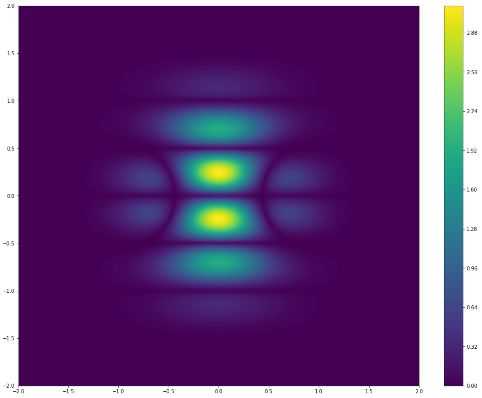
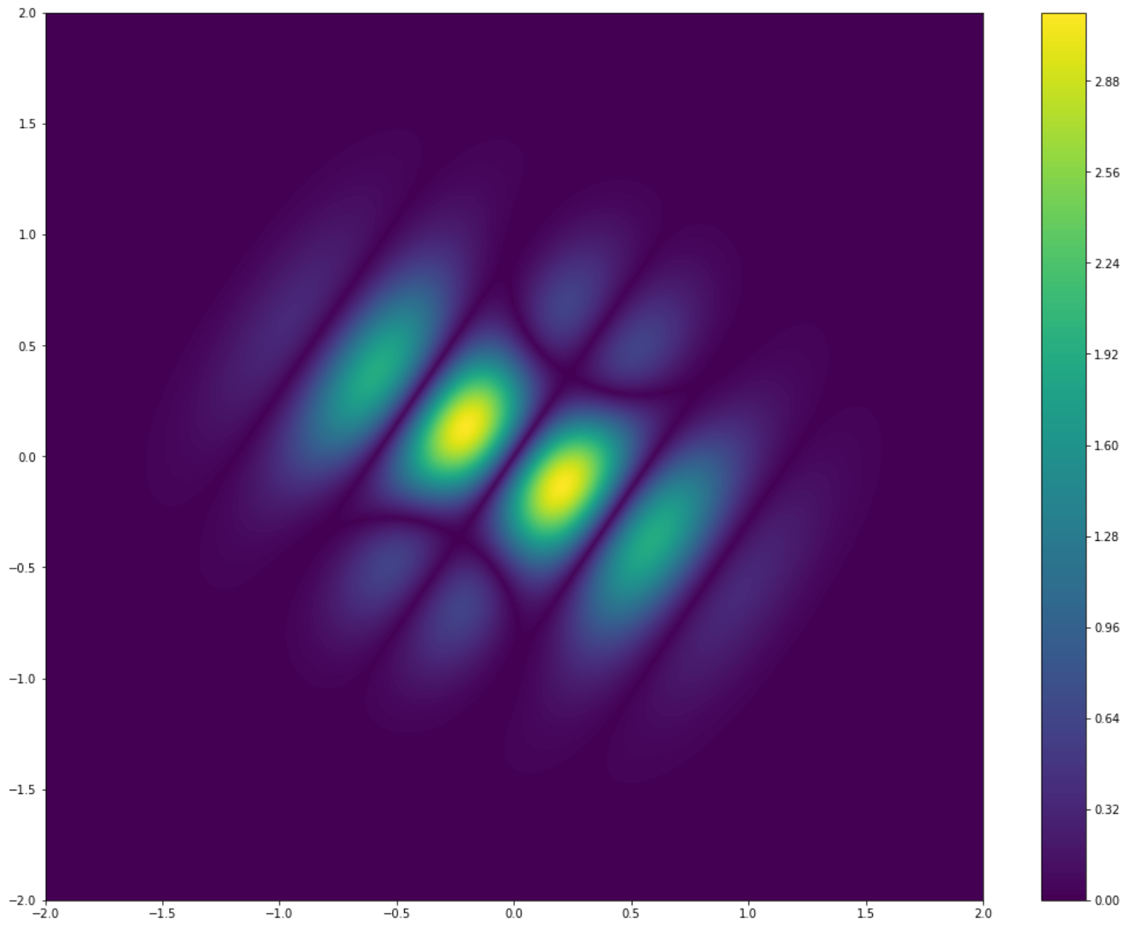
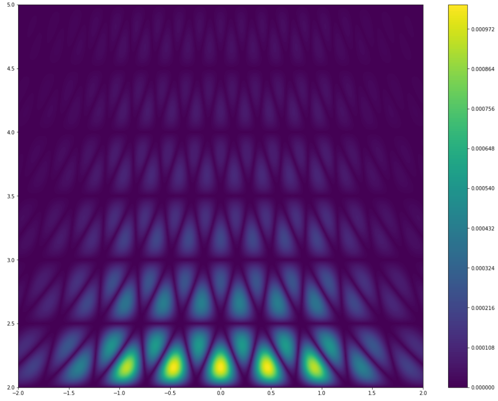
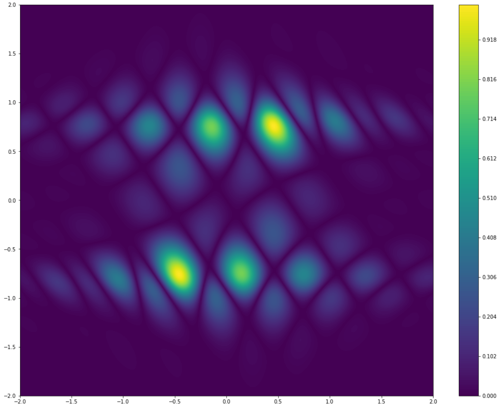
The statement obtained in Theorem 3.1 is visualized in Figure 2 and Figure 3. The functions ff and f×f_{\times} defined in Theorem 3.1 constitute candidates of functions for which their spectrograms agree on parallel lines whereas the functions themselves might not agree up to a global phase. We now examine criteria on the defining sequence {ck}\{c_{k}\} of ff so that ff and f×f_{\times} do not agree up to a global phase. Before doing so, we recall the concept of ω\omega-independence [24, p. 34].

Definition 3.2.

A sequence {xn}n∈ℤ\{x_{n}\}_{n\in{\mathbb{Z}}} of elements in a Banach space XX is said to be ω\omega-independent if the equality

(15) ∑n∈ℤcn​xn=0\sum_{n\in{\mathbb{Z}}}c_{n}x_{n}=0

is possible only for cn=0,n∈ℤc_{n}=0,n\in{\mathbb{Z}}.

Recall that in the definition of a linearly independent system, the norm-convergent series in (15) is replaced by a finite sum. Systems of translates of a function which constitute an ω\omega-independent sequence were studied in [23]. We continue by introducing a class of sequences which obeys a geometric property.

Definition 3.3.

The subset ℓ𝒪2​(ℤ)⊂ℓ2​(ℤ)\ell^{2}_{\mathcal{O}}({\mathbb{Z}})\subset\ell^{2}({\mathbb{Z}}) of square-summable sequences whose elements do not lie on a line in the complex plane passing through the origin is defined as

ℓ𝒪2(ℤ)≔{{ck}∈ℓ2(ℤ):∄α∈ℝs.t.{ck}⊂ei​αℝ}.\ell^{2}_{\mathcal{O}}({\mathbb{Z}})\coloneqq\left\{\{c_{k}\}\in\ell^{2}({\mathbb{Z}}):\nexists\,\alpha\in{\mathbb{R}}\ \mathrm{s.t.}\ \{c_{k}\}\subset e^{i\alpha}{\mathbb{R}}\right\}.

Note that ℓ𝒪2​(ℤ)\ell^{2}_{\mathcal{O}}({\mathbb{Z}}) is invariant under complex conjugation, i.e. {ck}∈ℓ𝒪2​(ℤ)\{c_{k}\}\in\ell^{2}_{\mathcal{O}}({\mathbb{Z}}) if and only if {ck¯}∈ℓ𝒪2​(ℤ)\{\overline{c_{k}}\}\in\ell^{2}_{\mathcal{O}}({\mathbb{Z}}). In order to show that sequences in ℓ𝒪2​(ℤ)\ell^{2}_{\mathcal{O}}({\mathbb{Z}}) produce functions ff and f×f_{\times} which do not agree up to a global phase, we make use of the following simple observation.

Lemma 3.4.

Let YY be an arbitrary set and f:Y→ℂf:Y\to{\mathbb{C}} a complex-valued map. Then f∼f¯f\sim\overline{f} if and only if there exists an α∈ℝ\alpha\in{\mathbb{R}} such that f⁡(y)∈ei​α​ℝf(y)\in e^{i\alpha}{\mathbb{R}} for every y∈Yy\in Y.

Proof.

We first prove the sufficiency of the property f∼f¯f\sim\overline{f}. To this end, let ν∈ℝ\nu\in{\mathbb{R}} such that f⁡(y)=ei​ν​f⁡(y)¯f(y)=e^{i\nu}\overline{f(y)} for every y∈Yy\in Y. Let f⁡(y)=ei​ϕ​(y)​|f⁡(y)|f(y)=e^{i\phi(y)}|f(y)| and f⁡(y)¯=e−i​ϕ​(y)​|f⁡(y)|\overline{f(y)}=e^{-i\phi(y)}|f(y)| with ϕ\phi being a phase function corresponding to ff. Let Λ={y∈Y:f⁡(y)≠0}\Lambda=\{y\in Y:f(y)\neq 0\}. It follows that

ei⁡(2​ϕ​(y)−ν)=1e^{i(2\phi(y)-\nu)}=1

for every y∈Λy\in\Lambda which implies that there exists an n⁡(y)∈ℤn(y)\in{\mathbb{Z}} so that ϕ⁡(y)=π​n​(y)+ν2\phi(y)=\pi n(y)+\tfrac{\nu}{2}. Thus,

f⁡(y)=ei​π​n​(y)​ei​ν2​|f⁡(y)|=ei​ν2​((−1)n⁡(y)​|f⁡(y)|)f(y)=e^{i\pi n(y)}e^{i\frac{\nu}{2}}|f(y)|=e^{i\frac{\nu}{2}}\left((-1)^{n(y)}|f(y)|\right)

which shows that ff takes values on the line ei​ν2​ℝe^{i\frac{\nu}{2}}{\mathbb{R}}. Conversely, suppose that ff takes values on a line ei​α​ℝe^{i\alpha}{\mathbb{R}}. Then f=ei​α​|f|=e2​i​α​f¯f=e^{i\alpha}|f|=e^{2i\alpha}\overline{f} which implies that ff and f¯\overline{f} agree up to a global phase. ∎

With the aid of the previous Lemma we can now show that the assumption on a defining sequence belonging to ℓ𝒪2​(ℤ)\ell^{2}_{\mathcal{O}}({\mathbb{Z}}) gives rise to non-equivalent function pairs. This is the main content of

Theorem 3.5.

Let 0≠u∈L2​(ℝ),𝔰>00\neq u\in{L^{2}({\mathbb{R}})},{\mathfrak{s}}>0 and suppose that f∈𝒱𝔰θ​(u)f\in\mathcal{V}_{\mathfrak{s}}^{\theta}(u) has defining sequence {ck}⊂ℂ\{c_{k}\}\subset{\mathbb{C}}. Then the following holds:

  1. (1)

    If {ck}∈ℓ𝒪2​(ℤ)∩c00​(ℤ)\{c_{k}\}\in\ell^{2}_{\mathcal{O}}({\mathbb{Z}})\cap c_{00}({\mathbb{Z}}) then f≁f×f\nsim f_{\times}.

  2. (2)

    If the generating function uu has the property that the system of fractional Fourier translates {T𝔰​kθ​u:k∈ℤ}\{T_{{\mathfrak{s}}k}^{\theta}u:k\in{\mathbb{Z}}\} forms an ω\omega-independent Bessel sequence then

    {ck}∈ℓ𝒪2​(ℤ)⟹f≁f×.\{c_{k}\}\in\ell^{2}_{\mathcal{O}}({\mathbb{Z}})\implies f\nsim f_{\times}.
Refer to caption
(a)
Refer to caption
(b)
Figure 2. Visualisation of the conclusion of Theorem 3.1: the window gg is chosen to be the first Hermite basis function, g=H1g=H_{1}. The function f∈𝒱𝔰θ​(ℛ​g)f\in\mathcal{V}_{\mathfrak{s}}^{\theta}(\mathcal{R}g) is chosen to have defining sequence {ck}∈ℓ𝒪2​(ℤ)\{c_{k}\}\in\ell^{2}_{\mathcal{O}}({\mathbb{Z}}) with c−1=1,c1=ic_{-1}=1,c_{1}=i and ck=0c_{k}=0 for k∈ℤ∖{−1,1}k\in{\mathbb{Z}}\setminus\{-1,1\}. The constant 𝔰{\mathfrak{s}} is set to one. The above plots are contour plots of the function Q≔||Vg​f|2−|Vg​(f×)|2|Q\coloneqq||V_{g}f|^{2}-|V_{g}(f_{\times})|^{2}| on the rectangle [−2,2]×[−2,2][-2,2]\times[-2,2]. We observe, that QQ vanishes on parallel lines of the form Rθ​(ℝ×12​ℤ)⊃Rθ​(ℝ×ℤ)R_{\theta}({\mathbb{R}}\times\tfrac{1}{2}{\mathbb{Z}})\supset R_{\theta}({\mathbb{R}}\times{\mathbb{Z}}). In plot (A) we set θ=0\theta=0 and in plot (B) we set θ=1\theta=1. Note that plot (B) is simply a rotation of (A) since H1H_{1} is an eigenfunction of the fractional Fourier transform.
Refer to caption
(a)
Refer to caption
(b)
Figure 3. Visualisation of the conclusion of Theorem 3.1 with window function g⁡(t)≔e−|t|+11+t2g(t)\coloneqq e^{-|t|}+\frac{1}{1+t^{2}}. The function f∈𝒱𝔰θ​(ℛ​g)f\in\mathcal{V}_{\mathfrak{s}}^{\theta}(\mathcal{R}g) is chosen to have defining sequence {ck}∈ℓ𝒪2​(ℤ)\{c_{k}\}\in\ell^{2}_{\mathcal{O}}({\mathbb{Z}}) with c−1=1,c1=ic_{-1}=1,c_{1}=i and ck=0c_{k}=0 for k∈ℤ∖{−1,1}k\in{\mathbb{Z}}\setminus\{-1,1\}. The constant 𝔰{\mathfrak{s}} is set to one. The above plots are contour plots of the function Q≔||Vg​f|2−|Vg​(f×)|2|Q\coloneqq||V_{g}f|^{2}-|V_{g}(f_{\times})|^{2}| on the rectangle [−2,2]×[2,5][-2,2]\times[2,5] resp. [−2,2]×[−2,2][-2,2]\times[-2,2]. We observe, that QQ vanishes on parallel lines of the form Rθ​(ℝ×12​ℤ)⊃Rθ​(ℝ×ℤ)R_{\theta}({\mathbb{R}}\times\tfrac{1}{2}{\mathbb{Z}})\supset R_{\theta}({\mathbb{R}}\times{\mathbb{Z}}). In plot (A) we set θ=0\theta=0 and in plot (B) we set θ=−1\theta=-1.
Proof.

(1) Assume by contradiction that f∼f×f\sim f_{\times} and let ν∈𝕋\nu\in{\mathbb{T}} such that f=ν​f×f=\nu f_{\times}. Further, let J≔{k∈ℤ:ck≠0}J\coloneqq\{k\in{\mathbb{Z}}:c_{k}\neq 0\}. Since {ck}∈c00​(ℤ)\{c_{k}\}\in c_{00}({\mathbb{Z}}), the set JJ is finite and we have

∑k∈J(ck−ν​ck¯)​T𝔰​kθ​u=∑k∈J(ck−ν​ck¯)​ℱ−θ​T𝔰​k​ℱθ​u=0.\sum_{k\in J}(c_{k}-\nu\overline{c_{k}})T_{{\mathfrak{s}}k}^{\theta}u=\sum_{k\in J}(c_{k}-\nu\overline{c_{k}}){\mathcal{F}}_{-\theta}T_{{\mathfrak{s}}k}{\mathcal{F}}_{\theta}u=0.

The invertibility of the fractional Fourier transform implies that

∑k∈J(ck−ν​ck¯)​T𝔰​k​(ℱθ​u)=0.\sum_{k\in J}(c_{k}-\nu\overline{c_{k}})T_{{\mathfrak{s}}k}({\mathcal{F}}_{\theta}u)=0.

Since 0≠u∈L2​(ℝ)0\neq u\in{L^{2}({\mathbb{R}})} it holds that ℱθ​u≠0{\mathcal{F}}_{\theta}u\neq 0. Therefore, the system of translates {T𝔰​k​(ℱθ​u):k∈ℤ}\{T_{{\mathfrak{s}}k}({\mathcal{F}}_{\theta}u):k\in{\mathbb{Z}}\} is a linearly independent system in the vector space L2​(ℝ){L^{2}({\mathbb{R}})} [7, Proposition 9.6.2]. From the additional property that |J|<∞|J|<\infty, it follows that

(16) ck−ν​ck¯=0∀k∈J.c_{k}-\nu\overline{c_{k}}=0\ \ \ \forall k\in J.

Equation (16) implies that the map C:J→ℂC:J\to{\mathbb{C}}, defined by C⁡(k)=ckC(k)=c_{k}, is equivalent to its complex conjugate, C∼C¯C\sim\overline{C}. By Lemma 3.4, the values {ck}\{c_{k}\} lie on a line in the complex plane passing through the origin, contradicting the assumption that {ck}∈ℓ𝒪2​(ℤ)\{c_{k}\}\in\ell^{2}_{\mathcal{O}}({\mathbb{Z}}).

(2) Since {T𝔰​kθ​u:k∈ℤ}\{T_{{\mathfrak{s}}k}^{\theta}u:k\in{\mathbb{Z}}\} is a Bessel sequence and ℓ𝒪2​(ℤ)⊂ℓ2​(ℤ)\ell_{\mathcal{O}}^{2}({\mathbb{Z}})\subset\ell^{2}({\mathbb{Z}}), the series f=∑k∈ℤck​T𝔰​kθ​uf=\sum_{k\in{\mathbb{Z}}}c_{k}T_{{\mathfrak{s}}k}^{\theta}u and f×=∑k∈ℤck¯​T𝔰​kθ​uf_{\times}=\sum_{k\in{\mathbb{Z}}}\overline{c_{k}}T_{{\mathfrak{s}}k}^{\theta}u converge unconditionally by Corollary 2.7. In a similar fashion as in the first part of the present proof, we assume by contradiction that f∼f×f\sim f_{\times}. This implies that there exists a ν∈𝕋\nu\in{\mathbb{T}} such that

∑k∈ℤ(ck−ν​ck¯)​T𝔰​kθ​u=0.\sum_{k\in{\mathbb{Z}}}(c_{k}-\nu\overline{c_{k}})T_{{\mathfrak{s}}k}^{\theta}u=0.

By assumption, the system {T𝔰​kθ​u:k∈ℤ}\{T_{{\mathfrak{s}}k}^{\theta}u:k\in{\mathbb{Z}}\} is ω\omega-independent. Hence, ck=ν​ck¯c_{k}=\nu\overline{c_{k}} for every k∈ℤk\in{\mathbb{Z}} which shows that the points {ck}\{c_{k}\} lie on a line in the complex plane passing through the origin. This is a contradiction to the assumption that {ck}∈ℓ𝒪2​(ℤ)\{c_{k}\}\in\ell^{2}_{\mathcal{O}}({\mathbb{Z}}). ∎

Remark 3.6 (ω\omega-independent Bessel sequences: necessary and sufficient conditions).

Let u∈L2​(ℝ)u\in{L^{2}({\mathbb{R}})}. Since ℱθ{\mathcal{F}}_{\theta} is a unitary operator, it follows from the definition of the fractional Fourier shift that the system {T𝔰​kθ​u:k∈ℤ}\{T_{{\mathfrak{s}}k}^{\theta}u:k\in{\mathbb{Z}}\} is an ω\omega-independent Bessel sequence if and only if the system {T𝔰​k​h:k∈ℤ}\{T_{{\mathfrak{s}}k}h:k\in{\mathbb{Z}}\} is an ω\omega-independent Bessel sequence where h≔ℱθ​uh\coloneqq{\mathcal{F}}_{\theta}u. Assume for the sake of simplicity that 𝔰=1{\mathfrak{s}}=1. Then {Tk​h:k∈ℤ}\{T_{k}h:k\in{\mathbb{Z}}\} is a Bessel sequence if and only if the periodization Φh\Phi_{h} of |ℱ​h|2|{\mathcal{F}}h|^{2}, defined by

Φh​(t)=∑k∈ℤ|ℱ​h​(t+k)|2,\Phi_{h}(t)=\sum_{k\in{\mathbb{Z}}}|{\mathcal{F}}h(t+k)|^{2},

is an element of L∞​[0,1]L^{\infty}[0,1] [15, Theorem 10.19]. Assume, in addition, that h∈W0h\in W_{0} where W0W_{0} denotes the Wiener amalgam space,

W0={h∈C⁡(ℝ):∑k∈ℤmaxt∈[k,k+1]⁡|h⁡(t)|<∞}.W_{0}=\left\{h\in C({\mathbb{R}}):\sum_{k\in{\mathbb{Z}}}\max_{t\in[k,k+1]}|h(t)|<\infty\right\}.

Then {Tk​h:k∈ℤ}\{T_{k}h:k\in{\mathbb{Z}}\} is ℓ∞\ell^{\infty}-independent, i.e. ∑k∈ℤck​Tk​h≠0\sum_{k\in{\mathbb{Z}}}c_{k}T_{k}h\neq 0 for every {ck}∈ℓ∞​(ℤ)∖{0}\{c_{k}\}\in\ell^{\infty}({\mathbb{Z}})\setminus\{0\}, if and only if the periodization Φh\Phi_{h} does not vanish on [0,1][0,1] [10, Theorem 2.1]. This holds, in particular, under the assumptions of the previous theorem where {ck}∈ℓ2​(ℤ)⊂ℓ∞​(ℤ)\{c_{k}\}\in\ell^{2}({\mathbb{Z}})\subset\ell^{\infty}({\mathbb{Z}}).

3.2. Consequences for STFT phase retrieval

At this juncture, we are prepared to transfer the foregoing considerations to the uniqueness problem arising in STFT phase retrieval. Recall that (g,ℒ)(g,\mathcal{L}) is said to be a uniqueness pair of the STFT phase retrieval problem with window function g∈L2​(ℝ)g\in{L^{2}({\mathbb{R}})} and sampling set ℒ⊆ℝ2\mathcal{L}\subseteq{\mathbb{R}}^{2} if every f∈L2​(ℝ)f\in{L^{2}({\mathbb{R}})} is determined up to a global phase by |Vg​f​(ℒ)||V_{g}f(\mathcal{L})| (see Definition 1.1). Call a set 𝒫⊂ℝ2\mathcal{P}\subset{\mathbb{R}}^{2} a set of shifted parallel lines if

𝒫=z+Rθ​(ℝ×h​ℤ)\mathcal{P}=z+R_{\theta}({\mathbb{R}}\times h{\mathbb{Z}})

for some z∈ℝ2,h>0z\in{\mathbb{R}}^{2},h>0 and some θ∈ℝ\theta\in{\mathbb{R}} (RθR_{\theta} denotes the rotation matrix defined in equation (2)). Combining the statements derived in Section 3.1 yields the following result.

Theorem 3.7.

Let g∈L2​(ℝ)g\in{L^{2}({\mathbb{R}})} be a window function and 𝒫⊂ℝ2\mathcal{P}\subset{\mathbb{R}}^{2}. Then (g,𝒫)(g,\mathcal{P}) is never a uniqueness pair of the STFT phase retrieval problem, provided that 𝒫\mathcal{P} is a set of shifted parallel lines.

Proof.

The case g=0g=0 is trivial. Therefore, assume that gg does not vanish identically. Since 𝒫\mathcal{P} is a set of shifted parallel lines, there exist constants θ∈ℝ\theta\in{\mathbb{R}} and 𝔰>0{\mathfrak{s}}>0 as well as a vector z=(a,b)∈ℝ2z=(a,b)\in{\mathbb{R}}^{2} such that

𝒫=z+Rθ​(ℝ×1𝔰​ℤ).\mathcal{P}=z+R_{\theta}({\mathbb{R}}\times\tfrac{1}{{\mathfrak{s}}}{\mathbb{Z}}).

Case 1: z=0z=0. Choose a function f∈𝒱𝔰θ​(ℛ​g)f\in\mathcal{V}_{\mathfrak{s}}^{\theta}(\mathcal{R}g) with defining sequence belonging to the (non-empty) intersection ℓ𝒪2​(ℤ)∩c00​(ℤ)\ell^{2}_{\mathcal{O}}({\mathbb{Z}})\cap c_{00}({\mathbb{Z}}). By Theorem 3.1, we have |Vg​f​(Rθ​(ℝ×1𝔰​ℤ))|=|Vg​(f×)​(Rθ​(ℝ×1𝔰​ℤ))||V_{g}f(R_{\theta}({\mathbb{R}}\times\tfrac{1}{{\mathfrak{s}}}{\mathbb{Z}}))|=|V_{g}(f_{\times})(R_{\theta}({\mathbb{R}}\times\tfrac{1}{{\mathfrak{s}}}{\mathbb{Z}}))| whereas f≁f×f\nsim f_{\times} by Theorem 3.5. This yields the assertion for z=0z=0.

Case 2: z≠0z\neq 0. If p=(x,ω)∈ℝ2p=(x,\omega)\in{\mathbb{R}}^{2} then the covariance property of the STFT (Lemma 2.1(6)) shows that for every f∈L2​(ℝ)f\in{L^{2}({\mathbb{R}})} one has

Vg​f​(z+p)=Vg​f​(a+x,b+ω)=e−2​π​i​a​ω​Vg​(T−a​M−b​f)​(p).V_{g}f(z+p)=V_{g}f(a+x,b+\omega)=e^{-2\pi ia\omega}V_{g}(T_{-a}M_{-b}f)(p).

Taking absolute values, it follows that if h1,h2∈L2​(ℝ)h_{1},h_{2}\in{L^{2}({\mathbb{R}})} are two functions which produce identical spectrogram values on the parallel lines Rθ​(ℝ×1𝔰​ℤ)R_{\theta}({\mathbb{R}}\times\tfrac{1}{{\mathfrak{s}}}{\mathbb{Z}}) then f1≔Mb​Ta​h1,f2≔Mb​Ta​h2f_{1}\coloneqq M_{b}T_{a}h_{1},f_{2}\coloneqq M_{b}T_{a}h_{2} produce identical spectrogram values on the shifted parallel lines 𝒫=z+Rθ​(ℝ×1𝔰​ℤ)\mathcal{P}=z+R_{\theta}({\mathbb{R}}\times\tfrac{1}{{\mathfrak{s}}}{\mathbb{Z}}). Moreover, one has h1∼h2h_{1}\sim h_{2} if and only if f1∼f2f_{1}\sim f_{2} (the equivalence relation ∼\sim is invariant under time-frequency shifts). Therefore, if h∈𝒱𝔰θ​(ℛ​g)h\in\mathcal{V}_{\mathfrak{s}}^{\theta}(\mathcal{R}g) has defining sequence in the intersection ℓ𝒪2​(ℤ)∩c00​(ℤ)\ell^{2}_{\mathcal{O}}({\mathbb{Z}})\cap c_{00}({\mathbb{Z}}), then the spectrograms of f1=Mb​Ta​hf_{1}=M_{b}T_{a}h and f2=Mb​Ta​(h×)f_{2}=M_{b}T_{a}(h_{\times}) agree on 𝒫\mathcal{P} whereas f1≁f2f_{1}\nsim f_{2}. ∎

Note that if the window function gg is assumed to be the centered Gaussian g⁡(t)=e−π​t2g(t)=e^{-\pi t^{2}} then it was shown in [1] that (g,𝒫)(g,\mathcal{P}) is not a uniqueness pair provided that 𝒫\mathcal{P} is a set of shifted parallel lines. In comparison, Theorem 3.7 above makes no assumption on the window function gg. In analogy to the definition of a set of shifted parallel lines we say that 𝒮⊂ℝ2\mathcal{S}\subset{\mathbb{R}}^{2} is a shifted lattice if 𝒮\mathcal{S} arises from an ordinary lattice ℒ=L​ℤ2,L∈GL2​(ℝ),\mathcal{L}=L{\mathbb{Z}}^{2},L\in\mathrm{GL}_{2}({\mathbb{R}}), via a translation by a vector z∈ℝ2z\in{\mathbb{R}}^{2}, i.e.

𝒮=z+ℒ.\mathcal{S}=z+\mathcal{L}.

As a consequence of Theorem 3.7 we obtain the statement that lattices never achieve uniqueness no matter how the window function gg is chosen.

Theorem 3.8.

Let g∈L2​(ℝ)g\in{L^{2}({\mathbb{R}})} be a window function and 𝒮⊂ℝ2\mathcal{S}\subset{\mathbb{R}}^{2}. Then (g,𝒮)(g,\mathcal{S}) is never a uniqueness pair of the STFT phase retrieval problem, provided that 𝒮\mathcal{S} is a shifted lattice.

Proof.

Since 𝒮\mathcal{S} is a shifted lattice, there exist constants θ∈ℝ\theta\in{\mathbb{R}} and 𝔰>0{\mathfrak{s}}>0 as well as a vector z∈ℝ2z\in{\mathbb{R}}^{2} such that

𝒮⊂z+Rθ​(ℝ×1𝔰​ℤ).\mathcal{S}\subset z+R_{\theta}({\mathbb{R}}\times\tfrac{1}{{\mathfrak{s}}}{\mathbb{Z}}).

Thus, the assertion follows from Theorem 3.7. ∎

Remark 3.9.

If 𝒮=z+L​ℤ2,z∈ℝ2,\mathcal{S}=z+L{\mathbb{Z}}^{2},z\in{\mathbb{R}}^{2}, with a non-invertible matrix L∈ℝ2×2L\in{\mathbb{R}}^{2\times 2} then the column vectors of LL are linearly dependent which implies that 𝒮\mathcal{S} is contained in a single line. Clearly, the conclusions made in Theorem 3.8 are still valid in this setting.

Remark 3.10.

A subset 𝒞⊆X\mathcal{C}\subseteq X of a (real or complex) vector space XX is said to be a cone if κ​𝒞⊆𝒞\kappa\mathcal{C}\subseteq\mathcal{C} for every κ>0\kappa>0. A cone is called infinite-dimensional if it is not contained in any finite-dimensional subspace of XX. Observe that the intersection ℓ𝒪2​(ℤ)∩c00​(ℤ)\ell^{2}_{\mathcal{O}}({\mathbb{Z}})\cap c_{00}({\mathbb{Z}}) is a cone in the vector space of complex sequences and this cone is infinite-dimensional. Thus, for every 𝔰>0,θ∈ℝ{\mathfrak{s}}>0,\theta\in{\mathbb{R}} and z=(a,b)∈ℝ2z=(a,b)\in{\mathbb{R}}^{2} the set

𝒦𝔰θ​(z,g)≔{Mb​Ta​∑k∈ℤck​T𝔰​kθ​g:{ck}∈ℓ𝒪2​(ℤ)∩c00​(ℤ)}\mathcal{K}_{\mathfrak{s}}^{\theta}(z,g)\coloneqq\left\{M_{b}T_{a}\sum_{k\in{\mathbb{Z}}}c_{k}T_{{\mathfrak{s}}k}^{\theta}g:\{c_{k}\}\in\ell^{2}_{\mathcal{O}}({\mathbb{Z}})\cap c_{00}({\mathbb{Z}})\right\}

is an infinite-dimensional cone in L2​(ℝ){L^{2}({\mathbb{R}})}. In an abstract language, Theorem 3.7 and Theorem 3.8 imply that for every window function g∈L2​(ℝ)g\in{L^{2}({\mathbb{R}})} and every shifted lattice 𝒮\mathcal{S} (resp. set of shifted parallel lines 𝒫\mathcal{P}), one can associate an infinite-dimensional cone of the form 𝒦𝔰θ​(z,g)\mathcal{K}_{\mathfrak{s}}^{\theta}(z,g) with the following property: if f1∈𝒦𝔰θ​(z,g)f_{1}\in\mathcal{K}_{\mathfrak{s}}^{\theta}(z,g) then there is an f2∈𝒦𝔰θ​(z,g)f_{2}\in\mathcal{K}_{\mathfrak{s}}^{\theta}(z,g) such that

  1. (1)

    |Vg​f1​(𝒮)|=|Vg​f2​(𝒮)||V_{g}f_{1}(\mathcal{S})|=|V_{g}f_{2}(\mathcal{S})| (resp. |Vg​f1​(𝒫)|=|Vg​f2​(𝒫)||V_{g}f_{1}(\mathcal{P})|=|V_{g}f_{2}(\mathcal{P})|)

  2. (2)

    f1≁f2f_{1}\nsim f_{2}.

3.3. Real-valuedness

As outlined in the introduction, real-valued window functions are prominent choices in many applications. Note that the previously derived function pairs f,f×f,f_{\times} which implied the non-uniqueness of the STFT phase retrieval problem from lattice samples were, in general, complex-valued (even if the window function is real-valued). We now examine the question of whether a prior real-valuedness assumption on the underlying signal space achieves uniqueness from lattice samples, i.e. one specializes the considered input functions to belong to the space L2​(ℝ,ℝ)={f∈L2​(ℝ):f​is real-valued}.L^{2}({\mathbb{R}},{\mathbb{R}})=\left\{f\in{L^{2}({\mathbb{R}})}:f\ \text{is real-valued}\right\}. To that end, we first introduce the subspace of Hermitian sequences.

Definition 3.11.

The subspace ℓℋ2​(ℤ)\ell^{2}_{\mathcal{H}}({\mathbb{Z}}) of Hermitian sequences is defined by

ℓℋ2​(ℤ)≔{{ck}∈ℓ2​(ℤ):ck=c−k¯}.\ell^{2}_{\mathcal{H}}({\mathbb{Z}})\coloneqq\left\{\{c_{k}\}\in\ell^{2}({\mathbb{Z}}):c_{k}=\overline{c_{-k}}\right\}.

As for the set ℓ𝒪2​(ℤ)\ell^{2}_{\mathcal{O}}({\mathbb{Z}}), the space ℓℋ2​(ℤ)\ell^{2}_{\mathcal{H}}({\mathbb{Z}}) is invariant under complex conjugation. Functions f∈𝒱𝔰​(u)=𝒱𝔰0​(u)f\in\mathcal{V}_{\mathfrak{s}}(u)=\mathcal{V}_{\mathfrak{s}}^{0}(u), with defining sequence belonging to ℓℋ2​(ℤ)\ell^{2}_{\mathcal{H}}({\mathbb{Z}}), have the following property.

Proposition 3.12.

Let u∈L2​(ℝ)u\in{L^{2}({\mathbb{R}})} and suppose that h∈𝒱𝔰​(u)h\in\mathcal{V}_{\mathfrak{s}}(u). If hh has defining sequence {ck}∈ℓℋ2​(ℤ)∩c00​(ℤ)\{c_{k}\}\in\ell^{2}_{\mathcal{H}}({\mathbb{Z}})\cap c_{00}({\mathbb{Z}}) then ℱ​h{\mathcal{F}}h is real-valued provided that ℱ​u{\mathcal{F}}u is real-valued. If, in addition, the system of translates {T𝔰​k​u:k∈ℤ}\{T_{{\mathfrak{s}}k}u:k\in{\mathbb{Z}}\} forms a Bessel sequence, then the same conclusion holds true, under the weaker assumption that {ck}∈ℓℋ2​(ℤ)\{c_{k}\}\in\ell^{2}_{\mathcal{H}}({\mathbb{Z}}).

Proof.

Suppose that h=∑k∈ℤck​T𝔰​k​uh=\sum_{k\in{\mathbb{Z}}}c_{k}T_{{\mathfrak{s}}k}u is such that {ck}∈ℓℋ2​(ℤ)∩c00​(ℤ)\{c_{k}\}\in\ell^{2}_{\mathcal{H}}({\mathbb{Z}})\cap c_{00}({\mathbb{Z}}). Then

ℱ​h=∑k∈ℤck​M−𝔰​k​ℱ​u=c0​ℱ​u+∑k=1∞ck​M−𝔰​k​ℱ​u+∑k=1∞c−k​M𝔰​k​ℱ​u\begin{split}{\mathcal{F}}h=\sum_{k\in{\mathbb{Z}}}c_{k}M_{-{\mathfrak{s}}k}{\mathcal{F}}u=c_{0}{\mathcal{F}}u+\sum_{k=1}^{\infty}c_{k}M_{-{\mathfrak{s}}k}{\mathcal{F}}u+\sum_{k=1}^{\infty}c_{-k}M_{{\mathfrak{s}}k}{\mathcal{F}}u\end{split}

and since ℱ​u{\mathcal{F}}u is real-valued and {ck}∈ℓℋ2​(ℤ)\{c_{k}\}\in\ell^{2}_{\mathcal{H}}({\mathbb{Z}}) we have c0=c0¯c_{0}=\overline{c_{0}} which implies that c0∈ℝc_{0}\in{\mathbb{R}}. Moreover,

∑k=1∞c−k​M𝔰​k​ℱ​u=∑k=1∞ck​M−𝔰​k​ℱ​u¯,\sum_{k=1}^{\infty}c_{-k}M_{{\mathfrak{s}}k}{\mathcal{F}}u=\overline{\sum_{k=1}^{\infty}c_{k}M_{-{\mathfrak{s}}k}{\mathcal{F}}u},

thereby proving the first part of the statement. To prove the second part, assume that {T𝔰​k​u:k∈ℤ}\{T_{{\mathfrak{s}}k}u:k\in{\mathbb{Z}}\} forms a Bessel sequence. By Corollary 2.7 the series ∑k∈ℤck​T𝔰​k​u\sum_{k\in{\mathbb{Z}}}c_{k}T_{{\mathfrak{s}}k}u converges unconditionally. Invoking the continuity and linearity of the Fourier transform yields the statement with the same argument as above. ∎

As an application of Proposition 3.12, we construct non-equivalent, real-valued functions for which their spectrograms agree on certain lattices in the time-frequency plane.

Theorem 3.13.

Let g∈L2​(ℝ,ℝ)g\in L^{2}({\mathbb{R}},{\mathbb{R}}) be a real-valued window function and let ℒ=L​ℤ2⊂ℝ2\mathcal{L}=L{\mathbb{Z}}^{2}\subset{\mathbb{R}}^{2} be a lattice with generating matrix

L=(abcd)∈GL2​(ℝ).L=\begin{pmatrix}a&b\\ c&d\end{pmatrix}\in\mathrm{GL}_{2}({\mathbb{R}}).

If a,ba,b are linearly dependent over ℚ{\mathbb{Q}} and c,dc,d are linearly dependent over ℚ{\mathbb{Q}} then there exist two real-valued functions f1,f2∈L2​(ℝ,ℝ)f_{1},f_{2}\in L^{2}({\mathbb{R}},{\mathbb{R}}) with the property |Vg​f1​(ℒ)|=|Vg​f2​(ℒ)||V_{g}f_{1}(\mathcal{L})|=|V_{g}f_{2}(\mathcal{L})| but f1≁f2f_{1}\nsim f_{2}.

Proof.

The case g=0g=0 is trivial. Therefore, assume in the following that g≠0g\neq 0 and let θ∈ℝ\theta\in{\mathbb{R}}.

Case 1: rectangular lattices. First assume that the lattice ℒ\mathcal{L} is rectangular, i.e. ℒ=α​ℤ×β​ℤ\mathcal{L}=\alpha{\mathbb{Z}}\times\beta{\mathbb{Z}} for some α,β∈ℝ∖{0}\alpha,\beta\in{\mathbb{R}}\setminus\{0\}. In this case, ℒ\mathcal{L} is generated by the diagonal matrix L=diag⁡(α,β)L=\mathrm{diag}(\alpha,\beta) which clearly satisfies the assumptions of the Theorem. Noting that the intersection ℓ𝒪2​(ℤ)∩ℓℋ2​(ℤ)∩c00​(ℤ)\ell^{2}_{\mathcal{O}}({\mathbb{Z}})\cap\ell^{2}_{\mathcal{H}}({\mathbb{Z}})\cap c_{00}({\mathbb{Z}}) is non-empty, we select a function h∈𝒱𝔰θ​(ℛ​g)h\in\mathcal{V}_{\mathfrak{s}}^{\theta}(\mathcal{R}g) with defining sequence {ck}∈ℓ𝒪2​(ℤ)∩ℓℋ2​(ℤ)∩c00​(ℤ)\{c_{k}\}\in\ell^{2}_{\mathcal{O}}({\mathbb{Z}})\cap\ell^{2}_{\mathcal{H}}({\mathbb{Z}})\cap c_{00}({\mathbb{Z}}) and set

f1=h,f2=h×.f_{1}=h,\ \ f_{2}=h_{\times}.

For θ=π2\theta=\frac{\pi}{2} we have

(17) f1=ℛ⁡(ℱ​∑k∈ℤck​T𝔰​k​ℱ​ℛ​g),f_{1}=\mathcal{R}\left({\mathcal{F}}\sum_{k\in{\mathbb{Z}}}c_{k}T_{{\mathfrak{s}}k}{\mathcal{F}}\mathcal{R}g\right),

and u≔ℱ​ℛ​gu\coloneqq{\mathcal{F}}\mathcal{R}g has a real-valued Fourier transform. Identity (17) together with Proposition 3.12 shows that f1f_{1} is real-valued. Since ℓ𝒪2​(ℤ),ℓℋ2​(ℤ)\ell^{2}_{\mathcal{O}}({\mathbb{Z}}),\ell^{2}_{\mathcal{H}}({\mathbb{Z}}) and c00​(ℤ)c_{00}({\mathbb{Z}}) are all invariant under complex conjugation we immediately conclude that f2f_{2} is real-valued as well. Theorem 3.5 shows that f1f_{1} and f2f_{2} do not agree up to a global phase. But for 𝔰=1α{\mathfrak{s}}=\frac{1}{\alpha} we have

Rθ​(ℝ×1𝔰​ℤ)=Rπ2​(ℝ×1𝔰​ℤ)=1𝔰​ℤ×ℝ⊃α​ℤ×β​ℤ,R_{\theta}({\mathbb{R}}\times\tfrac{1}{{\mathfrak{s}}}{\mathbb{Z}})=R_{\frac{\pi}{2}}({\mathbb{R}}\times\tfrac{1}{{\mathfrak{s}}}{\mathbb{Z}})=\tfrac{1}{{\mathfrak{s}}}{\mathbb{Z}}\times{\mathbb{R}}\supset\alpha{\mathbb{Z}}\times\beta{\mathbb{Z}},

whence |Vg​f1​(ℒ)|=|Vg​f2​(ℒ)||V_{g}f_{1}(\mathcal{L})|=|V_{g}f_{2}(\mathcal{L})| by Theorem 3.1, thereby proving the statement for rectangular lattices.

Case 2: generalization. Suppose that ℒ=L​ℤ2\mathcal{L}=L{\mathbb{Z}}^{2} satisfies the assumptions above, i.e. the row elements of LL are linearly dependent over ℚ{\mathbb{Q}}. Hence, there exist p,q∈ℚp,q\in{\mathbb{Q}} such that a=p​ba=pb and c=q​dc=qd. Write p≔p1p2∈ℚp\coloneqq\frac{p_{1}}{p_{2}}\in{\mathbb{Q}} with p1∈ℤ,p2∈ℤ∖{0}p_{1}\in{\mathbb{Z}},p_{2}\in{\mathbb{Z}}\setminus\{0\} and q≔q1q2∈ℚq\coloneqq\frac{q_{1}}{q_{2}}\in{\mathbb{Q}} with q1∈ℤ,q2∈ℤ∖{0}q_{1}\in{\mathbb{Z}},q_{2}\in{\mathbb{Z}}\setminus\{0\}. Then for v=(v1,v2)∈ℤ2v=(v_{1},v_{2})\in{\mathbb{Z}}^{2} we have

L​v=(p​b​v1+b​v2q​d​v1+d​v2)=(bp200dq2)⏟≔L′​(w1w2)Lv=\begin{pmatrix}pbv_{1}+bv_{2}\\ qdv_{1}+dv_{2}\end{pmatrix}=\underbrace{\begin{pmatrix}\frac{b}{p_{2}}&0\\ 0&\frac{d}{q_{2}}\end{pmatrix}}_{\coloneqq L^{\prime}}\begin{pmatrix}w_{1}\\ w_{2}\end{pmatrix}

with w1=p1​v1+p2​v2∈ℤw_{1}=p_{1}v_{1}+p_{2}v_{2}\in{\mathbb{Z}} and w2=q1​v1+q2​v2∈ℤw_{2}=q_{1}v_{1}+q_{2}v_{2}\in{\mathbb{Z}}. This shows that ℒ\mathcal{L} is contained in a rectangular lattice generated by L′L^{\prime}. Therefore, Case 1 applies and the existence of two real-valued, non-equivalent functions f1,f2∈L2​(ℝ,ℝ)f_{1},f_{2}\in L^{2}({\mathbb{R}},{\mathbb{R}}), for which their spectrograms agree on ℒ\mathcal{L}, follows. ∎

4. Conclusions and open problems

In the concluding section of the paper, we shall compare our results to previous work and address open problems suggested by the statements made in Section 3.

4.1. Gaussian windows

The authors of [1] show that in the case of the Gaussian window g⁡(t)=φ⁡(t)=e−π​t2g(t)=\varphi(t)=e^{-\pi t^{2}}, there exists no lattice of the form ℒ=α​ℤ×β​ℤ\mathcal{L}=\alpha{\mathbb{Z}}\times\beta{\mathbb{Z}} such that every f∈L2​(ℝ)f\in{L^{2}({\mathbb{R}})} is determined up to a unimodular constant by |Vg​f​(ℒ)||V_{g}f(\mathcal{L})|. In their article, the provided functions f1,f2∈L2​(ℝ)f_{1},f_{2}\in{L^{2}({\mathbb{R}})} which produce the same spectrogram values on the parallel lines ℝ×β​ℤ{\mathbb{R}}\times\beta{\mathbb{Z}} but are not equivalent, f1≁f2f_{1}\nsim f_{2}, are of the form

f1​(t)=e−π​t2​(cosh⁡(π​tβ)+i​sinh⁡(π​tβ))f2​(t)=e−π​t2​(cosh⁡(π​tβ)−i​sinh⁡(π​tβ)).\begin{split}f_{1}(t)&=e^{-\pi t^{2}}\left(\cosh(\tfrac{\pi t}{\beta})+i\sinh(\tfrac{\pi t}{\beta})\right)\\ f_{2}(t)&=e^{-\pi t^{2}}\left(\cosh(\tfrac{\pi t}{\beta})-i\sinh(\tfrac{\pi t}{\beta})\right).\end{split}

A simple calculation shows that f1,f2∈𝒱12​β​(φ)f_{1},f_{2}\in\mathcal{V}_{\frac{1}{2\beta}}(\varphi). Moreover, f1f_{1} has defining sequence {ck}∈c00​(ℤ)\{c_{k}\}\in c_{00}({\mathbb{Z}}) given by

ck={1−i2​eπ4​b2,k=−11+i2​eπ4​b2,k=10,elsec_{k}=\begin{cases}\frac{1-i}{2}e^{\frac{\pi}{4b^{2}}},&k=-1\\ \frac{1+i}{2}e^{\frac{\pi}{4b^{2}}},&k=1\\ 0,&\text{else}\end{cases}

and the defining sequence of f2f_{2} is given by {ck¯}\{\overline{c_{k}}\}. In particular, one has {ck}∈ℓ𝒪2​(ℤ)∩ℓℋ2​(ℤ)∩c00​(ℤ)\{c_{k}\}\in\ell^{2}_{\mathcal{O}}({\mathbb{Z}})\cap\ell^{2}_{\mathcal{H}}({\mathbb{Z}})\cap c_{00}({\mathbb{Z}}) and f2=(f1)×f_{2}=(f_{1})_{\times}. This shows that f1f_{1} and f2f_{2} are special cases of the functions derived in Section 3.

4.2. Restriction to proper subspaces and comparison to previous work

Theorem 3.8 states that no matter how the window function is chosen, a discretization of the STFT phase retrieval problem from lattice samples or parallel lines forces one to restrict the input space of functions to a proper subspace or subset S⊊L2​(ℝ)S\subsetneq{L^{2}({\mathbb{R}})}. This was successfully done in previous work: in [12] it was shown that if the window function is a Gaussian and the underlying signal space satisfies a mild support condition, then sampling on a lattice implies uniqueness. Additionally, in the same article, it was shown that if the signal space is a Gaussian shift-invariant space with an irrational step-size, sampling on a lattice again suffices to achieve uniqueness. In [13] it was further proved that without an assumption on the step-size of the Gaussian shift-invariant space, the uniqueness property holds, assuming knowledge of the spectrogram on parallel lines in the time-frequency plane. Finally, the article [2] establishes uniqueness results for the class of real-valued, band-limited functions from samples in a 1-dimensional lattice and window functions which satisfy a non-vanishing condition in Fourier space.

4.3. Open problems

In this article, we have established foundational barriers in the discretization of the STFT phase retrieval problem from lattice samples. Theorem 3.8 showed that uniqueness from (shifted) lattices is never guaranteed for the signal space L2​(ℝ){L^{2}({\mathbb{R}})}. A natural question arising at this point is the inquiry if Theorem 3.13 also holds in this generality. For instance, a hexagonal lattice is not covered by the assumptions of Theorem 3.13.

Problem 4.1.

Suppose that g∈L2​(ℝ,ℝ)g\in L^{2}({\mathbb{R}},{\mathbb{R}}) is a real-valued window function. Does there exist a lattice ℒ⊂ℝ2\mathcal{L}\subset{\mathbb{R}}^{2} such that every real-valued map f∈L2​(ℝ,ℝ)f\in L^{2}({\mathbb{R}},{\mathbb{R}}) is determined up to a sign by |Vg​f​(ℒ)||V_{g}f(\mathcal{L})|?

A lattice is a special case of a separated (or: uniformly discrete) set. Recall that this is a set ℒ⊂ℝ2\mathcal{L}\subset{\mathbb{R}}^{2} with the property

infℓ,ℓ′∈ℒℓ≠ℓ′|ℓ−ℓ′|>0,\inf_{\begin{subarray}{c}\ell,\ell^{\prime}\in\mathcal{L}\\ \ell\neq\ell^{\prime}\end{subarray}}|\ell-\ell^{\prime}|>0,

where |ℓ−ℓ′||\ell-\ell^{\prime}| denotes the Euclidean distance of ℓ\ell and ℓ′\ell^{\prime}. A fruitful question for future research suggested by the results reported here is the following.

Problem 4.2.

Does there exist a window function g∈L2​(ℝ)g\in{L^{2}({\mathbb{R}})} and a separated set ℒ⊂ℝ2\mathcal{L}\subset{\mathbb{R}}^{2} such that (g,ℒ)(g,\mathcal{L}) is a uniqueness pair for the STFT phase retrieval problem?

A more narrow form of Problem 4.2 is the question of whether or not adjoining a finite set of points {p1,…,pN}⊂ℝ2\{p_{1},\dots,p_{N}\}\subset{\mathbb{R}}^{2} to a lattice ℒ\mathcal{L} produces a sampling set with the uniqueness property. Such questions arise in the completeness problem of complex exponentials [5, 17, 21] which is equivalent to the uniqueness problem in Paley-Wiener spaces. Recall that a set Λ⊂ℝd,d∈ℕ\Lambda\subset{\mathbb{R}}^{d},d\in{\mathbb{N}}, is called a uniqueness set for a subset Q⊂C⁡(ℝd)Q\subset C({\mathbb{R}}^{d}) of the space of continuous functions on ℝd{\mathbb{R}}^{d} if the implication

f(λ)=h(λ)∀λ∈Λ⟹f(t)=h(t)∀∈t∈ℝdf(\lambda)=h(\lambda)\ \forall\lambda\in\Lambda\implies f(t)=h(t)\ \forall\in t\in{\mathbb{R}}^{d}

holds true for all f,h∈Qf,h\in Q. The notion of exactness, excess, and deficiency concerns economy [24, Chapter 3.1].

Definition 4.3.

Let Q⊂C⁡(ℝd),d∈ℕQ\subset C({\mathbb{R}}^{d}),d\in{\mathbb{N}}, and Λ⊂ℝd\Lambda\subset{\mathbb{R}}^{d}. Then Λ\Lambda is said to be exact in QQ if it is a uniqueness set for QQ but fails to be a uniqueness set for QQ on the removal of any one term of Λ\Lambda. If Λ\Lambda becomes exact when NN terms are removed, then we say that it has excess NN; if it becomes exact when NN terms {p1,…,pN}⊂ℝd\{p_{1},\dots,p_{N}\}\subset{\mathbb{R}}^{d} are adjoint, then Λ\Lambda is said to have deficiency NN. If it never becomes exact, then we say that Λ\Lambda has deficiency N=∞N=\infty.

Now let g∈L2​(ℝ)g\in{L^{2}({\mathbb{R}})} be a window function. The notions provided in Definition 4.3 directly transfer to phase retrieval: we say that Λ⊂ℝ2\Lambda\subset{\mathbb{R}}^{2} is a uniqueness set for the STFT phase retrieval problem with deficiency N∈ℕ0∪{∞}N\in{\mathbb{N}}_{0}\cup\{\infty\} if there exists a set {p1,…,pN}⊂ℝ2\{p_{1},\dots,p_{N}\}\subset{\mathbb{R}}^{2} (the case N=∞N=\infty is included) such that every f∈L2​(ℝ)f\in{L^{2}({\mathbb{R}})} is determined up to a global phase by |Vg​f​(Λ∪{p1,…,pN})||V_{g}f(\Lambda\cup\{p_{1},\dots,p_{N}\})|. According to Theorem 3.8, every lattice has deficiency N>0N>0.

Problem 4.4.

Does there exists a window functions g∈L2​(ℝ)g\in{L^{2}({\mathbb{R}})} and a lattice ℒ⊂ℝ2\mathcal{L}\subset{\mathbb{R}}^{2} with deficiency N<∞N<\infty?

Note that a positive answer to Problem 4.4 provides a positive answer to Problem 4.2.

Acknowledgements. The authors highly appreciate the valuable and helpful comments made by the reviewers.

References

  • [1] R. Alaifari and M. Wellershoff. Phase retrieval from sampled Gabor transform magnitudes: Counterexamples. J. Fourier Anal. Appl., 28(1):9, Dec 2021. doi.org/10.1016/10.1007/s00041-021-09901-7.
  • [2] R. Alaifari and M. Wellershoff. Uniqueness of stft phase retrieval for bandlimited functions. Appl. Comput. Harmon. Anal., 50:34–48, 2021. doi.org/10.1016/j.acha.2020.08.003.
  • [3] L. Almeida. The fractional fourier transform and time-frequency representations. IEEE Trans. Signal Process., 42(11):3084–3091, 1994. doi.org/10.1109/78.330368.
  • [4] A. Bhandari and A. I. Zayed. Shift-Invariant and Sampling Spaces Associated With the Fractional Fourier Transform Domain. IEEE Trans. Signal Process., 60(4):1627–1637, 2012. doi.org/10.1109/TSP.2011.2177260.
  • [5] A. Boivin and H. Zhong. Completeness of Systems of Complex Exponentials and the Lambert W Functions. Trans. Amer. Math. Soc., 359(4):1829–1849, 2007. doi.org/10.2307/20161653.
  • [6] C. Carmeli, T. Heinosaari, J. Schultz, and A. Toigo. Nonuniqueness of phase retrieval for three fractional Fourier transforms. Appl. Comput. Harmon. Anal., 39(2):339–346, 2015. doi.org/10.1016/j.acha.2014.11.001.
  • [7] O. Christensen. An Introduction to Frames and Riesz Bases. Birkhäuser Basel, 2016. doi.org/10.1007/978-3-319-25613-9.
  • [8] C. Deboor, R. Devore, and A. Ron. The Structure of Finitely Generated Shift-Invariant Spaces in L2​(ℝd)L^{2}(\mathbb{R}^{d}). J. Funct. Anal., 119(1):37–78, 1994. doi.org/10.1006/jfan.1994.1003.
  • [9] K. Gröchenig. Foundations of Time-Frequency Analysis. Birkhäuser Basel, 2001. doi.org/10.1007/978-1-4612-0003-1.
  • [10] K. Gröchenig, J. L. Romero, and J. Stöckler. Sampling theorems for shift-invariant spaces, gabor frames, and totally positive functions. Invent. Math., 211(3):1119–1148, Mar 2018. doi.org/10.1007/s00222-017-0760-2.
  • [11] P. Grohs, S. Koppensteiner, and M. Rathmair. Phase retrieval: Uniqueness and stability. SIAM Rev., 62(2):301–350, 2020. doi.org/10.1137/19M1256865.
  • [12] P. Grohs and L. Liehr. Injectivity of Gabor phase retrieval from lattice measurements. arXiv:2008.07238, 2020. arxiv.org/abs/2008.07238.
  • [13] P. Grohs and L. Liehr. Stable Gabor phase retrieval in Gaussian shift-invariant spaces via biorthogonality. arXiv:2109.02494, 2021. arxiv.org/abs/2109.02494.
  • [14] C. Heil. History and evolution of the density theorem for gabor frames. J. Fourier Anal. Appl., 13(2):113–166, Apr 2007. doi.org/10.1007/s00041-006-6073-2.
  • [15] C. Heil. A Basis Theory Primer. Birkhäuser Boston, 2011. doi.org/10.1007/978-0-8176-4687-5.
  • [16] P. Jaming. Uniqueness results in an extension of Pauli’s phase retrieval problem. Appl. Comput. Harmon. Anal., 37(3):413–441, 2014. doi.org/10.1016/j.acha.2014.01.003.
  • [17] N. Levinson. Gap and Density Theorems, volume 26. American Mathematical Society Colloquium Publications, 1940. doi.org/10.1090/coll/026.
  • [18] A. W. Lohmann. Image rotation, Wigner rotation, and the fractional Fourier transform. J. Opt. Soc. Am. A, 10(10):2181–2186, Oct 1993. doi.org/10.1364/JOSAA.10.002181.
  • [19] V. Namias. The Fractional Order Fourier Transform and its Application to Quantum Mechanics. IMA J. Appl. Math., 25(3):241–265, 03 1980. doi.org/10.1093/imamat/25.3.241.
  • [20] F. Pfeiffer. X-ray ptychography. Nat. Photonics, 12(1):9–17, Jan 2018. doi.org/10.1038/s41566-017-0072-5.
  • [21] R. M. Redheffer. Completeness of sets of complex exponentials. Advances in Mathematics, 24(1):1–62, 1977. doi.org/10.1016/S0001-8708(77)80002-9.
  • [22] J. Rodenburg. Ptychography and related diffractive imaging methods. volume 150 of Adv. Imaging Electron Phys., pages 87–184. Elsevier, 2008. doi.org/10.1016/S1076-5670(07)00003-1.
  • [23] A. Ron. Introduction to shift-invariant spaces. linear independence. In N. Dyn, D. Leviatan, D. Levin, and A. Pinkus, editors, Multivariate Approximation and Applications, page 152–211. Cambrigde University Press, 2001.
  • [24] R. Young. An Introduction to Non-Harmonic Fourier Series. Academic Press, revised edition, 2001.