EASE: Energy-Aware Job Scheduling for Vehicular Edge Networks With Renewable Energy ResourcesThanks: This work has been supported, in part, by the Italian Ministry of Education, University and Research (MIUR) through the PRIN project no. 2017NS9FEY entitled “Realtime Control of 5G Wireless Networks: Taming the Complexity of Future Transmission and Computation Challenges”, and by MIUR through the initiative “Departments of Excellence” (Law 232/2016). The views and opinions expressed in this work are those of the authors and do not necessarily reflect those of the funding institutions.Thanks: All authors are with the Department of Information Engineering, University of Padova, via Gradenigo 6/b, 35131, Padova, Italy.Thanks: Michele Rossi is also with the Department of Mathematics “Tullio Levi-Civita”, University of Padova, via Trieste 63, 35121, Padova, Italy.Thanks: ¹Corresponding authors, emails: {name.surname}@dei.unipd.it.PubID: pubid: This work has been submitted to the IEEE for possible publication. Copyright may be transferred without notice, after which this version may no longer be accessible.

I Introduction

II Related Work

III High level system overview

IV System Model

V Problem Formulation

VI Final Scheduling Solution via Local and Distributed Processes

VII Numerical Results

VIII Conclusions

Appendix A Proofs and convergence rate

References

IV-A Computation and communication models

IV-B Statistical processes

IV-C System constraints

V-A Local phase: Local controller and resources estimation

V-B Distributed phase: Workload migration agreement

V-C On the interaction between local and distributed phases

VI-A Phase 1: local MPC solution

VI-B Phase 2a: distributed workload migration

VI-C Phase 2b: rounding to a feasible discrete solution

VI-D Additional considerations

VII-A EASE performance varying the resources prediction window

VII-B EASE vs other migration methods from the literature

VII-C Convergence of the dual ascent

VII-D Rounding algorithm performance

A-A Proof of Proposition 1

A-B Proof of Proposition 2

A-C Convergence rate of the dual ascent

Abstract

Index Terms:

Remark 1.

Remark 2.

Proposition 1.

Proposition 2.

Proof:

Remark 3.

Proof:

Remark 4.

Proof:

Giovanni Perin¹ Francesca Meneghello¹ Ruggero Carli Luca Schenato Affiliation: and Michele Rossi ,

The energy sustainability of MEC (MEC) platforms is here addressed by developing EASE (EASE), a computing resource scheduler for edge servers co-powered by renewable energy resources and the power grid. The scenario under study involves the optimal allocation and migration of time-sensitive computing tasks in a resource-constrained IoV (IoV) context. This is achieved by tackling, as the main objective, the minimization of the carbon footprint of the edge network, whilst delivering adequate QoS (QoS) to the end users (e.g., meeting task execution deadlines). EASE integrates i) a centralized optimization step, solved through MPC (MPC), to manage the renewable energy that is locally collected at the edge servers and their local computing resources, estimating their future availability, and ii) a distributed consensus step, solved via dual ascent in closed form, to reach agreement on service migrations. EASE is compared with four existing migration strategies. Quantitative results demonstrate its greater energy efficiency, which often gets close to complete carbon neutrality, while also improving the QoS.

multi-access edge computing, energy efficiency, green computing networks, mobility management, service migration, distributed scheduling.

The future of mobile networks is not only concerned with faster and more reliable wireless connections. The rapid digitalization of the society [1] comes with a need to expedite the service provisioning time, demanding support for computation-intensive and delay-sensitive users’ applications. Often, these applications cannot be executed on the end devices due to memory and energy scarcity, nor on the network cloud due to a consequent surge in the Internet traffic and excessive delays. These facts lead to the introduction of the MEC paradigm, entailing the de-location of computation services at the mobile network edge, by empowering the eNB (eNB) sites with adequate computing facilities, referred to as MEH. With MEC, a user can offload intensive computing jobs to a MEH, thus considerably reducing the communication delays with respect to cloud services. Spurred by the high potential of such innovation, the ETSI (ETSI) is extensively working on the standardization of interoperable MEC architectures [2], along with their integration with 5G (5G) – and beyond – mobile networks [3].

In this work, we consider an IoV scenario, where the network users are 5G – or beyond 5G – enabled vehicles requiring communication and computing support [4, 5]. According to [1], among M2M (M2M) communications, connected cars are the vertical with the highest expected compound annual growth rate ( $30\%$ ) until at least 2023. Moreover, one of the key challenges in an IoV context is ensuring computing service continuity as the vehicles move away from their serving MEH [6]. This requires implementing online policies to decide whether to move the entity executing the service on a MEH that is closer to the user or to complete the computation where it started. In the former case, the user spends less energy to communicate with the MEH, but resources are spent by the network due to the migration process, both in terms of energy and time. As for the latter, standard network procedures [7] ensure that the user remains connected to the serving MEH, thus guaranteeing the delivery of the computation result, at the cost of higher latency.

Article contribution. We propose EASE, a proactive approach to select the most suitable allocation of computing resources considering energy, memory and computation constraints. In the envisioned scenario, eNB (MEH) are connected to the power grid and empowered with PV, which provide green energy that can be exploited without additional costs. Vehicle mobility predictions are leveraged to estimate the best sites where the users’ computing jobs can be allocated, accounting for network and users’ requirements. To the best of our knowledge, this is the first attempt to design a complete framework for the energy efficient scheduling of computing jobs over MEH networks, by exploiting mobility aware procedures. The devised system provides job schedules that minimize the carbon footprint at the network side – for the computation and communication services – subject to job latency and mobility constraints. The job scheduling policy consists of two phases, the former is independently and locally executed at the eNB (MEH), while the latter is implemented as a decentralized consensus process. In the first phase, each MEH leverages estimates of the renewable (cost-free) energy, the computational power and the memory available within a prediction window to decide upon the optimal local amount of workload to be executed, subject to users’ mobility and delay constraints. Each MEH also identifies the jobs that should be migrated to neighboring MEH, as belonging to vehicles that are approaching the border of their current serving cell. The mobility predictor developed in [8] is used to determine the desired workload to transfer to each neighboring MEH. Then, in the second phase, the MEH collectively reach an agreement on the amount of workload to exchange to reduce the overall energy expenditure, while guaranteeing adequate QoS to the end-users: an approximated integer solution for jobs migration is derived through a consensus algorithm followed by a rounding step, using mobility predictions to make job migration decisions. EASE is evaluated in a real-world scenario emulated through the “simulation of urban mobility” (SUMO) software, considering the vehicular mobility traces for the city of Cologne, and dense city-wide deployment of 5G eNBs with MEC functionalities. Numerical results reveal that the developed allocation strategy significantly reduces the carbon footprint of the edge network, with an increasing gain over heuristic strategies when the available green energy is scarce. At the same time, it properly allocates workload to the processing units according to their specific computing power, by delivering better QoS to the users with respect to heuristic solutions and meeting delay constraints. When possible, service migrations also follow the UE (UE) during handovers, i.e., services are migrated to the MEH that is closest to the UE after the handover event.

The present work brings the following innovations.

•

The problem of computation service continuity is solved in a holistic way, designing EASE, a complete framework for users’ job scheduling and migration within the MEH of a mobile edge network with distributed renewable energy resources. The main objective is to reduce the carbon footprint of the computing network by using the renewable energy resources to the maximum extent.
•

A two-step approach for job location management and migration is devised, splitting the problem into local and distributed phases. With it, MEH take advantage of user mobility information (and forecasting) to reduce the energy expenditure of the edge network.
•

For the distributed phase, a consensus strategy is designed to make migration decisions, and solved in closed form by exploiting a dual ascent algorithm. Upon reaching consensus, an original strategy is put forward to obtain an approximated solution for workload and memory management at the MEH.

The related work is analyzed in the next Section II, whereas the solution workflow is presented in Section III, where we also detail the remaining sections of the paper.

The resource allocation problem in a MEC scenario with static users is extensively addressed in the literature. Among the most recent works, in [9] the authors present a job scheduler for containers management at the MEH, to reduce the network carbon footprint. In [10, 11], the task offloading is optimized from a user perspective, minimizing the task completion time and the related energy expenditure. However, as these approaches consider static users and are not suitable for IoV scenarios. Specifically, for IoV, mobility management is a key aspect toward an effective implementation of MEC assisted networks [12]. In this article, we devise EASE, a scheduling algorithm to guarantee service continuity in MEC assisted IoV networks, by properly allocating computation services based on the network energy distribution and the mobility of the users. Moreover, EASE is specifically designed to reduce the carbon footprint of MEC assisted networks, by considering facilities empowered with renewable energy sources in addition to the supply from the power grid. Note that the user’s computation task allocation requires both i) to decide the MEH where to place the job together with the workload to be executed based on the available resources and ii) to trigger service handovers based on the user mobility and energy availability predictions. In fact, computation service handovers entail not only the exchange of control messages, but also the migration of the data associated with the specific job under execution. The users’ requests are served at a so called serving MEH through the instantiation of a virtual entity – either a VM (VM) or a container – empowered with adequate memory and computing resources to satisfy the service requirements [13]. Therefore, when a computing service handover is triggered, the virtual entity must be transferred to the target MEH and computation must be restored from the point where the previous serving MEH stopped. This poses several issues associated with the job latency constraints and the network energy migration costs. A paper addressing the latency challenge, and proposing strategies to reduce the migration time is [14]. The main focus is on how to migrate the virtual entity, by defining protocols to transfer the container/VM from the current location to the target one. Machen et al. [15] propose a layered framework to migrate applications encapsulated either in VM or containers, showing a reduction in the service downtime. The authors of [16] leverage the layered nature of the storage system to reduce the overhead in the container file system synchronization between the serving and the target MEH. However, these approaches are reactive, i.e., the service migration is performed after the user has moved to the new MEH site. This results in an unavoidable processing delay due to the time required for the virtual entity re-instantiation at the new MEH [12]. EASE is instead proactive, as the virtual entity is migrated before the handover event occurs, thus reducing the service interruption time. A quantitative evaluation of the difference in the service downtime between the two approaches can be found in, e.g., [17, 18, 19], where the authors show that proactive approaches are desirable for time-sensitive applications.

	Objective	Network energy			Network computing resources	Users mobility
	Objective	Migration cost	Computing cost	Carbon footprint	Network computing resources	Paths planning	Users distribution	Previously visited cells	Velocity or trajectory
[20]	energy	✓			✓	✓
[21]	latency					✓
[22]	energy	✓							✓
[23]	latency				✓			✓
[24]	latency				✓			✓
[25]	energy				✓			✓
[8]	energy	✓			✓			✓	✓
[26]	latency				✓		✓
EASE	energy	✓	✓	✓	✓			✓	✓

TABLE I: Summary of the minimization objective quantities and the MEH system aspects considered by EASE and the proactive computing service migration approaches in the literature.

Proactive methods require the MEC orchestrator to know the user’s next point of attachment to trigger the migration process in advance. Some recent works in the literature show the effectiveness of this strategy, but i) they fail to provide a complete framework to properly allocate the computing jobs within the network entities while jointly considering the users’ mobility and the energy, memory and computing power constraints, and ii) they rely on a centralized orchestrator that computes the best policy to adopt knowing the state of all the network entities. Among them, in [20], the MEC service migration process and the physical route for the user to get to the destination are jointly optimized. The problem is solved through a multi-agent deep reinforcement learning approach to meet the job delay requirements with minimum migration cost and travel time. While this work forces the vehicle to follow a specific physical path, EASE leaves the decision on the physical route to the user and leverages mobility predictions to place the jobs. In [21], Campolo et al. exploit pre-planned vehicle routes to proactively migrate the MEH container so as to follow the user’s movements. In [22], the authors leverage the vehicle velocity and its direction to decide if and where, i.e., to which target MEH the virtual entity should be migrated to reduce the cost of multiple successive service migrations while meeting the jobs’ delay constraints. This is obtained through a tradeoff between the energy consumed for migrations and the energy needed to eventually transmit the information through the backhaul links that connect the MEH for service continuity. However, the strategies in [21, 22] do not consider the constraints on the MEH computing power, making the solutions not directly applicable in real-world scenarios. In [23], the authors design a policy to decide whether to migrate the virtual entity to a target MEH – estimated through a mobility predictor based on Markov chains – or to keep the job execution on the serving MEH where it was initiated, reallocating the service in case the MEH capacity is exceeded. In [24], the authors use mobility estimates, obtained using a convolutional neural network, to migrate the computation services through a recursive procedure based on genetic algorithms. However, the mobility predictor developed in [23, 24] only considers the sequence of the user’s previously visited cells without leveraging the mobility pattern followed by the user within the current radio cell: this fails to precisely capture real-world mobility patterns, as shown in [8]. Moreover, these articles are concerned with minimizing the computing service latency, i.e., energy aspects are not considered. A different approach is presented in [25], where the user’s virtual entity is replicated to multiple neighboring MEH before the handover event occurs, considering the MEH capacity. The authors suggest using mobility estimates to place the replicas, but leave this for future study. Again, the energy aspect is not considered. These issues are addressed in [8], where the authors integrate accurate predictions – based on the actual trajectory of the user within the eNB coverage area – into a VM replication strategy, to reduce the network energy consumption. However, while the authors show the impact of the MEH computing power on the risk of service discontinuity, they do not introduce a strategy to address this problem.

The above-referenced methods are not concerned with finding the proper allocation of computing jobs when they are offloaded from the user to the network (the service is first placed on the closest MEH). In this respect, Rago et al. [26] use predictions on the distribution of the number of users attached to the different eNB and estimates of the task requests to proactively allocate jobs on the available MEH considering computing power constraints. The proposed strategy does not address service migrations and is mainly concerned with minimizing the latency while the energy consumption is not considered.

We emphasize that [20, 21, 22, 23, 25, 24, 8, 26] assume that all MEH are attached to the power grid for continuous energy provisioning. This makes these approaches not suitable for the scenario considered in the present work, where we target the reduction of the network carbon footprint in the presence of renewable energy. This aspect was considered in [27], where the authors study the problem of managing the energy coming from renewable sources to minimize the energy drained from the power grid. In [27], MPC is used to jointly allocate the local resources and to obtain offloading decisions toward other servers. Instead, EASE uses MPC to control the local processing only and to obtain an average estimate of future resource availability. In this way, EASE allows reducing the complexity of the solution with respect to the distributed approach in [27] as discussed in Section VI-D. Moreover, unlike what we do with EASE, user mobility was not considered [27]. Table I summarizes the key aspects considered in the previous literature.

In the present work, we propose EASE, an energy- and mobility-aware, distributed and proactive scheduling framework for computing jobs allocation and virtual entity migration, with the objective of minimizing the carbon footprint of the MEH network. EASE is the first approach that jointly considers all these aspects in addressing the complex problem of efficiently managing MEC empowered IoV networks. This is achieved by combining local policies with a decentralized consensus algorithm, thus obviating the need for an orchestrator. To show the impact of EASE on the network carbon footprint, we compare the obtained results with the service migration approach in [8] as, using the same mobility predictor, allows revealing the advantages of EASE. Moreover, we implemented three heuristic schemes to approach service migration as presented in [28], i.e.,

i) never migrate the service (“keep”), ii) always migrate the service when a handover occurs (“migrate”), and iii) define a threshold on a performance metric to decide whether to migrate or not the service (“threshold”).

The network setup consists of an urban environment covered by a set $\mathcal{N}$ of eNB, each co-located with a MEH. $\mathcal{V}$ represents the set of vehicles moving within the city, which are constantly connected to the nearest eNB node (providing communication support). Vehicle $v\in\mathcal{V}$ sends computing job requests to the closest MEH, which can locally execute the required workload or offload it, either partially or in full, to neighboring MEH. Also, each vehicle can have a single outstanding job instance (being processed) and can generate a single job request at any time slot only if the previous request has been either fully processed or dropped by the serving MEH. For this reason, in the following analysis, we will interchangeably identify a vehicle with the associated outstanding job to be computed. The set of neighboring eNB to eNB $i$ is denoted by $\mathcal{N}_{i}$ . Jobs are executed through the instantiation of containers, which reserve the required computing and memory resources. Here, containers are favored over VM due to their lower memory footprint, which permits a faster migration process – a desirable feature in the considered scenario [14]. Jobs that are being executed on one MEH but associated with vehicles that are about to leave the eNB/MEH coverage area are assessed by the migration controller. The latter decides whether to migrate their execution to another (target) MEH or to finish it locally and send the processing result to the vehicle in a multi-hop fashion (from the old to the new serving eNB). eNB are equipped with energy harvesting PV devices, whose collected energy is managed by the system. We assume that eNB are also connected to the power grid as relying only upon harvested energy would be risky due to its intermittent nature; so energy can be drained from the grid when the incoming green energy is scarce or surplus energy can be injected into the grid. MEH are batteryless, as batteries are often expensive and need periodic replacement – EASE aims at reducing the carbon footprint of such batteryless eNB/MEH system while meeting memory, processing constraints and accounting for the user mobility.

Refer to caption — Fig. 1: High level diagram of EASE. The local steps (left) provide the resource and the desired workload migration estimates for each MEH in isolation. The distributed algorithm (right) allows MEH to reach a consensus on the jobs allocation and trigger their migration.

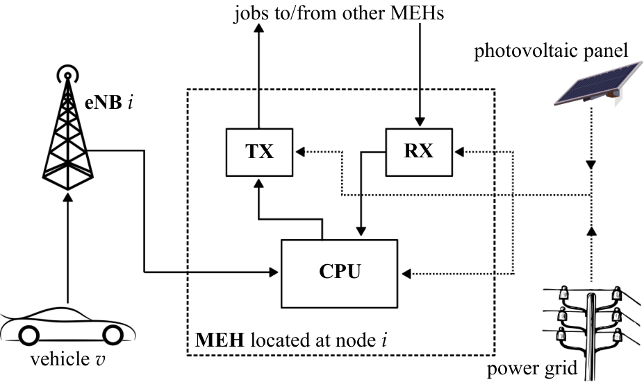
The diagram of an eNB/MEH node is shown in Fig. 2, while a high level diagram of EASE is presented in Fig. 1. The scheduler operates according to two optimization phases:

1. a local phase (left of the diagram): a predictive control phase, performed locally at each MEH node, and 2. a distributed phase (right): a collaborative optimization based on distributed consensus (solved via message passing).

In phase 1, the MEH locally control the ongoing computations, estimating the local processing capacity and energy availability within a given prediction horizon. At the same time, the local algorithm assesses the amount of workload that should be migrated (“desired workload migration estimation”) to the neighboring MEH nodes, predicts the availability of local resources (“MEH resource estimation”), and accounts for mobility estimates (“next MEH prediction”), i.e., the vehicle that generated the job request is about to hand over to a neighboring radio cell.

With phase 2, taking the desired workload to be migrated from phase 1 as input (“neighbors’ resource information”), the MEH collectively reach an agreement (“workload migration agreement”) about how many and which jobs are to be actually migrated, as well as about the target MEH for their migration (“job selection and migration”).

After phase 2), each node updates its local state equations with the new jobs generated by the vehicles under coverage and those received from the neighbors, and goes back to phase 1).

In the remainder, the system model is presented in Section IV. The problem formulation for the optimal scheduling is detailed in Section V. The final scheduling solution, composed of the two phases (local and distributed) is presented in Section VI. The performance assessment is reported in Section VII and final remarks are provided in Section VIII.

Next, we detail the mathematical models for computing and communication services, along with the statistical processes involved in the envisioned scenario and the system constraints. Time $t$ is discrete and evolves according to slots of fixed duration $\tau$ , i.e., $t=0,\tau,2\tau,\dots$ . The mathematical notation is summarized in Table II.

Symbol	Meaning	Unit
$v\in\mathcal{V}$	vehicle ID (ID) and set of vehicles	-
$i\in\mathcal{N}$	eNB/MEH ID and set of eNB/MEH	-
$\mathcal{N}_{i}$ and $N_{i}$	set of neighboring nodes of node $i$ and its cardinality $\|\mathcal{N}_{i}\|$	-
$k\in\mathcal{K}_{i}(t)$ and $K_{i}(t)$	job ID, set of jobs in execution at MEH $i$ at slot $t$ ,	-
$k\in\mathcal{K}_{i}(t)$ and $K_{i}(t)$	and its cardinality $\|\mathcal{K}_{i}(t)\|$	-
$\hat{\mathcal{K}}_{ij}$ and $\hat{K}_{ij}$	set of jobs running on MEH $i$ with probable next MEH $j$	-
$\hat{\mathcal{K}}_{ij}$ and $\hat{K}_{ij}$	and its cardinality	-
$T$	no. of slots in the prediction horizon	-
$t=[0,\ldots,T]$	scheduling time slot index	-
$\tau$	length of a scheduling slot	s
$V_{i}(t)$ and $C_{i}(t)$	no. of results to be sent in the coverage area of eNB $i$ at	-
$V_{i}(t)$ and $C_{i}(t)$	slot $t$ and to be routed through the backhaul network	-
$I_{k}$	intensity of job $k$	cyc.
$D_{k}$	deadline of job $k$	s
$S_{k}$	size of job $k$	bit
$p_{v}$ and $p_{\ell}$	job generation probability and probability that it is of type $\ell$	-
$\bm{p}_{i,k}(t)$	handover prob vector for vehicle $v$ (job $k$ ) at slot $t$
$w_{i,k}(t)$	workload of job $k$ processed by MEH $i$ in slot $t$	cyc.
$L$	(fixed) size of a container instantiated on a MEH	bit
$E_{b}^{\rm RAN}$	energy per bit for eNB-vehicle wireless transmissions	J/bit
$E_{b}^{\rm wired}$	energy per bit for eNB-eNB wired transmission	J/bit
$\sigma_{s}$ and $\sigma_{d}$	energy per bit for migration at the source (destination) MEH	J/bit
$E_{s}$ and $E_{d}$	(fixed) energy for migration at the source (destination) MEH	J
$E^{\rm H}_{i}(t)$	harvested energy available at slot $t$	J
$P_{i}^{\rm PV}(t)$	power supplied by the PV at node $i$ , instant $t$	W
$P_{\rm RAN}$ and $P_{\rm wired}$	(fixed) power to keep the wireless (wired) unit switched on	W
$P_{i}^{\rm idle}$	(fixed) power to keep the server switched on	W
$N_{i}^{\rm inc}(t)$ and $N_{i}^{\rm out}(t)$	no. of MEH incoming (outgoing) jobs at slot $t$	-
$F_{i}$	maximum computational power of server $i$	W
$M_{i}$	maximum amount of RAM available at server $i$	bit
$\bar{w}_{ij}$	desired intensity requested by MEH $i$ to neighbor $j$	cyc./s
$\bar{m}_{ji}$	memory space requested by MEH $i$ to neighbor $j$	bit
$\hat{P}^{\rm H}_{i}$	residual green power at node $i$ after the local scheduling	W
$\hat{F}_{i}$	residual computing power at node $i$ after local scheduling	W
$\hat{M}_{i}$	residual RAM memory at node $i$ after the local scheduling	bit
$o_{ij}$	optimal amount of MEH $i$ processing load to offload to $j$	cyc./s
$\tilde{o}_{ji}$	optimal processing load to be received at MEH $i$ from $j$	cyc./s

TABLE II: Summary of the symbols used within the paper. “cyc.” stands for “CPU cycles”.

Computing job parameters. At time $t$ , each job $k$ served by MEH $i$ is characterized by the triplet $(I_{i,k}(t),D_{i,k}(t),S_{i,k}(t))$ , where

I_{i,k}(t)

is the residual job intensity, expressed in CPU cycles, ii)

D_{i,k}(t)

is the residual (hard) execution deadline, in seconds, i.e., the time still available to execute the job, and iii)

S_{i,k}(t)

is the remaining data to be processed, in bits.

As the job is processed by the server, the intensity, deadline, and data size decrease according to

$\displaystyle I_{i,k}(t+\tau)$	$\displaystyle=I_{i,k}(t)-w_{i,k}(t)\,,$	(1)
$\displaystyle D_{i,k}(t+\tau)$	$\displaystyle=D_{i,k}(t)-\tau\,,$	(2)
$\displaystyle S_{i,k}(t+\tau)$	$\displaystyle=S_{i,k}(t)-\frac{S_{i,k}(0)}{I_{i,k}(0)}w_{i,k}(t)\,,$	(3)

where $w_{i,k}(t)$ is the amount of workload (CPU cycles) belonging to job $k$ and processed by MEH $i$ in slot $t$ , $S_{i,k}(0)$ represents the initial job size (bits), whereas $I_{i,k}(0)$ is the total number of CPU cycles required to fully process the job. Eq. (3) means that the amount of data that is still to be processed decreases linearly with the amount of workload allotted to a job, irrespective of how the workload is distributed in time. Note that (1) makes it possible to rewrite (3) as

\displaystyle S_{i,k}(t)

\displaystyle=\frac{S_{i,k}(0)}{I_{i,k}(0)}I_{i,k}(t).

(4)

Communication models. For the 5G wireless links between the eNB and the vehicles we adopt

i) the massive-MIMO energy consumption model of [29], and ii) the mm-wave –

28

GHz – urban NLoS channel model of [30].

Specifically, from [29] the following system parameters are obtained:

i) the power needed to keep the wireless unit switched on (fixed circuit power consumption),

P_{\textrm{RAN}}

, ii) the energy required per transmitted bit via wireless links,

E_{b}^{\rm RAN}

, iii) the fixed wired circuit power consumption,

P_{\textrm{wired}}

, iv) the energy expenditure for the wired backhaul links connecting the eNB,

E_{b}^{\rm wired}

Note that the vehicles’ energy utilization is not involved in the scheduling and, in turn, only the energy consumption at the eNB side is considered. The model in [30] is used for the vehicle-eNB association.

Container migration model. The migration of a container requires the hosting MEH to spend energy to freeze the status of the virtual entity and prepare the data to be sent to the target MEH for the correct re-instantiation. Hence, the target MEH has to spend energy to create the new virtual entity using the received information. The energy expenditure on the two sides consists of [31]:

i) a contribution proportional to the size of the migration data, through the parameters

\sigma_{s}

and

\sigma_{d}

respectively, plus ii) a fixed energy contribution, equal to

E_{s}

for the source MEH and

E_{d}

for the target one, respectively.

Additionally, the source spends some energy to transmit the data over the wired channel $E_{b}^{\rm wired}$ . Overall, it holds

	$\displaystyle E^{\textrm{migr}}_{\textrm{source}}(t)$	$\displaystyle=\sigma_{s}L+E_{b}^{\rm wired}S_{k}(t)+E_{s},\quad\text{and}$		(5)
	$\displaystyle E^{\textrm{migr}}_{\textrm{dest}}(t)$	$\displaystyle=\sigma_{d}L+E_{d},$		(6)

where $S_{k}(t)$ is the (variable) data size associated with job $k$ , and $L$ is the (fixed) container size. According to [21], we account for a service downtime of $T_{k}^{\rm migr}$ when migrating the entities. In turn, $T_{k}^{\rm migr}$ seconds are additionally removed from the job’s deadline $D_{k}(t)$ at every migration occurrence. Note that the delay associated with wired transmissions is negligible as compared to the service downtime.

Energy harvesting model. We refer to $P_{i}^{\rm PV}(t)$ as the power supplied by the PV co-located with eNB/MEH $i$ at instant $t$ and that varies from a minimum of $P^{\rm PV}_{\rm min}$ to a maximum of $P^{\rm PV}_{\rm max}$ . Accounting for the power required to keep the server ( $P_{i}^{\rm idle}$ ) and the communication channels ( $P_{\rm RAN}$ and $P_{\rm wired}$ ) switched on, and the fixed amount of energy required for the container migration, the harvested energy available at eNB/MEH $i$ for computations and data transmissions at time slot $t$ is

$\displaystyle E^{\rm H}_{i}(t)=$	$\displaystyle\left(P_{i}^{\rm PV}(t)-P_{\rm RAN}-P_{\rm wired}-P_{i}^{\rm idle}\right)\tau\,+$	(7)
	$\displaystyle-N_{i}^{\rm inc}(t)\left(\sigma_{d}\,L+E_{d}\right)\,+$
	$\displaystyle-N_{i}^{\rm out}(t)\left[\left(\sigma_{s}+E_{b}^{\rm wired}\right)L+E_{s}\right]$

where $N_{i}^{\rm inc}(t)$ and $N_{i}^{\rm out}(t)$ are the known number of MEH incoming and outgoing jobs at MEH $i$ and time $t$ , which are scheduled at the previous step $t-\tau$ . The terms in Eqs. (5)-(6) that depend on the data size $S_{i,k}(t)$ are not considered in $E^{\rm H}_{i}(t)$ as they will be integrated in the optimization function (see Eq. (17)). Note that being $E^{\rm H}_{i}(t)$ a difference between the harvested energy and that required to deliver the services, its value can be negative. $E^{\rm H}_{i}(t)$ is known for the current slot $t$ only. However, the developed MPC framework also needs estimates for $[E_{i}^{H}(t+\tau),\ldots,E_{i}^{H}(t+\tau(T-1))]$ , within the time window $t+\tau,\dots,t+\tau(T-1)$ , where $T$ is the prediction horizon. These estimates are computed by forecasting the time-dependent quantities in (7): future values of $P_{i}^{\rm PV}(t+\cdot)$ are estimated using a Gaussian r.v. with average $P_{\rm PV}$ and standard deviation $\sigma_{\rm PV}$ , estimates for the number of incoming $N_{i}^{\rm inc}(t+\cdot)$ and outgoing $N_{i}^{\rm out}(t+\cdot)$ jobs at eNB $i$ in slot $t$ are obtained considering the vehicles in the external annulus of the eNB’s coverage area. Finally, $P_{i}^{\rm idle}$ depends on the specific MEH characteristics at eNB $i$ , as specified in Section VII.

Jobs types and arrival model. Three job types are considered for the numerical results of Section VII, having different intensities, deadlines, and data sizes and identified through the index $\ell=\{1,2,3\}$ . Every job type is associated with a generation triplet $(I^{\ell},D^{\ell},S^{\ell})$ , and a generation probability $p_{\ell}$ . Each vehicle $v\in\mathcal{V}$ can submit at most one computing job at a time to the network facilities, so that a bijective mapping vehicle-job ID can be derived. Once a job is finished or expired, the vehicle submits a new job to the MEH with probability $p_{v}$ at each slot. This parameter is tuned in the simulations. Also in this case, for predictive optimization, an estimate for the future incoming jobs is needed. For this purpose, a circular buffer containing the values of $I_{i,k}/D_{i,k}$ of the newly generated jobs is kept. A fixed estimate of the average of the last $W$ seconds is used to predict the incoming traffic. In [27], the authors verified that even simple predictors are still effective with MPC if $T$ is large enough.

Handover probabilities. Each job $k$ is associated with a probability vector that depends on the position of the vehicle $v$ requesting the service. Being $i$ the serving eNB for vehicle $v$ , we define $\bm{p}_{i,k}(t)$ as the $N_{i}$ -dimensional vector containing the probabilities that vehicle $v$ will hand over to any of the $|\mathcal{N}_{i}|=N_{i}$ neighboring radio cells, i.e., $\bm{p}_{i,k}(t)=[p_{i1,k}(t),p_{i1,k}(t),\dots,p_{iN_{i},k}(t)]$ , with $\sum_{j}p_{ij,k}=1$ . Vector $\bm{p}_{i,k}(t)$ is updated every time a new trajectory sample is available for the associated vehicle $v$ , either inside the same cell or in a new cell after performing the handover.

The set $\mathcal{K}_{i}(t)$ , with cardinality $K_{i}(t)=|\mathcal{K}_{i}(t)|$ , collects the jobs being executed at time slot $t$ at MEH $i$ . The following systems constraints apply
Processing capacity. Indicating with $F_{i}$ the maximum computing power of server $i$ – expressed in CPU cycles per second – the following inequality on the sum of the workloads holds

\frac{1}{\tau}\sum_{k=1}^{K_{i}(t)}w_{i,k}(t)\leq F_{i}\,.

(8)

Storage capacity. Being $M_{i}$ [bits] the maximum amount of RAM available at server $i$ , the sum of the data sizes $S_{i,k}(t)$ of all the active jobs at MEH $i$ must obey

\sum_{k=1}^{K_{i}(t)}S_{i,k}(t)\leq M_{i}\,.

(9)

Job execution time. In case the deadline of job $k$ , $D_{i,k}(t)$ , expires in the current time slot $t$ , the job must be processed entirely and immediately at server $i$ and cannot be further migrated, i.e.,

w_{i,k}(t)=I_{i,k}(t)\qquad\text{if}\;D_{i,k}(t)\leq\tau\,.

(10)

This guarantees the timely delivery of the computation result to the requesting vehicle, avoiding that the outcome becomes useless. As Eqs. (8)-(10) may not be jointly satisfied, in the following we will relax Eq. (8).

Workload conservation. Finally, note that, in general, the inequalities

0\leq w_{i,k}(t)\leq I_{i,k}(t),\;\forall\;i\in\mathcal{N},\;\forall\;k\in\mathcal{K}_{i}(t),\;\forall\;t

(11)

must always hold, because of the workload conservation principle.

Here we formulate the optimization problems concerning the 1) local and 2) distributed scheduling phases introduced in Section III. As shown in Fig. 1, the local and distributed schedulings are run in parallel as distinct tasks that exchange information.

Each MEH $i\in\mathcal{N}$ estimates $w_{i,k}(t)$ for every job $k\in\mathcal{K}_{i}(t)$ to be executed at time $t$ : in the analysis, $w_{i,k}(t)$ stands for the optimal fraction of computing intensity $I_{i,k}(t)$ to be locally executed at time slot $t$ for the hosted job $k$ . We define vectors $\bm{w}_{i}(t)$ , $\bm{I}_{i}(t)$ and $\bm{D}_{i}(t)$ respectively collecting $w_{i,k}(t)$ , $I_{i,k}(t)$ and $D_{i,k}(t)$ for all $k\in\mathcal{K}_{i}(t)$ . As for the energy spent to transmit the processing results back to the vehicles, $V_{i}(t)\,E_{b}^{\rm RAN}$ is the (per bit) energy cost of sending the results to the $V_{i}(t)$ vehicles in the wireless coverage area, while $C_{i}(t)\,E_{b}^{\rm wired}$ is the energy cost entailed in routing the $C_{i}(t)$ jobs that are completed at node $i$ and that have to be routed via the backhaul links to reach the corresponding user (vehicle). $R_{k}$ is the size of the processing result of job $k$ , and $q_{i}^{\rm proc}$ is the energy cost of processing a unit of workload.

Given these quantities, we define two local (at node $i$ ) functions $f_{i}(\cdot)$ and $g_{i}(\cdot)$ , as follows.

	$\displaystyle f_{i}(\bm{w}_{i};V_{i},C_{i},E^{\rm H}_{i})=$	$\displaystyle q_{i}^{\rm proc}\bm{1}^{\scriptscriptstyle{T}}\bm{w}_{i}(t)+V_{i}(t)\,E_{b}^{\rm RAN}R_{k}\,+$		(12)
		$\displaystyle+C_{i}(t)\,E_{b}^{\rm wired}R_{k}-E^{\rm H}_{i}(t)\,,$		(12)

g_{i}(\bm{I}_{i}(t);\bm{D}_{i}(t))=\sum_{k=1}^{K_{i}(t)}\left(\frac{I_{i,k}(t)}{D_{i,k}(t)}\right)^{2}.

(13)

$f_{i}(\cdot)$ quantifies the difference between the total energy expenditure at node $i$ in slot $t$ (due to processing and communications processes) and the energy that is locally harvested at this node. Hence, $-f(\bm{w}_{i};\cdot)$ represents the residual cost-free energy available for the migration process in the distributed phase. Minimizing $f_{i}(\cdot)$ corresponds to maximizing the local energy available at the node. $g_{i}(\cdot)$ represents the residual processing cost, which is proportional to $(I_{i,k}/D_{i,k})^{2}$ . Minimizing $g_{i}(\cdot)$ forces the node to execute the jobs, especially prioritizing those with high intensity and whose deadline is about to expire. Note also that, due to Eq. (1), $I_{i,k}(t)$ depends on the optimization variable $w_{i,k}$ at previous time slots.

Considering a forecast optimization window of $T$ slots into the future, and letting $t=0$ be the current time slot, the local cost function at node $i$ over the whole time horizon is formulated by combining $f_{i}(\cdot)$ and $g_{i}(\cdot)$ , as

	$\displaystyle J_{i}\left(\mathcal{W}_{i},\mathcal{I}_{i};\mathcal{D}_{i},\bm{V}_{i},\bm{C}_{i},\bm{E}^{\rm H}_{i}\right)=$	$\displaystyle\gamma\sum_{t=0}^{T-1}\,g_{i}(\bm{I}_{i}(t);\bm{D}_{i}(t))\,+$		(14)
		$\displaystyle+\sum_{t=0}^{T-1}\max\{f_{i}(\bm{w}_{i};\cdot),0\}^{2},$		(14)

where $\mathcal{W}_{i}$ , $\mathcal{I}_{i}$ and $\mathcal{D}_{i}$ represent the stacks of vectors $\bm{w}_{i}(t)$ , $\bm{I}_{i}(t)$ and $\bm{D}_{i}(t)$ over the considered horizon $T$ , respectively, while $\bm{V}_{i}$ , $\bm{C}_{i}$ and $\bm{E}^{\rm H}_{i}$ are the vectors collecting $V_{i}(t)$ , $C_{i}(t)$ and $E^{\rm H}_{i}(t)$ for $t\in\{0,\tau,\dots,\tau(T-1)\}$ . The coefficient $\gamma>0$ is used to balance the processing state cost term ( $g_{i}(\cdot)$ ) with respect to the energy cost ( $f_{i}(\cdot)$ ).

From a physical perspective, the processing energy consumption is not necessarily a quadratic function, but it varies based on the specific computing architecture [32]. A quadratic function for $f_{i}(\cdot)$ was chosen, as it promotes smoothness of the controller in the transitions from one slot to the next one, and has the same curvature order of the processing state cost $g_{i}(\cdot)$ . Also, the $\max\{\cdot\}$ function is used to make the cost positive only when $f_{i}(\cdot)>0$ , i.e., the renewable energy is fully used and the node has to resort to the power grid.

Next, the cost function in Eq. (14) is modified through the addition of a penalty term proportional to two non-negative auxiliary variables $\bm{\delta}_{i}(t)=[\delta_{F_{i}}(t),\delta_{M_{i}}(t)]$ , to ensure that the problem does not become infeasible when resources are scarce. Therefore, rewriting the constraints (8) and (9), we define for each MEH the following local problem at node $i$ ,

where $\bm{c}_{i}=[c_{F_{i}},c_{M_{i}}]$ is the vector collecting the coefficients weighting the penalty variables, with $c_{F_{i}},c_{M_{i}}>0$ . By solving (15), each MEH obtains the optimal control $\bm{w}_{i}(0)$ which is implemented in the current time step.

From (15), each server estimates its future energy and processing resources. Specifically, let $\hat{P}^{\rm H}_{i}$ be the residual available green power, possibly negative if the grid support is sought, $\hat{F}_{i}$ , and $\hat{M}_{i}$ be the residual computational power, and RAM memory at node $i$ , respectively. Note that, since constraints (8) and (9) are relaxed in (15), $\hat{F}_{i}$ and $\hat{M}_{i}$ can be negative. These estimates are obtained by averaging the values over the prediction horizon, excluding the current instant $t=0$ . Due to this averaging operation, while in (15) we deal with energy expenditures, in the following we refer to power quantities.

The migration task presents itself as a combinatorial MIP (MIP) problem, which is non-convex and is generally difficult to solve in a distributed fashion. Thus, we use heuristics to derive approximated solutions. In this work, the popular relax and round method is used, which consists in solving the convex counterpart of the original problem, and rounding the result to a feasible solution afterward. The reason for this choice is that it allows tackling the problem in a distributed fashion via message passing, solving the continuous form problem exactly to the optimum. Other approaches would have required a centralized solution or the design of a heuristic inspired by the optimization objective.

Based on the handover probability vector $\bm{p}_{i,k}$ presented in Section IV-B, each MEH determines the average resource demand requested from its neighbors in the migration process. Specifically, the CPU cycles per second and memory space that are requested from neighbor $j$ are

\bar{w}_{ij}=\sum_{k\in\hat{\mathcal{K}}_{ij}}\frac{I_{i,k}}{D_{i,k}}\,,\,\,\,\text{and}\,\,\,\bar{m}_{ij}=\sum_{k\in\hat{\mathcal{K}}_{ij}}S_{i,k}\,,

(16)

respectively, where $\hat{\mathcal{K}}_{ij}$ contains the set of jobs that are currently running at server $i$ , associated with vehicles that are about to leave the coverage area of the co-located eNB $i$ and whose most probable next eNB is co-located with MEH $j$ . With $\bar{\bm{w}}_{i}=[\bar{w}_{i1},\ldots,\bar{w}_{iN_{i}}]$ we denote the vector collecting the desired processing intensity per second to be sent to each of the $N_{i}$ neighbors of MEH $i$ , computed via (16). We also introduce the new optimization variables $\bm{o}_{i}=[o_{i1},\ldots,o_{iN_{i}}]$ and $\tilde{\bm{o}}_{i}=[\tilde{o}_{1i},\ldots,\tilde{o}_{N_{i}i}]$ representing the optimal total amount of processing load to be sent to, and to be received from each neighbor, respectively. The deviation from the desired $\bar{\bm{w}}_{i}$ to be migrated is penalized with the $l_{2}$ -norm $\|\bar{\bm{w}}_{i}-\bm{o}_{i}\|^{2}$ , and the migration cost is defined as

$\displaystyle\Gamma_{i}\left(\bm{o}_{i},\tilde{\bm{o}}_{i};\bar{\bm{w}}_{i},\hat{P}^{\rm H}_{i}\right)=$	$\displaystyle\max\big\{\left(q_{i}^{\rm tx}-q_{i}^{\rm proc}\right)\bm{1}^{\scriptscriptstyle{T}}\bm{o}_{i}\,+$	(17)
	$\displaystyle+\left(q_{i}^{\rm rx}+q_{i}^{\rm proc}\right)\bm{1}^{\scriptscriptstyle{T}}\tilde{\bm{o}}_{i}-\hat{P}^{\rm H}_{i},0\big\}\,+$
	$\displaystyle+\rho\\|\bm{o}_{i}-\bar{\bm{w}}_{i}\\|^{2}\,,$

where $q_{i}^{\rm proc}$ , $q_{i}^{\rm tx}$ and $q_{i}^{\rm rx}$ are the processing, transmission and reception costs of server $i$ (expressed as powers), respectively. The $\max\{\cdot\}$ term accounts for the power that would be drained from the power grid to migrate the jobs, whereas the quadratic term encodes the fact that the optimal $\bm{o}_{i}$ should be as close as possible to the desired $\bar{\bm{w}}_{i}$ – this corresponds to moving the jobs to the next serving eNB. Finally, $\rho>0$ is a weight balancing the importance of the two cost terms. Note that minimizing Eq. (17) returns a solution $\bm{o}_{i}$ that matches vector $\bar{\bm{w}}_{i}$ if the residual harvested power is sufficient and the constraints are satisfied. Specifically, as system constraint we consider the following variation of (8) and (9), introducing a variable $\hat{\delta}_{i}\geq 0$ , as follows,

\sum_{j\in\mathcal{N}_{i}}\left(\tilde{o}_{ji}-o_{ij}\right)\leq\min\{\hat{F}_{i},\xi_{M_{i}}\hat{M}_{i}\}+\hat{\delta}_{i},\qquad\forall\,i\in\mathcal{N}.

(18)

The meaning of (18) is that the workload surplus that server $i$ has during the following time steps, i.e., the incoming workload minus the outgoing one, should satisfy the average (long-term) power ( $\hat{F}_{i}$ ) and memory ( $\hat{M}_{i}$ ) availability at node $i$ . The coefficient $\xi_{M_{i}}$ relates the memory availability to the residual computational power. This follows from the assumption of direct proportionality between the data size $S_{k}$ and the processed workload $w_{k}$ .

Since the general goal is to minimize the energy drained network-wide from the power grid, a cost function that represents the global welfare and at that at the same time is amenable to a distributed solution is the sum

\Gamma\left(\bm{o},\tilde{\bm{o}},\hat{\bm{\delta}};\bar{\bm{w}},\hat{\bm{P}}^{\rm H}\right)=\sum_{i\in\mathcal{N}}\left[\Gamma_{i}\left(\bm{o}_{i},\tilde{\bm{o}}_{i};\bar{\bm{w}}_{i},\hat{P}^{\rm H}_{i}\right)+\hat{c}_{i}\hat{\delta}^{2}_{i}\right],

(19)

where $\hat{c}_{i}>0$ is the cost coefficient associated with the penalty term $\hat{\delta}_{i}^{2}$ . This leads to the constrained optimization problem

$\displaystyle P^{\rm glob}:$		$\displaystyle\min_{\bm{o},\tilde{\bm{o}},\hat{\bm{\delta}}}$	$\displaystyle\Gamma\left(\bm{o},\tilde{\bm{o}},\hat{\bm{\delta}};\bar{\bm{w}},\hat{\bm{P}}^{\rm H}\right)$	(20)
$\displaystyle\text{s.t.}$	$\displaystyle\bm{o},\tilde{\bm{o}},\hat{\bm{\delta}}\geq 0,\;\eqref{eq:distr_proc_constraint},$
	$\displaystyle o_{ij}=\tilde{o}_{ij}\;\forall\,i,j,$

with $\bm{o}$ , $\tilde{\bm{o}}$ , $\hat{\bm{\delta}}$ , $\bar{\bm{w}}$ and $\hat{\bm{P}}^{\rm H}$ are vectors collecting $\bm{o}_{i}$ , $\tilde{\bm{o}}_{i}$ , $\hat{\delta}_{i}$ , $\bar{\bm{w}}_{i}$ and $\hat{P}_{i}^{{\rm H}}$ respectively, for all the MEH $i\in\mathcal{N}$ . The equality $o_{ij}=\tilde{o}_{ij}$ is called consensus constraint and ensures that the amount of workload exiting node $i$ and directed to $j$ equals the one that $j$ expects to receive from $i$ .

The local problem (15) is used to schedule the amount of workload $w_{i}$ (CPU cycles) that is to be executed locally at each MEH in the current time slot $t$ . Since the solution is predictive, it uses future memory availability ( $\hat{M}_{i}$ ) and residual computational power ( $\hat{F}_{i}$ ) estimates to set the global problem constraints (18). Thanks to the global problem (20) an agreement is reached on which jobs are to be migrated and where. The solution ${\bm{o}}_{i}$ of the global problem is utilized to move workload across the MEHs: this entails an update of sets $\mathcal{K}_{i}(t+1)$ containing the jobs that are assigned to MEH $i$ at the next time slot $t+1$ . The optimization keeps iterating between local and distributed phases.

At each MEH, the local MPC problem of (15) is solved over the whole horizon $T$ [33]. MPC uses the receding horizon technique, which consists of solving the given problem within a prediction window of size $T$ , applying the optimal computed control only for the current time step $t=0$ , moving forward the optimization window by one time slot ( $\tau$ seconds) and repeating the procedure. In this way, the controller progressively adapts to new observations and estimates of the exogenous processes. Also, at any given instant, MEH $i$ computes the optimal policy throughout the whole horizon of $T$ slots, but only $\bm{w}_{i}(0)$ is applied as the control action. The exogenous processes are the future jobs and the harvested energy availability, see Section IV-B.

In the following, the scheduling slot index $t$ is omitted in the interest of readability. Eq. (20) is a consensus problem, i.e., it entails reaching an agreement on the value of some variables among multiple agents in a distributed system. In our context, the MEH must agree on the amount of processing load to exchange among each other. A way to solve this problem – written as the sum of separable convex cost functions – is via the dual ascent algorithm [34]. Given a generic cost function $\psi(\bm{x})$ , its Lagrangian is defined as

\mathcal{L}(\bm{x},\bm{z})=\psi(\bm{x})+\bm{z}^{T}(A\bm{x}-\bm{d})\,,

(21)

where $\bm{z}$ are the Lagrange multipliers associated with the constraints $A\bm{x}=\bm{d}$ . The dual ascent solves the problem by iteratively

i) minimizing

\mathcal{L}(\bm{x},\bm{z})

with respect to

\bm{x}

(primal step), and ii) updating the value of

\bm{z}

(dual step).

To formalize the solution of problem (20) via dual ascent, we split the local cost functions (17) as

$\displaystyle\tilde{\Gamma}_{i}\left(\bm{o}_{i},\tilde{\bm{o}}_{i},\hat{\delta}\right)=$	$\displaystyle\max\big\{\left(q_{i}^{\rm tx}-q_{i}^{\rm proc}\right)\bm{1}^{\scriptscriptstyle{T}}\bm{o}_{i}\,+$	(22)
	$\displaystyle+\left(q_{i}^{\rm rx}+q_{i}^{\rm proc}\right)\bm{1}^{\scriptscriptstyle{T}}\tilde{\bm{o}}_{i}-\hat{P}^{\rm H}_{i},0\big\}\,+$
	$\displaystyle+\frac{\rho}{2}\\|\bm{o}_{i}-\bar{\bm{w}}_{i}\\|^{2}+\frac{\rho}{2}\\|\tilde{\bm{o}}_{i}-\tilde{\bm{w}}_{i}\\|^{2}+\hat{c}_{i}\hat{\delta}_{i}^{2},$

exploiting the fact that $o_{ij}=\tilde{o}_{ij}$ , and defining $\tilde{\bm{w}}_{i}=\{\bar{w}_{ji}\,|\,j\in\mathcal{N}_{i}\}$ . Intuitively, node $i$ is responsible for half of the quadratic cost from its neighbors and for half of its own local cost. For compactness, let $\bm{x}=\{\bm{x}_{i}=[\bm{o}_{i},\tilde{\bm{o}}_{i},\hat{\delta}_{i}],\,\forall\,i\in\mathcal{N}\}$ be the global optimization variable, $\bm{b}_{i}=[\bar{\bm{w}}_{i},\tilde{\bm{w}}_{i},0]$ the tracking target vector, and $\bm{q}_{i}=[\bm{q}^{\textrm{tx}}_{i}-\bm{q}^{\textrm{proc}}_{i},\bm{q}^{\textrm{rx}}_{i}+\bm{q}^{\textrm{proc}}_{i},0]$ the linear costs vector. Moreover, we define matrix $Q_{i}=I_{2N_{i}+1}\bm{m}_{i}$ , with $\bm{m}_{i}=[\frac{\rho}{2},\ldots\frac{\rho}{2},\hat{c}_{i}]$ , and the global block diagonal matrix $Q$ , collecting each $Q_{i}$ on the diagonal. With these definitions, problem (20) can be expressed in the following form

$\displaystyle\min_{\bm{x}}\quad$	$\displaystyle\sum_{i\in\mathcal{N}}\Big(\\|\bm{x}_{i}-\bm{b}_{i}\\|^{2}_{Q_{i}}+\max\left\{\bm{q}_{i}^{T}\bm{x}_{i}-\hat{P}^{\rm H}_{i},0\right\}\Big)$	(23)
s.t.	$\displaystyle A_{1}\,\bm{x}\leq\bm{d},$	(24)
	$\displaystyle A_{2}\,\bm{x}=\bm{0},$	(25)

where $\|\bm{x}\|^{2}_{Q}=\bm{x}^{\scriptscriptstyle{T}}Q\bm{x}$ . The inequalities (24) collect (18) and the non-negativity constraints $\bm{o},\tilde{\bm{o}},\hat{\bm{\delta}}\geq 0$ , while the equalities (25) correspond to the consensus constraints $o_{ij}=\tilde{o}_{ij}$ , $\forall i\in\mathcal{N}$ , $j\in\mathcal{N}_{i}$ . Here, matrices $A_{1}$ and $A_{2}$ are used to select the concerned variables, whereas $\bm{d}=\{\bm{d}_{i}=[\min\{\hat{F}_{i},\xi_{M_{i}}\hat{M}_{i}\},\bm{0}]\mid i\in\mathcal{N}\}$ . We can now write the Lagrangian as

\mathcal{L}\left(\bm{x},\bm{y},\bm{z}\right)=\sum_{i\in\mathcal{N}}\tilde{\Gamma}_{i}\left(\bm{x}_{i};\bm{b}_{i},\hat{P}^{\rm H}_{i}\right)+\bm{y}^{T}\left(A_{1}\bm{x}-\bm{d}\right)+\bm{z}^{T}A_{2}\bm{x}\,,

(26)

where $\bm{y}=\{\bm{y}_{i}=[\lambda_{i},\bm{\gamma}_{i},\tilde{\bm{\gamma}}_{i},\hat{\varphi}_{i}]\,|\,i\in\mathcal{N}\}$ are the Lagrange multipliers associated with the inequality constraints (24), and $\bm{z}=\{\bm{z}_{i}=\bm{\mu}_{i}\,|\,i\in\mathcal{N}\}$ are the multipliers associated with equalities (25). Specifically, the Lagrange multipliers $\lambda_{i}$ refer to constraints (18), $\bm{\gamma}_{i}=\{\gamma_{ij}\}$ , $\tilde{\bm{\gamma}}_{i}=\{\tilde{\gamma}_{ji}\}$ and $\hat{\varphi}_{i}$ to $\bm{o}_{i}\geq 0$ , $\tilde{\bm{o}}_{i}\geq 0$ , and $\hat{\delta}_{i}\geq 0$ , respectively, and $\bm{\mu}_{i}=\{\mu_{ij}\}$ to $o_{ij}=\tilde{o}_{ij}$ , for every server $i\in\mathcal{N}$ , and $j\in\mathcal{N}_{i}$ . Using the ⁺ sign to denote the update at the following iteration, we detail in Algorithm 1 the dual ascent procedure that solves the problem

\inf_{\bm{x}}\;\sup_{\bm{y}\geq 0,\bm{z}}\;\mathcal{L}\left(\bm{x},\bm{y},\bm{z}\right).

(27)

Algorithm 1 Dual ascent algorithm solving problem (20)

\bm{x}^{+}=\argmin_{\bm{x}}\;\mathcal{L}\left(\bm{x};\bm{y},\bm{z}\right)

\triangleright

primal

\bm{y}^{+}=\max\left\{\bm{y}+\bm{\alpha}_{\bm{y}}\left(A_{1}\,\bm{x}^{+}-\bm{d}\right),0\right\}

\triangleright

dual (ineq.)

\bm{z}^{+}=\bm{z}+\bm{\alpha}_{\bm{z}}A_{2}\,\bm{x}^{+}

\triangleright

dual (eq.)

The dual update requires in this case two different forms, depending on whether the constraint is an equality or an inequality one. Inequality constraints may actually be inactive, and the associated Lagrange multipliers would be null in this case. The parameters $\bm{\alpha}_{\bm{y}}$ and $\bm{\alpha}_{\bm{z}}$ in the algorithm tune the stability and the convergence speed. The presented compact version of the dual ascent translates into the following local procedure, from a server perspective. Defining vectors $\tilde{\bm{\mu}}_{i}=\{\mu_{ji}\}$ and $\bar{\bm{o}}_{i}=\{\tilde{o}_{ij}\}$ to collect those variables that are kept in memory by the neighborhoods of $i$ , the local Lagrangian at node $i$ is

$\displaystyle\mathcal{L}_{i}\left(\bm{x}_{i};\bar{\bm{w}}_{i},\tilde{\bm{w}}_{i},\hat{P}^{\rm H}_{i},\bm{\nu}_{i}\right)=$	$\displaystyle\tilde{\Gamma}_{i}\left(\bm{o}_{i},\tilde{\bm{o}}_{i};\bar{\bm{w}}_{i},\tilde{\bm{w}}_{i},\hat{P}^{\rm H}_{i}\right)\,+$	(28)
	$\displaystyle+\lambda_{i}\left[\bm{1}^{T}(\tilde{\bm{o}}_{i}-\bm{o}_{i})-\hat{\delta}_{i}\right]+$
	$\displaystyle-\bm{\gamma}_{i}^{T}\bm{o}_{i}-\tilde{\bm{\gamma}}_{i}^{T}\tilde{\bm{o}}_{i}+\bm{\mu}_{i}^{T}\bm{o}_{i}\,+$
	$\displaystyle-\tilde{\bm{\mu}}_{i}^{T}\tilde{\bm{o}}_{i}-\hat{\varphi}_{i}\hat{\delta}_{i},$

with $\bm{x}_{i}=[\bm{o}_{i}^{+},\tilde{\bm{o}}_{i}^{+},\hat{\delta}_{i}]$ and $\bm{\nu}_{i}=[\lambda_{i}\bm{1},\varphi_{i},\bm{\gamma}_{i},\tilde{\bm{\gamma}}_{i},\bm{\mu}_{i},\tilde{\bm{\mu}}_{i}]$ to collect the Lagrange multipliers. The local procedure is presented in Algorithm 2, where a fixed step size $\alpha$ is assumed.

Algorithm 2 Dual ascent from a server perspective

1: receive

\tilde{\bm{\mu}}_{i}=\{\mu_{ji}\}

from the neighbors

[\bm{o}_{i}^{+},\tilde{\bm{o}}_{i}^{+},\hat{\delta}_{i}]=\argmin_{\bm{x}_{i}}\;\mathcal{L}_{i}\left(\bm{x}_{i};\bar{\bm{w}}_{i},\tilde{\bm{w}}_{i},\hat{P}^{\rm H}_{i},\bm{\nu}_{i}\right)

3: send

\tilde{o}_{ji}^{+}

to the corresponding neighbor

j

\lambda_{i}^{+}=\max\left\{\lambda_{i}+\alpha\left(\sum_{j\in\mathcal{N}_{i}}\left(\tilde{o}_{ji}^{+}-o_{ij}^{+}\right)-\hat{F}_{i}\right),0\right\}

\hat{\varphi}_{i}^{+}=\max\left\{\hat{\varphi}_{i}-\alpha\,\hat{\delta}_{i}^{+},0\right\}

\bm{\gamma}_{i}^{+}=\max\left\{\bm{\gamma}_{i}-\alpha\,\bm{o}_{i}^{+},0\right\}

\tilde{\bm{\gamma}}_{i}^{+}=\max\left\{\tilde{\bm{\gamma}}_{i}-\alpha\,\tilde{\bm{o}}_{i}^{+},0\right\}

8: receive

\bar{\bm{o}}_{i}^{+}=\{\tilde{o}_{ij}^{+}\}

from the neighbors

\bm{\mu}_{i}^{+}=\bm{\mu}_{i}+\alpha\left(\bm{o}_{i}^{+}-\bar{\bm{o}}_{i}^{+}\right)

10: send

\mu_{ij}^{+}

to the corresponding neighbor

j

Note that, to minimize the Lagrangian in the primal step at line 2, server $i$ not only needs its own Lagrange multipliers, but also the introduced $\tilde{\bm{\mu}}_{i}$ , which collects the $\mu_{ji}$ of neighbors $j\in\mathcal{N}_{i}$ . Therefore, node $i$ must first receive these multipliers from the neighborhood. Also, while updating $\bm{\mu}_{i}$ in the dual step at line 9, $\bar{\bm{o}}_{i}^{+}$ is needed, which collects the $\tilde{o}_{ij}^{+}$ variables kept by the neighborhood of $i$ , and which are to be received after the computation of $j$ ’s primal step ( $\forall j\in\mathcal{N}_{i}$ ). Hence, this amounts to two communication rounds among neighbors per dual ascent iteration. The dual updates are computationally inexpensive, whereas the primal step requires solving a local convex subproblem, which is complicated by the $\max\{\cdot\}$ operator in the cost function (22). Eventually, note that an additional communication is required at the beginning of the procedure, to inform the neighborhood about the values of $\tilde{\bm{w}}_{i}$ .

Solution to the primal step (line 2). The solution of the local primal subproblems is computed in closed form, distinguishing three cases. We consider the local primal subproblems in compact form with variables $\bm{x}_{i}$ , and collect the Lagrange multipliers of (28) in $\bm{\nu}_{i}=[\lambda_{i}\bm{1},\varphi_{i},\bm{\gamma}_{i},\tilde{\bm{\gamma}}_{i},\bm{\mu}_{i},\tilde{\bm{\mu}}_{i}]$ , with associated variables selection matrix $A_{i}$ . We split $\mathcal{L}_{i}\left(\bm{x}_{i};\cdot\right)=u_{i}\left(\bm{x}_{i}\right)+h_{i}\left(\bm{x}_{i}\right)$ , so that

	$\displaystyle u_{i}\left(\bm{x}_{i}\right)$	$\displaystyle=\\|\bm{x}_{i}-\bm{b}_{i}\\|^{2}_{Q_{i}}+\bm{\nu}_{i}^{T}A_{i}\bm{x}_{i},$		(29)
	$\displaystyle h_{i}\left(\bm{x}_{i}\right)$	$\displaystyle=\bm{q}_{i}^{T}\bm{x}_{i}-\hat{P}^{\rm H}_{i}.$		(30)

The solution of the primal step of problem (20) is computed as one of the mutually exclusive cases

i)

$\bm{x}_{i}^{+}=\argmin_{\bm{x}_{i}}u_{i}\left(\bm{x}_{i}\right)$ , if $h_{i}\left(\bm{x}_{i}^{+}\right)\leq 0$ , or
ii)

$\bm{x}_{i}^{+}=\argmin_{\bm{x}_{i}}u_{i}\left(\bm{x}_{i}\right)+h_{i}\left(\bm{x}_{i}\right)$ , if $h_{i}\left(\bm{x}_{i}^{+}\right)>0$ , or
iii)

$\bm{x}_{i}^{+}=\argmin_{\bm{x}_{i}}u_{i}\left(\bm{x}_{i}\right)$ , s.t. $h_{i}\left(\bm{x}_{i}\right)=0$ .

The solutions for each of the cases of Proposition 1 are now given in the following result.

Consider the three cases of Proposition 1. Their closed form optimal solutions are expressed as

i)

$\bm{x}_{i}^{+}=\bm{b}_{i}-\frac{1}{2}\,Q_{i}^{-1}A_{i}^{\scriptscriptstyle{T}}\bm{\nu}_{i}$
ii)

$\bm{x}_{i}^{+}=\bm{b}_{i}-\frac{1}{2}\,Q_{i}^{-1}\left(A_{i}^{\scriptscriptstyle{T}}\bm{\nu}_{i}+\bm{q}_{i}\right)$
iii)

$\bm{x}_{i}^{+}=\bm{b}_{i}-\frac{1}{2}\,Q_{i}^{-1}\left(A_{i}^{\scriptscriptstyle{T}}\bm{\nu}_{i}+\bm{q}_{i}^{\scriptscriptstyle{T}}\frac{2\,Q_{i}\left(\bm{b}_{i}-\frac{\hat{P}^{\rm H}_{i}}{\|\bm{q}_{i}\|^{2}}\bm{q}_{i}\right)-A_{i}^{\scriptscriptstyle{T}}\bm{\nu}_{i}}{\|\bm{q}_{i}\|^{2}}\bm{q}_{i}\right)$

The proofs of Propositions 1 and 2 are given in Appendix A, together with the theoretical upper bound for the step size $\alpha$ that guarantees convergence.

In this section, we show how to compute the actual discrete allocation of jobs by obtaining new variables $\bm{o}_{i}^{r}$ , which are the rounded versions of the $\bm{o}_{i}$ that were previously computed through consensus (see Section VI-B). In particular, $\bm{o}_{i}$ contains the optimal continuous amount of workload that each MEH would like to send to its neighbors. Instead, its rounded version $\bm{o}_{i}^{r}$ contains a feasible allocation accounting for the fact that the number of jobs and the possible ways of allocating them are discrete.

To compute the new $\bm{o}_{i}^{r}$ , as an initial solution, we select the jobs from set $\hat{\mathcal{K}}_{ij}$ , whose associated vehicle is about to migrate from eNB site $i$ to $j$ . The rounded $\bm{o}_{i}^{r}$ is thus initially set to $\bar{\bm{w}}_{i}$ , assuming that the minimizer of the objective function (17) is the vector that minimizes the quadratic term. Then, the difference between this guess and the actual optimum obtained from the proposed dual ascent algorithm is computed, $\bm{o}_{i}^{\rm diff}$ . For every neighbor $j$ it is now clear whether more workload is to be added to (in case $o_{ij}^{\rm diff}<0$ ) or removed from ( $o_{ij}^{\rm diff}>0$ ) the initial guess $o_{ij}^{r}$ . The jobs that were initially scheduled for migration to node $j$ but that are eventually retained for computation at node $i$ are those minimizing $\|\bm{o}_{i}^{\rm diff}\|_{{}_{1}}$ . Instead, new jobs are added to the migration list using the prediction vectors $\bm{p}_{ij}$ . In detail, the added jobs are those for which the handover probabilities towards $j$ are maximized. A threshold $\epsilon_{P}$ is used to approximate the rounded solution, as the continuous optimum $\bm{o}_{i}$ will likely not coincide with any possible discrete approximation. The procedure is detailed in Algorithm 3.

Algorithm 3 Job-neighbor association

1: Input: mobility pattern predictions matrix

P_{i}

; optimal outgoing workload amount

\bm{o}_{i}

; set of the jobs

\mathcal{J}_{i}

in execution at MEH

i

; tolerance threshold

\epsilon_{P}

2: Output: job-neighbor association sets

\mathcal{Z}_{ij}\,\forall\,j\in\mathcal{N}_{i}

; rounded

\bm{o}_{i}^{r}

3: remove jobs

\{k\mid I_{i,k}<\epsilon\vee D_{i,k}<2\}

from

\mathcal{J}_{i}

\bm{o}_{i}^{r}\leftarrow\bar{\bm{w}}_{i}

\mathcal{Z}_{ij}\leftarrow\hat{\mathcal{K}}_{ij}

\mathcal{J}_{i}\leftarrow\mathcal{J}_{i}\setminus\bigcup_{j\in\mathcal{N}_{i}}\hat{\mathcal{K}}_{ij}

\bm{o}_{i}^{\rm diff}\leftarrow\bm{o}_{i}^{r}-\bm{o}_{i}

\triangleright

workload to be adjusted

8: for all neighbors

j

\mathcal{N}_{i}

9: while

o_{ij}^{\rm diff}>\epsilon_{P}

10:

k\leftarrow

job of

\mathcal{Z}_{ij}

minimizing

\left|\,o_{ij}^{\rm diff}\right|

11: remove job

k

from

\mathcal{Z}_{ij}

12:

o_{ij}^{r}\leftarrow o_{ij}^{r}-I_{i,k}/D_{i,k}

13:

o_{ij}^{\rm diff}\leftarrow o_{ij}^{\rm diff}-I_{i,k}/D_{i,k}

14: add job

k

\mathcal{J}_{i}

\triangleright

make it available for neighbors

15: end while

16: while

o_{ij}^{\rm diff}<-\epsilon_{P}

17: take

k\in\mathcal{J}_{i}\mid k\in\argmax\bm{p}_{ij}

\triangleright

most prob.

i\rightarrow j

18: add job

k

\mathcal{Z}_{ij}

19:

o_{ij}^{r}\leftarrow o_{ij}^{r}+I_{i,k}/D_{i,k}

20:

o_{ij}^{\rm diff}\leftarrow o_{ij}^{\rm diff}+I_{i,k}/D_{i,k}

21: mask entry

p_{ij,k}

\triangleright

s.t.

k

is not selected again

22: end while

23: end for

Handling pathological cases: Since system constraints are made soft to avoid primal infeasibility, three pathological cases may arise, namely,

1. the optimal processed workload at the current instant exceeds the computational capacity; or 2. the data size for the currently running jobs do not fit the RAM memory; or 3. the deadline expires during the current slot, but the residual intensity is greater than zero.

A greedy algorithm is developed to handle all of them. For the first two, the MEH ranks the active jobs through a double ordering criterion, considering as the first ranking criterion the time slot when they expire, and as the second their intensity (or data size). Next, it momentarily pauses the execution of the services starting from the last one in the ordered list, until the resources suffice to proceed. In case 1, when pausing a job $m$ , the amount of processed workload becomes $\sum_{k\in\mathcal{K}_{i}}w_{i,k}-w_{i,m}$ , while in case 2, the data relative to suspended jobs is deleted from the RAM. The number of suspended jobs is the minimum such that the requirements are satisfied. Moreover, in case 1, it is likely that, when a job is suspended, additional computational power becomes available. In such a case, the new computational resources are assigned to the jobs that are closest to their deadline. Case 3 is managed considering the amount of residual intensity $I_{i,k}$ . If $I_{i,k}$ is smaller than a threshold $\epsilon$ , then the deadline is extended by a small amount, so that the controller will privilege the execution of the corresponding job in the next slot. In this way, jobs are allowed to finish with a little additional delay (within one slot). If, however, the amount of residual intensity is larger than $\epsilon$ , the job is dropped, i.e., in this case the algorithm failed to provide an acceptable solution.

Algorithm complexity: The decomposition approach adopted in EASE makes the overall algorithm feasible and lightweight to be run even in a complex and highly variable scenario such as the vehicular one here considered. Previous work [27] uses MPC to obtain an optimal decision on both the amount of workload to process locally and to offload to other MEH in a fully decentralized fashion. This amounts to having a number of shared variables to be optimized via message passing $\mathcal{O}(VT)$ , where $V$ is the number of edges in the network graph and $T$ is the prediction window. EASE, instead, by performing a preliminary local optimization phase, estimates the future on average, having thus a number of shared variables $\mathcal{O}(V)$ . The local phase amounts to solving a constrained convex problem numerically every $\tau$ seconds, while the distributed phase requires broadcasting to the neighborhood (a part of) the primal and dual information of problem (20), plus inexpensive closed form updates. Note that this information amounts to a few bits only, which can be easily piggybacked on control packets that the MEH normally exchange for other reasons. The empirical convergence rate is studied in Section VII-C.

Predictions inaccuracies: With the adopted approach, a residual migration suboptimality is still possible also due to prediction errors on the mobility of the users, the service request, and the available local resources. Concerning the mobility prediction, the performance is extensively studied in [8], where the authors compare the mobility predictor also used by EASE with a simpler and less accurate approach based on Markov chains, showing the improvement brought by considering the information on the actual trajectory followed by the users. However, we recall that the main objective of EASE is to reduce the carbon footprint and, in turn, even in the case of precise mobility predictions, the scheduler can decide to place the service in a MEH that is far away from the vehicle, it this leads to better use of the energy resources. For this reason, the eNB/MEH are connected via backhaul links that always ensure that the result is sent back to the user. Regarding instead the statistical processes that control the energy availability and the job requests, with EASE we only assume to know the average income over a prediction horizon of some seconds (e.g., with $T=5$ , $15$ s). Previous work [27] assessed the impact of average versus estimated (via Markov chains) or exact knowledge into the future (i.e., a “genie predictor”), showing that MPC is highly effective even when simple predictors are used.

EASE is assessed in an emulated environment featuring 5G-enabled vehicles moving within an urban scenario. Mobility traces are obtained with SUMO [35], an open-source traffic simulator to obtain mobility traces around a predefined city road map. For this, we use the “TAPAS Cologne” scenario, which mimics the vehicular traffic within the city of Cologne for a whole day based on the traveling habits of the city dwellers [36]. The mobile network is composed of $8$ eNB endowed with MEH functionalities, wired connected through optical links. The mobility area is covered with hexagonal cells with an eNB in the center, and with an inter-distance among nodes of $400$ m. We generated and collected $24$ h long SUMO mobility traces with $25$ ms granularity, for each of the $8$ eNB in the deployment. The first $15$ hours were used to train and validate the mobility prediction algorithm, which is taken from [8], whereas the remaining ones to assess the performance of EASE. For the evaluation, we considered vehicles approaching the edge of the serving eNB coverage area, i.e., that are about to hand over to a new eNB/MEH. With the considered setup, this occurs, on average, when a user is less than $40$ meters apart from the radio cell’s border. The energy consumption of the MEH is computed based on the SPECpower benchmark [32]. We selected two different edge computing platforms, namely, an HP ProLiant DL 110 Gen 10 Plus and a Nettrix R620 G40, obtaining two clusters of edge servers with different energy consumption, processing speed and memory, see Table III. In Table IV, we report the jobs intensities, deadlines, data sizes, and generation probabilities, according to the system model of Section IV-B. The other system parameters are listed in Table V.

	HP ProLiant DL 110	Nettrix R620 G40
idle power $P_{i}^{\rm idle}$	$94$ W	$110$ W
max load power $P_{i}^{\rm max}$	$299$ W	$468$ W
computational power $F_{i}$	$3.3$ Gflops	$7.6$ Gflops
RAM memory $M_{i}$	$64$ GB	$256$ GB

TABLE III: Servers specifications [32].

	$I^{\ell}$ [Gflop]	$D^{\ell}$ [s]	$S^{\ell}$ [GB]	$p_{\ell}$
type 1	$10$	$20$	$2$	$0.4$
type 2	$16$	$30$	$10$	$0.2$
type 3	$12$	$40$	$0.1$	$0.4$

TABLE IV: Jobs parameters for the simulations.

Parameter	Value
number of nodes $\|\mathcal{N}\|$	$8$
fixed wireless circuit power consumption $P_{\textrm{RAN}}$	$50.2$ W
fixed wired circuit power consumption $P_{\textrm{wired}}$	$20$ W
energy per transmitted bit via wireless link $E_{b}^{\rm RAN}$	$1$ nJ/bit
energy per transmitted bit via wired link $E_{b}^{\rm wired}$	$250$ pJ/bit
PV panel minimum power $P^{\rm PV}_{\rm min}$	$250$ W
PV panel maximum power $P^{\rm PV}_{\rm max}$	$400$ W
PV panel average power $P_{\rm PV}$	$370$ W
PV panel power std $\sigma_{\rm PV}$	$10$ W
containers’ size $L$	$50$ MB
weight parameters for $L$ in (6) $\sigma_{s}$ , $\sigma_{d}$	$500$ nJ/bit
fixed container migration energy expenditure $E_{s}$ , $E_{d}$	$250$ mJ
delay associated with wired transmissions $T_{k}^{\rm migr}$	$2$ s
window size to predict incoming traffic $W$	$5$ minutes
scheduler time slot $\tau$	$3$ s
MPC horizon $T$	$\{2,5,20\}$
job generation probability $p$	$0.25$
weight of the soft constraint penalty $c_{i}$ of (15)	$500$
weight of the soft constraint penalty $\hat{c}_{i}$ of (20)	$10$
state cost $\gamma$ for Eq. (14)	$100$
weight of the quadratic term of (20) $\rho$	$2.5$

TABLE V: Summary of simulation parameters.

In the following analysis, the edge energy consumption is evaluated through

i) the processing and migration power, averaged across all the MEH, ii) the energy efficiency, defined as

\eta=E_{h}/E_{\rm tot}

, i.e., the fraction of harvested (green) energy used over the total energy drained (green plus grid energy), iii) the fraction of executed and finished jobs, and iv) the fraction of jobs finishing in the MEH that is co-located with the eNB serving the vehicle.

First, we assess the impact of the prediction window size $T$ on the performance of EASE, then we compare it with the three heuristic migration strategies proposed in [28] (i.e., “keep”, “migrate” and “threshold”) and the solution of [8], based on Lyapunov optimization and termed thus “lyapunov” (see Section II for details). The migrations in the “threshold” strategy are triggered whenever the current serving MEH starts to have a positive carbon footprint, according to equation (12). Note that, for a fair comparison, the approaches we compare our strategy with are all based on the local resource allocation algorithm we devise in this paper. Hence, their differing performance only depends on the adopted migration policy.

EASE is evaluated by varying the local optimization window size $T$ of MPC. By increasing it the controller is likely to find a better solution for the local management of resources and better estimates, which can be used in the migration process of phase 2. Fig. 3 shows the results of the aforementioned metrics for $T\in\{2,5,20\}$ time slots. Specifically, in Fig. 3a the processing power is shown as a function of the job generation probability $p$ . While the curves for $T=5$ and $T=20$ substantially overlap, there is a slight increase in the energy consumption using $T=2$ (of about $5\%$ ). For the migration power (Fig. 3b), the configuration that drains more energy is still $T=2$ , due to a poor prediction of future resources. However, setting $T=5$ leads to a better migration efficiency than $T=20$ , but in the latter case the algorithm better captures the future system evolution, thus migrating the jobs to the next serving eNB at a slightly higher rate (see Table VI). The overall energy efficiency is depicted in Figs. 3c and 3d, showing that EASE is resilient to the prediction window size, as $T=2$ loses at most $0.5\%$ in efficiency when compared to the other two policies. In what follows, we select $T=5$ to be compared with other existing strategies, as it provides the best tradeoff between performance and complexity.

(a)

P_{\rm PV}=370

(b)

P_{\rm PV}=370

(c)

P_{\rm PV}=370

(d)

p=0.25

Fig. 3: Results of using EASE with different prediction windows for the local phase. Average processing (3a) and migration (3b) power dissipation of the edge servers. Energy efficiency with respect to the generation probability (3c) and to the power generated by the PV (3d) cells.

(a)

P_{\rm PV}=370

(b)

P_{\rm PV}=370

(c)

P_{\rm PV}=370

(d)

p=0.25

Fig. 4: Comparison between EASE (

\bf{T=5}

) and other approaches of the literature. Average processing (4a) and migration (4b) power dissipation of the edge servers. Energy efficiency with respect to the generation probability (4c) and to the power generated by the PV (4d) cells.

Fig. 4a shows the processing power, which has an increasing concave trend for all the strategies. As it can be seen, EASE allows substantial savings, e.g., as much as $70$ W at $p=0.5$ (a gain of $33\%$ ) with respect to the benchmarks. The “threshold” policy provides a slight improvement over the other heuristics, due to a better organization of the computational resources, as its migration decisions depend on energy considerations. The average power used to migrate the jobs is shown in Fig. 4b. Since the “keep” strategy never migrates tasks, its job migration power is always zero. On the other hand, the strategy with the highest migration power is “lyapunov”, as it potentially migrates multiple replicas of the service to increase the probability of correctly following the user. The “migrate” and “threshold” strategies consume consistently more than the optimized EASE, as they migrate services in a blind way, even when the target MEH processes them inefficiently. In Fig. 4c, the energy efficiency $\eta$ is shown as a function of the job generation probability. All the strategies show an almost linear decrease for increasing $p$ . However, the absolute slope of such decrease is larger for the benchmark strategies with respect to EASE. At $p=0.5$ , EASE allows gaining about $7\%$ in efficiency: the harvested energy can fully support the edge network for at least $97\%$ of the total energy requirement. The energy efficiency is also evaluated by varying the amount of harvested energy (Fig. 3d), with the PV panel generating power in $[P^{\rm PV}_{\rm min},P^{\rm PV}_{\rm max}]$ W. EASE can entirely sustain the edge at least $87.5\%$ of the time when the harvested energy is at its minimum, i.e., $P_{\rm PV}=250$ W, leading to a gain of $10\%$ with respect to the other strategies, thus resulting in a significantly reduced carbon footprint. At $P_{\rm PV}=400$ W the gain is lower, but EASE performs very close to complete carbon neutrality (efficiency $\approx 99\%$ ). Note that $400$ W are just sufficient to self-sustain (on average) the less powerful HP ProLiant server, but not the Nettrix computing unit at full load. As a final consideration, from Figs. 4c and 4d, it can be seen that the largest gain is achieved when either the computing demand is high (large $p$ ) or the harvested energy is scarce. These are the cases where it is important to use the available resources wisely, and EASE succeeds to do so.

The results about the jobs drop rate and the fraction of jobs finishing in the MEH co-located with the serving eNB (dubbed “minimum latency”) are summarized in Tab. VI. In addition to being consistently more energy efficient, EASE never discards jobs, while the benchmark strategies drop a significant percentage of the tasks. The “migrate” and “lyapunov” strategies are the best in following the vehicles’ trajectories, i.e., they seek to minimize the latency by transferring the jobs to the closest MEH. EASE takes a different approach, by considering latency deadlines, and seeking to migrate the jobs in a way that minimizes the overall energy that is drained from the power grid, subject to such deadlines. This leads to migration paths where jobs do not necessarily (strictly) follow the users. As a second-order optimization criterion, and only if feasible, EASE migrates jobs to the next predicted user location (eNB).

	EASE ( $T=2$ )	EASE ( $T=5$ )	EASE ( $T=20$ )	keep	migrate	threshold	lyapunov
minimum latency jobs	$33\%$	$28\%$	$30\%$	–	$75\%$	$58\%$	$78\%$
drop rate	–	–	–	$1.5\%$	$0.5\%$	$0.5\%$	$1.5\%$

TABLE VI: Minimum latency executions and drop rates for

p=0.3

and

P_{\rm PV}=370

In Fig. 5, the convergence speed of the proposed decentralized solution is evaluated. Specifically, the cost value reached at the current iteration is compared with the optimal solution obtained with CVXPY [37], considering the absolute value of their ratio $\left|\Gamma(\bm{x}^{+})/\Gamma(\bm{x}^{*})\right|$ . In the plot, the $90$ th percentile is shown, discarding hence $10\%$ of outliers. Thus, whenever the ratio settles down to approximately $1$ , the nodes have reached the global minimum of the cost function. The results show that the power availability impacts the convergence speed: the more harvested energy $P_{\rm PV}$ is available, the quicker the algorithm reaches the minimum. This descends from the fact that a high energy availability leads to a rare activation of the $\max$ term in function (17). When the $\max$ term returns $0$ and the constraint (18) is not active, the optimum is simply given by $\bm{o}_{i}=\bar{\bm{w}}_{i}$ , i.e., the selected action is to follow the vehicle movements. The nodes will be very fast in retrieving this particular solution, as the Lagrange multipliers associated with all the constraints remain null after the first two iterations, leading to accepting the solution. Similar reasoning holds for the job generation probability that determines the load of the servers. Here, in the interest of space, we omit the associated plot as it is very similar to Fig. 5. Specifically, the convergence requires more iterations as $p$ increases. In fact, an increase in the average load experienced by the servers activates the constraint (18), modifying the optimal solution or even activating the penalties $\hat{\delta}_{i}$ . As it is known, the dual ascent is slow when being close to constraint boundaries. However, as a general result, the number of iterations required to converge even with complex initializations is between $200$ and $500$ . The communication overhead can be evaluated considering that two communication rounds (of a few bytes) are required per iteration (see Algorithm 2). Although this may actually appear to be a high number of exchanged messages, we remark that:

i) the subsequent step of the proposed pipeline rounds the solution, and, in turn, it is not necessary to retrieve the exact optimum, but it is sufficient to obtain a decent cost value in the continuous domain; ii) we considered slots of

\tau=3

s, which is the amount of time available to make a migration decision. Longer time slots can be used, leaving more time for the decision process.

Fig. 5: Ratio between the value of the cost at iteration

m

and the optimal cost computed with CVXPY (

90

th percentile). Job generation probability

p=0.25

To test the performance of the rounding Algorithm 3, the cost function (19) is evaluated with the obtained rounded solution $\bm{o}^{r}=\{\bm{o}_{i}^{r}\mid i\in\mathcal{N}\}$ . The comparison is performed with the solution given by each server $i$ simply following the desired $\bar{\bm{w}}_{i}$ , i.e., the solution corresponding to the “migrate” strategy. Specifically, the ratio between the cost values of the “migrate” strategy and the rounded solution is computed, considering the cases where it is energetically inefficient to follow the desired migrations. Indeed, in the other case $\bm{o}_{i}=\bm{o}_{i}^{r}=\bar{\bm{w}}_{i}$ , for all servers, i.e., $\bar{\bm{w}}_{i}$ is the optimal solution and it is a feasible one in the discrete domain, thus the costs are equal. As an example, with prediction horizon $T=5$ , job generation probability $p=0.3$ , and $P_{\rm PV}=300$ W, the gain of using the proposed relax and round optimization procedure of EASE over the “migrate” strategy is on average $10$ folds. More in the detail, the gain has a median of $3.8$ , the $10$ th percentile is $1.3$ , meaning that rarely a gain lower than $30\%$ is observed, and the $90$ th percentile is $17$ . Hence, often, the rounding step of EASE induces a high gain over the blind “migrate” strategy from an energy perspective.

In this paper, we proposed EASE, a novel strategy for online job scheduling in a MEC-enabled network co-powered by the grid and renewable energy resources, considering an IoV scenario. EASE tackles the problem of ensuring computing service continuity as the users move within the resources-constrained network area. It allows deciding whether to migrate the jobs following the UE, or to continue the execution on the MEC server where it started. This is achieved through the alternation of a local control optimization phase, to estimate future resources, and a distributed consensus step, to reach the migration agreement. The primary objective is the minimization of the carbon footprint at the network side, guaranteeing adequate QoS to the moving users. Using EASE leads to energy efficiency improvements of up to $10\%$ over heuristic strategies, getting close to carbon neutrality in a wide range of contexts.

i) and ii) correspond to the cases where the $\max\{\cdot\}$ operator in (22) is replaced by $0$ or $h_{i}(\bm{x}_{i})$ , respectively. Once the optimum is computed, the feasibility check must be done: if the minimum lies in the feasible region, the solution is accepted. However, it can also be that these two optima are both infeasible: in this case, the optimal solution must lie on the plane $h_{i}(\bm{x}_{i})=0$ , and a constrained problem has to be solved (case iii)). ∎

It is impossible that both solutions i) and ii) are feasible, otherwise the convex function (22) would have two minima, which is absurd due to its convexity.

The proof is straightforward for cases i) and ii): it is sufficient to set the gradient of the function to zero. In the third case, it is necessary to solve the constrained minimization of $u(\bm{x}_{i})$ subject to $h(\bm{x}_{i})=0$ . The Lagrange multipliers method can be used, where the Lagrangian of case iii) is $\mathcal{L}^{\prime}(\bm{x}_{i},\eta_{i})=u(\bm{x}_{i})+\eta_{i}\,h(\bm{x}_{i})$ , and its primal solution is

\inf_{\bm{x}_{i}}\;\sup_{\eta_{i}}\;\|\bm{x}_{i}-\bm{b}_{i}\|^{2}_{Q_{i}}+\bm{\nu}_{i}^{\scriptscriptstyle{T}}A_{i}\bm{x}_{i}+\eta_{i}\left(\bm{q}_{i}^{\scriptscriptstyle{T}}\bm{x}_{i}-\hat{P}^{\rm H}_{i}\right).

(31)

The partial derivatives with respect to $\bm{x}_{i}$ , and $\eta_{i}$ are

	$\displaystyle\frac{\partial\mathcal{L}^{\prime}(\bm{x}_{i},\eta_{i})}{\partial\bm{x}_{i}}$	$\displaystyle=2\,Q_{i}\left(\bm{x}_{i}-\bm{b}_{i}\right)+A_{i}^{\scriptscriptstyle{T}}\bm{\nu}_{i}+\eta_{i}\,\bm{q}_{i},$		(32)
	$\displaystyle\frac{\partial\mathcal{L}^{\prime}(\bm{x}_{i},\eta_{i})}{\partial\eta_{i}}$	$\displaystyle=\bm{q}_{i}^{\scriptscriptstyle{T}}\bm{x}_{i}-\hat{P}^{\rm H}_{i}.$		(32)

Setting them to zero, we obtain

\bm{x}_{i}=\bm{b}_{i}-\frac{1}{2}\left[Q_{i}^{-1}\left(A_{i}^{\scriptscriptstyle{T}}\bm{\nu}_{i}+\eta_{i}\,\bm{q}_{i}\right)\right]=\frac{\hat{P}^{\rm H}_{i}}{\|\bm{q}_{i}\|^{2}}\bm{q}_{i},

(33)

from which it is possible to derive the optimal value for the Lagrange multiplier

\eta_{i}^{*}=\frac{\bm{q}_{i}^{\scriptscriptstyle{T}}\left[2\,Q_{i}\left(\bm{b}_{i}-\frac{\hat{P}^{\rm H}_{i}}{\|\bm{q}_{i}\|^{2}}\bm{q}_{i}\right)-A_{i}^{\scriptscriptstyle{T}}\bm{\nu}_{i}\right]}{\|\bm{q}_{i}\|^{2}}.

(34)

Now, plugging (34) into (33) returns the optimal value $\bm{x}_{i}^{+}$ for case iii). ∎

For quadratic programs, it is possible to find a condition on the step size $\alpha$ for which the algorithm is ensured to converge. This only depends on the constraint matrices $A_{1}$ and $A_{2}$ , and on the quadratic cost matrix $Q$ defining the curvature. Since these values do not change among the three different primal optimization cases, a common condition can be obtained, i.e.,

\alpha\leq\frac{2}{\left\|\left[\begin{matrix}A_{1}\\ A_{2}\end{matrix}\right]Q^{-1}\left[\begin{matrix}A_{1}\\ A_{2}\end{matrix}\right]^{\scriptscriptstyle{T}}\right\|}.

(35)

This result can be derived using proposition 2.3.2 of [34]. ∎

$\displaystyle P^{\rm loc}_{i}:$

$\displaystyle\min_{\mathcal{W}_{i},\bm{\delta}_{i}}$

$\displaystyle J_{i}\left(\mathcal{W}_{i},\bm{\delta}_{i};\cdot\right)+\sum_{t=0}^{T-1}\bm{c}_{i}^{\scriptscriptstyle{T}}\bm{\delta}_{i}(t)$

$\displaystyle\text{s.t.}$

$\displaystyle\eqref{eq:intensity}\,\text{-}\,\eqref{eq:size},\,\eqref{eq:forced},\,\eqref{eq:conservation},$

$\displaystyle\frac{1}{\tau}\sum_{k\in\mathcal{K}_{i}}w_{i,k}(t)\leq F_{i}+\delta_{F_{i}}(t),$

$\displaystyle\sum_{k\in\mathcal{K}_{i}}S_{i,k}(t)\leq M_{i}+\delta_{M_{i}}(t),$

$\displaystyle\delta_{F_{i}}(t)\geq 0,\,\delta_{M_{i}}(t)\geq 0,$

[1] Cisco. (2020) Cisco annual internet report 2018-2023. [Online]. Available: https://www.cisco.com/c/en/us/solutions/collateral/executive-perspectives/annual-internet-report/white-paper-c11-741490.html
[2] Mobile Edge Computing (MEC); Framework and Reference Architecture, ETSI Std., Dec. 2020, gS MEC 003 V2.2.1.
[3] Multi-access Edge Computing (MEC); MEC 5G Integration, ETSI Std., Oct. 2020, gS MEC 031 V2.1.1.
[4] J. Feng, Z. Liu, C. Wu, and Y. Ji, “Mobile edge computing for the Internet of vehicles: Offloading framework and job scheduling,” IEEE Vehicular Technology Magazine, vol. 14, no. 1, pp. 28–36, 2019.
[5] Multi-access Edge Computing (MEC); V2X Information Service API, ETSI Std., Apr. 2020, gS MEC 030 V2.1.1.
[6] Multi-access Edge Computing (MEC); Study on MEC Support for V2X Use Cases, ETSI Std., 2018, gS MEC 022 V2.1.1.
[7] Handover procedures, 3GPP Std., Sep. 2014, tS 23.009 V12.0.0.
[8] I. Labriji, F. Meneghello, D. Cecchinato, S. Sesia, E. Perraud, E. C. Strinati, and M. Rossi, “Mobility aware and dynamic migration of MEC services for the Internet of vehicles,” IEEE Transactions on Network and Service Management, vol. 18, no. 1, pp. 570–584, 2021.
[9] K. Kaur, S. Garg, G. Kaddoum, S. H. Ahmed, and M. Atiquzzaman, “KEIDS: Kubernetes-based energy and interference driven scheduler for industrial IoT in edge-cloud ecosystem,” IEEE Internet of Things Journal, vol. 7, no. 5, pp. 4228–4237, 2020.
[10] T. X. Tran and D. Pompili, “Joint task offloading and resource allocation for multi-server mobile-edge computing networks,” IEEE Transactions on Vehicular Technology, vol. 68, no. 1, pp. 856–868, 2019.
[11] M. Feng, M. Krunz, and W. Zhang, “Joint task partitioning and user association for latency minimization in mobile edge computing networks,” IEEE Transactions on Vehicular Technology, vol. 70, no. 8, pp. 8108–8121, 2021.
[12] Z. Rejiba, X. Masip-Bruin, and E. Marín-Tordera, “A survey on mobility-induced service migration in the fog, edge, and related computing paradigms,” ACM Comput. Surv., vol. 52, no. 5, pp. 1–33, 2019.
[13] T. V. Doan, G. T. Nguyen, H. Salah, S. Pandi, M. Jarschel, R. Pries, and F. H. P. Fitzek, “Containers vs virtual machines: Choosing the right virtualization technology for mobile edge cloud,” in Proceedings of the IEEE 2nd 5G World Forum (5GWF), 2019, pp. 46–52.
[14] S. Ramanathan, K. Kondepu, M. Razo, M. Tacca, L. Valcarenghi, and A. Fumagalli, “Live migration of virtual machine and container based mobile core network components: A comprehensive study,” IEEE Access, vol. 9, pp. 105 082–105 100, 2021.
[15] A. Machen, S. Wang, K. K. Leung, B. J. Ko, and T. Salonidis, “Live service migration in mobile edge clouds,” IEEE Wireless Communications, vol. 25, no. 1, pp. 140–147, 2018.
[16] L. Ma, S. Yi, N. Carter, and Q. Li, “Efficient live migration of edge services leveraging container layered storage,” IEEE Transactions on Mobile Computing, vol. 18, no. 9, pp. 2020–2033, 2019.
[17] E. Saurez, K. Hong, D. Lillethun, U. Ramachandran, and B. Ottenwälder, “Incremental deployment and migration of geo-distributed situation awareness applications in the fog,” in Proceedings of the 10th ACM International Conference on Distributed and Event-Based Systems, 2016, pp. 258–269.
[18] P. A. Frangoudis and A. Ksentini, “Service migration versus service replication in multi-access edge computing,” in Proceedings of the 14th International Wireless Communications & Mobile Computing Conference (IWCMC), 2018, pp. 124–129.
[19] I. Farris, T. Taleb, H. Flinck, and A. Iera, “Providing ultra-short latency to user-centric 5G applications at the mobile network edge,” Transactions on Emerging Telecommunications Technologies, vol. 29, no. 4, pp. 1–13, 2018.
[20] Q. Yuan, J. Li, H. Zhou, T. Lin, G. Luo, and X. Shen, “A joint service migration and mobility optimization approach for vehicular edge computing,” IEEE Transactions on Vehicular Technology, vol. 69, no. 8, pp. 9041–9052, 2020.
[21] C. Campolo, A. Iera, A. Molinaro, and G. Ruggeri, “MEC support for 5G-V2X use cases through docker containers,” in Proceedings of IEEE Wireless Communications and Networking Conference (WCNC), 2019, pp. 1–6.
[22] A. Aissioui, A. Ksentini, A. M. Gueroui, and T. Taleb, “On enabling 5G automotive systems using follow me edge-cloud concept,” IEEE Transactions on Vehicular Technology, vol. 67, no. 6, pp. 5302–5316, 2018.
[23] S. Wang, R. Urgaonkar, M. Zafer, T. He, K. Chan, and K. K. Leung, “Dynamic service migration in mobile edge computing based on Markov decision process,” IEEE/ACM Transactions on Networking, vol. 27, no. 3, pp. 1272–1288, 2019.
[24] A. Dalgkitsis, P.-V. Mekikis, A. Antonopoulos, and C. Verikoukis, “Data driven service orchestration for vehicular networks,” IEEE Transactions on Intelligent Transportation Systems, vol. 22, no. 7, pp. 4100–4109, 2021.
[25] I. Farris, T. Taleb, M. Bagaa, and H. Flick, “Optimizing service replication for mobile delay-sensitive applications in 5G edge network,” in 2017 IEEE International Conference on Communications (ICC), 2017, pp. 1–6.
[26] A. Rago, G. Piro, G. Boggia, and P. Dini, “Anticipatory allocation of communication and computational resources at the edge using spatio-temporal dynamics of mobile users,” IEEE Transactions on Network and Service Management, vol. 18, no. 4, pp. 4548–4562, 2021.
[27] G. Perin, M. Berno, T. Erseghe, and M. Rossi, “Towards sustainable edge computing through renewable energy resources and online, distributed and predictive scheduling,” IEEE Transactions on Network and Service Management, vol. 19, no. 1, pp. 306–321, 2022.
[28] J. Li, X. Shen, L. Chen, D. P. Van, J. Ou, L. Wosinska, and J. Chen, “Service migration in fog computing enabled cellular networks to support real-time vehicular communications,” IEEE Access, vol. 7, pp. 13 704–13 714, 2019.
[29] E. Björnson, J. Hoydis, and L. Sanguinetti, “Massive MIMO networks: Spectral, energy, and hardware efficiency,” Found. Trends Signal Process., vol. 11, no. 3–4, pp. 164–655, 2017.
[30] J. Ko, Y. Cho, S. Hur, T. Kim, J. Park, A. F. Molisch, K. Haneda, M. Peter, D. Park, and D. Cho, “Millimeter-wave channel measurements and analysis for statistical spatial channel model in in-building and urban environments at 28 GHz,” IEEE Transactions on Wireless Communications, vol. 16, no. 9, pp. 5853–5868, 2017.
[31] H. Liu, C.-Z. Xu, H. Jin, J. Gong, and X. Liao, “Performance and energy modeling for live migration of virtual machines,” in Proceedings of the 20th international symposium on High performance distributed computing, 2011, pp. 171–182.
[32] Standard Performance Evaluation Corporation. (2021) SPECpower results. [Online]. Available: https://www.spec.org/power_ssj2008/results/
[33] J. B. Rawlings and D. Q. Mayne, Model predictive control: Theory and design. Nob Hill Pub., 2009.
[34] D. P. Bertsekas, Nonlinear Programming, 2nd ed. Athena Scientific, 1999.
[35] D. Krajzewicz, J. Erdmann, M. Behrisch, and L. Bieker, “Recent development and applications of SUMO - Simulation of Urban MObility,” International Journal On Advances in Systems and Measurements, vol. 5, no. 3-4, pp. 128–138, 2012.
[36] SUMO. (2021) TAPAS Cologne scenario. [Online]. Available: https://sumo.dlr.de/docs/Data/Scenarios/TAPASCologne.html
[37] S. Diamond and S. Boyd, “CVXPY: A Python-embedded modeling language for convex optimization,” Journal of Machine Learning Research, vol. 17, no. 83, pp. 1–5, 2016.