Spherical accretion in alternative theories of gravityNote: Accepted for publication in ApJ

The first non-Schwarzschild spacetime we consider is a solution to a particular modified theory of gravity, scalar Gauss-Bonnet gravity, which is a well-motivated member of a class of modified theories with actions that include all possible algebraic, quadratic curvature scalars. As shown in Yunes & Stein 2011, spherically symmetric and static solutions can be found analytically and in closed-form within the small-coupling approximation, where one expands the modified field equations in a dimensionless form of the theory’s coupling parameter $\zeta$; the resulting modified spacetime reduces to the Schwarzschild metric smoothly as $\zeta$ vanishes. Therefore, these solutions describe continuous deformations of the Schwarzschild metric, whose strength is mediated by a dimensionless coupling parameter (Campbell et al. 1992; Kanti et al. 1996; Yunes & Stein 2011).

We appropriate the solutions to the modified field equations in sGB using the notation of Yunes & Stein 2011, which are valid to linear order in $\zeta$, as

where

with the following caveat. Our intention is to numerically integrate the radiative transfer equation in sGB gravity from the black hole event horizon to the location of our telescope, effectively infinitely far away. However, (11) and (12) are only valid over the GR Schwarzschild coordinate ranges, i.e., $r>2$ (Yunes & Stein 2011). This poses a complication for numerical integration, as it was shown in Yunes & Stein 2011 that the horizon location in sGB gravity, $r_{H}:=2-(49/40)\zeta$, is changed such that $r_{H}<2$ for all $\zeta$. This means that during a numerical integration, starting at $r=r_{H}$, one would encounter a coordinate singularity at $r=2$ if (11) and (12) are taken to be the metric components verbatim.

We overcome this complication by performing a resummation to extend the coordinate range of the radial coordinate to $r>r_{H}$. To do this, we define a new function $\bar{f}(r)$ as

and assume that the resummed metric components, $\bar{g}_{tt}$ and $\bar{g}_{rr}$, have the form of

where ${\cal{H}}$ and ${\cal{K}}$ are undetermined functions of radius only. By demanding that (11) ((12), resp.) is exactly equal to (17) ((18), resp.) to first order in $\zeta$, we find that,

to first order in $\zeta$. Using (19) in (17) and (18) completes the resummation, hence removing all coordinate pathologies at $r=2$, as desired.

An added benefit of using the resummed metric is that we may now treat this metric as exact for the remainder of our work, making it particularly robust for numeric and analytic calculations. Note that, however, (17) and (18) are technically only valid for sufficiently small values of the coupling parameter $\zeta$; more specifically, one can show that $0<\zeta<24/131$ by demanding the metric be Lorentzian, i.e., demanding det$(g)<0$, for all $r>r_{H}$. If one wished to use the sGB metric with higher values of the coupling parameter, one would then need to resum the higher-order-in-$\zeta$ solution to sGB gravity (Maselli et al. 2015). Of course, the results of doing so will be very similar to what we find here for sufficiently small $\zeta$.

Immediately one may compute the correction to the location of the photon orbit and critical impact parameter for null rays in sGB gravity via the prescription given in § II.1. Computing these quantities to first order in the coupling constant, we find that the photon orbit is altered such that

and the critical impact parameter is shifted such that

Note that both of these results are linear corrections to the well known results in GR, as expected from effective field theory. Moreover, the numerical coefficients of the sGB correction (the numbers multiplying $\zeta$) are $\sim 0.4$ and $\sim 0.2$, and thus of ${\cal{O}}(1)$ and not unnaturally small.

The second modified spacetime we consider will be described by the Rezzolla and Zhidenko (RZ) metric. The framework that leads to the RZ metric is significantly different from how one obtains the sGB-modified metric of the previous section. In sGB gravity, there is an explicit action, and therefore, one can find explicit solutions to the modified field equations, for example in the small coupling limit. The RZ metric, on the other hand, is not formulated from a given action, but rather it is constructed by considering general deformations to well-known GR solutions (in the case of spherical symmetry, deformations of the Schwarzschild spacetime), which are parameterized by a family of undetermined parameters (Rezzolla & Zhidenko 2014); metrics that are constructed in this way are often referred to as “bumpy” black hole metrics (Collins & Hughes 2004). Using the RZ metric therefore allows us to investigate the impact deformations of GR would have on a given calculation without specifying an exact theory of interest, whose spherically-symmetric solution is the RZ metric.

However, there are certain limitations that come with using a “bumpy” metric. Indeed, mapping the RZ metric to solutions in known modified gravity theories (such as sGB gravity) typically requires many bumpy parameters in the bumpy metric, which render analytical calculations intractable in full generality. Therefore, this approach has been followed using only the leading-order terms of the parametrization, and any results derived from it must therefore be taken with great care (Völkel et al. 2020). Here we use the RZ metric with the lowest unconstrained deformation parameter that enters into our calculation, $a_{1}$, and neglect all others. This metric therefore does not map to solutions of any known modified gravity theory.

The RZ line element takes a simple functional form when only one bumpy parameter is considered. The parametrization assumes the metric functions $-g^{RZ}_{tt}=1/g^{RZ}_{rr}=N^{2}(x)$, where $N(x)$ is written in terms of a compactified radial coordinate

so that $x=0$ corresponds to the location of the event horizon ($r_{H}=2$), while $x=1$ corresponds to spatial infinity. In terms of the compactified radial coordinate, this function is written as (Rezzolla & Zhidenko 2014)

where the function $A(x)$ is a Taylor-expansion about $x=1$ and we here consider it up to $\mathcal{O}[\left(1-x\right)^{4}]$ with only one bumpy parameter. Explicitly, this function takes the following simple form

The bumpy parameter $a_{1}$ characterizes the magnitude of the non-Schwarzschild deformation; when $a_{1}=0$ the metric reduces exactly to Schwarzschild. The RZ metric is reasonable only for small deformations away from Schwarzschild, i.e. $|a_{1}|\ll 1$, because otherwise, certain pathologies may arise in the spacetime, such as the loss of Lorentzian signature. We here take $|a_{1}|<0.2$ in all of our calculations.

With this metric, one can now easily calculate the properties of null geodesics. More specifically, the location of the photon sphere is shifted such that

which moves the critical impact parameter to

In the next subsection, we introduce our astrophysical model that complements our gravity theories when computing $\vartheta$.

We choose to calculate $\vartheta$ using the Bondi spherical accretion model in both the zero pressure limit (i.e., radial free fall) and in the nonzero pressure case. Given that the flow of radially infalling plasma only depends on the spacetime metric, this accretion model serves as a toy model to gain intuition for the behavior of $\vartheta$ in response to changing our gravity theory (Narayan et al. 2019). Additionally, it is simple enough to be analytically tractable, allowing us to compute the intensity profile semi-analytically; see § V for the full derivation.

The cold accretion model does not depend on any accretion parameters. We also study a warm accretion or Bondi flow model. This model has four accretion parameters: the black hole mass, M, the accretion rate, $\dot{M}$, the radius at which the flow passes through the critical point, $\tilde{R}$, and the adiabatic index, $\gamma$ (Shapiro & Teukolsky 1983). The warm accretion model depends on these parameter and the spacetime metric. This model allows us to test the sensitivity of $\vartheta$ to both changing the gravity theory and the plasma flow profile.

We specify a model for the emissivity $j_{\nu}$ by considering the following. We desire a model for the emissivity that is smooth for the entire coordinate domain, is spherically symmetric, is largest near the black hole, and is simple enough to be analytically tractable. Hence, we invoke a power law spatial dependence of $j_{\nu}$ on the radial coordinate, as was done in Narayan et al. 2019, such that

where $r_{0}$ and $j_{0}$ are positive constants. In all numerical work we set $r_{0}=j_{0}=1$. Notice that $j_{\nu}$ is independent of frequency; in EHT models this would correspond to emission close to the peak of the synchrotron emissivity. We allow $\alpha$ to vary over $5<\alpha\leq 8$; $\alpha>5$ is required for the convergence of (1).

Using the definition of $\Sigma$, (31) can be directly integrated as

where $\dot{M}$ is the accretion rate.

Then (33) implies

using the first law of thermodynamics and the equation of state. Starting with (40) and expanding the Christoffel symbols, after some algebra (33) can be rewritten as

which can be integrated to yield the generalized Bernoulli equation

where $C$ is a constant.

Let us now cast the expressions above into a form suitable for finding $u(r)$ for some choice of parameters $(M,\dot{M},\tilde{R},\gamma)$. We can first use the definition of $c_{s}^{2}$, the equation of state, and the first law of thermodynamics to show (see Shapiro & Teukolsky 1983 for a full derivation) that

Using (42) in (41) gives

We now note that the left-and side of (43) is in terms of quantities that are known at the critical point: u, $c_{s}$, and r. Therefore, we can evaluate (43) at $r=\tilde{R}$, which determines the Bernoulli constant as

Using a procedure similar to that used to obtain (42),

Setting (45) equal to (42),

where we have used

by evaluating (39) at the critical point. Finally, using (39) and (45), we can write (43) in terms of u only as

as originally desired. This is a nonlinear equation for $u(r)$ that can be solved using a numerical root-finding scheme.

Before beginning our approximation of (49) in this section, we transform (49) from an integral over the affine parameter, $\lambda$, to an integral over the radial coordinate, r, by use of the fact that $k^{r}=dr/d\lambda$. Hence, in this section we aim to approximate the integral,

where the bounds have been chosen such that rays begin at the horizon and end at our telescope infinitely far away from the central black hole. Numerically evaluating the integrand of (50) for numerous choices of $b<b_{c}$ reveals that for any b the integrand is sharply peaked around $r=r_{ph}$; this is shown in Figure 4. Hence, we approach approximating (50) in the following way. We derive a generic expression for $J/k^{r}$ in terms of the radial coordinate only. Then we Taylor expand $J/k^{r}$ about $r=r_{ph}$; use of the zeroth order term and second order term in this expansion allows us to gain an approximation for (50), as desired.

Using the definition of energy, $E=-g_{\mu\nu}k^{\mu}\xi^{\nu}_{(t)}$ and angular momentum, $L=g_{\mu\nu}k^{\mu}\xi^{\nu}_{(\phi)}$, where $\xi^{\mu}_{(t)}$ and $\xi^{\mu}_{(\phi)}$ are Killing vectors associated with time translation and rotation symmetry, respectively, we can write the photon four momentum as $k_{\mu}=(-E,k_{r}(\lambda),0,bE)$. Note that we have used $b=L/E$ and taken $\theta=\pi/2$ without loss of generality. Using the four momentum normalization condition $k_{\mu}k^{\mu}=0$,

where

Raising the indices on the four momentum and using (51), $\nu=-k^{\mu}u_{\mu}$ becomes

Recalling that $J:=j_{\nu}/\nu^{2}$, we can use (51), (53) and (27) to write (50) as

after simplification. Using $\mathcal{I}=I/\nu^{3}$ and that $\nu=E$ at infinity, (54) becomes

where

We now divide out the slowly varying components of (56) before applying the Laplace approximation. In general, this step is equivalent to dividing (56) by $r^{\eta}$, where $\eta>0$; in GR, $\eta=7/2-\alpha$. We keep $\eta$ as an undetermined parameter for the remainder of the derivation, but used $\eta=7/2-\alpha$ for the profiles found in Appendix A. Defining

the Laplace approximation then gives

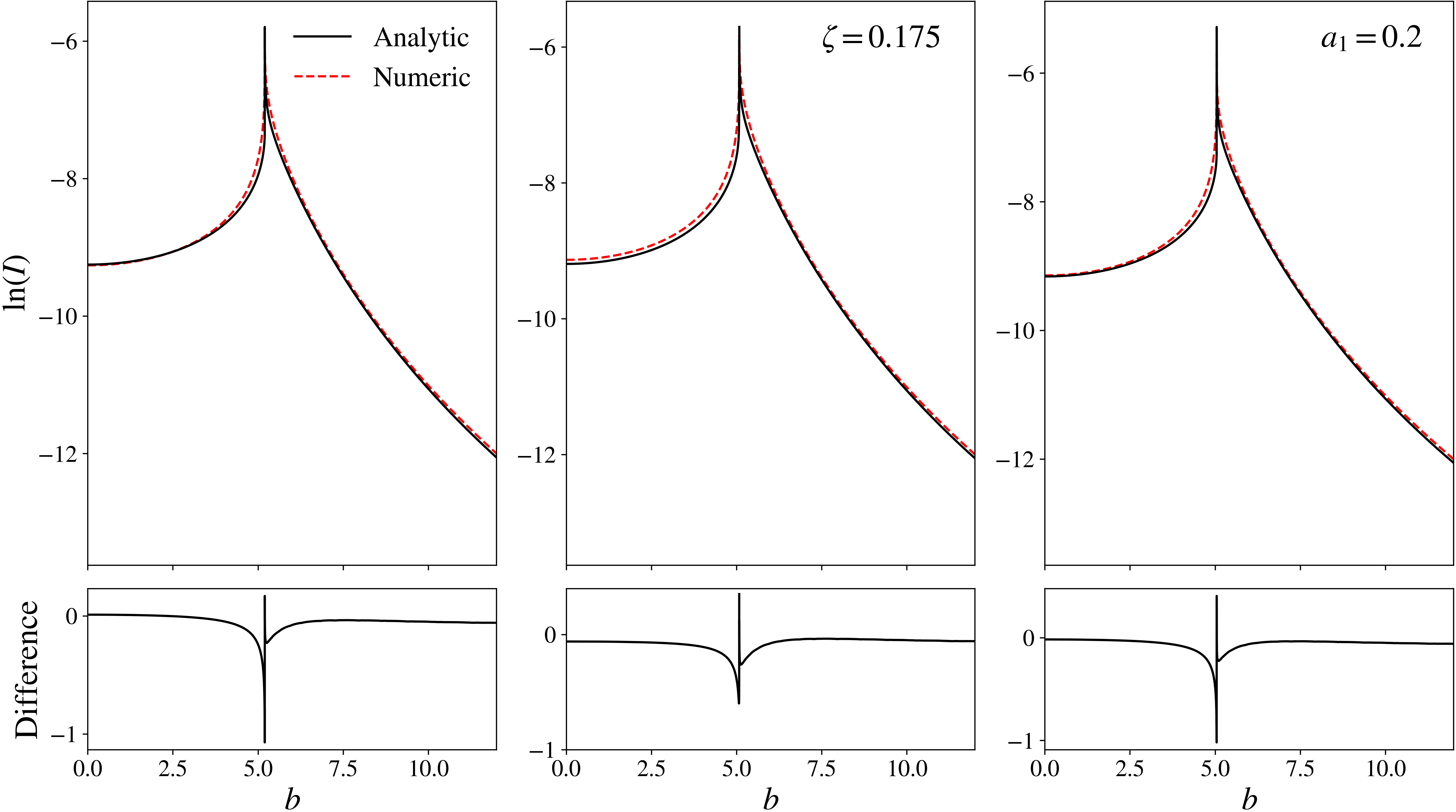
This completes the derivation for the interior of the critical curve. In Appendix A, we evaluate (58) in GR, and to first order in the coupling constants in sGB and RZ. This calculation agrees with our numerical results to striking accuracy, see Figure 6.

In the region near the critical curve (i.e., near the critical impact parameter), we derive the intensity profile generically using the following strategy. We evaluate the integral (49) by forming an expansion of the frame invariant emissivity, $J(\lambda)$, around the affine parameter which corresponds to the radius of closest approach, $\lambda_{min}$, such that $r(\lambda_{min})=r_{min}$. Then, by exploiting the fact that $J(\lambda)$ can be well approximated by a Gaussian curve peaked at a point of maximum emission, (see Figure 5 for different choices of $b>b_{c}$), we integrate (49) analytically using Laplace’s method.

We begin our derivation by writing expansions about $\lambda_{min}$ for the radial profile $r(\lambda)$ and the photon four momentum $k_{\mu}(\lambda)$. Note that for each null ray outside of the photon sphere there exists a unique radius of closest approach, $r_{min}$. Furthermore, since each spacetime we consider is spherically symmetric, the path taken from $r\gg r_{min}$ to $r_{min}$ must be identical to that taken from $r_{min}$ to $r\gg r_{min}$. This implies that $r(\lambda)$ is an even function of the affine parameter about $\lambda_{min}$. Allowing $r(\lambda_{min})=r_{min}$, it follows that, to lowest order in $(\lambda-\lambda_{min})$ we can approximate $r(\lambda)$ as

Again exploiting time and azimuthal translation symmetries allows us to write $k_{\mu}=(-E,k_{r}(\lambda),0,bE)$. It immediately follows from (59) that the radial component of the photon four momentum is linear in $(\lambda-\lambda_{min})$, i.e.,

Note that, given (59) and (60), the limit $\lambda\to\lambda_{min}$ is equivalent to taking $r\to r_{min}$ and $k_{r}\to 0$.

To solve for $d^{2}r(\lambda)/d\lambda^{2}$ and $dk_{r}/d\lambda$ at $\lambda=\lambda_{min}$, we use the null condition, $k_{\mu}k^{\mu}=0$. Expanding the null condition, we find that

Evaluating (61) in the limit of $\lambda\to\lambda_{min}$, we recover

We now use (61) to solve for $dk_{r}(\lambda)/d\lambda$ at $\lambda=\lambda_{min}$ by differentiating (61) with respect to the affine parameter and evaluating at $\lambda=\lambda_{min}$, which results in

where we have used (62) to simplify (63) and defined

We now raise the index of (63) to find

Equations (63) and (65) allow us to evaluate the frame dependent emissivity (27) and the frequency, $\nu=-k_{\mu}u^{\mu}$. Using (65) in (27) and expanding around $\lambda_{min}$, we have

Using (63) we find that, to lowest order in $(\lambda-\lambda_{min})$, the frequency is given by

where

Note that in (67) we have neglected second order contributions to the frequency because the frame invariant emissivity, $J$, goes as $J\sim\nu^{-2}$, making any $\mathcal{O}[(\lambda-\lambda_{min})^{2}]$ terms too high order to contribute to the final calculation.

We now use (66) and (67) in (4), to find that the invariant emissivity can be expanded to second order in $(\lambda-\lambda_{min})$ as

References

- Bardeen (1973) Bardeen, J. M. 1973, Black Holes (Les Astres Occlus), 215
- Campbell et al. (1992) Campbell, B. A., Kaloper, N., & Olive, K. A. 1992, Physics Letters B, 285, 199. doi:10.1016/0370-2693(92)91452-F
- Cárdenas-Avendaño et al. (2019) Cárdenas-Avendaño, A., Godfrey, J., Yunes, N., et al. 2019, Phys. Rev. D, 100, 024039. doi:10.1103/PhysRevD.100.024039
- Chaverra & Sarbach (2015) Chaverra, E. & Sarbach, O. 2015, Classical and Quantum Gravity, 32, 155006. doi:10.1088/0264-9381/32/15/155006
- Collins & Hughes (2004) Collins, N. A. & Hughes, S. A. 2004, Phys. Rev. D, 69, 124022. doi:10.1103/PhysRevD.69.124022
- Glampedakis & Pappas (2021) Glampedakis, K. & Pappas, G. 2021, arXiv:2102.13573
- Gourgoulhon (2006) Gourgoulhon, E. 2006, EAS Publications Series, 21, 43. doi:10.1051/eas:2006106
- Gralla (2021) Gralla, S. E. 2021, Phys. Rev. D, 103, 024023. doi:10.1103/PhysRevD.103.024023
- Gralla et al. (2020) Gralla, S. E., Lupsasca, A., & Marrone, D. P. 2020, Phys. Rev. D, 102, 124004. doi:10.1103/PhysRevD.102.124004
- Johannsen et al. (2016) Johannsen, T., Broderick, A. E., Plewa, P. M., et al. 2016, Phys. Rev. Lett., 116, 031101. doi:10.1103/PhysRevLett.116.031101
- Johnson et al. (2020) Johnson, M. D., Lupsasca, A., Strominger, A., et al. 2020, Science Advances, 6, eaaz1310. doi:10.1126/sciadv.aaz1310
- Kanti et al. (1996) Kanti, P., Mavromatos, N. E., Rizos, J., et al. 1996, Phys. Rev. D, 54, 5049. doi:10.1103/PhysRevD.54.5049
- Kocherlakota et al. (2021) Kocherlakota, P., Rezzolla, L., Falcke, H., et al. 2021, Phys. Rev. D, 103, 104047. doi:10.1103/PhysRevD.103.104047
- Lara et al. (2021) Lara, G., Völkel, S. H., & Barausse, E. 2021, arXiv:2110.00026
- Maselli et al. (2015) Maselli, A., Pani, P., Gualtieri, L., et al. 2015, Phys. Rev. D, 92, 083014. doi:10.1103/PhysRevD.92.083014
- Narayan et al. (2019) Narayan, R., Johnson, M. D., & Gammie, C. F. 2019, ApJ, 885, L33. doi:10.3847/2041-8213/ab518c
- Psaltis et al. (2020) Psaltis, D., Medeiros, L., Christian, P., et al. 2020, Phys. Rev. Lett., 125, 141104. doi:10.1103/PhysRevLett.125.141104
- Rezzolla & Zhidenko (2014) Rezzolla, L. & Zhidenko, A. 2014, Phys. Rev. D, 90, 084009. doi:10.1103/PhysRevD.90.084009
- Shapiro & Teukolsky (1983) Shapiro, S. L. & Teukolsky, S. A. 1983, A Wiley-Interscience Publication, New York: Wiley, 1983
- The Event Horizon Telescope Collaboration (2019a) The Event Horizon Telescope Collaboration, 2019a, Astrophysical Journal Letters, 875, L1
- The Event Horizon Telescope Collaboration (2019b) The Event Horizon Telescope Collaboration, 2019b, Astrophysical Journal Letters, 875, L2
- The Event Horizon Telescope Collaboration (2019c) The Event Horizon Telescope Collaboration, 2019c, Astrophysical Journal Letters, 875, L3
- The Event Horizon Telescope Collaboration (2019d) The Event Horizon Telescope Collaboration, 2019d, Astrophysical Journal Letters, 875, L4
- The Event Horizon Telescope Collaboration (2019e) The Event Horizon Telescope Collaboration, 2019e, Astrophysical Journal Letters, 875, L5
- The Event Horizon Telescope Collaboration (2019f) The Event Horizon Telescope Collaboration, 2019f, Astrophysical Journal Letters, 875, L6
- Völkel et al. (2020) Völkel, S. H., Barausse, E., Franchini, N., et al. 2020, arXiv:2011.06812
- Yunes & Stein (2011) Yunes, N. & Stein, L. C. 2011, Phys. Rev. D, 83, 104002. doi:10.1103/PhysRevD.83.104002