Local Structure and effective Dimensionality of Time Series Data Sets
Abstract.
The goal of this paper is to develop novel tools for understanding the local structure of systems of functions, e.g. time-series data points, such as the total correlation function, the Cohen class of the data set, the data operator and the average lack of concentration. The Cohen class of the data operator gives a time-frequency representation of the data set. Furthermore, we show that the von Neumann entropy of the data operator captures local features of the data set and that it is related to the notion of the effective dimensionality. The accumulated Cohen class of the data operator gives us a low-dimensional representation of the data set and we quantify this in terms of the average lack of concentration and the von Neumann entropy of the data operator and an improvement of the Berezin-Lieb inequality using the projection functional of the data augmentation operator. The framework for our approach is provided by quantum harmonic analysis.
1. Introduction
For high-dimensional, complex data sets, structured dimensionality reduction methods are essential in order to enable useful further processing[27]. The guiding idea behind some approaches is the hypothesis, that successful (machine) learning is made possible by the fact that data of interest live on low-dimensional manifolds as opposed to the dimensionality of the space in which the data are collected a priori. Inspired by this idea, the approach envisaged in this article hinges on the idea that the dimension of data is not at all canonical, but can vary according to the chosen representation of the data. Ideally, the choice of representation avoids loss of essential information. While image data are directly accessible and rather easy to interpret, time series data such as audio seem to be harder to understand, cluster and classify. Time-frequency (TF) methods are often applied to obtain image-like representations of time-series data such as speech and music [19], and to encode the impact of variance over time, [12, 13, 5, 14]. Applying convolutional neural network (CNN) architectures to the resulting TF-transformed versions of time-series data points has been surprisingly successful in various machine learning (ML) tasks. The underlying processes are, however, not entirely understood. One important hypothesis is the assumption that the informative content of the data actually lies on a manifold of significantly lower dimensions than their domain. It is not clear, however, how these essential parts of data can be made explicit.
In the work presented in the current article, we take a stance toward the identification of time-frequency localized components that determine the entropy of a data set. In particular, certain intrinsic structures, which repeat over a data set of interest, may be encoded as TF-local components. TF-local signal components, which repeat over the data points in a data set, probably play a crucial role in training realizations of a given CNN architecture based on specific data sets [11, 8]. Intuitively, these components determine the coefficients of the convolutional kernels in the lower levels of the network and thus can be expected to carry the essential structure for a certain problem at hand.
While on the one hand, the random choice of convolution coefficients can lead to improved stability to small perturbations [31] and also give guaranteed reconstruction properties [26], random initialization of all coefficients still is not always a good strategy and may not lead to a favorable architecture realization [18]. Careful investigation of the interaction between structures present in the data and the impact of convolutions in lower levels of CNNs is thus necessary to better understand the observed phenomena.
In this work, we make a connection between the ubiquitous local averaging of TF-representations of signals in a given data set, data augmentation of original time-domain data and their effective dimensionality [28] (ED) via tools from quantum harmonic analysis developed in [23, 24, 25]. The key insight guiding these efforts is the association of the data operator to a system of functions . This allows us to capture the structure of the data and their interaction. Data augmentation is then formalized as the mixed-state localization operator corresponding to . The data operator is the analogue of the density operator in quantum statistical mechanics. This connection leads us to the investigation of various notions of quantum entropies as well as their implications for the structure of the functions in and the properties of their interactions. Our results demonstrate that the von Neumann entropy is well-adapted to quantification of the (augmented) data set’s entropy via von Neumann entropy of the data density operator . Von Neumann entropy, in turn, is closely related to effective dimensionality, which was introduced in order to describe the underlying structural properties of a data set as opposed to its a priori dimension.
Our approach uses tools such as mixed state localization operators and the accumulated Cohen’s class of an operator, which have recently been developed in [24, 25] in work aimed to connect time-frequency analysis and quantum harmonic analysis [29]. Furthermore, new notions, such as the total correlation function, which captures local time-frequency correlation between the different data points, and an average loss of concentration, encoding the interaction between data structure and augmentation, are introduced. In the context of data analysis and the desire to obtain reasonable information by dimensionality reduction, understanding the smoothing action of augmentation, is formalized.
Our manuscript is divided into two parts: In Part A we outline the main ideas and results. We illustrate the connections to and implications for data analysis with the help of various examples. In Part B we put forward the theoretical background concerning quantum harmonic analysis, von Neumann entropy, an improvement of the Berezin-Lieb inequality for the data augmentation operator and introduce novel notions connecting data analysis and quantum harmonic analysis. Our sharpening of the Berezin-Lieb inequality for the data augmentation operator involves the projection functional that measures how much the data augmentation operator fails of being a projection. In the final statement, the projection functional is replaced by the average lack of concentration which is more suited for our purposes. The proofs of the main results make use of these techniques.
2. Part A: Context, Results and Numerical Examples
2.1. Concepts and Notation
2.1.1. Data sets and data operators
A data set is a collection of data points in a certain fixed vector space with innerproduct, whose properties are not further specified at this point. For two data points , their tensor product is an operator acting on , defined by
| (1) |
We define, for a given data set the following data operator:
| (2) |
As our normalization, we will always assume that , equivalently that .
Remark 1.
If , then is the empirical covariance operator for the multivariate distribution of the hypothetic underlying density generating the data set. While stationary processes are characterized by their spectral density, more complex processes may be described by the singular values of their covariance operator, which are closely related to the Karhunen-Loeve transform.
In data analysis, Karhunen-Loeve transform is also known as principal component analysis and is defined as follows. Since is a self-adjoint operator, it possesses an orthogonal basis of eigenvectors , with corresponding eigenvalues , such that
| (3) |
We note here, that the eigenfunctions of maximize the following expression:
| (4) |
which, for the data operator , takes the form
| (5) |
2.1.2. Effective dimensionality
We define the entropy of a given data set as the von Neumann entropy of the associated data operator :
| (6) |
The case of maximal correlation (all data points are scalar multiples of a single data point) corresponds to , thus increasing can be interpreted as a decrease in the correlations within the data.
Remark 2.
- •
In [28], Roy and Vetterli proposed a concept they denoted as effective dimensionality, also cf.[17] which is based on the Shannon entropy of singular values of a given matrix, which may be thought of as the collection of data points. Since their concept is closely related to our understanding of entropy of a data set as given in (6), we adopt their notion of effective dimensionality of as a synonym for the underlying data set’s entropy.
- •
The tools of quantum information theory allow us to give a more operational interpretation of the statement that an increase in corresponds to a decrease in correlation. Each of the operators for describes a quantum state, and we consider the following experiment: Alice picks a quantum state at random from these states (with equal probability for each state), and sends it to Bob. Bob knows the data set , but not which particular state was sent by Alice. He therefore measures some observable in the state in order to deduce which of the states , he received. Holevo [20] has shown that an upper bound for the information Bob can deduce about which state he received is given by . In other words, quantifies how difficult it is to tell the operators apart. We consider a data set to be correlated if the operators are difficult to tell apart, in other words if the maximum information accessible to Bob is small. Of course, notions such as accessible information and measurement of an observable can be made precise, and we refer to Chapter 11 of [30].
2.1.3. Time-frequency analysis, correlation and local averaging
For time series data of various origins, it turns out that characteristics which may in principle be captured by Fourier analysis, that is, which are appropriately represented by analysing their spectral content, change over time. Furthermore, correlations are observed over both time and frequency; which means that components which are localised in time and frequency repeat, up to small disturbances and modifications, over the entire signal. In order to capture these intrinsic structures, more often than not, time-series are processed by means of some methods from time-frequency (TF) analysis before being exploited by machine learning (ML) methods. TF methods such as the short-time Fourier (STFT) or wavelet transform yield a two-dimensional representation of a hitherto one-dimensional data point.
The respective pre-processing is supposed to extract time-frequency structure of the signal which is believed to be essential to human perception, and introduces invariance to phase-shifts. Most commonly, the first processing step consists of taking a short-time Fourier transform
| (7) |
followed by a non-linearity in the form of either absolute value or absolute value squared.
Remark 3.
We will subsequently use the notation for . The operator is called a time-frequency shift by .
For a data point one thus obtains a first feature stage as follows
| (8) |
for some window function .
Due to the structure of the convolutional layers in a CNN, the first, non-linearly generated feature, undergoes local weighted averaging in the next and a few subsequent layers. Assuming several weights, also called convolutional kernels, which are all supported in a compact set , we obtain the output of the first convolutional layer:
The consecutive local averaging steps applied in CNNs are crucial in making CNNs effective for many ML problems. It is the main goal of this work to explain the impact of local TF-averaging on entropy, which encodes the correlation between data points.
Remark 4.
When considering a large data set, only functions , which are correlated in the sense of (5) with several or many data points will get the chance to have a significant eigenvalue. Considering, additionally, the orthogonality condition, it seems reasonable to assume that the correlation takes place in local components, which repeat over . While different expansions are possible, we consider an expansion of the data points in a (tight) Gabor frame, that is:
| (9) |
The expansion coefficients of will be
interpreted as TF-coefficients, since, for an appropriately localized
window , they encode the TF-local energy of at a point
in phase-space.
Writing an arbitrary similarly as
, (5)
takes the form
| (10) |
which may be interpreted, by ignoring the smoothing factor , as finding the vector of TF-coefficients which are maximally correlated, on average and in a TF-sense, with the TF-coefficients of the data.
In order to capture the over-all time-frequency correlation structure in a data set , we introduce the following total correlation function
| (11) |
Example 2.1.
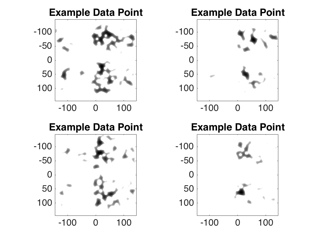
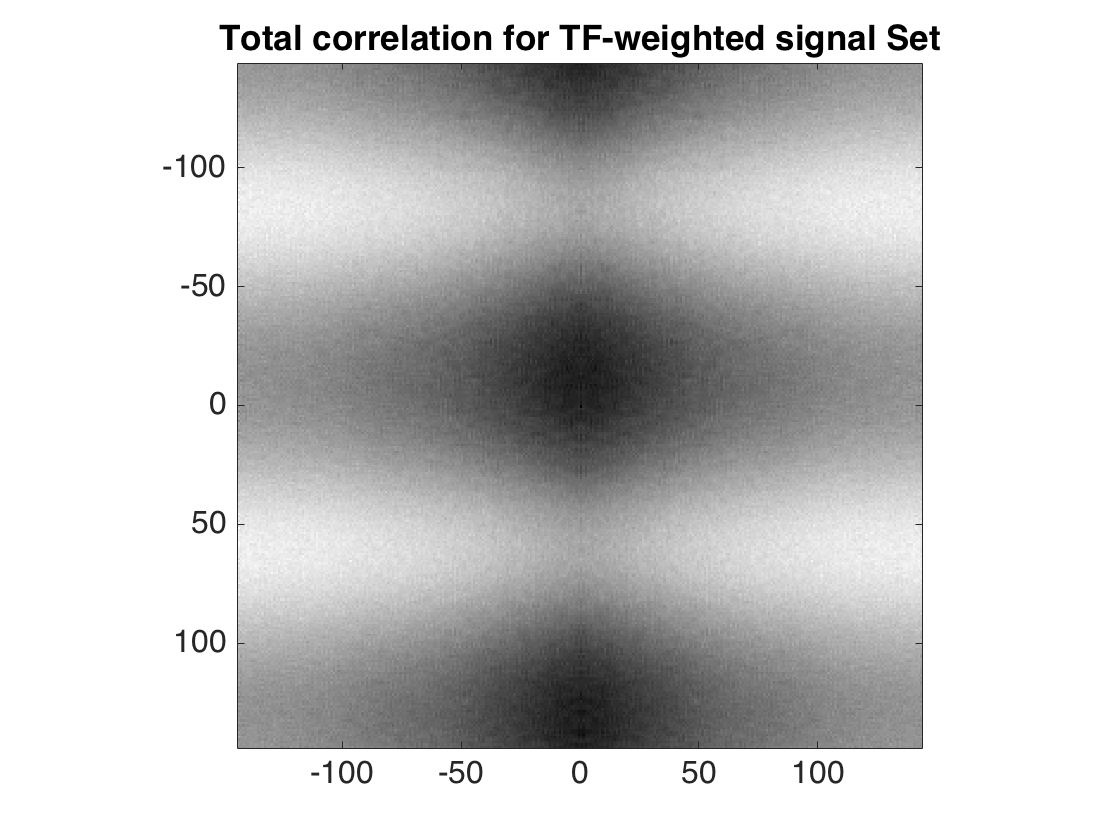
As an example, we compute the total correlation of a data set of signals
with random TF-coefficients and common TF-weight. More precisely, the data points are given as in (9), with uniformly distributed coefficients , to which a common weight
is applied, so that the actual data points are given by
.
Four example data points are shown in
Figure 1, (a), and the data set’s total correlation function is plotted in Figure 1, (b). The total correlation captures the TF-behaviour characterized by the weight , as expected.
2.1.4. Data augmentation
Data augmentation is a method commonly used in data analysis. Its aim is first to increase the amount of available data by adding carefully modified versions of data points to existing data, which allows for the usage of larger network architectures. Augmentation often is conducted by applying certain operators to the elements in . Second, the particular choice of the operators leads to the enhancement of desirable invariances of the resulting network, whose parameters are learnt from the augmented data set. An example in image processing would be the addition of rotated versions of images in the situation of object classification. In the context of audio data, it is reasonable to assume that small TF-shifts have no effect on substantial properties of the data. We next give a definition of TF-data augmentation for a set of TF-sampling points .
Definition 2.1 (-augmentation).
For a data set and a compact set , its -augmentation is defined by
The operator corresponding to the augmented data set is then given by
| (12) |
In Section 3.1.1, we introduce the concept of mixed-state localization operators [24]. Their definition is based on operator convolutions, which will be formally introduced in Definition 3.2. It turns out, that the mixed-state localization operator corresponding to the data operator of a data set is precisely the operator corresponding to the -augmented data set , . In other words, using the notation from Definition 3.2, in accordance with (16) we will also write
| (13) |
Remark 5.
In machine learning, data augmentation is obviously based on a finite and discrete set of time-frequency shifts, or in fact, any other set of operators which are expected to not influence the data points characteristics in such away that, e.g. class membership changes.
We give some examples in order to illustrate how the mixed-state localization operator corresponding to a data set captures information on the data set itself as well as on the impact of averaging over a domain .
2.1.5. Simple motivating examples for the impact of augmentation
- (1)
Gaussian and Hermite functions
We first recall the case of Gaussian window , and note that we obtain, with , andthe situation of classical time-frequency localization operators, which have frequently been studied in the literature [9, 15, 10, 7, 1, 4]. In this simple situation, the interpretation of correlation with respect to the augmentation (12) becomes quite straight-forward and can be understood as follows. The total correlation function is simply the spectrogram , while the eigenfunctions of maximise the expression
(14) and thus result in an orthonormal system of functions, which are optimally correlated with the energy of TF-shifted Gaussians , for inside . The resulting function system approximates the Hermite functions, cf. [9].
- (2)
Interpolating two Hermite functions
We next investigate the interaction between two distinct states and the entropy of the resulting operator as well as its TF-augmentation. Let and be two -normalized functions and define , for . We first choose and to be the first and tenth Hermite function. In Figure 2(a), the entropies of the operators , for running from 0 to 1, that is, for the interpolation between first and tenth Hermite function are shown. Similar behaviour is observed for interpolation between other orthonormal pairs, which shows, that the entropy does not substantially depend on the TF-localization of the involved functions.
However, the entropy-behaviour of the TF-augmentations is different. We consider the interpolation between Gaussian and first Hermite function. The corresponding entropies of are depicted in Figure 2(b). We compare these results to the augmentation of the interpolation between zeroth and tenth Hermite function, depicted in Figure 2(c).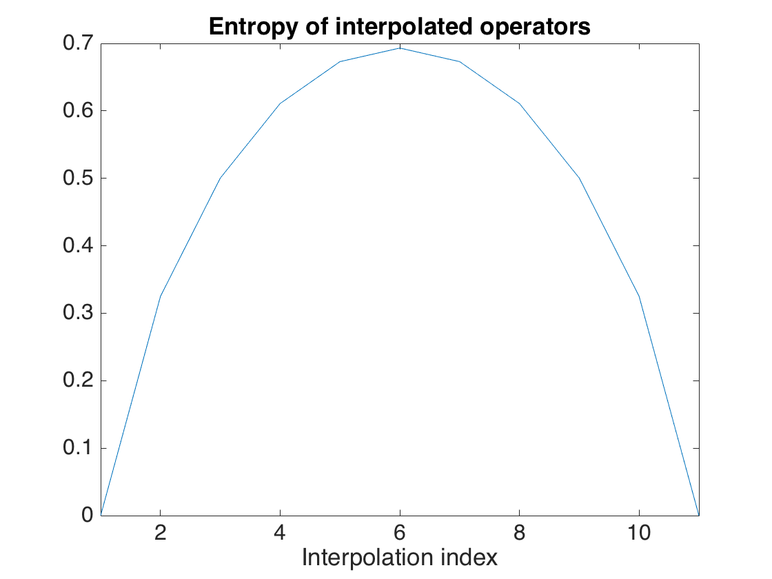
(a) Entropy 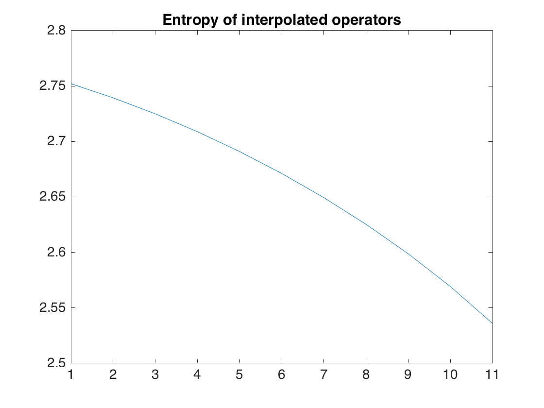
(b) Entropies of the for with the first and second Hermite function. 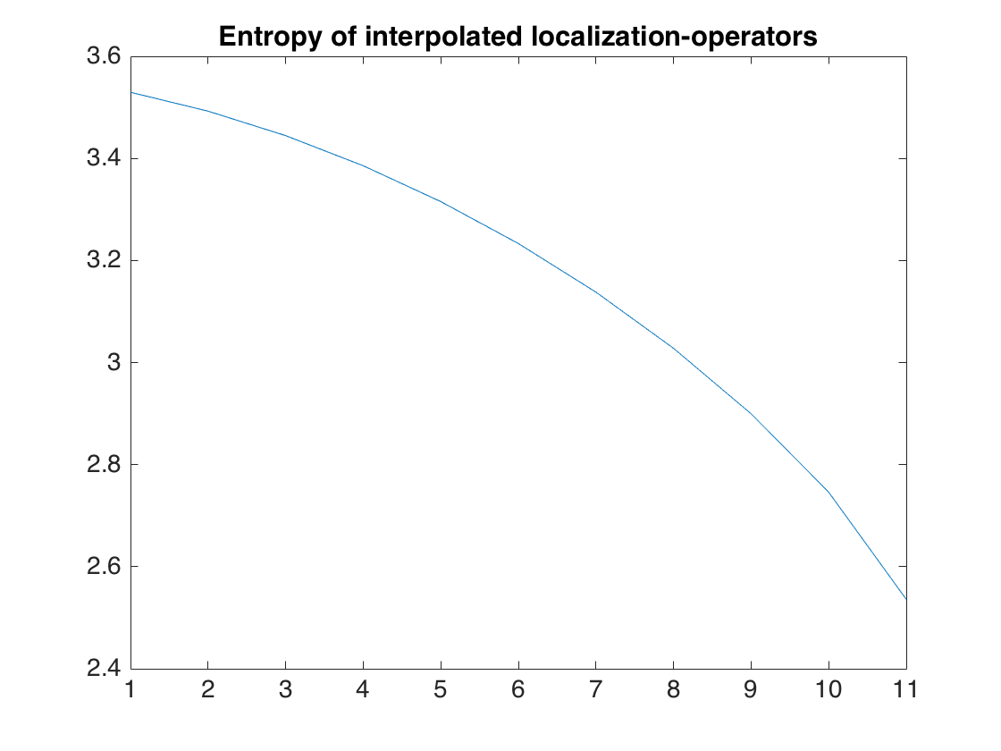
(c) Entropies of the for with the first and the tenth Hermite function . Figure 2. (a) Entropies of the , running from 0 to 1, for interpolation between first and tenth Hermite function. Similar behavior is observed for interpolation between other orthonormal pairs. (b) Entropies of the for with the first and second Hermite function. (c) Entropies of the for with the first and the tenth Hermite function . In Figure 3, the TF-behaviour of the three involved functions is illustrated by their respective spectrogram. The TF-localization of the single components plays a crucial role for the entropy of the augmented data operator: the more TF-localized the overall signal energy is within the area of augmentation , the smaller the resulting entropy. We next investigate this insight by means of a more realistic data set.

Figure 3. Spectrogram of the zeroth, first and tenth Hermite function. - (3)
Time-localized chirps
We construct a more complex data set with an inherent TF- local structure as follows. The data set consists of chirps , , with random base frequency between and (normally distributed with mean ) and envelopes given by randomly rotated Bartlett-Hanning windows, each of length in samples; see Figure 4(a) for some examples. We let vary between and and compute the rank and effective dimensionality of the corresponding data matrix . Rank grows linearly with the number of data points, saturates at the size of the matrix, that is, , and does not reflect the structure of the data set. Effective dimensionality, on the other hand, depicted in Figure 4(b) for several random realizations, remains relatively stable with respect to the size of the data set; the interpretation of this behaviour is that this measure, i.e. entropy, encodes the actual information present in the data, which can be extracted given a sufficient number of data points.
The entropies of the augmented data sets for a square of side-length 80 are shown by the dotted lines in Figure 4(b). The effective dimensionality of this data set can be extracted from fewer data points in the original data set . On the other hand, augmentation with respect to this particular significantly increases the data set’s entropy. The results in this article show that augmentation can be designed as to reduce the increase of entropy. The design of the augmentation depends on the correlation structure in the data. To see this, we also plot the total correlation for the chirp data set, in Figure 5. It is visible, that due to the restricted frequency band, correlation in frequency direction decays quickly, while, given to the uniformly distributed time-localization, correlation in time is more persistent, since also localized chirps, which are significantly separated in time can be highly correlated if they have sufficient overlap in frequency.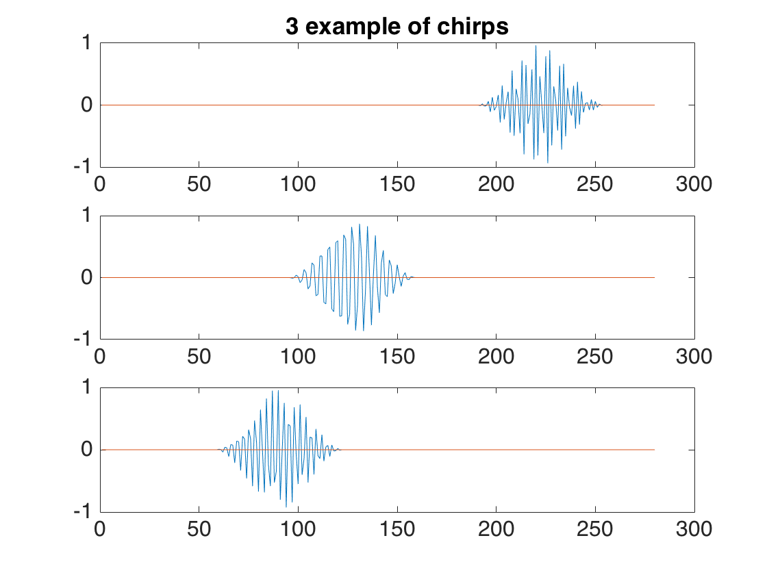
(a) Data points 
(b) Entropies Figure 4. (a) Windowed chirps (b) Effective dimensionality of data operator for the chirp data set and its -augmentation. Entropy of the augmented data set is dotted. Note that for the latter, the data operator has full rank even for a single data point. 
Figure 5. Total Correlation for Data set of windowed chirps
In the interpretation of the local correlation in data points, we now deal with the following hypothesis: if is highly locally correlated in (e.g. weakly TF-shifted Gaussian windows), then augmentation by will not increase its entropy significantly, and a small number of eigenfunctions of represents the augmented data set well. Our main results, which we present next, give insight into the relation between a data set, its augmentation by and the domain .
2.2. Main Results
The effective dimensionality of the augmented data set, represented by the operator , depends on the original data set represented by , on the domain , and crucially on the interaction between and . This interaction reflects the presence of local correlations in the data set, that is, the presence of signal structures which, up to small TF-shifts, repeat over .
Understanding the relation between the effective dimensionality of and the pair is an important goal of this paper. In particular, since the effective dimensionality of the augmented data set is defined rather abstractly as the von Neumann entropy of an operator, we aim to understand this abstract object in terms of certain auxiliary concepts whose interpretations are less obscure.
One such concept is the already introduced total correlation function
when
which encodes the TF-correlations in the data set. In fact, assume a TF-representation of each as suggested in (9) and write , then
This, by assuming , shows that
encodes TF-local
correlations for small . The slower decays, the
more TF-distant correlations must be expected over the data set.
Of course, only gives information regarding the (non-augmented)
data set
described by . To describe its interactions with ,
introduced by the augmentation, we, therefore, propose a new concept called
the average lack of concentration,
defined by
It turns out that these quantities allow us to give lower and upper bounds for the abstract quantity of effective dimensionality of the augmented data set. In the next theorem, which is Theorem 3.7, denotes differential entropy of a probability distribution on defined by
Theorem.
For compact and a positive trace class operator with , the following inequalities hold:
2.2.1. Approximation of augmented data operator
We will also give an approximation of the augmented data operator by its eigenvectors, and approximation quality is quantified by the average lack of concentration. As we will see, for a compact domain and a density operator the mixed-state localization operator has a diagonalization
where are the eigenvalues of with eigenfunctions and
We further let and define
then we may approximate by . The approximation quality depends on the correlation properties of , as measured by , and the interaction of correlations and , as measured by the average lack of concentration. In the last inequality we decouple the influence of the correlations and the domain to obtain an upper bound in terms of the size of the perimeter of .
Theorem.
For compact and a positive trace class operator with , let where . Then
As our first theorem shows that we can bound from above using , we can easily get an upper bound in terms of as well. We observe that the quality of approximation of the augmented data set by its principal components is entirely determined by the interaction between the original data set’s total correlation and the augmentation characteristics. Several examples will enlighten the connection in the following section.
2.3. Examples and Numerical Illustrations
2.3.1. Simple motivating examples revisited
We return to the examples from Section 2.1.5 in order to interpret the results on effective dimensionality and ALC for the simple data sets presented there.
- (1)
Gaussian functions and their linear combinations
We first consider a set of data points generated by a small family of time-frequency shifted Gaussian windows as followswith random coefficients and time-frequency coordinates randomly chosen in a rectangular domain , which is symmetric about in both time and frequency direction, more precisely, of size .
We then compare the average lack of concentration to the effective dimensionality of the data set generated by augmentation of with respect to different domains , where shape and size of is allowed to vary during the experiment. More precisely, is quadratic (), is a a wide rectangle of size and is a narrow rectangle of size ; each of the domains has thus initially size approximately and whose side-lengths enlarged in a second and third step by a factor of and , respectively. This yields yield sizes of approximately and , respectively. The results of trials are shown in Figure 6, where the mean of each experimental setup is shown together with the variance. It is obvious that the effective dimensionality grows with the size of the augmentation domain. On the other hand, , whose shape is adapted to the correlation structure of the data set, leads to lower entropies than the other two choices of . This effect is also reflected in the ALCs. The relation between ALC and ED is further studied in the following example.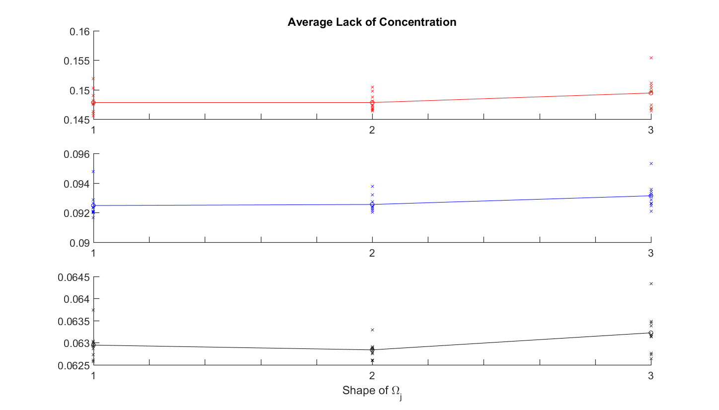

Figure 6. Effective Dimensionality and ALC for data set linear combinations of shifted Gaussian windows and varying shape and size of the localization domains , : is quadratic (), is a narrow rectangle of size and is a wide rectangle of size ; each of the domains has thus size approximately , upper plots. Each of the localization domains is then enlarged by a factor of and , respectively, to yield a size of approximately and , respectively. The resulting ALCs and EDs are shown in the middle and lower plots. Each experiment was repeated 100 times, shown are mean (o) and variance (x). 

Figure 7. Effective Dimensionality and ALC for data set of windowed chirps and varying shape and size of the localization domains , : is quadratic (), is a narrow rectangle of size and is a wide rectangle of size ; each of the domains has thus size approximately . Each of the localization domains is then enlarged by a factor of and , respectively, to yield a size of approximately and , respectively. Each experiment was repeated 100 times, shown are mean (o) and variance (x). 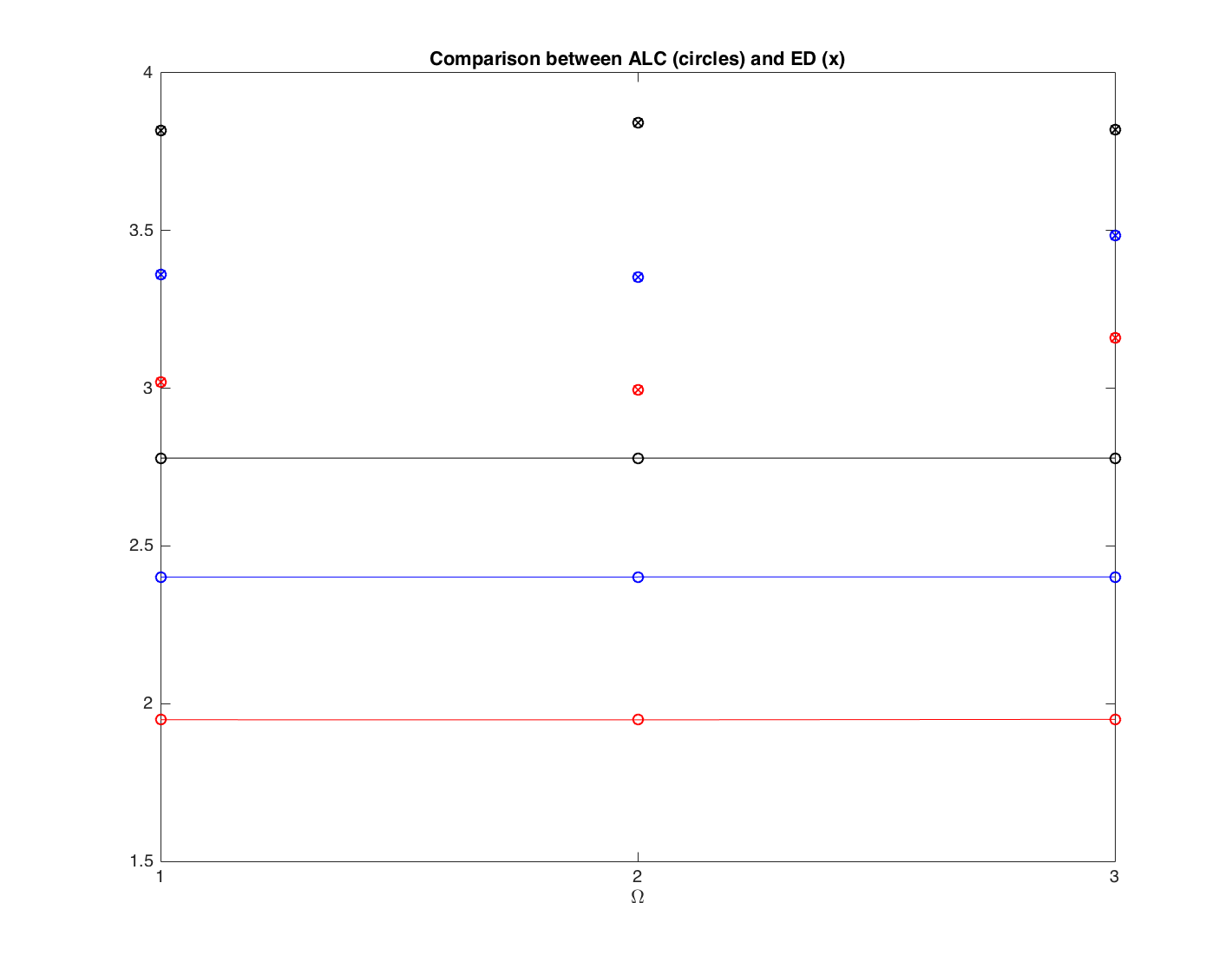
Figure 8. Comparison of Effective Dimensionality ( and for data set of windowed chirps and varying shape and size of the localization domains , : is quadratic (), is a narrow rectangle of size and is a wide rectangle of size ; each of the domains has thus size approximately (red values). Each of the localization domains is then enlarged by a factor of and , respectively, to yield a size of approximately (blue values) and (black values), respectively. - (2)
Time-localized chirps
We study the data set of time-localized chirps, which was introduced in Section 2.1.5. For the subsequent experiments, data points, generated as described in Section 2.1.5, were used. In Figure 5 we see that total correlation is concentrated in a region which is eccentric with respect to time- and frequency axis. That is, is better concentrated in frequency direction than in time. We calculate and for both quadratic and rectangular domains of varying eccentricity and approximately constant size as in Experiment (1) above.
As expected, the shape of influences ALC and thus effective dimensionality of the augmented data set. Results are shown in Figure 7 for the three different domains , . Figure 8 illustrates the result of Theorem 3.7 in more detail, by comparing, for the same experimental setup, the values of and . The illustration of the Theorem’s result is obvious; this example makes the relation between the shape of the domain of augmentation, its size and the total correlation of more precise.
2.3.2. A data set of local components
In this example, we consider a given signal , whose over-all energy is assumed well-concentrated within . A data set is generated by data points defined as
| (15) |
for with and an orthogonal noise component , such that .


The data set is first generated without noise component and augmented with respect to a quadratic domain of size . In Figure 9, the eigenvalues of the resulting mixed-state localization operators are shown. We see that adding several close Gaussian windows does not significantly change the augmented data set’s entropy: for the standard localization operator it is , while for a data set of TF-shifted Gaussians it is , see Figure 9(a). This is intuitively clear, since the overall total correlation remains concentrated inside . The situation starts to change, as soon as the local components explain only part of the data structure, that is, the energy in the noise part of each data point increases, hence the total correlation is not exclusively concentrated inside . The resulting eigenvalues are depicted in see Figure 9(b). Level 1 noise has carries approximately and Level 2 noise of the signal energy.
2.3.3. The mix of local and global influence
This final example illustrates the impact of the TF-characteristics of each data point, the interaction between local TF-components and their influence on a data set’s entropy. We consider Hermite functions and distinguish two cases of related data sets in order to under the influence of the growing TF-spread of Hermite functions , . To this end, we consider the rank-one operators , which correspond to the data sets , , and compare them to , corresponding to . We compute the entropy of the augmented data sets and , for a square of size . The second setup, i.e. the augmentation of , actually yields smaller entropy of the corresponding mixed-state localization operator than see Figure 10. This example shows that augmentation of smaller data sets may lead to higher effective dimensionality than augmentation of a data set with more data points, even if those are orthogonal. At closer inspection, this is not a surprising result, since the decay of the eigenvalues of is faster and thus the ALC of is smaller than for . In the context of data augmentation this means that the augmentation is adapted to the correlation structure of rather than to that of . Hence, for augmentation changes the information in the data set more significantly than for , for which the overall, average correlation is better concentrated inside .

2.4. Interpretation and perspectives
In the previous section, we presented several data sets of structured time-series data in order to illustrate the main results given in Section 2.2. The given examples show an intricate connection between TF-localized correlations in the signals contained in a given data set and the effect of augmentation. It is interesting to observe, that augmentation, which is used as a means to improve generalization properties of networks learned from data, leads to varying effects in dependence on the TF-structure of the original data set. In particular, if the structure of the set is aligned with the area of local correlations within the data set, the consequence of augmentation on the effective dimensionality is limited. Exploiting this observation, data augmentation can be designed in order to increase the size of a data set without changing its intrinsic structure. On the other hand, preliminary experiments show the potential of adapted augmentation, in order to separate signal classes with distinct correlation properties. The details and applicability of this idea will be elaborated in future work.
3. Part B: Technical Details and Proofs
3.1. Technical Background
As a theoretical framework for our mathematical results, we will use the theory of quantum harmonic analysis first introduced by Werner in [29]. This framework allows us to exploit intuitions and results from harmonic analysis of functions, such as convolutions, to prove results that apply to both operators and functions.
3.1.1. Convolutions
For our purposes, the most important concept from quantum harmonic analysis is that of convolutions of operators and functions. To introduce these operations, we first define a time-frequency shift of an operator as follows.
Definition 3.1 (Shift of operator).
Given an operator on , we define its translation to be the operator
where denotes the time-frequency shift of by , .
Using this translation operation, we can define two new convolution operations:
Definition 3.2 (Operator convolutions).
- (1)
Let and let be a trace class operator on . The convolution is the operator on defined by
interpreted either as a Bochner integral or in the weak sense:
- (2)
If are trace class operators on , the convolution is the function on defined by
where for .
We will soon restrict our attention to certain classes of functions and operators, where more insight can be gained about these convolutions, but the reader should already note that the convolution of a function with an operator yields a new operator, while the convolution of two operators yields a new function.
Now assume that is a positive trace class operator with (a so-called density operator), and for some compact subset . The convolution is then the mixed-state localization operator
| (16) |
that we already met when discussing augmentation in (12) — in that case was a data operator from (2). In other words, -augmentation can be described as a convolution operation.
The total correlation function, which we met in (11) when was a data operator, also has a simple description as a convolution, namely:
Of course, this expression for makes sense for any trace class operator , but we will mainly consider when is a data operator.
3.1.2. Properties of the convolutions
The convolutions introduced above share many properties of the usual convolution of two functions. They are both commutative and associative, and in particular the associativity is a non-trivial and useful property. As an example, we have the relation
where denotes the familiar convolution of functions. When inspecting this equation we see that it shows the compatibility of three different convolutions: of two functions, of two operators and of a function with an operator.
We summarize some other properties of the convolutions in the following proposition. Proofs can be found in [29] or [23].
Proposition 3.1.
Let .
- (1)
(Young’s inequality) For any and we have that
where is the trace class norm.
- (2)
with
- (3)
.
- (4)
If , then
- (5)
If are positive operators, then is a positive function.
- (6)
If is a positive function and is a positive operator, then is a positive operator.
Versions of the so-called Berezin-Lieb inequalities have been shown to hold in quantum harmonic analysis by different authors [29, 22]. Since none of the existing formulations in the literature cover the case we are interested in explicitly, we give a proof for completeness. The proof is essentially that of [22]. Note that our assumptions are chosen according to our needs rather than to obtain the most general statement.
Proposition 3.2 (Berezin-Lieb inequalities).
Let be a non-negative, concave continuous function on , and let be a positive trace class operator with . If is a positive compact operator on with , then
| (17) |
where is defined by the functional calculus. If is a positive function with , then
| (18) |
Proof.
We can use the spectral theorem for self-adjoint compact operators to write in terms of its eigenvalues and eigenfunctions by
By the linearity of the convolutions, we find that
where the last equality follows from expanding the definition of the convolution . Now note that for each fixed , the sequence is a probability distribution over : it is positive for each as is a positive operator, and the sequence sums to as is an orthonormal basis for each since is unitary, so that
Hence we can apply Jensen’s inequality for concave functions to get that
Note that we stay within the domain of : by Proposition 3.1, for all , and as . Also note that by the same proposition
So by integrating the inequality above and changing the order of the sum and integral, we get
Turning to the second inequality, we will use the spectral theorem to write the positive trace class operator in terms of its eigenvalues and eigenfunctions by
Since Proposition 3.1 gives that
the eigenvalues belong to the domain of and
and in particular
This means that
Now note that for each fixed , the function is a probability distribution over : it is non-negative by the positivity of and . So we can apply Jensen’s inequality to get
∎
When we pick to be a rank one operator , the associated mixed-state localization operator is a kind of operator that has been studied extensively in the field of time-frequency analysis, namely a localization operator. By writing out the definition of the convolution, we find that
3.1.3. Entropy
We have introduced the essential dimension of as the von Neumann entropy . This definition applies the function to the operator using the so-called functional calculus, but an equivalent definition is that
where are the eigenvalues of from (3). This is simply the Shannon entropy of the sequence of eigenvalues of .
As we will also be working with functions on , we will also need the differential entropy of a probability distribution on , i.e. a positive function with . The differential entropy is then
3.1.4. Convolutional neural networks and data operator
Time-series such as audio data are routinely pre-processed before being used as input to CNNs. The pre-processing steps extract time-frequency structure of the signal which is essential to human perception. Thus, the pre-processing also introduces invariance to phase-shifts. Most commonly, the first processing step consists of taking a short-time Fourier transform, cf. (7) followed by a non-linearity in the form of either absolute value or absolute value squared. For an input signal one thus obtains a first feature stage as given in (8). Due to the structure of the convolutional layers in a CNN, the output of the first convolutional layer can then be written as
and these equalities offer various different interpretations of the first convolutional layer’s output. First, we can obviously interpret the value at each as the correlation between the TF-localization operator applied to with . This operator itself, then, is simply the TF-shifted version of . More interestingly, we may equally consider the operator , which now depends on the data points. Ideally, the can be chosen as to optimally enforce correlation within data classes and to separate, or de-correlate, data points from different classes.
In order to isolate and investigate the question of correlations between data points, we generalize the rank-one operator to the sum over all data points, thus considering and the corresponding mixed-state localization operator , which actually represents the local time-frequency averages of the data-points . In CNNs, the lower layers realize convolutions with kernels , where each kernel is supported in and its coefficients are learned from the data. The intuitive task of the learnt kernels is to strengthen correlation between data points from the same class, i.e. increase correlation within the data points comprising .
3.1.5. Cohen’s class
We define the Cohen’s class associated with an operator by
An important example is the Cohen class associated with a rank one operator , which is the spectrogram
We will often meet operators that are linear combinations of rank one operators , which by a straightforward linearity property of the convolutions means that
Remark 6.
Cohen’s class distributions were introduced by Cohen in the context of quantum mechanics, cf. [6], and are defined by applying smoothing kernels to the so-called Wigner distribution. For details on the connection between the two distinct definitions, see [25]. We give two examples of Cohen class analysis in Figure 11. In the upper plot, we show for , where a Gaussian window. The lower plot shows .

3.1.6. Mixed-state localization operators, Cohen’s class and data operators
We will now describe some connections between the concepts introduced above. We begin by connecting the Cohen class to the mixed-state localization operator (or -augmentation) .
Since all convolutions preserve positivity, i.e. the convolution of a positive function with a positive operator is a positive operator, we get whenever is a positive trace class operator with and is a compact domain that is a positive, compact operator. Hence has a diagonalization
where are the eigenvalues of with eigenfunctions and .
In particular, is completely determined by its eigenvectors and eigenvalues, which are further determined by and the Cohen class :
By Lemma 3.1 in [29] we have whenever and that
Since is also a positive operator, it is easy to show that is a positive function. We can therefore measure the localization of in by how much of is concentrated in , i.e. by . If we use this notion of localization, the expressions above say that the eigenfunctions form a maximally localized orthonormal system. Of course, this notion of localization depends heavily on , and may differ profoundly from more intuitive notions of time-frequency localization.
The expression for shows that is a measure of the localization of the maximally localized orthonormal system . The size of for varying will therefore depend on the existence of well-localized functions , as measured by integrating over . Since the entropy of can be expressed in terms of the Shannon entropy of , the entropy of is also related to the existence of such well-localized functions.
3.1.7. Data Operator
So far we have worked with positive trace class operators , sometimes normalized by . As we have already hinted at, we will restrict our attention to those arising as data operators as in (2). This means that we let with normalized data . The associated Cohen’s class distribution is then
and the total correlation function is given by
This expression is the background for the terminology of total correlation function: it measures the total sum of the correlations (as measured by inner products) between time-frequency shifted data points.
Remark 7.
For the total correlation function . Note that is Hilbert-Schmidt norm of the Gramian of the system .
For this choice of our -expression for the eigenfunctions of also gets a simplified expression:
which can be interpreted as saying that are (locally in ) maximally correlated with the data points .
3.2. Correlations and essential dimensions
From now on, will denote a data operator as above. Our main goal is to understand the essential dimension of the data operator and its -augmentation , and how this relates to the total correlation function . We propose that all of these give different perspectives on correlations in our data set. Since essential dimension is defined in terms of von Neumann entropy, we first investigate how entropy fits our framework.
3.2.1. Entropy in quantum harmonic analysis
We recall that the von Neumann entropy of a positive trace class operator with is given by
where denotes the eigenvalues of . In the case of a data operator , this entropy reflects the effective dimensionality of the data set . Since the function is concave on , we can use the Berezin-Lieb inequalities due to Werner [29] to obtain the following relations.
Proposition 3.3 (Berezin-Lieb inequalities for entropy).
Let be a compact subset of . Then, with denoting the differential entropy,
| (19) |
| (20) |
Proof.
We start with the relation
This is trivially true if , as the left hand side is non-negative and the right hand side is negative in that case. So we may assume that , and the relation then follows by (18) with and .
These inequalities express the fact that convolutions increase the entropy, even when we use several different definitions of convolutions and both von Neumann and differential entropy. In particular, we get upper bounds for the essential entropy of both and its -augmentation in terms of the differential entropy of the total correlation function.
It is easy to check that the total correlation function is non-negative with , and if and only if is a rank one operator. We may interpret the entropy as a measure of TF-concentration of . In other words: how large is the subset of such that is non-negligible? A small value for suggests that is only non-negligible in a small region around Since
the correlations in the data are then captured by small time-frequency shifts of the data points. By equation (20) in Proposition 3.3 a thus well-localized total correlation function implies a small essential dimension of the data set. This observation underlines the connection between local correlations and effective dimensionality.
The connection between the concentration of and the essential dimension is also captured if we measure the concentration of by , as the following proposition shows.
Proposition 3.4.
Let be non-negative with Then
where is the mean, i.e. In particular if is a positive trace class operator with , then
where is the mean of .
Proof.
By assumption, is a probability density function. We let be the associated covariance matrix. This matrix satisfies that
| (21) |
To see this, recall that is a positive semi-definite matrix. If are its (non-negative) eigenvalues, we know that and . The inequality therefore states that
which is true by the AM-GM inequality.
We then recall an inequality due to Shannon, see [16] for a proof, namely that
| (22) |
where is the differential entropy.
Let us then combine these two inequalities. By taking logarithms of (21) we find that
By inserting this into (22) we get that
Hence we end up with
The desired inequality follows, as
by the definition of the covariance matrix. In particular, the inequality for holds as satisfies the assumptions of the first part. ∎
Remark 8.
We also mention that Huber et al. have given an improvement on the relation between the essential dimensions of and where is some probability distribution on , namely the following entropy power inequality[21]:
The precise assumptions on and for this to hold are unfortunately not clear in [21].
3.2.2. The projection functional and average lack of concentration
From the Berezin-Lieb inequalities, we know that the spread of the total correlation function, as measured by its differential entropy, gives an upper bound for the essential dimension. When we add to the setup and consider the -augmentation , we also have the upper bound
which gives a first indication that the essential dimension of the -augmentation depends on the interplay of and . Our goal is now to understand this interplay in detail.
The first quantity we will use to study this, is the projection functional
Clearly, the projection functional measures how much deviates from being a projection. When is a projection, we are in the idealized situation where is an integer and the eigenvalues are for and otherwise. This would mean that the -augmentation is completely described by eigenfunctions:
| (23) |
In addition, it is easy to show that this situation gives , which by Proposition 3.3 means that we are in the situation of minimal essential dimension of the -augmentation.
In fact, since
| (24) |
the projection functional is clearly related to the essential dimension.
Lemma 3.5.
For compact and a positive trace class operator with ,
Proof.
We are interested in knowing what properties of and the data set make small or large. In light of the above, this means that we want to know what prevents the essential dimension of from being small, or by (23) what prevents the -augmentation to be completely described by a few functions. To clarify this, we use the following result which is an easy consequence of [25, Lem. 4.2].
Proposition 3.6.
For compact and a positive trace class operator with ,
To help understand this result, we introduce the average lack of concentration of with respect to as
| (25) |
The reader will of course have noticed that by Proposition 3.6. Nevertheless, we single out in order to discuss its interpretation. We start by considering the integrand in (25) for fixed :
| (26) |
As we know that , (26) measures how far is from being completely concentrated in — i.e. the lack of concentration. The average lack of concentration is obtained by averaging the lack of concentration in (26) over . In this sense, measures how far is from being concentrated in as varies over . We can restate Lemma 3.5 and Proposition 3.3 to get upper and lower bounds for the essential dimension of the -augmentation in terms of the function and the domain .
Theorem 3.7.
For compact and a positive trace class operator with ,
If the data set consists just of one point , then is the localization operator , and is the projection functional. Thus the preceding result is a statement about the von Neumann entropy of the localization operator and the spectrogram of the data point .
We see that the essential dimensionality of the -augmentation really depends on , i.e. on how concentrated is in the sets for . We emphasize that highly depends on the interplay between and , and that this interplay seems to be the key to understanding the essential dimension of the -augmentation. However, it is possible to get an upper bound that decouples the effects of and , see the proof of [25, Lem. 5.3].
Proposition 3.8.
For compact and a positive trace class operator with ,
3.3. More relations on ALC and approximation of data operators
We will also mention how influences other quantities we have discussed. We begin by bounding how much of the -augmentation is captured by the first few eigenfunctions. For this, we first need a simple lemma; its proof can be deduced from the proof of [25, Thm. 6.1].
Lemma 3.9.
For compact and a positive trace class operator with , and let . Then
Proof.
By Proposition 3.6 we have that
Theorem 3.10.
For compact and a positive trace class operator with , let where . Then
Proof.
Using the singular value decomposition we find that
We use to find that
The claim follows from the lemma. ∎
Asymptotically, as the size of increases, it is clear that the average lack of concentration with respect to will decrease. This is made formal in the next statement.
Proposition 3.11.
For compact and a positive trace class operator with , with respect to , we have
Proof.
References
- [1] L. D. Abreu and M. Dörfler. An inverse problem for localization operators. Inverse Problems, 28(11):115001, 16, 2012.
- [2] L. D. Abreu, K. Gröchenig, and J. L. Romero. On accumulated spectrograms. Trans. Amer. Math. Soc., 368(5):3629 – 3649, 2016.
- [3] L. D. Abreu, J. Pereira, and J. Romero. Sharp rates of convergence for accumulated spectrograms. Inverse Problems, 33(11):115008, 12, 2017.
- [4] D. Bayer and K. Gröchenig. Time-frequency localization operators and a Berezin transform. Integr. Equ. Oper. Theory, 82(1):95 – 117, 2015.
- [5] A. Breger, J. Orlando, P. Harar, M. Dörfler, S. Klimscha, C. Grechenig, B. Gerendas, U. Schmidt Erfurth, and M. Ehler. On Orthogonal Projections for Dimension Reduction and Applications in Variational Loss Function for Learning Problems. J. Math. Imaging Vision, Oct 2019.
- [6] L. Cohen. Time-frequency distributions-a review. Proceedings of the IEEE, 77(7):941–981, 1989.
- [7] E. Cordero and K. Gröchenig. Time-frequency analysis of localization operators. J. Funct. Anal., 205(1):107–131, 2003.
- [8] G. E. Dahl, D. Yu, L. Deng, and A. Acero. Context-dependent pre-trained deep neural networks for large-vocabulary speech recognition. IEEE Transactions on Audio, Speech, and Language Processing, 20(1):30–42, 2012.
- [9] I. Daubechies. Time-frequency localization operators: A geometric phase space approach. IEEE Trans. Inf. Theory, 34:605–612, 1988.
- [10] F. De Mari, H. G. Feichtinger, and K. Nowak. Uniform eigenvalue estimates for time-frequency localization operators. J. London Math. Soc., 65(3):720–732, 2002.
- [11] S. Dieleman and B. Schrauwen. End-to-end learning for music audio. In 2014 IEEE International Conference on Acoustics, Speech and Signal Processing (ICASSP), pages 6964–6968, 2014.
- [12] M. Dörfler. Learning how to Listen: Time-Frequency Analysis meets Convolutional Neural Networks. Internationale Mathematische Nachrichten, 1, March 2019.
- [13] M. Dörfler, R. Bammer, A. Breger, P. Harar, and Z. Smekal. Improving Machine Hearing on Limited Data Sets. In Proceedings of ICUMT 2019, November 2019. Provided by the SAO/NASA Astrophysics Data System.
- [14] M. Dörfler, T. Grill, R. Bammer, and A. Flexer. Basic filters for convolutional neural networks applied to music: Training or design? Neural Computing and Applications, https://doi.org/10.1007/s00521-018-3704-x, 2018.
- [15] H. G. Feichtinger and K. Nowak. A Szegö-type theorem for Gabor-Toeplitz localization operators. Michigan Math. J., 49(1):13–21, 2001.
- [16] G. B. Folland and A. Sitaram. The uncertainty principle: A mathematical survey. J. Fourier Anal. Appl., 3(3):207–238, 1997.
- [17] M. D. Giudice. Effective dimensionality: A tutorial. Multivariate Behavioral Research, 0(0):1–16, 2020. PMID: 32223436.
- [18] K. He, X. Zhang, S. Ren, and J. Sun. Delving Deep into Rectifiers: Surpassing Human-Level Performance on ImageNet Classification, Feb. 2015.
- [19] G. Hinton, L. Deng, D. Yu, G. E. Dahl, A.-r. Mohamed, N. Jaitly, A. Senior, V. Vanhoucke, P. Nguyen, T. N. Sainath, et al. Deep neural networks for acoustic modeling in speech recognition: The shared views of four research groups. IEEE Signal processing magazine, 29(6):82–97, 2012.
- [20] A. S. Holevo. Some estimates for the amount of information transmittable by a quantum communications channel. Problemy Peredači Informacii, 9(3):3–11, 1973.
- [21] S. Huber, R. König, and A. Vershynina. Geometric inequalities from phase space translations. Journal of Mathematical Physics, 58(1):012206, 2017.
- [22] J. R. Klauder and B.-S. Skagerstam. Extension of Berezin-Lieb inequalities. In Excursions in Harmonic Analysis. Volume 2, Appl. Numer. Harmon. Anal., pages 251–266. Birkhäuser/Springer, New York, 2013.
- [23] F. Luef and E. Skrettingland. Convolutions for localization operators. J. Math. Pures Appl. (9), 118:288–316, 2018.
- [24] F. Luef and E. Skrettingland. Mixed-state localization operators: Cohen’s class and trace class operators. Journal of Fourier Analysis and Applications, 25(4):2064–2108, 2019.
- [25] F. Luef and E. Skrettingland. On accumulated Cohen’s class distributions and mixed-state localization operators. Constr Approx, 52:31–64, 2020.
- [26] J. Romberg. Compressive sensing by random convolution. SIAM J. Img. Sci., 2(4):1098–1128, Nov. 2009.
- [27] S. T. Roweis and L. K. Saul. Nonlinear Dimensionality Reduction by Locally Linear Embedding. Science, 290(5500):2323–2326, 2000.
- [28] O. Roy and M. Vetterli. The effective rank: A measure of effective dimensionality. In 2007 15th European Signal Processing Conference, pages 606–610, 2007.
- [29] R. Werner. Quantum harmonic analysis on phase space. J. Math. Phys., 25(5):1404–1411, 1984.
- [30] M. M. Wilde. Quantum Information Theory. Cambridge University Press, 2013.
- [31] Z. Xu, D. Liu, J. Yang, C. Raffel, and M. Niethammer. Robust and generalizable visual representation learning via random convolutions. In International Conference on Learning Representations, 2021.