Dual Progressive Prototype Network for Generalized Zero-Shot Learning

The target of GZSL is to recognize images of novel categories trained with only seen domain data. In this paper, we denote $\mathcal{S}=\{X,y,\boldsymbol{a}_{y}|X\in\mathcal{X}_{s},y\in\mathcal{Y}_{s},\boldsymbol{a}_{y}\in\mathcal{A}_{s}\}$ as seen domain data, where $X\in\mathbb{R}^{C\times N}$ indicates image features extracted by the backbone network, and $X_{n}\in\mathbb{R}^{C\times 1}$ encodes the local information at the $n$-th region. $y$ is the corresponding category label, and $\boldsymbol{a}_{y}\in\mathbb{R}^{N_{a}\times 1}$ is the category description, such as the category-level vector with $N_{a}$ attributes. $C$ is the number of feature channels, and $N=W\times H$. The unseen domain data is similarly defined as $\mathcal{U}$, and $\mathcal{Y}_{s}\cap\mathcal{Y}_{u}=\phi$. Given $\mathcal{S}$ during training, GZSL aims to recognize images from either $\mathcal{X}_{s}$ or $\mathcal{X}_{u}$ during inference. A basic framework is to learn an image representation $f(X)$ that is aligned with corresponding category attributes by minimizing:

where $f(\cdot)$ is a visual projection function, which is generally implemented via Global Average Pooling (GAP) and linear projection. $v2s$ is the abbreviation of visual-to-semantic projection.

Based on $\mathcal{L}_{v2s}$, APN [47] expects to improve the localization ability of attributes for intermediate feature $X$. Thus, APN constructs a set of attribute prototypes $\mathcal{P}=\{\boldsymbol{p}_{1},\cdots,\boldsymbol{p}_{N_{a}}\}$, where $\boldsymbol{p}_{i}\in\mathbb{R}^{C\times 1}$ records visual patterns for the $i$-th attribute, e.g., depicting what attribute "Yellow Wing" looks like. $\mathcal{P}$ is learnable and shared by all images. With $\mathcal{P}$, APN learns attribute localization by minimizing:

$l(X,\mathcal{P})$ is an attribute localization function that searches the most related local feature $X_{n}$ for $\boldsymbol{p}_{i}\in\mathcal{P}$, which regresses attributes $\hat{\boldsymbol{a}}_{y}\in\mathbb{R}^{N_{a}\times 1}$. $d(\cdot,\cdot)$ is a distance measurement function, e.g., $l_{2}$ norm, that aligns the predicted attributes $\hat{\boldsymbol{a}}_{y}$ and ground truth attributes $\boldsymbol{a}_{y}$. Finally, the main insight of APN is to minimize $\mathcal{L}_{apn}+\mathcal{L}_{v2s}$, and the inference function is:

However, due to instance variance, occlusion, and noise, the visual textures that correspond to the same attribute may vary severely across different images. Thus, it is unreasonable to only rely on sharing attribute prototypes $\mathcal{P}$ to accurately localize attribute-related regions for each individual image. Besides, $\mathcal{L}_{apn}$ is applied to intermediate features $X$ as a mere constraint. During inference, the final visual representation $f(X)$ for recognition is directly aggregated by the intermediate features using GAP, which damages the attribute localization ability.

To this end, our Dual Progressive Prototype Network (DPPN) progressively explores attribute localization and category discrimination for different images with two modules, i.e., Progressive Attribute Localization and Progressive Category Classification, as shown in Fig. 2.

The Progressive Attribute Localization (PAL) module aims to dynamically adjust attribute prototypes according to the target image to progressively capture local correspondence between different attributes and image regions.

Define $\mathcal{P}^{0}=\{\boldsymbol{p}^{0}_{1},\cdots,\boldsymbol{p}^{0}_{N_{a}}\}$ as a set of trainable attribute prototypes, which are randomly initialized and shared across all images. With $\mathcal{P}^{0}$ initialized, PAL first localizes related local regions for each prototype $\boldsymbol{p}^{0}_{i}$, and then calculates specific visual features for all $\{\boldsymbol{p}^{0}_{1},\cdots,\boldsymbol{p}^{0}_{N_{a}}\}$ by:

where $S\in\mathbb{R}^{N\times N_{a}}$ is a similarity matrix, and $S_{n,i}$ measures the similarity between the $n$-th local feature $X_{n}$ and the $i$-th attribute prototype $\boldsymbol{p}^{0}_{i}$. $\hslash(\cdot)$ is a Softmax normalization along each column. With $S$, Eq. \eqrefeq:assign aggregates related region features in $X$ to calculate attribute-specific features, which produces $\mathcal{P}^{1}=\{\boldsymbol{p}_{1}^{1},\cdots,\boldsymbol{p}_{N_{a}}^{1}\}$. $f_{ar}(\cdot)$ is a prototype refinement function implemented by two fully-connected (FC) layers as shown in Fig. 2. Compared to the original image feature $X\in\mathbb{R}^{C\times N}$, $\mathcal{P}^{1}\in\mathbb{R}^{C\times N_{a}}$ explicitly captures specific visual patterns of the target image for each attribute, e.g., $\boldsymbol{p}_{i}^{1}$ aggregates related local features in $X$ that correspond to the $i$-th attribute.

Considering instance variance, the sharing attribute prototypes $\mathcal{P}^{0}$ cannot well localize accurate attribute-related regions for all images. In Eq. \eqrefeq:assign, compared to $\mathcal{P}^{0}$, the visual patterns of $\mathcal{P}^{1}$, that correspond to different attributes, are more specific to the given image feature $X$. Thus, PAL further regards $\mathcal{P}^{1}$ as updated attribute prototypes from $\mathcal{P}^{0}$ for the target image. By replacing $\mathcal{P}^{k}$ with $\mathcal{P}^{k+1}$ and repeating Eq. \eqrefeq:assign, PAL can progressively adjust attribute prototypes for a specific image by:

where $\mathcal{P}^{k+1}$ leads to better attribute localization than $\mathcal{P}^{k}$.

For the $k$-th iteration, since $\mathcal{P}^{k}\in\mathbb{R}^{C\times N_{a}}$ contains specific visual patterns for different attributes, PAL concatenates all $\{\boldsymbol{p}^{k}_{1},\cdots,\boldsymbol{p}^{k}_{N_{a}}\}$ to produce the visual representation $f^{k}(X)$:

where $f_{rd}(\cdot)$ is a dimension reduction layer and projects each $\boldsymbol{p}_{i}^{k}\in\mathbb{R}^{C\times 1}$ into $\mathbb{R}^{D\times 1}$, where $D<C$, to avoid excess calculation complexity. $cat(\cdot)$ concatenates all elements of the input. $f^{k}(X)\in\mathbb{R}^{N_{v}\times 1}$, where $N_{v}=D\times N_{a}$. With multi-iterative $\{\mathcal{P}^{k}|k=1,\cdots,K\}$, PAL gradually generates $K$ visual representations $\{f^{k}(X)|k=1,\cdots,K\}$.

Finally, $f^{k}(X)$ is aligned with corresponding attributes in a joint embedding space by:

where $g(\cdot)$ is a semantic projection function implemented by FC to project attribute vector into a latent space, where the visual representations and projected attribute features can be well aligned, following [31]. The semantic alignment supervision $\mathcal{L}_{sa}$ is applied to all $\{f^{k}(X)|k=1,\cdots,K\}$ for training acceleration. As $k$ increases appropriately, $f^{k}(X)$ localizes attributes more accurately. Thus, $f^{K}(X)$ is used as the final visual representation for inference.

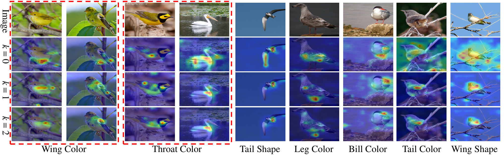
Consequently, by dynamically adjusting attribute prototypes according to the target image, PAL can progressively improve the attribute localization ability of visual representations, as shown in Fig. 3. PAL captures the attribute-region correspondence, which narrows the semantic-visual gap between category attributes and visual representations and boosts knowledge transfer between seen and unseen domains.

Besides exploring the correspondence between attributes and local image regions via PAL, we design a Progressive Category Classification (PCC) module to repel visual representations from different categories, which can enlarge category margins.

Similar to the sharing attribute prototypes in PAL, PCC defines a set of learnable category prototypes $\mathcal{C}^{0}=\{\boldsymbol{c}_{1}^{0},\cdots,\boldsymbol{c}_{N_{c}}^{0}\}$, where $\boldsymbol{c}_{j}^{0}\in\mathbb{R}^{N_{v}\times 1}$ records the visual representation center for the $j$-th category. $N_{c}=|\mathcal{Y}_{s}|$ is the number of seen categories. Since the attribute prototypes are progressively updated in PAL and $K$ visual representations $\{f^{k}(X)|k=1,\cdots,K\}$ are accordingly generated for each image, sharing category prototypes $\mathcal{C}^{0}$ cannot well model visual category differences for all iterations of $f^{k}(X)$. Thus, PCC is similarly designed to adjust category prototypes for different $f^{k}(X)$ by:

where $f_{cs}(\cdot)$ is a prototype selection function as shown in Fig. 2. Since $f^{k+1}(X)$ derives from $f^{k}(X)$, the category center at the $(k+1)$-th iteration should not deviate from that of the $k$-th iteration. Thus, $f_{cs}(\cdot)$ actually serves as a gating function implemented by channel attention mechanism, which controls the information flow from $\mathcal{C}^{k}$ to $\mathcal{C}^{k+1}$. This can ease the training difficulty of PCC by avoiding repetitive learning for $\mathcal{C}^{k+1}$. $W^{k}$ is a learnable bias at the $k$-th iteration, which supplements some specific information for $\mathcal{C}^{k+1}$.

At the $k$-th iteration, with the visual representation $f^{k}(X)$ and category prototypes $\mathcal{C}^{k}=\{\boldsymbol{c}_{1}^{k},\cdots,\boldsymbol{c}_{N_{c}}^{k}\}$, PCC repels different categories by:

Similar to $\mathcal{L}_{sa}^{k}$, $\mathcal{L}_{cl}^{k}$ is applied to all the $K$ iterations. Compared to $\mathcal{L}_{v2s}$ in Eq. \eqrefeq:basic_zsl, $\mathcal{L}_{cl}$ can better repel visual representations from different categories via progressive category prototypes $\{\mathcal{C}^{k}|k=1,\cdots,K\}$.

With progressively-updated category prototypes, PCC improves the category discriminability of visual representations $\{f^{k}(X)|k=1,\cdots,K\}$.

Overall, the objective loss function of DPPN is:

where $\lambda$ is the hyper-parameter to balance $\mathcal{L}_{cl}$. The attribute prototypes and category prototypes are collaboratively trained in a unified framework, which enables the final visual representation $f^{K}(X)$ to simultaneously capture attribute-region correspondence and category discrimination. During inference, only visual representation $f^{K}(X)$ at the $K$-th iteration is used by:

Compared to APN [47], DPPN is a much different and novel method with three main differences: a) instead of sharing prototypes for all images in APN, DPPN dynamically adjusts attribute prototypes according to different images. Specifically, DPPN introduces attribute-related clues from the target image feature into attribute prototypes, so that the prototypes are more adapted to the target image and result in better attribute localization; b) different from APN’s averagely pooling local visual features into a global one, DPPN concatenates local features to represent an image, which better preserves attribute-region correspondence. The final representation of DPPN is made up of attribute-localized features during both training and inference, instead of regarding attribute localization as mere supervision during training in APN; and c) DPPN further exploits progressive category prototypes to repel visual representations from different categories, which enhances category discrimination.

Datasets. Four public GZSL benchmarks, i.e., Caltech-USCD Birds-200-2011 (CUB) [43], SUN [35], Animals with Attributes2 (AWA2) [24], and Attribute Pascal and Yahoo (aPY) [14], are adopted in this paper. CUB contains $11,788$ bird images in $200$ species with $312$ description attributes. SUN contains $14,340$ scene images in $717$ classes with $102$ attributes. AWA2 contains $37,322$ animal images in $50$ classes with $85$ attributes. aPY contains $15,339$ object images in $32$ categories with $64$ attributes.

Evaluation Metrics. The widely-used harmonic mean $H=(2MCA_{u}\times MCA_{s})/(MCA_{u}+MCA_{s})$ is used to evaluate GZSL performance. $MCA_{s}$ and $MCA_{u}$ are the Mean Class Top-1 Accuracy for seen and unseen domains, respectively.

Implementation Details. The input images are resized to $448\times 448$ following [55, 45]. Random cropping and flipping are used for data augmentation. ResNet-101 [18] pretrained on ImageNet [12] is used as the backbone. A two-step training strategy is adopted, which trains DPPN with the fixed backbone and then fine-tunes the whole network on two 1080ti GPUs. Adam optimizer [22] is used with batch size of $64$ and $lr=2e-4$. $C=512$ since we use a conv. layer for dimension reduction after the backbone. $N_{a}$ is the number of attributes, which is $312$, $85$, $64$, $102$ for respective CUB, AWA2, aPY, and SUN. $K=3$ and $\lambda=1.0$. $N_{v}$ will be discussed in the ablation study.

Analysis of Attribute Localization and Category Discrimination. The core motivation of DPPN is to learn visual representations that simultaneously explore category discrimination and attribute-region correspondence via the proposed PCC and PAL, thus we analyse how PCC and PAL affect GZSL performance in this part. For simple comparison, we set $K=1$ in PCC and PAL. Results are listed in Table 1. "Base-V2S" is the baseline method trained by $\mathcal{L}_{v2s}$ in Eq. \eqrefeq:basic_zsl. "+PCC" adds PCC module to Base-V2S, which introduces stronger category discrimination constraint $\mathcal{L}_{cl}$. We can observe that "+PCC" obtains $1.1\%$ and $4.7\%$ gains on $H$ over "Base-V2S" on CUB and aPY. This is because that PCC explicitly pushes representations away from different categories via category prototypes, thus enlarging category margins for more accurate category classification and boosting GZSL. The third model "+PAL" replaces $f(\cdot)$ in "Base-V2S" with PAL, which enables visual representations with attribute localization ability. Compared with "Base-V2S", PAL module brings $4.9\%$ and $6.3\%$ gains on CUB and aPY. This derives from that PAL captures attribute-region correspondence by utilizing attribute prototypes to localize attribute-related local regions and produce attribute-specific visual representations. Finally, "+PCC&PAL" simultaneously considers category discrimination and attribute localization by incorporating both PCC and PAL, which obtains $7.1\%$ and $8.9\%$ gains. This proves that both attribute-region correspondence and category discrimination are critical to GZSL and complementary to each other.

Notably, PAL and PCC bring negligible additional computation, even when $K=3$, because $f_{rd}(\cdot)$ in Eq. \eqrefeq:final_vf controls the dimension of representation $f^{k}(X)$ to limit the computation burden. We visualize the difference of representation distribution between Base-V2S and our DPPN in the Appendix.

Effect of Progressive Prototype Updating. DPPN progressively updates attribute and category prototypes to learn more transferable and distinctive representations. Here, we analyse how such a progressive learning strategy impacts the attribute localization ability and category recognition by evaluating varying $K$ in PAL and PCC. The results are given in Fig. 4.

As $K$ rises from $1$ to $3$, $H$ on all the four datasets gradually increases. The best $H=73.5\%$, $73.1\%$, $48.4\%$, and $41.0\%$ on CUB, AWA2, aPY, and SUN is obtained when $K=3$. This demonstrates that, with category and attribute prototypes updated, the visual representations become more discriminative and transferable to the unseen categories. Here, to intuitively present the attribute localization progressively learned by PAL, we visualize the attribute localization results of PAL at different iteration $k$ when setting $K=3$. As shown in Fig. 3, the localization gets more and more precise as attribute prototypes gradually update. With progressively updated attribute prototypes, the PAL module can finally accurately localize corresponding attribute-related visual regions. Besides, with updating, the prototype for the same attribute gets more specific to the target image in the first four columns, reflecting that progressive updating can adapt prototypes according to different images. This proves that attribute prototypes can capture the attribute-region correspondence, and progressive updating makes prototypes more specific and distinctive. When $K>3$, $H$ drops. The reason may be that the over-updated prototypes become unstable and hard to train. $K=3$ is a good trade-off between general knowledge of a whole dataset and specific knowledge towards an image. Thus, we set $K=3$ for the rest experiments.

In summary, both quantitative and qualitative results demonstrate that progressive updating can improve attribute and category prototypes, which better captures attribute-region correspondence and category discrimination.

Evaluation of Components in PAL. PAL aims to learn visual representations with accurate attribute localization. Thus, we evaluate two important components of PAL, i.e., $f_{ar}(\cdot)$ in Eq. \eqrefeq:prograssive_assign and $cat(\cdot)$ in Eq. \eqrefeq:final_vf. The results are given in Table 2. $f_{ar}(\cdot)$ is a refinement function between $\mathcal{P}^{k}$ and $\mathcal{P}^{k+1}$ to improve prototype quality. As shown in the second row of Table 2, without $f_{ar}(\cdot)$, $H$ drops by $1.1\%$ and $2.9\%$ on CUB and aPY, respectively. This demonstrates that $f_{ar}(\cdot)$ benefits attribute prototype updating, thereby boosting attribute localization ability.

$cat(\cdot)$ is the aggregation function used to produce visual representation $f^{k}(X)$ by concatenating attribute prototypes $\mathcal{P}^{k}=\{\boldsymbol{p}_{1}^{k},\cdots,\boldsymbol{p}_{N_{a}}^{k}\}$. Compared to summing $\{\boldsymbol{p}_{1}^{k},\cdots,\boldsymbol{p}_{N_{a}}^{k}\}$ up or max pooling operation, $cat(\cdot)$ better preserves attribute-region correspondence. The third and fourth rows of Table 2 show that $H$ drops as replacing $cat(\cdot)$ with either summing up or max pooling. This proves that $cat(\cdot)$ benefits local correspondence preservation.

Effect of $f_{cs}(\cdot)$ in PCC. $f_{cs}(\cdot)$ in Eq. \eqrefeq:prograssive_C serves as a gating function to ease the training of category prototypes. In this part, we analyse the impact of $f_{cs}(\cdot)$. In Eq. \eqrefeq:prograssive_C, $f_{cs}(\cdot)$ removes redundancy in $\mathcal{C}^{k}$. Without $f_{cs}(\cdot)$, the category prototype updating becomes $\mathcal{C}^{k+1}=\mathcal{C}^{k}+W^{k+1}$, which passes all information in $\mathcal{C}^{k}$ to $\mathcal{C}^{k+1}$. The results are listed in the last row of Table 2. Without $f_{cs}(\cdot)$, $H$ drops by $1.6\%$ and $2.5\%$ on CUB and aPY. This proves that $f_{cs}(\cdot)$ helps to ease the training process of PCC, which learns more discriminative visual representations.

Effect of $\lambda$. $\lambda$ is the hyper-parameter to balance $\mathcal{L}_{cl}$. Here, we evaluate the effect of $\lambda$ as shown in Fig. 5 (a) and (b). As $\lambda$ rises from $0.0$ to $1.0$, i.e., category discrimination supervision $\mathcal{L}_{cl}$ is introduced into DPPN, $H$ increases on both CUB and aPY. The best $H$ is obtained when $\lambda=1.0$. This proves the effectiveness of category discrimination brought by PCC. When $\lambda>1.0$, $H$ starts to drop. Thus, we set $\lambda=1.0$ for better results.

Effect of $N_{v}$. $N_{v}$ is the dimension of $f^{k}(X)$ and $N_{v}=D\times N_{a}$. $N_{a}$ is the number of attributes, which are $312$, $85$, $64$, $102$ for CUB, AWA2, aPY, and SUN, respectively. Here, we set different $D$ to evaluate the effect of $N_{v}$ on recognition performance and calculation addition. Fig. 5 (c) shows the values of $H$ as $N_{v}$ varies. Fig. 5 (d) shows GLOPs addition over $N_{v}=512$. When $N_{v}$ is around $2,048$, best performance is obtained with a relatively small calculation complexity addition. Thus, we set $N_{v}=2496$, $2125$, $2048$, $2142$ and $D=8$, $25$, $32$, $21$ for CUB, AWA2, aPY, and SUN, respectively.

We compare DPPN with the state-of-the-art GZSL methods, of which the results are given in Table 3.

Among the existing methods, APN [47] is the most related method which also utilizes visual prototypes to localize visual parts. Different from APN that counts on only sharing prototypes for all images, our DPPN adjusts attribute prototypes dynamically according to the target image and exploits category prototypes to enhance category discrimination. Thus, DPPN learns specific and distinctive visual representations and surpasses APN by a large margin, i.e., $6.3\%$, $7.6\%$, and $3.4\%$ for $H$ on CUB, AWA2, and SUN datasets, respectively. APN does not provide codes and is approximately similar to PAL with $K=1$. As shown in Fig. 3, it qualitatively implies that progressive updating attribute prototypes can learn visual representations with better attribute localization ability. Besides, DAZLE [20] uses dense attribute attention to focus on relevant regions, which is inferior to DPPN by $15.4\%$, $6.0\%$, and $7.8\%$ on CUB, AWA2, and SUN, respectively. This proves the effectiveness of designing progressive attribute and category prototypes in GZSL.

Compared to other embedding-based methods, our method surpasses the best one by respectively $3.1\%$, $1.6\%$, and $9.4\%$ for $H$ on CUB, AWA2, aPY datasets, and obtains comparable best $H$ performance on SUN dataset. The results demonstrate that progressively exploring attribute-region correspondence and category discrimination can effectively enhance cross-domain transferability and category discriminability of visual representations. The reason for relatively small improvement on SUN may be that #categories is large while #images in each category is small in SUN, leading to difficulties for DPPN to learn accurate attribute localization and category discrimination.

Compared to generative methods that utilize additional unseen category labels during training, DPPN can achieve comparable, even better results, especially on CUB and AWA2 datasets. This reveals that with the assistance of progressive attribute localization and category discrimination, DPPN can surpass generative methods without complex GAN training.

References

- [1] Akata, Z., Perronnin, F., Harchaoui, Z., Schmid, C.: Label-embedding for image classification. IEEE Transactions on Pattern Analysis and Machine Intelligence 38(7), 1425–1438 (2016)
- [2] Akata, Z., Reed, S., Walter, D., Lee, H., Schiele, B.: Evaluation of output embeddings for fine-grained image classification. In: Proceedings of the IEEE Conference on Computer Vision and Pattern Recognition. pp. 2927–2936 (2015)
- [3] Annadani, Y., Biswas, S.: Preserving semantic relations for zero-shot learning. In: Proceedings of the IEEE Conference on Computer Vision and Pattern Recognition. pp. 7603–7612 (2018)
- [4] Atzmon, Y., Chechik, G.: Adaptive confidence smoothing for generalized zero-shot learning. In: Proceedings of the IEEE Conference on Computer Vision and Pattern Recognition. pp. 11671–11680 (2019)
- [5] Ba, J.L., Swersky, K., Fidler, S., salakhutdinov, R.: Predicting deep zero-shot convolutional neural networks using textual descriptions. In: Proceedings of the IEEE International Conference on Computer Vision. pp. 4247–4255 (2015)
- [6] Bucher, M., Herbin, S., Jurie, F.: Improving semantic embedding consistency by metric learning for zero-shot classiffication. In: Proceedings of the European Conference on Computer Vision. pp. 730–746 (2016)
- [7] Changpinyo, S., Chao, W.L., Gong, B., Sha, F.: Synthesized classifiers for zero-shot learning. In: Proceedings of the IEEE Conference on Computer Vision and Pattern Recognition. pp. 5327–5336 (2016)
- [8] Chao, W.L., Changpinyo, S., Gong, B., Sha, F.: An empirical study and analysis of generalized zero-shot learning for object recognition in the wild. In: Proceedings of the European Conference on Computer Vision. pp. 52–68 (2016)
- [9] Chen, L., Zhang, H., Xiao, J., Liu, W., Chang, S.F.: Zero-shot visual recognition using semantics-preserving adversarial embedding network. In: Proceedings of the IEEE Conference on Computer Vision and Pattern Recognition. pp. 1043–1052 (2018)
- [10] Chen, X., Lan, X., Sun, F., Zheng, N.: A boundary based out-of-distribution classifier for generalized zero-shot learning. In: Proceedings of the European Conference on Computer Vision. pp. 572–588 (2020)
- [11] Chou, Y.Y., Lin, H.T., Liu, T.L.: Adaptive and generative zero-shot learning. In: International Conference on Learning Representations (2021)
- [12] Deng, J., Dong, W., Socher, R., Li, L.J., Li, K., Fei-Fei, L.: Imagenet: A large-scale hierarchical image database. In: Proceedings of the IEEE Conference on Computer Vision and Pattern Recognition. pp. 248–255 (2009)
- [13] Ding, Z., Liu, H.: Marginalized latent semantic encoder for zero-shot learning. In: Proceedings of the IEEE Conference on Computer Vision and Pattern Recognition. pp. 6191–6199 (2019)
- [14] Farhadi, A., Endres, I., Hoiem, D., Forsyth, D.: Describing objects by their attributes. In: Proceedings of the IEEE Conference on Computer Vision and Pattern Recognition. pp. 1778–1785 (2009)
- [15] Ferrari, V., Zisserman, A.: Learning visual attributes. Advances in Neural Information Processing Systems 20, 433–440 (2007)
- [16] Frome, A., Corrado, G.S., Shlens, J., Bengio, S., Dean, J., Mikolov, T., et al.: Devise: A deep visual-semantic embedding model. In: Advances in Neural Information Processing Systems. pp. 2121–2129 (2013)
- [17] Han, Z., Fu, Z., Chen, S., Yang, J.: Contrastive embedding for generalized zero-shot learning. In: Proceedings of the IEEE Conference on Computer Vision and Pattern Recognition. pp. 2371–2381 (2021)
- [18] He, K., Zhang, X., Ren, S., Sun, J.: Deep residual learning for image recognition. In: Proceedings of the IEEE Conference on Computer Vision and Pattern Recognition. pp. 770–778 (2016)
- [19] Huang, H., Wang, C., Yu, P.S., Wang, C.D.: Generative dual adversarial network for generalized zero-shot learning. In: Proceedings of the IEEE Conference on Computer Vision and Pattern Recognition. pp. 801–810 (2019)
- [20] Huynh, D., Elhamifar, E.: Fine-grained generalized zero-shot learning via dense attribute-based attention. In: Proceedings of the IEEE Conference on Computer Vision and Pattern Recognition. pp. 4483–4493 (2020)
- [21] Jiang, H., Wang, R., Shan, S., Chen, X.: Transferable contrastive network for generalized zero-shot learning. In: Proceedings of the IEEE International Conference on Computer Vision. pp. 9765–9774 (2019)
- [22] Kingma, D.P., Ba, J.: Adam: A method for stochastic optimization. In: International Conference on Learning Representations (2015)
- [23] Kodirov, E., Xiang, T., Gong, S.: Semantic autoencoder for zero-shot learning. In: Proceedings of the IEEE Conference on Computer Vision and Pattern Recognition. pp. 3174–3183 (2017)
- [24] Lampert, C.H., Nickisch, H., Harmeling, S.: Learning to detect unseen object classes by between-class attribute transfer. In: Proceedings of the IEEE Conference on Computer Vision and Pattern Recognition. pp. 951–958 (2009)
- [25] Li, K., Min, M.R., Fu, Y.: Rethinking zero-shot learning: A conditional visual classification perspective. In: Proceedings of the IEEE International Conference on Computer Vision. pp. 3583–3592 (2019)
- [26] Li, Y., Wang, D., Hu, H., Lin, Y., Zhuang, Y.: Zero-shot recognition using dual visual-semantic mapping paths. In: Proceedings of the IEEE Conference on Computer Vision and Pattern Recognition. pp. 3279–3287 (2017)
- [27] Liu, L., Zhou, T., Long, G., Jiang, J., Dong, X., Zhang, C.: Isometric propagation network for generalized zero-shot learning. In: International Conference on Learning Representations (2021)
- [28] Liu, S., Long, M., Wang, J., Jordan, M.I.: Generalized zero-shot learning with deep calibration network. In: Advances in Neural Information Processing Systems. pp. 2005–2015 (2018)
- [29] Liu, Y., Guo, J., Cai, D., He, X.: Attribute attention for semantic disambiguation in zero-shot learning. In: Proceedings of the IEEE International Conference on Computer Vision. pp. 6698–6707 (2019)
- [30] Liu, Y., Zhou, L., Bai, X., Huang, Y., Gu, L., Zhou, J., Harada, T.: Goal-oriented gaze estimation for zero-shot learning. In: Proceedings of the IEEE Conference on Computer Vision and Pattern Recognition. pp. 3794–3803 (2021)
- [31] Min, S., Yao, H., Xie, H., Wang, C., Zha, Z.J., Zhang, Y.: Domain-aware visual bias eliminating for generalized zero-shot learning. In: Proceedings of the IEEE Conference on Computer Vision and Pattern Recognition. pp. 12664–12673 (2020)
- [32] Min, S., Yao, H., Xie, H., Zha, Z.J., Zhang, Y.: Domain-specific embedding network for zero-shot recognition. In: Proceedings of ACM International Conference on Multimedia. pp. 2070–2078 (2019)
- [33] Min, S., Yao, H., Xie, H., Zha, Z.J., Zhang, Y.: Domain-oriented semantic embedding for zero-shot learning. IEEE Transactions on Multimedia 23, 3919–3930 (2020)
- [34] Narayan, S., Gupta, A., Khan, F.S., Snoek, C.G., Shao, L.: Latent embedding feedback and discriminative features for zero-shot classification. In: Proceedings of the European Conference on Computer Vision. pp. 1–23 (2020)
- [35] Patterson, G., Hays, J.: Sun attribute database: Discovering, annotating, and recognizing scene attributes. In: Proceedings of the IEEE Conference on Computer Vision and Pattern Recognition. pp. 2751–2758 (2012)
- [36] Rahman, S., Khan, S., Porikli, F.: A unified approach for conventional zero-shot, generalized zero-shot, and few-shot learning. IEEE Transactions on Image Processing 27, 5652–5667 (2018)
- [37] Reed, S., Akata, Z., Lee, H., Schiele, B.: Learning deep representations of fine-grained visual descriptions. In: Proceedings of the IEEE Conference on Computer Vision and Pattern Recognition. pp. 49–58 (2016)
- [38] Romera-Paredes, B., Torr, P.: An embarrassingly simple approach to zero-shot learning. In: International Conference on Machine Learning. pp. 2152–2161 (2015)
- [39] Shen, Y., Qin, J., Huang, L.: Invertible zero-shot recognition flows. In: Proceedings of the European Conference on Computer Vision. pp. 614–631 (2020)
- [40] Shigeto, Y., Suzuki, I., Hara, K., Shimbo, M., Matsumoto, Y.: Ridge regression, hubness, and zero-shot learning. In: Joint European Conference on Machine Learning and Knowledge Discovery in Databases. pp. 135–151 (2015)
- [41] Socher, R., Ganjoo, M., Manning, C.D., Ng, A.: Zero-shot learning through cross-modal transfer. In: Advances in Neural Information Processing Systems. pp. 935–943 (2013)
- [42] Tong, B., Wang, C., Klinkigt, M., Kobayashi, Y., Nonaka, Y.: Hierarchical disentanglement of discriminative latent features for zero-shot learning. In: Proceedings of the IEEE Conference on Computer Vision and Pattern Recognition. pp. 11467–11476 (2019)
- [43] Wah, C., Branson, S., Welinder, P., Perona, P., Belongie, S.: The caltech-ucsd birds-200-2011 dataset. In: California Institute of Technology. pp. 1–8 (2011)
- [44] Xian, Y., Akata, Z., Sharma, G., Nguyen, Q., Hein, M., Schiele, B.: Latent embeddings for zero-shot classification. In: Proceedings of the IEEE Conference on Computer Vision and Pattern Recognition. pp. 69–77 (2016)
- [45] Xie, G.S., Liu, L., Jin, X., Zhu, F., Zhang, Z., Qin, J., Yao, Y., Shao, L.: Attentive region embedding network for zero-shot learning. In: Proceedings of the IEEE Conference on Computer Vision and Pattern Recognition. pp. 9384–9393 (2019)
- [46] Xie, G.S., Liu, L., Zhu, F., Zhao, F., Zhang, Z., Yao, Y., Qin, J., Shao, L.: Region graph embedding network for zero-shot learning. In: Proceedings of the European Conference on Computer Vision. pp. 562–580 (2020)
- [47] Xu, W., Xian, Y., Wang, J., Schiele, B., Akata, Z.: Attribute prototype network for zero-shot learning. In: Advances in Neural Information Processing Systems. pp. 21969–21980 (2020)
- [48] Ye, M., Guo, Y.: Progressive ensemble networks for zero-shot recognition. In: Proceedings of the IEEE Conference on Computer Vision and Pattern Recognition. pp. 11728–11736 (2019)
- [49] Yu, Y., Ji, Z., Fu, Y., Guo, J., Pang, Y., Zhang, Z.: Stacked semantic-guided attention model for fine-grained zero-shot learning. In: Advances in Neural Information Processing Systems. p. 5998–6007 (2018)
- [50] Yu, Y., Ji, Z., Han, J., Zhang, Z.: Episode-based prototype generating network for zero-shot learning. In: Proceedings of the IEEE Conference on Computer Vision and Pattern Recognition. pp. 14035–14044 (2020)
- [51] Yue, Z., Wang, T., Zhang, H., Sun, Q., Hua, X.S.: Counterfactual zero-shot and open-set visual recognition. In: Proceedings of the IEEE Conference on Computer Vision and Pattern Recognition. pp. 15404–15414 (2021)
- [52] Zhang, H., Long, Y., Guan, Y., Shao, L.: Triple verification network for generalized zero-shot learning. IEEE Transactions on Image Processing 28(1), 506–517 (2019)
- [53] Zhang, H., Koniusz, P.: Zero-shot kernel learning. In: Proceedings of the IEEE Conference on Computer Vision and Pattern Recognition. pp. 7670–7679 (2018)
- [54] Zhang, L., Xiang, T., Gong, S.: Learning a deep embedding model for zero-shot learning. In: Proceedings of the IEEE Conference on Computer Vision and Pattern Recognition. pp. 2021–2030 (2017)
- [55] Zhu, P., Wang, H., Saligrama, V.: Generalized zero-shot recognition based on visually semantic embedding. In: Proceedings of the IEEE Conference on Computer Vision and Pattern Recognition. pp. 2995–3003 (2019)