Production and transport of vorticity in two-dimensional Rayleigh-Bénard convection cellPreprint: Preprint submit to Physics of Fluids
Abstract
We present a numerical study of vorticity production and transport in the two-dimensional Rayleigh-Bénard (RB) convection. Direct numerical simulations are carried out in the Rayleigh number () range , the Prandtl number () of 0.71, and the aspect ratio () of the convection cell range . We found that the flow structure and temperature distribution vary with greatly due to multiple vortices interaction. Further investigation on the vorticity production and transport reveals that, in the RB convection, in addition to the vorticity production due to wall shear stress, buoyancy produces significant vorticity in the bulk region. The produced vorticity is transported via advection and diffusion. An interesting finding is that the main vortices and the corner vortices can be visualized via the contour of buoyancy-produced vorticity. Although a vigorous definition of the vortex is still lacking in the community, our efficient vortex visualization approach in the RB convection may shed light on further research toward vortex identification. We also found that the spatial distribution of vorticity flux along the wall is positively correlated with that of the Nusselt number (), suggesting the amount of vorticity that enters the flow is directly related to the amount of thermal energy that enters the flow. 11 1 This article may be downloaded for personal use only. Any other use requires prior permission of the author and AIP Publishing. This article appeared in Xu et al., Phys. Fluids 34, 013609 (2022) and may be found at https://doi.org/10.1063/5.0072873.
I Introduction
Thermal convection occurs ubiquitously in nature and has wide applications in industry, such as convection over the city, Omidvar et al. 2020 convection in the indoor environment, Bhagat et al. 2020; Xu et al. 2020a convection in the heat exchanger reactor, Shah and Sekulic 2003 and so on. A canonic flow systems for studying thermal convection is Rayleigh-Bénard (RB) convection, Lohse and Xia 2010; Xia 2013 in which the fluid is heated from the bottom wall and cooled from the top wall. In thermal convection cells, approaches to enhance heat transfer efficiency include creating roughness on the heating walls, Zhang et al. 2018; Dong et al. 2020 geometrical confinement of the convection cell, Huang et al. 2013; Huang and Xia 2016 vibration-induced boundary-layer destabilization, Wang, Zhou, and Sun 2020; Wu et al. 2021 and many others.
Previous studies have revealed the connections between heat transfer efficiency (in terms of dimensionless Nusselt number, ) and flow structures. Sun, Xi, and Xia 2005; Xi and Xia 2008; Xi et al. 2016; Xu et al. 2020b; van der Poel, Stevens, and Lohse 2011; van der Poel et al. 2012; Zou et al. 2019; Zhu and Zhou 2021 For example, Sun et al. Sun, Xi, and Xia 2005 measured the in both leveled and tilted cylindrical cells, in which the large-scale circulation is either azimuthal or locked in a particular orientation, respectively. They found that the is larger in the leveled cell than that in the tilted one, thus demonstrating that different flow structures can give rise to different values of . Xi et al. Xi and Xia 2008 further observed that both the single-roll and the double-roll flow structures exist in the large-scale flow. They examined the averaged corresponding to a particular flow structure, and they found that the single-roll flow structure is more efficient for heat transfer than the double-roll structure. Later, Xi et al. Xi et al. 2016 found that has a momentary overshoot above its average value during flow reversal event, which is also numerically verified by Xu et al. Xu et al. 2020b The overshoot in was attributed to more coherent flow or plumes for the short period of time during reversal. van der Poel et al. van der Poel, Stevens, and Lohse 2011; van der Poel et al. 2012 simulated the aspect ratio dependence of heat transfer efficiency in a two-dimensional (2D) square cell. They conditionally averaged based on flow structures, and they found that heat transfer is more efficient with less vertically arranged vortex or less horizontally elongated vortex. Xu et al. Xu et al. 2020b adopted the Fourier mode decomposition and the proper orthogonal decomposition to extract the coherent flow structure. They showed that the single-roll mode, the horizontally stacked double-roll mode, and the quadrupolar flow mode are more efficient for heat transfer on average; in contrast, the vertically stacked double-roll mode is inefficient for heat transfer on average. Xu et al. 2020b
On the other hand, it is advantageous to interpret the fluid flows in terms of vorticity, which is defined as the curl of velocity . Panton 2013; Davidson 2015 The vorticity represents the rotation of a fluid particle, and only the shear stresses can rotate the fluid particle. As for the pressure and the normal viscous stresses, they act through the center of the fluid particle and cannot rotate fluid particles. Thus, analyzing vorticity dynamics will reveal physical mechanisms for fluid flows and associate transport processes (e.g., heat transfer, mass transfer, ion transfer) that may be hidden from the velocity and pressure fields. In the industry, various vortex generators have been designed to enhance transfer in heat exchanger reactors; Lemenand et al. 2018; Karkaba et al. 2020 however, most of those studies focused on a global relationship between the velocity field and heat transfer efficiency, and the role of vorticity transport in heat transfer enhancement remains unclear.
In this work, we will provide a comprehensive analysis of vorticity production and transport in the simple yet canonic RB convection. Our motivation is to reveal the connections between heat transfer efficiency and the vorticity field. The rest of the paper is organized as follows. In Sec. II, we will present the numerical method for simulating incompressible thermal convection. The in-house numerical solver based on the lattice Boltzmann (LB) method will be introduced. In Sec. III, we will first provide general flow and heat transfer features in the convection cells; after that, we will analyze vorticity production due to wall shear stress and buoyancy, as well as vorticity transport due to advection and diffusion. In Sec. IV, the main findings of the present work are summarized.
II Numerical method
II.1 Mathematical model for thermal convection
We consider incompressible thermal flows under the Boussinesq approximation. The temperature is treated as an active scalar and its influence on the velocity field is realized through the buoyancy term. The viscous heat dissipation and compression work are neglected, and all the transport coefficients are assumed to be constants. Then, the governing equations can be written as
| (1a) | ||||
| (1b) | ||||
| (1c) | ||||
where , , and are velocity, pressure, and temperature of the fluid, respectively. , , and are the reference pressure, density and temperature, respectively. , , and are the thermal expansion coefficient, kinematic viscosity, and thermal diffusivity, respectively. is the gravity acceleration value. is the unit vector parallel to the gravity. With the following non-dimensional group
| (2) |
Then, Eq. (1) can be rewritten in dimensionless form as
| (3a) | ||||
| (3b) | ||||
| (3c) | ||||
Here, is the cell height and is the temperature difference between heating and cooling walls. is the reference pressure. In this paper, unless otherwise stated, the dimensionless variable is denoted with a superscript star. The two dimensionless parameters are the Rayleigh number () and the Prandtl number (), which are defined as
| (4) |
II.2 The lattice Boltzmann method for incompressible thermal flows
The LB method to solve fluid flows and heat transfer is based on the double distribution function approach. The advantages of the LB method include easy implementation and parallelization as well as low numerical dissipation. Chen and Doolen 1998; Aidun and Clausen 2010; Xu, Shyy, and Zhao 2017 Specifically, we chose a D2Q9 model for the Navier-Stokes equations to simulate fluid flows and a D2Q5 model for the energy equation to simulate heat transfer. To enhance the numerical stability, the multi-relaxation-time collision operator is adopted in the evolution equations of both density and temperature distribution functions. The evolution equation of the density distribution function is written as
| (5) |
where is the density distribution function. is the fluid parcel position, is the time, and is the time step. is the discrete velocity along the th direction. is a orthogonal transformation matrix that projects the density distribution function and its equilibrium from the velocity space onto the moment space, such that and . is the diagonal relaxation matrix. The macroscopic density and velocity are obtained from the density distribution function as
| (6) |
The evolution equation of temperature distribution function is written as
| (7) |
where is the temperature distribution function. is a orthogonal transformation matrix that projects the temperature distribution function and its equilibrium from the velocity space onto the moment space, such that and . is the diagonal relaxation matrix. The macroscopic temperature is obtained from the temperature distribution function as
| (8) |
Our in-house LB solver is accelerated with OpenACC directives to utilize the computing power of GPUs. Xu, Shi, and Zhao 2017 More numerical details of the LB method and validation of the in-house solver can be found in our previous work. Xu, Shi, and Xi 2019a; Xu, Shi, and Xi 2019b; Xu, Chen, and Xi 2021
II.3 Simulation settings
The top and bottom walls of the convection cell are kept at constant cold and hot temperature, respectively, while the other two vertical walls are adiabatic. All four walls impose no-slip velocity boundary conditions. The dimension of the cell is . Here, is the cell length. Simulation results are provided for the in the range , the of 0.71, and cell aspect ratio () in the range . The criterion for reaching a steady state is
| (9) |
For unsteady flows, after the flows reach the statistically stationary state, we take average time of to obtain statistically convergent results. The time-averaged value of variable is define as , where is the time duration of the flow in the fully developed state.
We first refine the grid to check the convergence behaviors of the in-house LB solvers. We calculated response parameters including the Nusselt number () and the Reynolds number (), which describe the heat transfer efficiency and flow strength, respectively,
| (10) |
Here, denotes the spatial and temporal average. In Table 1, we list the steady solution of , , and the absolute value of vorticity at cell center () obtained at , , and . From Table 1, we can see that results calculated from the LB solver monotonous converge.
| Grid | |||
|---|---|---|---|
| 6.4393 | 274.40 | 1.5280 | |
| 6.3489 | 275.36 | 1.5114 | |
| 6.3336 | 275.62 | 1.5074 | |
| 6.3299 | 275.70 | 1.5066 | |
| 6.3290 | 275.72 | 1.5064 | |
| 6.3287 | 275.72 | 1.5064 | |
| 6.3287 | 275.72 | 1.5064 |
To quantitatively evaluate the spatial convergence order, we assume the results obtained at the largest grid of are accurate and calculate the error as . Here, denotes flow variables calculated with a mesh size of . From Fig. 1, we can see that the LB solver is second-order spatial accuracy for simulating velocity and temperature fields. In addition, the vorticity field, which is obtained from the curl of velocity field data using a third-order finite difference scheme, also exhibits second-order spatial accuracy. It should be noted that numerics in Table 1 are presented with five significant numbers for clarity of writing; while the data in Fig. 1 are calculated with eight significant numbers. The mesh independent tests indicate that a grid resolution of 256 is adequate for the simulation. Thus, we use at least 256 grids to resolve the cell length or the cell height. Other detailed simulation parameters are listed in Table 2. In addition, we list the response parameters of and in Table 2. At fixed and , with the increase in , both the and gradually increase to an asymptotic value.

| Grid | Flow state | ||||||
|---|---|---|---|---|---|---|---|
| 0.71 | 0.75 | Unsteady | 1000 | 2.44 | 49.47 | ||
| 0.71 | 1 | Steady | - | 3.92 | 84.43 | ||
| 0.71 | 2 | Steady | - | 4.43 | 100.97 | ||
| 0.71 | 4 | Steady | - | 4.75 | 109.29 | ||
| 0.71 | 6 | Steady | - | 4.84 | 111.58 | ||
| 0.71 | 0.75 | Steady | - | 3.34 | 99.93 | ||
| 0.71 | 1 | Steady | - | 5.03 | 151.57 | ||
| 0.71 | 2 | Steady | - | 5.73 | 182.68 | ||
| 0.71 | 4 | Steady | - | 6.22 | 199.36 | ||
| 0.71 | 6 | Steady | - | 6.37 | 203.89 | ||
| 0.71 | 0.75 | Steady | - | 4.62 | 202.33 | ||
| 0.71 | 1 | Steady | - | 6.33 | 275.70 | ||
| 0.71 | 2 | Steady | - | 7.39 | 340.87 | ||
| 0.71 | 4 | Steady | - | 8.25 | 377.48 | ||
| 0.71 | 6 | Unsteady | 1000 | 8.47 | 386.54 |
III Results and discussion
III.1 General flow and heat transfer features
We first present general flow and heat transfer patterns in the convection cell. Figure 2 shows the contour of velocity magnitude, temperature field, and pressure field in the RB convection at , , and . Here, the reference temperature is chosen as the temperature of the cold wall, that is, such that the dimensionless temperature varies between zero and one. The reference pressure is chosen as the pressure at the cell center, that is, such that the dimensionless pressure at the cell center equals zero. In the RB convection, velocity magnitude exhibits large values near all four walls. In the bulk region of the RB convection, the clockwise rotated large-scale vortex exhibits a circular shape; near the top-left and bottom-right corners, there exist two counterclockwise rotated small vortices [see Fig. 2(a)]. Thin thermal boundary layers appear near the bottom and top horizontal walls [see Fig. 2(b)], where the fluids are heating and cooling, respectively. Driven by the clockwise large-scale circulation, detached hot plumes arise along the left adiabatic wall, and cold plumes fall along the right adiabatic wall. From the pressure field [see Fig. 2(c)], we observe a strong gradient of pressure along the vertical direction, while the pressure contour is slightly twisted along the horizontal direction. It should be noted that the pressure shown here (and the corresponding dimensionless one) is based on the Boussinesq approximation, and it is related to the hydrodynamic pressure via the relation of . For the dimensionless pressure under the Boussinesq approximation , we can rewrite it as , which indicates there is an additional term compared to that in the dimensionless hydrodynamic pressure .

In the above, we discussed flow and heat transfer patterns in the convection cell of a unit square, that is, cell aspect ratio . Next, we focus on rectangular cells with and , respectively. In Fig. 3, we show flow and heat transfer patterns in the RB convection with . We can observe two horizontally stacked main vortices in the cell [see Fig. 3(a)]. These two counter-rotating vortices carry hot rising plumes along the vertical left and right walls. At the top wall, the fluids are cooling down, cold plumes emerge and they fall along the vertical mid-plane of the cell, and the temperature field preserves left-right symmetry, as shown in Fig. 3(b). The contour of the pressure field in the RB convection [see Fig. 3(c)] is also twisted along the horizontal direction, and the trend is more obvious where the falling cold plumes eject on the hot bottom walls.

Figure 4 further presents flow and heat transfer patterns in the RB convection with . We observe two vertically stacked main vortices in the cell [see Fig. 4(a)]. The velocity magnitude reaches its maximum at the horizontal mid-plane, where the two main vortices interact. The bottom counterclockwise rotated vortex carries hot rising plumes, while the top clockwise rotated vortex carries cold falling plumes [see Fig. 4(b)]. The plumes exchange thermal energy at the horizontal mid-plane, and the temperature field preserves the top-bottom symmetry. In addition, the contour of the pressure field along the horizontal direction in the cell [see Fig. 4(c)] is less twisted than that in the cell [see Fig. 3(c)].

III.2 Vorticity production due to wall shear stress
To describe how much vorticity is entering the flow from the wall, we used the metrics of vorticity flux . Here, is the plane orientation. In two dimensions, we only have non-zero components of vorticity as . Thus, the vorticity flux along the vertical walls (i.e., ) is , and the vorticity flux along the horizontal walls (i.e., ) is . On the other hand, the heat flux perpendicular to the wall is , and we normalize the heat flux with that due to pure conduction , and then, we can use the dimensionless Nusselt number at the wall to describe how much thermal energy is entering the flow. Here, denotes the thermal conductivity of the fluid. In Fig. 5, we plot the distribution of dimensionless vorticity flux and the normalized Nusselt number along top and bottom walls. Here, denotes the maximum value of along all four walls. In the cell [see Figs. 5(a) and 5(b)], the spatial distribution of the profile and the profile is antisymmetric along the top and bottom walls. Along the horizontal walls, we can observe one peak and one valley near the central part of the wall. Here, the negative values of imply the vorticity that enters the flow is clockwise rotating. Both the positive and negative neighboring vorticity lead to enhanced thermal energy that enters the flow, and thus, we can observe a peak in the .

In the cell [see Figs. 5(c) and 5(d)], along the top (or the bottom) wall, the minimum values of correspond to the positions where cold (or hot) plumes are released, and the maximum values of correspond to the positions where hot (or cold) plumes are imping and penetrating the wall. Previously, Kenjereš and Hanjalić Kenjereš and Hanjalić 2000 reported the asymmetric of the profile along the top and bottom walls in the cell. Here, we found that the profile along the top and bottom walls is also asymmetric. More importantly, we found the spatial distribution of along the heating and cooling walls can be well explained by the spatial distribution of . In the profile, a peak and a valley imply vorticity with opposite rotating direction is entering the flow; correspondingly, we can then observe a peak in the profile. The reason is that the amount of vorticity (regardless of the rotating direction) that enters the flow is directly related to the amount of thermal energy that enters the flow. In Fig. 5(c), along the top wall, there are two pairs of peak and valley in the vorticity flux profile, and thus, there are two peaks in the profile. In Fig. 5(d), along the bottom wall, there is one peak and one valley in the vorticity flux profile, and thus, there is only one peak in the profile. In the cell [see Figs. 5(e) and 5(f)], the two large-scale vortices are vertically stacked, and there is only one peak and valley in the profile along the horizontal walls, which is similar to that in the cell. Correspondingly, the profile shows a peak where extreme values of appear. Thus, we can analyze the spatial distribution of along the heating and cooling walls via the vorticity flux along the wall.
Although vorticity can be viewed as the signatures of fluid motion, it is the pressure gradients that drive the flow. In the vorticity transport equation, the pressure does not appear; thus, it does not directly change the vorticity. It should be noted that the buoyancy appears in the momentum equation as an external body force, and thus, the effective pressure gradients are a combination of original pressure gradients and buoyancy. In Fig. 6, we show the dimensionless effective pressure gradients (i.e., and ) in the RB convection. We are particularly interested in the pressure gradients along the wall, which is necessary to sustain a flux of vorticity into the fluid. Because the velocity is zero at the wall, from the momentum equation, we have . Comparing Fig. 5 with Fig. 6, we can verify that positive along the bottom (or top) wall is indeed caused by the positive (or negative) value of horizontal effective pressure gradient.
To quantitatively describe the vorticity flux as functions of the flow control parameters, we calculate the average of along the horizontal top and bottom walls. Because positive and negative values of simply imply the vorticity that enters the flow with opposite rotating direction, we take the absolute values of to do the average, namely, . Figure 7 (a) shows the aspect ratio dependence of average vorticity flux at , , and . We can see that with the increase in , the average vorticity flux along the horizontal walls and monotonously increases and gradually approach an asymptotic value. We then normalize with , and all data fall on top of each other and the shape of do not change with , as shown in Fig. 7 (b). The results shown here thus suggest universal properties of vorticity flux along the heating and cooling walls with respect to different .

III.3 Vorticity production due to buoyancy
The vorticity transport equation for incompressible thermal convection can be obtained by taking the curl of the momentum equation, which is written as Wu, Ma, and Zhou 2007
| (11) |
In two dimensions, the velocity vector is , and thus, we only have non-zero components of vorticity as . There is no vortex stretching nor tilting ( is always zero), and thus, vorticity production does not come from shearing effects in two dimensions. In addition, the body force (i.e., buoyancy) is ; then, the above vorticity transport equation can be rewritten as
| (12) |
With the non-dimensional group in Eq. (2), the dimensionless vorticity transport equation for incompressible thermal flows is written as
| (13) |
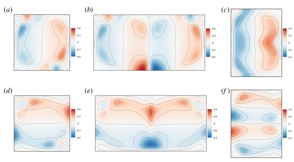
In Fig. 8, we further provide the contour of vorticity produced by buoyancy, namely, the contour of . An interesting finding is that the position of buoyancy-produced vorticity accumulates exactly where the vortices lay. Specifically, in the cell [see Fig. 8(a)], counterclockwise rotated buoyancy-produced vorticity accumulates near the left-top and right-bottom corner of the cell, where counterclockwise rotated corner vortices exist [compared to Fig. 2(a)]. In addition, clockwise rotated buoyancy-produced vorticity accumulates and forms the edge of the main clockwise rotating vortex. Thus, in Fig. 8, the red color region represents counterclockwise rotating vortices, and the blue color region represents the clockwise rotating vortices. We can also observe similar patterns in the and the cell. We propose to use the contour of buoyancy-produced vorticity, that is, , as a metric to visualize the vortex in the RB convection. It should be mentioned that at present, this approach is only valid for two-dimensional flow, and extension to three-dimensional flows deserves future investigation.

We also check the amount of vorticity, without regard to direction, which is measured by enstrophy . The enstrophy transport equation can be obtained via the inner production of with Eq. (11), which is written as Wu, Ma, and Zhou 2007
| (14) |
Here, denotes the strain rate tensor. In two dimensions, the term is always zero. With the non-dimensional group in Eq. (2), the dimensionless enstrophy transport equation for incompressible thermal flows in two dimensions is written as
| (15) |
In Fig. 9, we provide the contour of enstrophy produced by buoyancy. We can see that due to buoyancy, intense enstrophy production (or destruction) occurs at the inner (or outer) edge of the main vortices; intense enstrophy production also occurs at regions of corner vortices. Analysis of spatial distribution of buoyancy-produced vorticity and buoyancy-produced enstrophy indicate that buoyancy significantly affects the flow structure in the Rayleigh-Bénard convection, and contour of buoyancy-produced vorticity and buoyancy-produced enstrophy can be used to visualize the vortices in the two-dimensional Rayleigh-Bénard convection.

It should be noted that the precise definition of a vortex is still an open question. Previously, various criteria to identify a vortex have been proposed. Hunt, Wray, and Moin 1988; Jeong and Hussain 1995; Chong, Perry, and Cantwell 1990; Zhou et al. 1999 In Fig. 10, we show the vortex identification using the Q-criterion, Hunt, Wray, and Moin 1988 the -criterion, Jeong and Hussain 1995 the -criterion, Chong, Perry, and Cantwell 1990 and the swirling-strength criterion Zhou et al. 1999 in the RB convection. Although those methods can be used to identify the vortices region, they failed to indicate the rotating direction of the vortices. Our method can be used to identify the vortices regions as well as the rotating direction of the vortices, which serves as an efficient vortex visualization approach. Overall, our analysis of the vorticity distribution provides an alternative understanding of the flow structure in the thermal convection cells.

III.4 Vorticity transport due to advection and diffusion
The vorticity redistribution mechanism is mainly due to advection and diffusion transport. In Fig. 11(a), we show the contour of the vorticity component in the cell. We can observe strong positive values of (i.e., counterclockwise rotated vorticity) mainly appear near the walls, and it is near zero in the bulk region of the cell. This can be simply understood as the velocity gradients are large near the wall, as evident from the clockwise rotated large-scale circulation "wind" in the cell [see Fig. 2(a)]. A fluid particle near the left bottom (or the right top) wall will first feel the influence of the large-scale circulation and gain some vorticity. After some time, it will move up (or down) along the vertical walls and diffuse out from the wall; thus, the thickness of the diffusion layer for vorticity near the left (or the right) wall will grow from the bottom (or top) to top (or bottom). In Fig. 11(b), we further show advection of vorticity and we can see that two pairs of counter-rotating vorticity coexist along each of the four walls. Near the wall, the advection of vorticity [see Fig. 11(b)] is strongly influenced by the redistribution of wall-produced vorticity. Taking the top wall as an example, at around , negative values of vorticity are entering the fluid [as evident by the valley in vorticity flux profile shown in Fig. 5(a), see more discussion in Sec. III.2], which corresponds to the advection of clockwise rotated vorticity [i.e., a negative value in the contour of Fig. 11(b)]. On the contrary, at around , positive values of vorticity are entering the fluid [as evident by the peak in vorticity flux profile shown in Fig. 5(a)], which corresponds to the advection of counterclockwise rotated vorticity [i.e., positive value in the contour of Fig. 11(b)]. Similarly, we can analyze the distribution of vorticity advection near the other three walls. As for the diffusion of vorticity due to the viscous effect, the pattern of vorticity diffusion is similar to that of vorticity advection [see Fig. 11(c)], and the main differences are caused by the production of either counterclockwise or clockwise rotated vorticity due to buoyancy. Meanwhile, from Fig. 11, we can see that in the cell, the redistribution of vorticity advection and vorticity diffusion preserves top-bottom antisymmetric property. In the RB convection with or , the aspect ratio does not significantly influence the vorticity transport. For the sake of clarity, we will not repeat the detailed discussion here, but only show the contour plot in the Appendix.

IV Conclusions
In this work, we analyzed the vorticity production and transport in the RB convection. Specifically, with flow field and temperature field information (via solving fluid flows and heat transfer equations), we calculated each term in the vorticity transport equation. We examined the vorticity advection, diffusion, and production due to buoyancy and wall shear stress. The main findings are summarized as follows:
- 1.
The flow structure and temperature distribution vary with greatly due to multiple vortices interaction. In addition to vorticity redistribution, buoyancy produces significant vorticity in the bulk region, resulting in a richer vortices structure.
- 2.
The main vortices and the corner vortices can be visualized via the contour of buoyancy-produced vorticity. This method can be used to identify the vortices regions as well as the rotating direction of the vortices, which serves as an efficient vortex visualization approach.
- 3.
The spatial distribution of vorticity flux along the heating and cooling walls is positively correlated with that of , suggesting the amount of vorticity that enters the flow is directly related to the amount of thermal energy that enters the flow.
Acknowledgements.
This work was supported by the National Natural Science Foundation of China (NSFC) through Grant Nos. 11902268 and 11772259, the National Key Project No. GJXM92579, the Fundamental Research Funds for the Central Universities of China (No. D5000200570), and the 111 project of China (No. B17037).AUTHOR DECLARATIONS
Conflict of Interest
The authors declare no competing interests.
Data Availability
The data that support the findings of this study are available from the corresponding author upon reasonable request.
Appendix: Vorticity transport in cell and cell
In the RB convection with , the clockwise (or counterclockwise) rotated main vortex sitting in the left-half (or right-half) of the cell induce counterclockwise (or clockwise) rotated vorticity near the horizontal walls (see Fig. 12). In the RB convection with , the clockwise (or counterclockwise) rotated main vortex sitting in the top-half (or bottom-half) of the cell induce counterclockwise (or clockwise) rotated vorticity near the vertical walls (see Fig. 13). As for the differences among vorticity, vorticity advection, and vorticity diffusion, one may refer to the previous discussion in the cell.


References
- Omidvar et al. (2020) H. Omidvar, E. Bou-Zeid, Q. Li, J.-P. Mellado, and P. Klein, “Plume or bubble? Mixed-convection flow regimes and city-scale circulations,” Journal of Fluid Mechanics 897, A5 (2020).
- Bhagat et al. (2020) R. K. Bhagat, M. D. Wykes, S. B. Dalziel, and P. Linden, “Effects of ventilation on the indoor spread of COVID-19,” Journal of Fluid Mechanics 903, F1 (2020).
- Xu et al. (2020a) A. Xu, S. Tao, L. Shi, and H.-D. Xi, “Transport and deposition of dilute microparticles in turbulent thermal convection,” Physics of Fluids 32, 083301 (2020a).
- Shah and Sekulic (2003) R. K. Shah and D. P. Sekulic, Fundamentals of heat exchanger design (John Wiley & Sons, 2003).
- Lohse and Xia (2010) D. Lohse and K.-Q. Xia, “Small-scale properties of turbulent Rayleigh-Bénard convection,” Annual Review of Fluid Mechanics 42, 335–364 (2010).
- Xia (2013) K.-Q. Xia, “Current trends and future directions in turbulent thermal convection,” Theoretical and Applied Mechanics Letters 3, 052001 (2013).
- Zhang et al. (2018) Y.-Z. Zhang, C. Sun, Y. Bao, and Q. Zhou, “How surface roughness reduces heat transport for small roughness heights in turbulent Rayleigh–Bénard convection,” Journal of Fluid Mechanics 836, R2 (2018).
- Dong et al. (2020) D.-L. Dong, B.-F. Wang, Y.-H. Dong, Y.-X. Huang, N. Jiang, Y.-L. Liu, Z.-M. Lu, X. Qiu, Z.-Q. Tang, and Q. Zhou, “Influence of spatial arrangements of roughness elements on turbulent Rayleigh-Bénard convection,” Physics of Fluids 32, 045114 (2020).
- Huang et al. (2013) S.-D. Huang, M. Kaczorowski, R. Ni, and K.-Q. Xia, “Confinement-induced heat-transport enhancement in turbulent thermal convection,” Physical Review Letters 111, 104501 (2013).
- Huang and Xia (2016) S.-D. Huang and K.-Q. Xia, “Effects of geometric confinement in quasi-2-D turbulent Rayleigh–Bénard convection,” Journal of Fluid Mechanics 794, 639–654 (2016).
- Wang, Zhou, and Sun (2020) B.-F. Wang, Q. Zhou, and C. Sun, “Vibration-induced boundary-layer destabilization achieves massive heat-transport enhancement,” Science Advances 6, eaaz8239 (2020).
- Wu et al. (2021) J.-Z. Wu, Y.-H. Dong, B.-F. Wang, and Q. Zhou, “Phase decomposition analysis on oscillatory Rayleigh–Bénard turbulence,” Physics of Fluids 33, 045108 (2021).
- Sun, Xi, and Xia (2005) C. Sun, H.-D. Xi, and K.-Q. Xia, “Azimuthal symmetry, flow dynamics, and heat transport in turbulent thermal convection in a cylinder with an aspect ratio of 0.5,” Physical Review Letters 95, 074502 (2005).
- Xi and Xia (2008) H.-D. Xi and K.-Q. Xia, “Flow mode transitions in turbulent thermal convection,” Physics of Fluids 20, 055104 (2008).
- Xi et al. (2016) H.-D. Xi, Y.-B. Zhang, J.-T. Hao, and K.-Q. Xia, “Higher-order flow modes in turbulent Rayleigh–Bénard convection,” Journal of Fluid Mechanics 805, 31–51 (2016).
- Xu et al. (2020b) A. Xu, X. Chen, F. Wang, and H.-D. Xi, “Correlation of internal flow structure with heat transfer efficiency in turbulent Rayleigh–Bénard convection,” Physics of Fluids 32, 105112 (2020b).
- van der Poel, Stevens, and Lohse (2011) E. P. van der Poel, R. J. Stevens, and D. Lohse, “Connecting flow structures and heat flux in turbulent Rayleigh-Bénard convection,” Physical Review E 84, 045303 (2011).
- van der Poel et al. (2012) E. P. van der Poel, R. J. Stevens, K. Sugiyama, and D. Lohse, “Flow states in two-dimensional Rayleigh-Bénard convection as a function of aspect-ratio and Rayleigh number,” Physics of Fluids 24, 085104 (2012).
- Zou et al. (2019) H.-Y. Zou, W.-F. Zhou, X. Chen, Y. Bao, J. Chen, and Z.-S. She, “Boundary layer structure in turbulent Rayleigh–Bénard convection in a slim box,” Acta Mechanica Sinica 35, 713–728 (2019).
- Zhu and Zhou (2021) X. Zhu and Q. Zhou, “Flow structures of turbulent Rayleigh–Bénard convection in annular cells with aspect ratio one and larger,” Acta Mechanica Sinica 37, 1291–1298 (2021).
- Panton (2013) R. L. Panton, Incompressible flow (John Wiley & Sons, 2013).
- Davidson (2015) P. A. Davidson, Turbulence: An introduction for scientists and engineers (Oxford university press, 2015).
- Lemenand et al. (2018) T. Lemenand, C. Habchi, D. Della Valle, and H. Peerhossaini, “Vorticity and convective heat transfer downstream of a vortex generator,” International Journal of Thermal Sciences 125, 342–349 (2018).
- Karkaba et al. (2020) H. Karkaba, T. Dbouk, C. Habchi, S. Russeil, T. Lemenand, and D. Bougeard, “Multi objective optimization of vortex generators for heat transfer enhancement using large design space exploration,” Chemical Engineering and Processing-Process Intensification 154, 107982 (2020).
- Chen and Doolen (1998) S. Chen and G. D. Doolen, “Lattice Boltzmann method for fluid flows,” Annual Review of Fluid Mechanics 30, 329–364 (1998).
- Aidun and Clausen (2010) C. K. Aidun and J. R. Clausen, “Lattice-Boltzmann method for complex flows,” Annual Review of Fluid Mechanics 42, 439–472 (2010).
- Xu, Shyy, and Zhao (2017) A. Xu, W. Shyy, and T. Zhao, “Lattice Boltzmann modeling of transport phenomena in fuel cells and flow batteries,” Acta Mechanica Sinica 33, 555–574 (2017).
- Xu, Shi, and Zhao (2017) A. Xu, L. Shi, and T. Zhao, “Accelerated lattice Boltzmann simulation using GPU and OpenACC with data management,” International Journal of Heat and Mass Transfer 109, 577–588 (2017).
- Xu, Shi, and Xi (2019a) A. Xu, L. Shi, and H.-D. Xi, “Lattice Boltzmann simulations of three-dimensional thermal convective flows at high Rayleigh number,” International Journal of Heat and Mass Transfer 140, 359–370 (2019a).
- Xu, Shi, and Xi (2019b) A. Xu, L. Shi, and H.-D. Xi, “Statistics of temperature and thermal energy dissipation rate in low-Prandtl number turbulent thermal convection,” Physics of Fluids 31, 125101 (2019b).
- Xu, Chen, and Xi (2021) A. Xu, X. Chen, and H.-D. Xi, “Tristable flow states and reversal of the large-scale circulation in two-dimensional circular convection cells,” Journal of Fluid Mechanics 910, A33 (2021).
- Kenjereš and Hanjalić (2000) S. Kenjereš and K. Hanjalić, “Convective rolls and heat transfer in finite-length Rayleigh-Bénard convection: A two-dimensional numerical study,” Physical Review E 62, 7987 (2000).
- Wu, Ma, and Zhou (2007) J.-Z. Wu, H.-Y. Ma, and M.-D. Zhou, Vorticity and vortex dynamics (Springer, 2007).
- Hunt, Wray, and Moin (1988) J. Hunt, A. Wray, and P. Moin, “Eddies, stream, and convergence zones in turbulent flows,” Center for Turbulence Research Report CTR-S88, 193 (1988).
- Jeong and Hussain (1995) J. Jeong and F. Hussain, “On the identification of a vortex,” Journal of Fluid Mechanics 285, 69–94 (1995).
- Chong, Perry, and Cantwell (1990) M. S. Chong, A. E. Perry, and B. J. Cantwell, “A general classification of three-dimensional flow fields,” Physics of Fluids A: Fluid Dynamics 2, 765–777 (1990).
- Zhou et al. (1999) J. Zhou, R. J. Adrian, S. Balachandar, and T. Kendall, “Mechanisms for generating coherent packets of hairpin vortices in channel flow,” Journal of Fluid Mechanics 387, 353–396 (1999).
*