Transfinite game values in infinite games
![[Uncaptioned image]](2111.01630v1/oxlogo.png)
Davide Leonessi
Supervised by Prof. Joel David Hamkins
MSc in Mathematics and Foundations of Computer Science
Academic year 2020-21
Abstract
The object of this study are countably infinite games with perfect information that allow players to choose among arbitrarily many moves in a turn; in particular, we focus on the generalisations of the finite board games of Hex and Draughts.
In Chapter 1 we develop the theory of transfinite ordinal game values for open infinite games following [Evans and Hamkins, 2014], and we focus on the properties of the omega one, that is the supremum of the possible game values, of classes of open games; we moreover design the class of climbing-through- games as a tool to study the omega one of given game classes.
The original contributions of this research are presented in the following two chapters.
In Chapter 2 we prove classical results about finite Hex and present Infinite Hex, a well-defined infinite generalisation of Hex.
We then introduce the class of stone-placing games, which captures the key features of Infinite Hex and further generalises the class of positional games already studied in the literature within the finite setting of Combinatorial Game Theory.
The main result of this research is the characterization of open stone-placing games in terms of the property of essential locality, which leads to the conclusion that the omega one of any class of open stone-placing games is at most . In particular, we obtain that the class of open games of Infinite Hex has the smallest infinite omega one, that is .
In Chapter 3 we show a dual result; we define the class of games of Infinite Draughts and explicitly construct open games of arbitrarily high game value with the tools of Chapter 1, concluding that the omega one of the class of open games of Infinite Draughts is as high as possible, that is .
To my Mother,
who gave me the strength to embark on my journey.
Chapter 1 Infinite Games
The object of the present study are games played on infinite structures that generalise finite board games and that can thus allow players to choose among arbitrarily many moves in a turn.
In game-theoretic terms, we will consider two-player zero-sum infinite games with perfect information and no chance moves; we will define such games in extensive form, so to represent them as their induced game tree.11 1 Infinite games in extensive form were first studied by [Gale and Stewart, 1953].
We will focus on the class of games in which the order type of each play is at most , so that plays consist of at most countably many turns, and, at each turn, players can choose among at most countably many moves. The game trees of such games are naturally seen as sub-trees of the following.
Definition 1.1.
The full countable tree is a directed tree whose vertex set is the set of finite sequences of natural numbers, that is
and whose directed edges order such finite sequences by inclusion.
Note that we can label the edges of the full countable tree by ordinals smaller than so that each node is exactly the sequence of edge labels that compose the unique path that ends at and starts at the root node , i.e. the empty sequence.
Observe that the set of branches of , which are the maximal paths in starting at the root node , is the collection of infinite sequences .
For the rest of this work, we will say that a triple is a tree if is a directed tree with vertex set , edge set , and root node , which can be embedded into the full countable tree ; that is, there is a map induced by an injection which preserves the tree structure.22 2 Note that refers to both the vertex set of the full countable tree and the tree itself.
If is an edge of , then we say that is a child node, or immediate successor, of ; conversely, we say that is the parent node, or immediate predecessor, of ; we write .
With this notation we can say that the injection induces a structure-preserving embedding in the sense that it preserves the root node and the edges, so that and if and only if .
We can now define the games we consider in extensive form.
Definition 1.2.
A game is a collection of objects , such that;
- i.
is the set of positions, and is the initial position;
- ii.
is a tree, which we call the game tree;
- iii.
At each position, a player chooses a child node of that position in the game tree as the next position; the players alternate making moves and the turn is determined by the parity of the number of moves already made;
- iv.
is the collection of branches of , which we call the set of plays;
- v.
are the winning conditions of, respectively, the first and second player, such that ; a play is a win for the first or second player if, respectively, or ; moreover, a play is a draw if .
Remark 1.3.
As the game tree of condition ii. is a directed rooted tree, we are assuming that every non-initial position has a unique predecessor; since each branch of such has order type at most , then each position defines a unique history of finitely many moves from the initial position . In other words, any partial play consists of only finitely many moves.
Hence, we can see that condition iii. has a well-defined meaning in the sense that the first player is the next to move at all positions whose unique path from the initial position comprises an odd number of vertices; this includes the initial position . Conversely, the second player moves at all positions whose unique path from the initial position consists of an even number of positions.
Remark 1.4.
Note that in the majority of popular board games occurs some board position, or board configuration, which can be achieved by several distinct move sequences; we consider each move sequence as leading to distinct positions.
Thus, we can see that positions carry more information than board positions; in addition to determining whose turn it is, a position uniquely specifies the history of moves from the initial position, and so all the board positions already achieved over the play.
Remark 1.5.
In the games that we consider in this work we will show that not both players can win, satisfying the disjointness of required in condition v.
More in general, plays that allow both players to win can be considered draws without loss of generality.
Remark 1.6.
As mentioned above, we are interested in games which feature positions with infinitely many successors, that is, with some positions which have infinitely many children nodes.
It is important to note that the games defined here allow each position to have at most countably many successors; this follows from our definition of trees as subtrees of the full countable tree.
Fixing a game as in definition 1.2, we define the following common game-theoretic concepts; the definitions for the first player have a natural analogue for the second player.
Definition 1.7.
Say that is the collection of positions at which the first player is the next to move. A strategy for the first player of is a function such that is a child node of in the game tree of for all .
We say that a play conforms to a strategy for the first player if, for any position in at which the first player is the next to move, i.e. , we have that the successor of in is ; in other words, the second player has a way to play the game that leads to the play , when the first player follows .
Definition 1.8.
A winning strategy for the first player of is a strategy such that, for any play conforming to the strategy for the first player, we have that ; i.e. any play that conforms to such strategy is a win for the first player.
Recall that the set of branches of the full countable tree is ; we can turn this set of sequences into a space by imposing on it the product topology induced by the discrete topology on .
A base for such topology is given by the collection of position neighbourhoods for , where , i.e. is the collection of all branches which have the path from to as an initial segment.33 3 Clearly, .
We can similarly impose a topology on the set of branches of any tree . Let , the collection of neighbourhoods of finite paths in , be the base for the topology on .
Observe that this topology is equivalent to the subspace topology induced on from via any structure-preserving embedding .
In particular, if is the game tree of some game , then we can impose this topology on the set of plays ; in this case we can interpret the neighbourhood of a position to be the collection of plays that complete the partial play up to .
Now, if the winning condition is open, then is equal to a union of position neighbourhoods for some nodes ; hence, for a given play , there is some node such that .
Moreover, any play that contains is necessarily a win for the first player, as ; that is, the outcome of any play that at some point reaches is determined at that position and cannot be changed by any move made after by either player. We can then say that any such play , including , is ended in , and is thus finite or essentially finite.
We can formally define an essentially finite play as a an infinite play whose outcome is the same of all the plays in the neighbourhood of one of its positions; that is, a play is essentially finite if (or, respectively, , ) and there is some position in such that (or, , ). We can observe that there is no need to distinguish between such plays and finite plays, so that we will not.
In fact, consider a finite play of, say, usual Chess; the leaf node in is the ending position, which occurs after finitely many turns, according to the standard rules. Then, we can extend to an infinite sequence of moves by allowing the players to make trivial moves in which they acknowledge the end of the game by alternately saying “OK” to each other ad infinitum.
However, we can naturally define the “actual” length of a (essentially) finite play as the minimal44 4 It is immediate to see that if and , then also for all the descendants of in . for which there is a sequence of moves from the initial position to a node and .
We will focus on games which, even though infinite, enjoy the following finiteness property.
Definition 1.9.
A game is open for one player if any win by that player takes place in finitely many moves; that is,55 5 As remarked by [Evans et al., 2017, §1]. if the winning condition for that player is open in the space of plays.
We similarly define the following.
Definition 1.10.
A game is closed for some player if his winning condition is closed in the space of plays; that is, all the plays which are not wins for that player are determined to be so in finitely many moves.66 6 However, it may not be determined in only finitely many moves whether such plays are draws or wins for the player’s opponent.
A game is clopen for some player if it is open and closed for that player.
Remark 1.11.
If a game has no draws, then it is clopen for some player if and only if it is clopen for that player’s opponent.
More in general, this implication holds when the set of draws is clopen in the space of plays.
In the majority of board games, players have essentially analogous goals, so that the direct infinite generalisations of such games are often open for both players,77 7 A game open for both players is not necessarily clopen, as it may allow draws to occur with infinite plays, so that the game may not be closed for either player. as we can see for instance in Chess, which was studied in detail by [Evans and Hamkins, 2014].
Example 1.12.
Infinite Chess.
This game is played on the infinite chessboard, which is a square tiling of the plane in bijection with , and features the usual Chess pieces, generalising the long-distance ones, i.e. rook, bishop, and queen, to move for arbitrarily large, but finite, distances on the board.
The winner of a game of Infinite Chess is naturally defined as the first player that places the opponent’s king in a checkmate position, which can only happen after finitely many moves. It follows that all the plays that involve infinitely many turns are draws.
As a consequence of the definition of winning condition, Infinite Chess is an open game for both players, White and Black, given any starting position.
We can modify the winning conditions to make Infinite Chess not open for one player. Suppose we have an initial position in which Black has one king, while White has none; allow White to win if he satisfies the previous checkmate condition, and let Black win if the game continues for infinitely many turns,88 8 Such an infinite play would be a tie according to the previous winning conditions. so that his king is never in checkmate. This game is clearly open for White, but not for Black.
This example highlights the importance of both the winning conditions and the initial position in the definition of a game.
We will see later another game open for only one player; the Angel and Devil game in Example 1.26.
1.1 Game values
The class of open games allows for the definition of ordinal game values within the framework of infinitary game theory.
We present the theory of transfinite game values in infinite games as developed by [Evans and Hamkins, 2014].
We approach the concept of game value by borrowing another idea from Chess.
Example 1.13.
The mate-in- problem.
Often presented as a puzzle for small values of , a Chess position is defined to be mate-in- for White if there is a winning strategy for White such that all plays conforming with it are wins for White after at most moves99 9 Clearly White could play sub-optimally, without winning in moves; this does not change the fact that the position itself is mate-in-. and, moreover, there is a strategy for Black such that all plays conforming with it comprise at least moves;1010 10 In both cases, only the moves by White are counted. we call this strategy for White a win-in- strategy.
In such a situation we can think of White as being at most moves away from winning; if is minimal, then the position is said to have game value for White.
For instance, observe that White has already won in a mate-in-0 position, and White can force a checkmate from a mate-in-1 position on his next move; in the latter case, White’s move may depend on Black’s move, if White plays second.
We can generalise this concept to the infinite case for the smallest infinite ordinal, .
An Infinite Chess position is defined to have game value for White if White has a strategy to win in finitely many moves, but Black is next to move and his initial choice determines a finite lower bound for the number of turns that need to be played before Black’s inevitable defeat.
In other words, Black makes a move from a position with game value to a mate-in- position, where he can choose to be arbitrarily large.
Observe the example1111 11 [Evans and Hamkins, 2014, Figure 5] of a position with game value for White in figure 1.1 which features infinitely many pawns, as indicated by the pattern.
In that position, Black is the next to move and the central Black rook is attacked by a pawn; the initial move by Black is moving the rook up the empty corridor for an arbitrarily long, but finite, distance.
White can then capture the Black rook with a pawn and systematically advance the pawns below the resulting empty square, until a White rook is let free to mate the Black king. The Black pawn on the side prevents a stalemate.

We have now given enough motivation to define the following.
Definition 1.14.
The game value of a position in a game open for a player , playing against , is defined by recursion as follows;
if has already won in , then has game value 0;
if is the next to move in , and is the smallest ordinal among the game values of the positions1212 12 Only the positions for which a game value can be defined. that can be reached from via a legal move by , then has game value ;
if instead is the next to move in , and all the positions that can be reached from via a legal move by have a defined game value, then the value of is the supremum of all these values.
Note that this definition may not apply to all positions of a game; the positions with defined game value for some player are exactly the positions from which that player can force a win, which is reached in finitely many moves by openness of the game.
Observe that Definition 1.14 reflects the rational behaviour of the players in a game, from the perspective of player . The open player aims to reduce the game value as quickly as possible, when it is defined, and to reach a position with defined value otherwise; on the other hand, the closed player has the opposite aim and tries to keep the game value undefined, if possible, or as high as possible, when the value is defined.
Suppose that a position has ordinal value for , so that, by definition of game value, if is the next to move from , then can reach a position with game value strictly smaller than ; if instead is the next to move from , then can only reach positions with game value , in particular if is a limit ordinal.
Thus, can play from so to strictly reduce the game value at each turn, while cannot reach a position with higher, or undefined, game value; we call this the value-reducing strategy for the winning player. By well-foundedness of the ordinals, it is clear that a winning player following such a value-reducing strategy does eventually reach a winning position of value 0 in finitely many turns, as there are no infinite descending sequences of ordinals.
Conversely, if has no defined game value for , then cannot make a move to reach another position with defined game value, as otherwise would have had a game value in the first place. Moreover, starting from such , there is at least one position with undefined game value that can reach with one move, again by Definition 1.14; this gives rise to the value-maintaining strategy, with which can keep the game value undefined at all positions reached over the play.
We conclude that the positions without a game value for are exactly the positions from which can force either a draw or a win, meaning that has a drawing or winning strategy for the game starting at .
Furthermore, if a game has no draws and is open for both players,1313 13 Such a game is also clopen. then the positions with defined game value for one player have undefined value for the other, and vice versa.1414 14 This is true since we only consider games in which at most one player wins, as per the definition of winning condition in 1.2.v.
We will refer to the game value of a game to mean the game value of its initial position.
We can provide a visual intuition of what it means for a position to have game value for by fixing a winning value-reducing strategy for the open player and thus observing that the way the play unfolds depends entirely on the losing player ; by considering the “partial game tree” that represents only the choices available to , we obtain the structure of the following game.
Example 1.15.
The climbing-through- game.
Let be a tree; recall that is a rooted directed tree whose branching nodes have at most countable degree, and whose branches have at most order type .
Let two players, Climber and Observer, play the following game.
Climber aims to climb up the tree, starting from the root; at each turn, if Climber is on a branching node, then he can move to one of its successor nodes, if instead Climber is standing on a leaf node, then he loses.
On the other hand, Observer does not directly influence the game; Observer simply acknowledges Climber’s moves by saying “OK”, until Climber reaches a leaf node, making him win.
This is clearly a game open only for Observer, as Climber wins exactly when he manages to climb up an infinite branch of , thus playing for infinitely many turns.
In particular, Climber can win if and only if has an infinite branch, and Observer has a (trivial) winning strategy if and only if is well-founded, that is, if all the branches of have finite length.
The simplicity of climbing-through- games enables us to assign values easily to such games; these will be a key tool in the construction of Infinite Draughts positions in Chapter 3.
Observe that is a strict partial order1515 15 A strict order is an irreflexive and transitive relation, which is thus antisymmetric. on the vertex set of ; we can thus apply the theory of strict partial orders on well-founded trees, as described in [Kunen, 2013, §III.5], to establish a link between tree rank and game value.
Define the rank, or height, of a node of a well-founded tree as ; the rank of a well-founded tree is defined to be the rank of its root.
We can see that the leaves of the tree have rank 0, as they have no children. Nodes whose children are all leaves have rank 1; in general, the rank of a branching node is the supremum of the ordinal successors of the ranks of the nodes it is the parent of.
We can now easily prove by transfinite induction the following.
Proposition 1.16.
The rank of a node of a tree is exactly equal to the game value for Observer of the position of the climbing-through- game in which Climber is standing on .
Proof.
The nodes of with rank 0 are leaves, which are precisely the nodes on which Climber stands when Observer has won.
Say is a node of with rank ; then, the children of have rank bounded by , and one of them, say , has exactly rank . When standing on , Climber can only move to positions with defined game value bounded by , by inductive hypothesis; by climbing one step up to , Climber reaches a position of game value exactly , again by hypothesis.
Hence, Climber was at a position with value , when standing on .
Say is a node with a limit ordinal as rank. From , Climber can only reach nodes of arbitrarily high rank , which correspond to positions of value for Observer, by inductive hypothesis.
This completes the inductive proof by definition of game value.
Moreover, note that has undefined rank exactly when it is contained in an infinite branch of ; in that case, the corresponding position of climbing-through- has undefined game value for Observer since Climber has a winning strategy, namely climbing from up such infinite branch of . ∎
We present the concrete example of a tree of rank in figure 1.2,1616 16 Even though the height of nodes in a tree increases towards the root, we represent trees with the root down and the leaves up, because that is what “they do in nature”, as remarked by [Kunen, 2013, p. 202]. where the nodes are labelled by their rank.

Note in particular the node with rank ; it is a branching node of countable degree whose children have arbitrarily high, but finite, rank .
We conclude this example justifying the presentation of as a “partial game tree”; really is the tree obtained by the game tree of the climbing-through- game by joining each decision node of Observer to its preceding node, and deleting the edge between them.
Setting the scene for the next section, we now show that the ordinals that can be realised as game values of positions in a game define the initial segment of some ordinal.
Proposition 1.17.
Let be a position in a game with game value for some player; for any ordinal such that , there is a finite sequence of legal moves that from reaches some position with game value for the same player.
Proof.
Let be a game played by and , and let it be open for . The position has value for the open player .
We prove the result by transfinite induction on ; the base case is trivial.
Let be a successor ordinal and take .
If is the next to move in then, by definition of game value, he can make a move to some position with game value ; then there is a sequence of moves that leads to a position of value by inductive hypothesis.
If is the next to move, then is the supremum of the game values of all positions reachable by ; in particular, she can reach some position also of value in which is next to move. The result follows from the previous case.
Let be a limit ordinal and take .
Recall that a limit ordinal can be achieved as game value of some position only if the losing player is the next to move. Hence, is the next to move in .
Again by definition, is the supremum of the game values of all positions in the reach of ; in particular, she can reach positions of value arbitrarily high, but strictly bounded by . Hence, can make a move to reach a position with game value such that . We can now apply the inductive hypothesis to , which concludes the proof. ∎
1.2 The omega one
We can informally think of high-value positions as evidence of the “strategic complexity” of a specific open game. We formalise this idea in the following definition that we make for a class of games, that is a collection of games constructed according to the same rules, but with different initial positions.
Definition 1.18.
The omega one of a class of games , all open for some player, is the supremum of the game values of all the games in , for that player. We denote it by .
Recall that we only consider games in which plays are sequences of at most countably many moves and, at each turn, players can choose one of up to countably many moves. In fact, we will only consider games played by moving or placing pieces on boards of countably infinite size.
Observe that, in such a game , the game value of all positions will be the supremum of at most countably many ordinals, and if all such ordinals are countable, then cannot arise as game value of any position.
The result below follows by transfinite induction.
Proposition 1.19.
For any open game , we have that the game value of is strictly smaller than .
Corollary 1.20.
For a class of games , all open for some designated player, we have that .
Remark 1.21.
Proposition 1.19 and Corollary 1.20 crucially rely on game positions having at most countably many successors, which is an assumption that we make throughout this work, as highlighted in Remark 1.6.
These results do not hold for classes of more general games, such as the one mentioned later in footnote 17.
We will see now that this bound is sharp for the class of climbing-through- games, which are open for Observer.
Lemma 1.22.
For any ordinal , there is a well-founded tree of rank .
Proof.
We prove this by transfinite induction.
If , then is the trivial tree with only one node.
If , then take a tree of rank by inductive hypothesis and simply let be a tree obtained by adding an extra node to and let have the root of as only child; is the root of , which thus has rank .
If is a limit ordinal, then let be a tree of rank for all . Define similarly to the previous construction; is obtained by letting an extra node have as children the roots of each , for . If has as root, then it is clearly as needed.
Note that this construction of satisfies our earlier definition of tree because is a countable ordinal, and so the root node of has countable degree. ∎
Remark 1.23.
A climbing-through- game has a defined game value for Observer if and only if is well-founded, otherwise the game would be a win for Climber, as we saw in the proof of Proposition 1.16.
Proposition 1.24.
The omega one of the class of open climbing-through- games is .
Proof.
By Lemma 1.22 and Proposition 1.16, there are climbing-through- games of arbitrarily high value ; therefore, the omega one of the class of climbing-through- games is at least .
If there were some climbing-through- game of value , then there would be some well-founded tree of rank by Proposition 1.16, so that the root of would have uncountable degree; this is a contradiction because we assume trees to be sub-trees of the full countable tree.
Remark 1.25.
Observe that no climbing-through- game can have value since the ranks of well-founded trees, which correspond to the possible initial positions, are countable.
Therefore, a necessary condition to have uncountable omega one for the class of climbing-through- games, as for any other game class,1717 17 We could consider a climbing-through- hypergame in which Climber makes the first move and chooses a well-founded tree on which to play; it follows from our discussion that such a hypergame would have uncountable game value. is to have uncountably many possible initial positions.
In order to stress the importance of infinite branching nodes in achieving infinite game values, we propose the following game defined by [Conway, 1996], which is an interesting example of game open for only one player.
Example 1.26.
Angel and Devil game.
Let two players, Angel and Devil, play on an infinite chessboard, which is in bijection with , as usual.
On his turn, the Devil can mark, i.e. burn, any square of the chessboard; such square becomes unavailable to the Angel.
At the initial position, the Angel stands on the origin (0,0) and, at each turn, moves by at most chess king’s moves away from the previous square; that is, the Angel can move from to if and is not burnt by the Devil; we say that the Angel has power .
The Devil wins if the Angel remains trapped, that is, at some turn the Angel has no legal moves; conversely the Angel wins by remaining free and by having a legal move to make at all stages of the play.
Observe how Conway’s game, which is played on an infinite board, does not allow for infinite game values for the Devil because of the finite choice of moves of the Angel.
The game is clearly open only for the Devil, while the Angel wins exactly when both players make infinitely many moves. Thus, assume that some position has infinite game value, where the Devil is winning; by Proposition 1.17, it is enough to take it to be .
By definition of game value, the Angel, who is the losing player, has to make the first move. But the Angel can only choose one of finitely many moves; namely, the Angel can only choose among the at most cells within the square allowed by its power which have not yet been burnt by the Devil.
But then, would be the supremum of at most finite values, which is a contradiction.
The only way to obviate to this issue would be giving ‘infinite power’ to the Angel, allowing it to move to an arbitrary cell of the infinite board, but that would lead the Angel to trivially win the game against a Devil that only burns finitely many cells at each turn; such an Angel of infinite power would win even against a Devil who burns coinfinitely many cells at each turn, that is, if the Devil always leaves infinitely many cells available for the Angel to move on.
We conclude that, generalising the choice of initial position, the class of games induced by the Angel and Devil game has omega one at most .
Remark 1.27.
Conway originally asked for a proof of the intuitive fact the Angel and Devil game starting from an empty board is a win for the Angel.
It was proved by Berlekamp1818 18 According to [Conway, 1996, §1]. that an Angel of power 1, that is a chess king, can be trapped on any sufficiently large finite board; the question remained open for a decade, until [Máthé, 2007] proved that the Angel of power 2 wins against the Devil.
Proposition 1.28.
Let be a class of games open for player , and say that his opponent has only finitely many moves to choose from at each turn.1919 19 Observe that a finite bound for the number of possible moves for across all turns is not required. Then, .
Moreover, if has a winning strategy for some game in , then has a win-in- strategy2020 20 See the mate-in- problem in Example 1.13. for some .
Proof.
The discussion in Example 1.26 shows that no infinite ordinal can be realised as the value of a position of the Angel and Devil game, and so the omega one of its induced class of games is at most .
That argument relies only on Proposition 1.17 and on the fact that the Angel has finitely many moves to choose from when at a position of value , so we can directly generalise it and obtain that .
Suppose now that plays according to some winning strategy in a game of . Let be the first position in which is the next to move.2121 21 is either the initial position, or the one reached by the first move of .
Note that can reach only finitely many positions from , and all such positions have finite game value for ; let be the supremum of all such values.
It is clear that is finite and that is a win-in- strategy for or , depending on who moved first, so that the longest play of ends after moves by . ∎
We conclude by focussing our attention more narrowly than as stated at the beginning of this chapter; the games which are interesting for our analysis are open for some player and allow that player’s opponent to have a strategy ensuring that she can choose among infinitely many possible moves at least once in any play.
We will prove in Chapter 2 that in Infinite Hex the freedom of infinite choice granted to the losing player is not enough to construct a proper obstruction to the winning player’s main line of play. The class of open games of Infinite Hex has the smallest possible omega one, that is ; we can interpret this as saying that the complexity of the infinite generalisation of Hex is lost when we restrict our analysis to games open for some player.
In Chapter 3 we will show a dual result; the class of open games of Infinite Draughts features positions of arbitrarily high game value, so that the losing player’s obstructing power is put to good use, and hence . This means that we can directly appreciate the strategic complexity of the infinite version of Draughts in games open for some player.
Chapter 2 Hex
2.1 Prelude: finite Hex
The game of Hex was first designed by the inventor and polymath Piet Hein, who published it as ‘‘Polygon” and made it become a popular board game in Denmark, starting in 1942.11 1 [Hein, 1942]
Hex was then rediscovered by Nobel laureate John Nash when still a student at Princeton in 1948; he described it as a ‘‘matter of connecting topology and game theory”.22 2 According to a private communication by [Björnsson et al., 2006, §3].
From the common room of the Department of Mathematics at Princeton, the then-called game of “Nash” became popular in the mathematical community, and eventually published as the mainstream board game “Hex” in 1952.
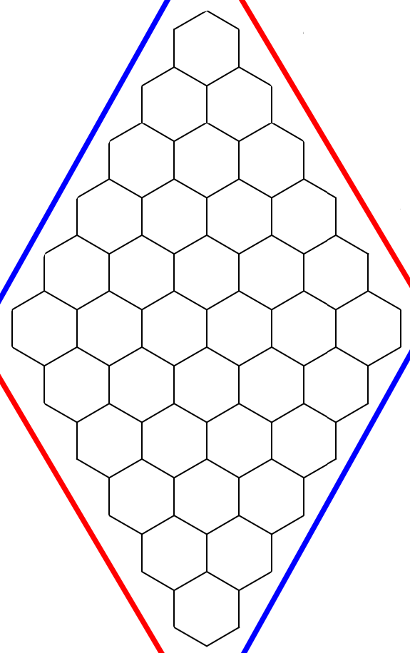
Hex is played on a rhomboidal board of hexagonal tiles by two players, Red and Blue, who alternate placing stones on the empty tiles of the board; to each player is assigned a pair of opposite board sides and the player who joins his assigned sides with a connected chain of stones of his respective colour is the winner.

2.1.1 Fundamental results
Remark 2.1.
Theorem 2.2 (Hex Theorem).
At a finite Hex position in which all the tiles are marked by either Red or Blue, at least one of the players has won.
The Hex Theorem is the result that carries the highest mathematical significance of finite Hex; [Gale, 1979] showed it to be equivalent to the Brouwer Fixed Point Theorem, which in turn was shown to be equivalent to the Jordan Curve Theorem by [Maehara, 1984] and [Adler et al., 2016].
In order to present the argument by [Gale, 1979], we need to mention the following simple graph-theoretic result.
Lemma 2.3.
A finite graph whose vertices have degree at most 2 is the union of disjoint subgraphs, each of which is either (i) an isolated vertex, (ii) a simple cycle, or (iii) a simple path.
Proof of Theorem 2.2.
Let be the graph induced by the edges on the Hex board with the addition of 4 edges ending in the vertices , as in figure 2.2(a).
Now, given a completely marked board, we present an algorithm to find a winning chain of stones.
Starting from , we construct a tour along following the rule of always proceeding along an edge which is the common boundary of a cell with a Red stone and a cell with a Blue stone; observe that the edge starting from does have this property, by considering the quadrants outside of the board as assigned to the players, see figure 2.2(b) for an application of this touring rule starting from all the vertices of .


Observe that this touring rule determines a unique path; suppose that the tour has proceeded along some edge and arrives at some vertex . Two of the three tiles incident to are those of which is the common boundary, hence one has a Red stone and the other a Blue stone; the third tile incident to may have a Red or a Blue stone, but in either case there is exactly one edge which satisfies the rule described.
As a consequence of starting from , we have that such a tour will never revisit any vertex of ; however, is finite and so the tour must terminate.
It is clear from the above that such a tour must describe a subgraph of whose vertices have degree at most 2; hence, by Lemma 2.3, the tour starting at can only be a simple path, thus ending at either or . Observe that each of these vertices is incident to either the NW Blue quadrant or the NE Red quadrant.
If, say, the terminal vertex of the described tour is incident to the NE quadrant, then Red has a winning chain which is incident to the edge tour starting in and joins the NE side with the SW side of the board; the other case for Blue is analogous. ∎
Remark 2.4.
Observe that this proof does not require any “right-left” orientation of the tour.
Moreover, we do not even require that the fully marked board is the ending position of some legal play.
Theorem 2.5.
There is no finite Hex position in which both players have won.
This Theorem is usually proved via an application of the Jordan Curve Theorem; we propose another visual proof by [Schachner, 2019].
Proof of Theorem 2.5.
Similarly to the previous proof, we add one distinguished vertex for each side of the board and an extra one.
Supposing for a contradiction that both Red and Blue win, we can use the two winning paths in the ending board position to construct the full graph with 5 vertices, as in figure 2.3.
However, such a graph cannot be planar; contradiction.

∎
Historical Remark 2.6.
According to [Hayward and Toft, 2019, pp. 7–8], Piet Hein was aware of this alternative proof; he realised that the (then unproved) Four Colour Theorem implied that there is no planar full graph with 5 vertices. He mentioned this as the foundation for his intuition behind the design of Hex.
Corollary 2.7 (No-tie property).
All plays of finite Hex end with exactly one winner.33 3 We can unambiguously say that plays end because they can last only for as many turns as there are tiles on the finite Hex board.
Proposition 2.8 (Strategy-stealing).
In finite Hex, the second player does not have a winning strategy.
Remark 2.9.
We observe the following basic properties of finite Hex.
- i.
It is never disadvantageous for any player to have an extra stone on the board,44 4 Note how in a dynamic game in which pieces can change position like Chess, for instance, having an extra piece that obstructs the escape of one’s king can facilitate a checkmate. Or observe that it is possible to construct dynamic game positions in which making more than one move in a turn can put a player at a disadvantage. as first observed by the discoverer in [Nash, 1952].
- ii.
There exists a rigid motion of the board into its opposite – that is, can be rotated, translated, and possibly reflected, into the board consisting of with each boundary segment assigned to the opposite player.
Proof of Proposition 2.8.
Suppose for a contradiction that Blue, the second player, has a winning strategy .
Let be the opposite strategy of , that is the corresponding strategy on the opposite board, in the sense of Remark 2.9.ii.
Now, let Red, the first player, place a stone on an arbitrary tile and then play according to ignoring the extra tile , so to pretend to play as second. If, at some turn, prescribes Red to play on , then Red can place a stone on another arbitrary tile and continue to play ignoring it.
Note that the strategy for Red is winning, exactly because is a second-player winning strategy and because ignoring his initial move can not obstruct his win, as observed in Remark 2.9.i.
But now both players can have a winning strategy; this is a contradiction by Corollary 2.7. ∎
Observe how the symmetry property of Remark 2.9.ii is crucial for the argument above; it would not be possible to let Red use Blue’s strategy otherwise, as the board, and so the relevant winning conditions, would have “looked different” to each of them.
A natural example of boards that satisfy condition 2.9.i. but fail to satisfy condition 2.9.ii. is that of asymmetric Hex boards.
Aiming to balance the game of Hex in favour of the otherwise losing second player, it seems reasonable to use asymmetric boards; however, it turns out that the player playing along the short edge of the board has such a strong advantage to be able to win even when playing second.
In fact, it is possible to pair the tiles of any Hex board so that the player joining the long edges wins by choosing, at each turn, the cell paired to the last cell taken by the opponent, as observed by [Gardner, 1988, §8]. When making the initial move, the player following this strategy can just make an arbitrary move as in the proof of Proposition 2.8.
This is clearer in the example of figure 2.4.

We will see in section 2.2.2 that a direct generalisation of this strategy will provide a drawing strategy for the second player in the game of Infinite Hex starting from an empty board.
2.2 Infinite Hex
It is immediate to generalise the board of Hex to the infinite plane; Infinite Hex is a class of games in which the two players, still Red and Blue, alternate placing their respective stones on the hexagons that tile the infinite plane.
Note that the hexagonal tiles of the Infinite Hex board are in bijection with , so that the players, at each turn, can choose to mark one of at most countably many tiles; hence, the game tree of any game of Infinite Hex can always be embedded in the full countable tree , as we need.
In other words, any position of Infinite Hex, including the positions with infinitely many stones already placed, is the initial position of a well-defined game of Infinite Hex.
We next discuss the definition of winning condition, which is less straightforward.
2.2.1 Winning condition
Since the Infinite Hex board has no edges to join, it is not immediately clear how to define a winning condition; we would like to “join the opposite infinite ends of the plane”, so we will now formalise this intuition.
Given a position , we aim to determine whether some given player has won. Moreover, we need to ensure that not both players win in a single play, so to comply with condition 1.2.v. in the definition of game.
We first need some definitions, which can be easily repeated for Blue; let be the Infinite Hex board and fix some position , that is an assignment of each cell of to either or no player, together with a turn indicator.
An infinite Red path, or Red -chain, is a function such that all the cells in the image of are marked by Red at and , are adjacent in for all .
We can now approach the condition to determine whether an infinite Red path is winning.55 5 We could require a winning path to be geodesic, so that the sub-path between any two tiles in is the shortest Red path between such tiles; however, it will be clear that if Red has a winning path, then Red also has a geodesic winning path.
Pick some cell and impose an orthogonal system of reference with origin in and axes directed from South to North and from West to East, as in figure 2.5(a).
Observe that, with some flexibility in the identification of the South-North columns, we can use these axes to obtain unique coordinates for each tile in ; this is best described by figure 2.5(b).


It can be useful to keep in mind the sketch of a general Red winning path in figure 2.6, while reading the following definitions.

Let be an infinite Red path.
Definition 2.10.
Given a system of reference centered at as above, we say that is winning with respect to if is eventually contained in the NE-quadrant and is eventually contained in the SW-quadrant of such reference system.
More precisely, we say that is winning with respect to if there is some such that if , then the coordinates of are both positive, while the coordinates of are both negative.
Definition 2.11.
We say that is a winning Red path if it is winning with respect to every choice of centre .
The winning condition for a Blue path is analogous, substituting NW for NE and SE for SW in Definition 2.10, as hinted by the key in figure 2.5.
Observe that the arbitrary choice of the origin for the reference system is necessary to avoid considering as wins paths which are bounded in one of the axes’ directions; otherwise we would not be able to assign consistently an outcome to the position in figure 2.7, in which the Red and Blue paths are unbounded towards North and South, but bounded in the WE-direction.
In fact, each path is winning for the relevant player with respect to several cells on the paths themselves, while neither path is winning with respect to the starred tile, for instance.

Remark 2.12.
By insisting in Definition 2.10 that the coordinates of have to be strictly positive, and of strictly negative, then we can define a path to be winning, equivalently to Definition 2.11, if it is winning with respect to each of its tiles; such a path cannot then be bounded in either of the axes’ directions.
We now show that the condition above is well-defined in the sense of defining disjoint winning conditions for the two players, as per Definition 1.2.v.
Proposition 2.13.
Not both players can win in a position of Infinite Hex.
Proof.
Suppose for a contradiction that is a position of Infinite Hex such that both Red and Blue have winning paths, respectively, and .
Pick some origin and let be the projections on the WE- and SN-axes centered at , so that the coordinates of a tile are .
Note that both paths and are winning, for the relevant players, with respect to ; hence there is some such that for we have that66 6 is the maximum of the two bounds given by Definition 2.11 for and .
Consider now the finite paths and ; we claim that they cannot be both connected.
Let be the smallest finite Hex board centered at and with the usual orientation, such that it contains both and .
Now, let be the maximally connected finite sub-paths of that extend, respectively, in ; we claim that they are both winning in , according to the usual finite Hex winning conditions, leading to a contradiction.
Observe that, by choice of , the ends of the path , i.e. and , are included in, respectively, the NE- and SW-quadrants of the reference system centered at .
As extends without getting out of the relevant quadrants, then is a Red winning path in the game of finite Hex played on .
An analogous argument can be made to show that is a Blue winning path in the game of finite Hex on , which leads to the contradiction needed, by Theorem 2.5. ∎
We conclude this section by presenting two “extreme” positions that motivated the choice of the definition of winning condition given and allowed to discard several other possible definitions. These positions are draws according to our definition, but can easily be considered wins by either or both players with weaker conditions.
In particular, observe how the Red path in figure 2.8 is unbounded in the NE-SW-direction, as desired, but also goes through the East-West pink band infinitely many times.

Moreover, the Red and Blue paths in figure 2.9 are unbounded in all directions; any coherent winning condition that identifies one of them as winning has to do the same with the other.

2.2.2 Normal Infinite Hex is a draw
In section 2.2.1 we provided a definition of winning positions, rather than plays; this is because the theory of transfinite game values developed in section 1.1 only applies to open games, and so we are mostly interested in applying such theory to the sub-class of games of Infinite Hex which are open for some designated player.
Nevertheless, we can consistently extend Definition 2.11 to all plays of Infinite Hex by dropping the finiteness condition; a player wins if he has a strategy with which he can eventually construct77 7 In at most countably many moves, as plays still have order type at most . an infinite path which is winning according to Definition 2.11, however his opponent plays.
Equipped with this new definition, we can ask the question: who wins from the initially empty position? We are particularly interested in clarifying whether the advantage of the first player in finite Hex carries on to Normal Infinite Hex, the game of Infinite Hex with the empty board as initial position.
We will show that this is not the case and that both players can force at least a draw from the empty board. However, we later conjecture in section 2.3.2 that the first player may still win if given some advantage, possibly of only one tile.
Let be a pairing of the tiles of the Infinite Hex board as depicted in figure 2.10; cells in the same pair have the same label. Note that pairs each cell with exactly one other cell.
Let be the second-player strategy, called mirroring strategy, induced by as follows; whenever Red, the first player, places a stone on a tile , then prescribes that Blue places a stone on the the tile paired with , according to .

Observe that is a well-defined strategy for Normal Infinite Hex. If Blue follows it since her first move, then Red will not be able to mark over the course of the play both tiles of any pair given by ; hence, at each turn, the tile indicated by to Blue will always be empty. Moreover, note that, following , Blue always places a stone in the opposite half-plane to where Red played immediately before, with respect to the East-West mirroring axis.
Remark 2.14.
Similarly to the Strategy-stealing argument of Proposition 2.8, we can adapt to be a first-player strategy.
Let be the pairing given by reflecting the pairing across some North-South axis.88 8 Observe that is essentially unique, given . Let be the strategy that prescribes Red to make an arbitrary initial move and then follow the (second-player) mirroring strategy induced by , possibly making arbitrary moves when the mirroring strategy prescribed to place a stone on a tile already marked by Red; this is because the mirroring strategy ignores the initial move and the subsequent arbitrary moves by Red.
Since the reflection of all possible winning paths for Red across a North-South axis gives exactly all possible winning paths for Blue, it is then clear that showing that is a drawing strategy for Blue implies that is a drawing strategy for Red.
Remark 2.15.
The pairing in figure 2.10 is called mirroring because it is not a symmetry and does not represent a rigid motion of the board. In particular, we obtain the Northern half-plane as the reflection across the mirroring axis of the Southern half-plane, followed by a translation by half a cell towards East; this translation is in effect “tearing” the plane.
Remark 2.16.
As already observed, when Blue plays according to , Red can mark at most one tile in each pair given by .
It follows that if Red constructs some winning path , then contains at most one tile in each pair given by , so that Blue can mark all the cells of , the mirroring of with respect to ; we call this the mirroring condition on .
Before proving the main result of this section, we make two observations.
Firstly, any Red path that crosses the mirroring axis of can only do so with two adjacent cells in the NW-SE-direction, that is the “wrong” direction for Red. This will be key for the argument, and is clear by inspection of figure 2.11.

Secondly, allows Blue to win, as long as Red plays appropriately bad. Observe that the position in figure 2.12 is winning for Blue and satisfies the mirroring condition of Remark 2.16 for the Red path.

Proposition 2.17.
In Normal Infinite Hex, is a drawing strategy for the second player.
Proof.
Suppose for a contradiction that Red has a winning strategy .
Letting Red play according to and Blue according to , Red will be able to construct a winning path99 9 Such path is only constructed after infinitely many turns, as described at the beginning of this section. which satisfies the mirroring condition of Remark 2.16, so that does not contain both tiles of any of the pairs of .
Now, we claim that cannot be a winning path. Observe that has to cross the East-West mirroring axis at least once. So, suppose that crosses the mirroring axis exactly once. We then expect a single Red intersection as in figure 2.11.
Since is winning for Red, then the semi-infinite sub-path of in the Northern half-plane will eventually go towards North-East; by definition of , Blue will correspondingly construct the mirrored sub-path in the Southern half-plane that eventually goes towards South-East, as in figure 2.13(a).
However, we also have that the sub-path of in the Southern half-plane must eventually go towards South-West, but if that is the case, then we can draw a finite Red path1010 10 This extra Red finite path is drawn directly on the board for the sake of the geometric argument; it is not part of the play. as in figure 2.13(b) so that we can identify a simple closed curve determined by adjacent Red stones, such curve is a Jordan curve which is intersected by a connected Blue path; this is a contradiction by the Jordan Curve Theorem.


Suppose now that crosses the mirroring axis more than once; cannot cross it exactly twice because it is a winning path, and in particular a connected path, thus assume that crosses the mirroring axis exactly thrice.
We expect to see three Red intersections of the mirroring axis as in figure 2.14(a); these were discussed before in figure 2.11.


Observe that the only way to construct such a path is to join with Red finite paths the ends labelled with , and with , and joining appropriate semi-infinite Red paths to the ends labelled and .
Such a construction is not possible due to the mirroring condition of Remark 2.16; observe in figure 2.14(b) how joining two ends in the same half-plane prevents one end in the opposite half-plane to be extended indefinitely.
These observations clearly hold by applying the Jordan Curve Theorem similarly to the above.
Observe that the argument for intersecting the mirroring axis three times can be easily adapted to any position in which intersects the mirroring axis a larger (odd) number of times.
Since can only intersect the mirroring axis finitely many times, as it is a winning path, we then conclude that cannot intersect the mirroring axis more than thrice, either. The proof is complete. ∎
Remark 2.18.
It is possible to prove Proposition 2.17 via a more involved argument by contradiction which reduces a Red winning path to a winning path for the disadvantaged player of a game of finite Hex on an asymmetric board.
In this sense, we can think of Infinite Hex as generalising the asymmetric variant of finite Hex, rather than the standard finite version.
2.3 Positional and stone-placing games
2.3.1 Positional games
Many popular board games belong to the class of positional games, which share the property of extra moves being always advantageous as in Hex,1111 11 See Remark 2.9.i. and whose simplest representative is the game of Tic-tac-toe.
Even though universally popular, we mention the rules of this game; in Tic-tac-toe two players, Naughts and Crosses, alternatively place their marks on a square board. The first player to mark three squares on a straight line wins, i.e. the first player to mark all 3 elements of any of 8 distinguished subsets of the board wins.
Note that the sets of board cells that allow the players to win are the same for both players.
We define such “Tic-tac-toe-like games” as in [Hefetz et al., 2014]; in order to additionally allow for infinite games, we define the following structure.
Definition 2.19.
A generalised hypergraph is a pair of sets , such that is the collection of vertices, and is the collection of hyperedges.
Note that from now on we will not distinguish between generalised hypergraphs and hypergraphs, which are usually defined stressing the finiteness of both the vertex and hyperedge sets.
Definition 2.20.
A positional game played on a hypergraph is a game such that the players alternatively mark previously unchosen elements of the vertex set , which represents the set of cells of the game board that are unmarked at the initial position.
The first player to mark all the vertices of some hyperedge in wins; here is called the collection of winning sets.
Recall from Remark 1.3 that a position in a positional game is an assignment of some of the board cells to the players, together with the history of moves and a turn indicator.
Remark 2.21.
Observe that, in Definition 2.20, specifying that only the first player to satisfy the winning condition is the winner ensures openness of the game for both players and is necessary to avoid ambiguity.
See for instance the Tic-tac-toe board position in figure 2.15; both players seem to be winning, but assuming that Crosses is the first player of the game, then we can say that, for any history of legal moves leading to that board position, the resulting position is a win for Crosses.

Remark 2.22 (Strategy-stealing).
Observe that Nash’s Strategy-stealing argument1212 12 See proof of Proposition 2.8. can be applied to show that any positional game played on is either a draw or a first-player win.
In fact, if the second player has a winning strategy, then the first player can use it after having made an arbitrary initial move, leading to a contradiction; this holds because both players have exactly the same winning conditions, which are represented by , and because in all positional games it is always advantageous to make an extra move, i.e. to choose one extra vertex.
Thus, the best outcome for the second player in a positional game is achieving a draw. For this reason, we do not lose generality when considering the class of games defined below.
Definition 2.23.
A Maker-Breaker game played on a hypergraph is a game in which Maker wins by choosing all the vertices of some winning set in , while Breaker wins by choosing at least one vertex of each winning set in .1313 13 A different definition could let Breaker win whenever Maker does not win; such a no-tie variant is not equivalent to our definition in the setting of infinite games. Not all vertices in may be marked over some plays and neither player may satisfy their original winning condition over such plays, so that we would consider such plays ties with our definition and wins for Breaker with the no-tie variant.
Remark 2.24.
Clearly, Breaker’s goal is precisely to prevent Maker from winning; it follows that a play of any Maker-Breaker game cannot allow both players to win.
Moreover, we can see that there is a duality between Maker and Breaker that preserves strategies, but not game openness.
Namely, take a Maker-Breaker game open for Maker and played on some hypergraph ; observe that such a game is equivalent1414 14 Equivalent from the point of view of the closed player. to the Maker-Breaker game not necessarily open for Breaker and played on the hypergraph , but with the players’ roles reversed, where
Observe that Breaker aims to mark at least one vertex in each of the winning sets in , so that does represent the correct winning condition in the game with the roles reversed.
Remark 2.25.
Recalling the no-tie property of finite Hex,1515 15 See Corollary 2.7. we observe that a finite Hex player who prevents the opponent from winning is equivalent to the player himself winning. In other words, the best offensive moves in finite Hex are exactly the best defensive moves, and vice versa.
Hence, we see that finite Hex is a Maker-Breaker game played on the hypergraph such that the vertex set is in bijection with the empty finite Hex board and is the collection of all the winning paths for Red, who corresponds to Maker.
What we mentioned in section 2.1.1 for asymmetric Hex boards is that no winning component for the player who is joining the short edges can avoid containing two cells paired with respect to the opponent’s strategy.
A weaker graph-theoretic property that follows from this pairing is that of proper 2-colourability of , where represents the relevant empty asymmetric board, and is the collection of winning paths for the disadvantaged player, who is losing; that is, can be coloured with two colours, say black and white, such that no collection of tiles that represents a winning path in is monochromatic.
Indeed, the cell pairing given by the mirroring strategy described in figure 2.4 is a particular case of such a proper 2-colouring, which is obtained by colouring with distinct colours the cells in each pair.
We prove the following result in appendix A.1.
Proposition 2.26.
Take some Maker-Breaker game played on a hypergraph such that is open for Breaker, and Maker is the first player to move. If Breaker has a winning strategy, so that he can play to take at least one vertex in each of Maker’s winning sets in , then is properly 2-colourable.
2.3.2 Biased Infinite Hex may not be a draw
Informally, our intuition of Infinite Hex is that, since the infinite board is ‘‘too large”, the advantage of placing the first stone is ‘‘too diluted”, and so an initial position with finitely many cells already marked by Red1616 16 Or even infinitely many, if placed “badly” enough. should not give a consistent advantage to Red, compared to the initially empty board, so that the game should result in a draw, as we saw in section 2.2.2.
However, adaptations of the mirroring strategy do not seem to be sufficient even in the case of just one extra stone for Red.1717 17 Of course, games of Infinite Hex biased in favour of the second player present essentially the same problem.
It seems reasonable to claim that no pairing strategy can be formulated. A possible proof could model Biased Infinite Hex as a Maker-Breaker game played on , where is the infinite board without the cells given to Red as advantage, and represents the winning condition for Red, the first player, and then assume for a contradiction that Blue has a drawing strategy, which would imply the proper 2-colourability of by Proposition 2.26; it is not clear how to get a contradiction from here.
The non-openness of the games of Biased Infinite Hex makes such problem less tractable.
We then formulate the following.
Conjecture 2.27.
A game of Infinite Hex with exactly one tile of the board assigned to Red at the initial position, and none to Blue, is a win for Red.
As an apparently easier problem, we also propose the following.
Conjecture 2.28.
A game of Infinite Hex with initial position as in figure 2.16 is a win for Red.

It is not difficult to see that from such a position Red can construct arbitrarily long, but finite, “prongs” that shoot out of the East-West infinite path; however, this is short of a definitive answer.
2.3.3 Stone-placing games
We will now prove that no infinite game values can be achieved in the following wider class of vertex-colouring games, that retain the property of extra moves being always advantageous for the player making them, which we first observed for finite Hex in Remark 2.9.i.
Definition 2.29.
A stone-placing game played on , where both and are hypergraphs, is a game in which the two players alternatively choose previously unchosen elements of the common vertex set ; at the initial position, all the vertices of the board are unmarked.
The hyperedge sets represent the winning conditions of, respectively, the first and the second player; that is, the winner is the player who chooses all the vertices of some winning set specified by his respective winning condition first.
Thus, we impose that both and are closed under taking supersets, without loss of generality.
Remark 2.30.
Note that Definition 2.29 does indeed generalise the other games defined previously in the current section 2.3.
Say that is a stone-placing game played on ; if , then is a positional game.1818 18 This clarifies why positional games are also known as Maker-Maker games.
We can see that if , where
then is a Maker-Breaker game in which Maker plays first; an analogous condition allows to be a Maker-Breaker game with Breaker playing first.
Remark 2.31.
If is a stone-placing game played on open for the first player, then every win by the first player is essentially finite, and so for any there is some finite such that . Thus, we can say that has a basis of finite sets; that is, there is such that is finite for each , which is not necessarily finite, and, for any , there is for some .
To express this more explicitly, say that a play is a win for the first player because he manages to mark all the vertices in some infinite winning set , then there is a finite , for some , which is completely marked by the first player over ; since each vertex is marked at some finite stage of the play,1919 19 This is a consequence of plays having order type at most . then the whole of is marked by the first player after finitely many turns and is an essentially finite play, as required by the openness of .
Hence, if is open for the first player, then we can regard the elements of the basis for as the “meaningful” winning sets, and we can thus assume that there are no “redundant” infinite elements in , without essentially changing . In particular, if all the elements of are finite, then is open for the first player.
If is open for the second player, then satisfies analogous conditions.
Analogously, we see that if a Maker-Breaker game played on is open for Maker, then has a basis of finite sets.
Dually, if is open for Breaker, then has a basis of finite sets, where is defined as above.2020 20 Recall the duality between Maker and Breaker discussed at page 2.24.
In particular, if both and its elements are finite, then is open for both players.
Remark 2.32.
We can generalise the mirroring strategy described in section 2.2.2 for Normal Infinite Hex, and at page 2.1.1 for finite asymmetric Hex boards, to give a condition that enables the second player2121 21 Note that an analogous result holds for the first player, who additionally makes an arbitrary initial move, as usual. We state the result for the second player because she is a priori at a disadvantage. to force a draw.
We propose another way to see that argument; the pairing for the the mirroring strategy determines an involution2222 22 Given a pairing of the tiles in the Infinite Hex board, we need the Axiom of Choice to define such an involution. of the infinite board ; note that has no fixed point, as each cell is paired with a different cell.
Take a winning path for Red and take its image under ; this will not necessarily be a winning path for Blue, exactly because the original tile pairing does not determine a rigid movement of the board; however, we have shown in section 2.2.2 that it will intersect Red’s path.
Observe that the intersection consists only of paired cells; hence, if the intersection is finite, then it has even size.
Proposition 2.33 (Mirroring).
Let be a stone-placing game played on . Suppose that there is a fixed-point free involution of the board, that is a bijective function such that and for all , and say that, for each , we have .
Then, the second player in can force a draw.
Proof.
Let the second player play as follows; at each turn, when the first player marks some vertex , then the second player chooses immediately after. Note that if was already chosen by the first player, then would have been previously taken by the second player, leading to a contradiction; thus, this strategy is well-defined.
Say that . Since , then ; moreover, since , then . Thus, and are distinct elements of ; we deduce that , if finite, has even size.
Following this strategy, the second player prevents the first player from choosing all the vertices in some hyperedge ; since , then the second player will always be able to counteract the moves of the first player, so that the first player will not be able to mark all the vertices in .
Therefore, the second player can force a draw. ∎
Remark 2.34.
Remark 2.35.
Note that the Strategy-Stealing argument2323 23 See Proposition 2.8. does not generally apply to this class of games, in fact, there is not always an automorphism of the vertices in such that each winning set in is sent to some winning set in .
2.3.4 Impossibility of infinite game values
Finite game values in Infinite Hex
Firstly, we show that all finite ordinals can be realised as the game values of some Infinite Hex positions through the use of virtual links.2424 24 These were first called angle-positions by [Hein, 1942], and then received this name by Claude Berge in 1977, according to [Björnsson et al., 2006, §7]; they are now part of the standard terminology used by Hex players [HexWiki, 2021].
The position in figure 2.17(a) is a bridge, as defined by [Browne, 2000, §12.3], which ensures that Red can join the two marked cells by choosing either of the two cells separating them. Blue can threaten this construction by occupying one of these two cells, and Red can simply respond by picking the remaining one, thus “realising” the virtual connection.


Joining two half-infinite lines by finitely many interlinked bridges allows to construct positions of any finite game value.
We present in figure 2.18 a position with value 5 for Red, two half-infinite linear components joined by 5 bridges, in which the virtual connections are highlighted.

Note that this position has infinitely many pieces already placed. More in general, since the winning player places only finitely many stones when starting from a position with defined game value, then it follows from the definition of winning condition that no position with defined game value can have only finitely many stones already placed.
Infinite game values
It can be reasonable to expect that some well-constructed open games of Infinite Hex can achieve an infinite game value; however, we will show that this is not possible by proving that Hex, as all stone-placing games, is an essentially local game.
Definition 2.36.
A dead region for some player in a stone-placing game, which is played on and has defined game value for the player’s opponent,2525 25 So that the game is clearly open for the player’s opponent. is some subset of the board such that, if all the vertices in are assigned to the (losing) player, then the game with the resulting initial position, which has the same turn indicator, still has value for the (winning) player’s opponent.2626 26 This definition is inspired by the concept of dead cells, which are usually defined in a more restrictive sense as cells that cannot influence the outcome of the game from a given position; see for instance [Björnsson et al., 2006, 3.1].
In other words, modifying the initial position of the game by assigning the cells of a dead region as advantage to the losing player does not substantially alter the game; even though the strategy of the winning player may change, the game value for such player does not vary.
Definition 2.37.
A stone-placing game, which has defined game value for some player, is essentially local for that player if there is a cofinite dead region of the board for that player’s opponent.
Remark 2.38.
An analogous definition can be made for essentially local positional games. Also, it is obvious that all finite games are essentially local.
For instance, see that all the empty tiles in figure 2.18, except for the 10 empty tiles which allow Red to realise the virtual links, belong to a dead region for Blue, hence that is the initial position of an essentially local game.
We aim to prove the following.
Theorem 2.39.
Any game of Infinite Hex with defined value for some player is essentially local for that player; thus, it has finite game value.
Observe that a game of Infinite Hex can be represented as a stone-placing game.
Suppose that Red is the first player to move in and say that and are hypergraphs in which the vertex set is in bijection with the board cells unchosen at the initial position of , and the hyperedges in represent all the possible winning paths for, respectively, Red and Blue. Note that the vertices of all hyperedges in and are unmarked at the initial position of .
We can see that can be interpreted as a stone-placing game played on , where the first player is Red and the second player is Blue.
It is now clear that Theorem 2.39 is a consequence of the following more general result.
Theorem 2.40.
Any stone-placing game with defined value for some player is essentially local for that player; thus, it has finite game value.
In order to highlight the symmetry between the first and second player, in the rest of this section stone-placing games will be played on by the players Open and Closed, who have winning conditions and , respectively.
Lemma 2.41.
Given any stone-placing game played on which has finite game value , we have that is essentially local for Open.
That is, there is a finite subset of the board such that Open has a strategy that allows him to win in at most turns by choosing vertices only in , and is a dead region for Closed.
Proof.
We prove this by induction on .
If , then there is nothing to prove, as Open has already won at the initial position and does not need to make any move. Trivially, .
Suppose that ; we consider this case for clarity of argument. Let be a winning strategy for Open realising this game value.
If Open is the next to move, then he can simply win by choosing a single vertex , as prescribed by ; in this case, is sufficient.
If instead Closed is the next to move, then suppose that he chooses some vertex , without winning. Then Open can again make a winning move by choosing some . If instead Closed decides to initially choose , then Open can still win by choosing the vertex prescribed by in that position. In either case, is as needed.
Suppose now that the Lemma is true for . Let have game value for Open, and let be a value-reducing strategy that realises this game value.
If Open is the next to move from the initial position, then, by definition of game value,2727 27 Definition 1.14. he can choose a vertex so to reach a position with game value . Then, by inductive hypothesis, there is a finite subset such that Open can win in at most moves by choosing vertices only from . In this case, is as needed.
If instead Closed is the next to move from the initial position, then suppose that he chooses some . Following , Open can mark some other to reach a position with game value at most ; by inductive hypothesis, there is a finite sub-board such that Open wins by choosing vertices only from it. Let .
Consider again the initial position of ; suppose that there are unchosen vertices2828 28 Note that both and are still unchosen at the initial position. in at the start, say . Now, take some and suppose that Closed decides to initially choose , to which Open replies by choosing some determined by , reaching a position of game value at most ; by inductive hypothesis, there is a finite sub-board such that Open wins by playing only on its vertices. Note that, in this case, the line of play of Open is only influenced by the moves made on the sub-board .
We claim that is a finite sub-board that satisfies the condition of the Lemma at the initial position of .
Suppose that Closed initially chooses an available vertex in , that is, he chooses for some . Open can reply by choosing the corresponding vertex , and subsequently win in at most more moves by playing on ; Open thus ends the game having chosen vertices only in , by construction.
Suppose now that Closed makes an initial move outside of , choosing some vertex (but possibly in ). Open can pretend to see as still unchosen and he can play as if Closed had made the phantom move of choosing . Hence Open can win by playing only on , as before. Observe that in this case the initial move by Closed does not obstruct Open’s play since Open wins by marking all the vertices of some such that , and that certainly does not depend on .
This concludes the proof of the Lemma. ∎
Lemma 2.42.
No stone-placing game open for some player has infinite game value for that player.
Proof.
Let be a stone-placing game played on , which is open for Open. Suppose for a contradiction that has infinite game value for Open; by Proposition 1.17, it is enough to assume that has game value for Open.
By definition of game value, Closed is the first to move in and can only reach positions with finite game value from the initial position.
So, suppose that Closed initially chooses some , reaching a position with finite value for Open. Now, by Lemma 2.41, there is a finite sub-board such that Open can win in at most turns by marking vertices only in . Let be a value-reducing strategy for Open that realises this in ; note that the moves prescribed by for Open only depend on the moves that take place on .
Suppose now that, from the initial position, Closed makes a different move .
Then, Open can ignore such move by Closed, and imagine instead that Closed had made the phantom move of choosing , and then play according to from such position imagined by Open.
Similarly to the situation in the proof of Lemma 2.41, Open can safely ignore Closed’s move in because allows him to win by playing only on , and so by marking all the vertices of some such that ; it is clear that Closed’s moves outside of cannot obstruct this goal.
It is important to note that, by playing outside of , Closed cannot aim to win, as he can only reach positions with defined game value for Open.
We have shown that, for an arbitrary initial move by Closed, Open can force a win in at most turns; thus, the position achieved by the initial move of Closed has game value bounded by . But the initial position had game value ; this is a contradiction. ∎
Proof of Theorem 2.40.
Remark 2.43.
Observe that the arguments above can be adapted to generalise the results to -player stone-placing games, once the definition of game value is extended to -player games.
By definition of omega one, we have the following immediate consequence of Theorem 2.40.
Theorem 2.44.
The omega one of any class of stone-placing games open for some player is at most .
We see that also Theorem 2.39 is now proved; following our previous discussion of Infinite Hex positions with finite game value, we can conclude by stating the result which answers the main question that motivated the present research.
Theorem 2.45.
The omega one of the class of open games of Infinite Hex is the smallest infinite ordinal, that is,
2.4 Other generalisations of Hex
It is not easy to intuitively capture the complexity of finite board games, so we now present explicitly some measurement of complexity for the finite games we mention in this work.
We mention the following estimates2929 29 From [van den Herik et al., 2002], and [Uiterwijk and Moesker, 2009] for TwixT. of the state-space and game-tree complexities of the different board games we are considering.
| Game | State-space complexity | Game-tree complexity |
|---|---|---|
| Checkers | ||
| Draughts | ||
| Chess | ||
| Hex | ||
| TwixT |
The Shannon game
The Shannon game is played on a graph with two distinguished vertices.
Rephrasing the definition of [Björnsson et al., 2006, §2], we can define this game as a Maker-Breaker game played on , such that is the set of non-distinguished vertices of and is the collection of paths that join the distinguished vertices of .
Usually, Maker is called Short, and Breaker is called Cut.
It should come as no surprise that Hex can be represented as a Shannon game.
TwixT
TwixT is a connection game played on a square lattice. The two players place stones on the vertices of such lattice and join two of their stones with an edge when they are opposite vertices of a rectangle.
The peculiarity of this game is that edges cannot intersect, so that the order in which moves are made have a great importance in determining the outcome of a game.
Moreover, even though TwixT looks rather different from Hex, it is actually a generalization of it. Thanks to the constructions provided by [Bonnet et al., 2016], we can simulate any Hex game on an appropriately filled TwixT board.
Observe that TwixT can be described as a particular edge-colouring game on the Knight’s graph, i.e. the graph obtained by joining the squares of a chessboard separated by a Chess knight’s move.
However, TwixT cannot be directly studied as a stone-placing game, and so we cannot apply our results to an infinite version of TwixT.
Chapter 3 Draughts
Also known as Checkers, Draughts is a board game that has a long tradition and many variants, all with the same core rules.
Some pieces, called pawns,11 1 Pawns are usually called pieces, which is a word that we will use to refer to both pawns and kings. are initially placed on the white squares22 2 We follow the common custom of displaying Draughts positions as played on the white squares of the board for clarity of presentation; we state the rules accordingly. of a chessboard, or draughtboard, usually of size , which we orient as usual. At the initial position, the pieces of Black are placed on the Southern side of the board and the pieces of White on the Northern side, as in figure 3.1.

At each turn, a player can move one of his pieces to one of the empty squares diagonally adjacent to it.
If a player’s piece is adjacent to an opponent’s piece, which in turn is adjacent to an empty square aligned with such two pieces, then the player can make a simple jump move letting his piece “jump” to the empty square, removing the “jumped” opponent’s piece from the board; see figure 3.2.


Moreover, if the player’s piece is, immediately after this jump, in a similar position, then the player can extend his move by making another jump; the resulting move is called an iterated jump. It is important to note that an iteration of jumps constitutes a single move, rather than multiple moves.
We refer to these two last types of move as jump moves.
In particular, Black pawns are only able to make such moves going strictly towards North; when a Black pawn reaches the Northernmost row of the chessboard, it is promoted to king, so that it can then make the moves described above in all directions. An analogous rule applies to White pieces.
The first player that is not able to make a move, either because he has no pieces left on the board or because he has no available legal moves, loses.
It is required in Draughts competitions that a player who can make a jump move at some turn must do so at that turn. Moreover, after a jump move, the piece just moved cannot be in a position from which another jump move could be possible.
In other words, if a player makes a piece jump, then he has to make it keep jumping, choosing which way to jump, until it reaches a position from which no more jumps are possible.
We can formalise this as follows.
Rule 3.1 (Forced Jump).
Each player must make jump moves, when they are legal.
Rule 3.2 (Forced Iteration).
No player can make a jump move which can be extended as an iterated jump move.
Observe that rule 3.2 allows players to make only maximal jump moves; in particular, it allows players to choose among distinct maximal jump moves. See for instance the position in figure 3.3, where Black can make a simple jump to the square labelled with a dagger, or make either of the iterated jumps to the starred squares; however, Black cannot make a simple jump to the square labelled with “” by rule 3.2.

Remark 3.3.
Rule 3.2 is justified by the fact that if a player makes one of his pieces jump without completing an available jump iteration, then that piece will be threatened, and likely captured at the next turn,33 3 Or certainly captured, in case that is the only jump move available to the opponent. by an opponent’s piece, as in the case of Black stopping on the square labelled “” in figure 3.3.44 4 Moreover, it is usually felt as an unfair advantage the possibility of a king to end a jump at the “back” of an opponent’s pawn, by which the king cannot be threatened.
3.1 Infinite Draughts
Analogously to Infinite Chess,55 5 See Example 1.12. Infinite Draughts is a game played on the infinite chessboard; in particular on its white squares, which are also in bijection with .
We can give a North-South orientation to the board so to maintain the difference between pawns and kings; however, all the pieces in the positions that follow are kings, unless otherwise specified.
Even though the rules of the game are simple and immediately generalise to the infinite case, we encounter a difficulty with the forced-iteration rule 3.2; observe the position in figure 3.4.

In fact, assuming only rule 3.1, if Black makes a jump move up the White infinite ladder in figure 3.4 and captures only finitely many White pieces, then White wins on the next move, as Black would stop his only piece in a square already threatened by White. Thus, if we applied strictly the forced-iteration rule 3.2, we would say that Black must make an infinitely iterated jump, capturing infinitely many White pieces in a single move.
Note that, on the next turn, White can move his only surviving piece at the bottom right, but, following that, Black has no pieces left on the board and thus loses; in fact, having made an infinitely iterated jump, the Black king is not on any of the squares of the infinite chessboard, thus it is not on the board anymore.66 6 In other words, the Black king effectively went to infinity.
It is clear that, for Black, making an infinitely iterated jump in the position of figure 3.4 is equivalent to admitting defeat; as we will consider positions in which Black also loses if he decides to make an infinitely iterated jump and we will want Black to delay his defeat as much as possible, we generalise the forced-iteration rule of Draughts as follows, in order to simplify the exposition in the next section 3.1.1.
Rule 3.4 (Finite Iteration).
If a player can make an iterated jump move, then he can only make a finite iteration of jumps.
Remark 3.5.
3.1.1 Embedding trees in the draughtboard
In this section, we will consider games of Infinite Draughts assuming rules 3.1 and 3.4, so that players must make jump moves when they can, and they can choose to iterate such jumps for at most finitely many times.
This will allow for simpler constructions in the rest of this section; we will consider different sets of rules in section 3.1.2.
Observe that, similarly to Infinite Hex, games of Infinite Draughts are not in general open, as it is possible to construct positions from which a player can win over an infinite play, but not at any finite stage of such play.
We therefore focus on the class of games of Infinite Draughts which are open for some designated player; we will prove the following.
Theorem 3.6.
Every countable ordinal arises as the value of an open game of Infinite Draughts. Hence,
We will prove this Theorem by constructing an argument closely related to the proof that the omega one of 3-dimensional Infinite Chess is , as shown by [Evans and Hamkins, 2014, §4].
We have already met a class of games with uncountable omega one; recall the class of climbing-through- games and Proposition 1.24.
We will now describe a way to construct, given any tree , a game of Infinite Draughts equivalent to the game of climbing-through-, so that a closed-player strategy for one game determines a closed-player strategy for the other game.
First, we ensure that the infinite draughtboard does provide enough space for our construction.
Keeping in mind the bijection between the white squares of the infinite chessboard and as specified by the system of reference presented in figure 3.5, we prove the following.

Proposition 3.7.
The full binary tree can be realised in .
Proof.
Recall that the full binary tree is the tree whose nodes all have exactly two children.
We now describe an algorithm to construct recursively the full binary tree.
For , we start the recursion with a single vertex.
For , we stack two copies of the same vertex, in red in figure 3.6, at a sufficient distance in order to join them to the original vertex.
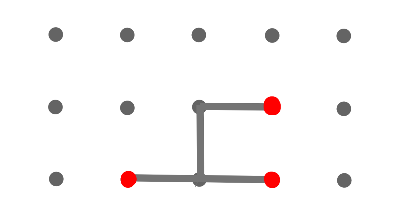
We then proceed similarly, given a subtree of , we construct by attaching a copy of to each of the leaves of the original we stack two copies of it to the right of the previous subtree at a sufficient distance from the original subtree and join each root of the new copies of to some leaf of the original ; this is always possible by stacking the new copies of far enough in the positive -direction; this is clear in the second recursive step pictured in figure 3.7.
We can see that the trees so constructed are binary and have leaves.
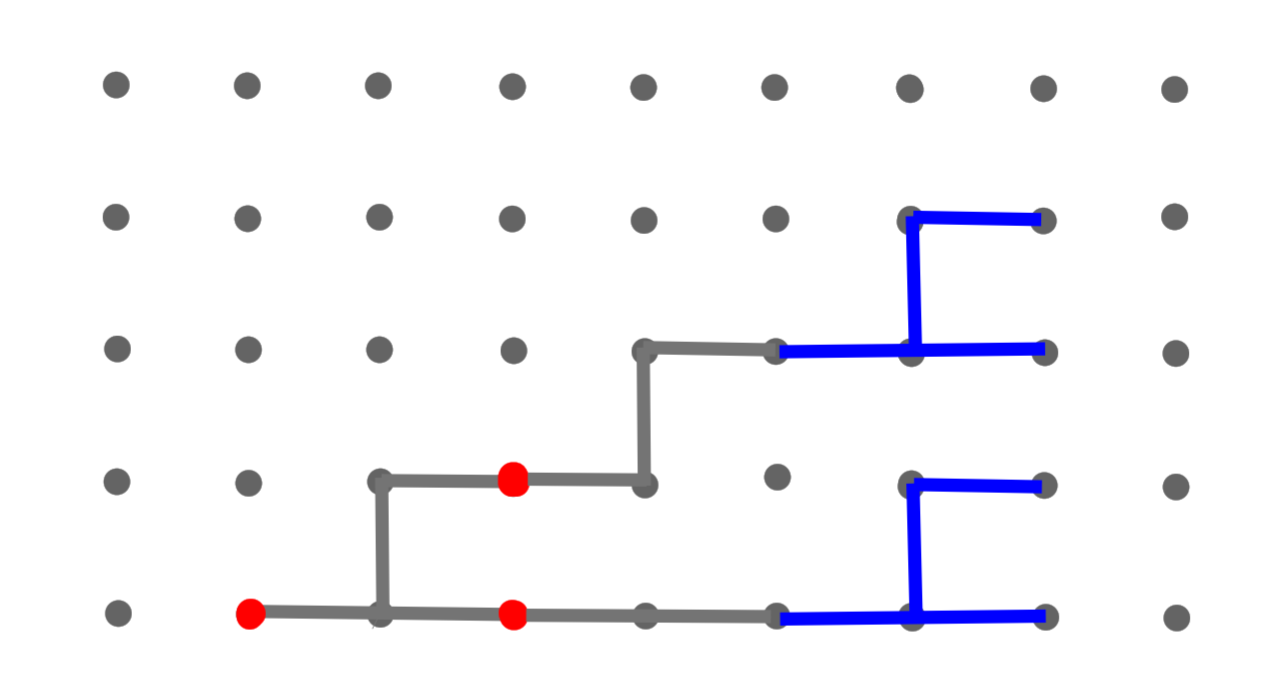
∎
Remark 3.8.
We have just shown that can be realised in a quadrant of the integer lattice ; however, at each step of the previous recursion, the new finite tree copies can be placed arbitrarily far in the positive direction of the -axis, so that the whole tree can be contained in a cone centered at the origin with an arbitrarily small non-zero angle at the centre.
We now define an arrangement of pieces on the draughtboard which will be key in the next argument.
Definition 3.9.
A White king tree is an arrangement of White kings on the infinite draughtboard, such that;
- i.
if a Black king is placed on a distinguished square, the root node of , diagonally adjacent to exactly one White king of the king tree, then each king of could be captured via a single jump move made by ; this ensures that the kings of are suitably alternated to empty squares and is connected;
- ii.
the nodes of are the empty squares of the board on which could end a, possibly not maximal, jump move; such jump move is unique for each node of ; this ensures that has no loops, and so really looks like a tree;
- iii.
there is no empty square of the board diagonally adjacent to 4 kings of ; so that the nodes of have degree at most 3, and so we can say that is a binary tree.
Following the usual graph-theoretic terminology, we say that a node of a White king tree is a leaf if it is the square reached by a Black king that makes a maximal jump move starting from the root of .
Theorem 3.10.
For any well-founded tree such that the game of climbing-through- has value for Observer, there is an open game of Infinite Draughts which has value for White; moreover, any strategy for Climber in the climbing-through- game determines a strategy for Black in , and vice versa.77 7 Such strategy correspondence could be made unique by imposing arbitrary conditions on them; it is not an issue in our discussion.
The initial position of comprises of a White king tree , a Black king on the root of , and White kings on all the leaves of ; the Black king is placed on the Southernmost non-empty square of the board and Black is the first to move.
Proof.
We will prove by transfinite induction on the rank of the tree that there exists a game of Infinite Draughts as described.
If , then White has already won and the empty board can be the trivial initial position of ; Black loses by being the first player.
If , then the children of the root node of are all leaves. If has only one child, then we can choose the position in figure 3.8 as the initial position of ; Black must make an initial jump move that ends on the square labelled with a dagger, and his only piece is then captured by White in the following turn.
Observe that figure 3.8 also shows what the leaves of the White king tree embedded in the draughtboard look like.

Similarly, if the root node of has any other finite number of children, we can iterate this construction; see figure 3.9 for the initial position of when has exactly 3 children.

Furthermore, if has (countably) infinitely many children, then we can let the initial position of be as in figure 3.10.

Observe that, in the last 3 figures presented, the Black king can only make legal maximal jump moves ending on the squares labelled with daggers.
In particular, in figure 3.10, Black must choose one of such squares; in fact, rule 3.4 prevents the Black king from making an infinitely iterated jump and thus remaining on the White ladder highlighted in green.
We can see that, given a strategy for Climber, that is a choice of a child node of , we can determine a strategy for Black in , that is a choice of jump move to the corresponding square labelled with a dagger.
Here, the fundamental observation is that we can see the initial position of , in which the Black king stands at the root node of the king tree, as corresponding to the initial position of the climbing-through- game, in which Climber stands on the root of ; moreover, we can see the Black king reaching a square labelled with a dagger as corresponding to the Climber moving up to the relevant node.
Hence, this construction allows us to determine the strategy correspondence of the Theorem.
Now, suppose that for all trees of rank there are games of Infinite Draughts with value as described.88 8 Recall that the rank of equals the game value of climbing-through- by Proposition 1.16.
First, suppose for simplicity that the root of has a single child ; if the maximal sub-tree of with root has rank ,99 9 is maximal in the sense that its vertex set is the same as the one of , except for . then has rank .
By induction, there exists some Infinite Draughts game of value as described by the Theorem; let be the arrangement of White kings at the initial position of , so that consists of a White king tree with White kings on the leaf nodes.
Let the initial position of be as in figure 3.11, in which we embed two copies of , so that each distinct copy of the king tree has one of the two starred squares as a root node.
Observe that this initial position of is constructible thanks to Proposition 3.7. The full binary tree can be embedded in a quadrant of the integer lattice and the king tree is binary, so the position of figure 3.11 can be constructed so that the Black king stands on the Southernmost non-empty square of the draughtboard. Observe that the embedded copies of may have more White kings than the original arrangement because Proposition 3.7 ensures constructibility, provided flexibility in the length of edges; this is not an issue because it is never advantageous for the Black king to end jump moves on nodes of the king tree which are not binary,1010 10 According to our definition of king tree, all the empty squares between white kings are nodes; however, the not properly branching nodes cannot be resting squares. such “stretched” copies of will be equivalent to the original with respect to the possible strategies available to Black.
In other words, Proposition 3.7 allows us to embed in the draughtboard king trees with the same graph-theoretic features of the original .

We can now describe the main line of play of Black, who is the first to move in .
The initial move by black is a jump move to the tile labelled with a dagger; we call it a resting square because the Black king can stop there without being captured by White at the next turn.1111 11 Observe that the Black king reaches the resting square by jumping over a White piece, hence it ends the move being adjacent to exactly 2 White pieces.
Then, we can see that the Black king is standing on the root of two White king trees, highlighted in orange, which each contain a copy of ; at the next turn, White can only move one piece from either of such king trees.1212 12 Or one of the kings on the leaves of such king trees.
At the next turn, Black can let his king make a jump move up the king tree whose pieces were not moved by White, and then play as in .
Since Black can then play in so to realise the game value , then the strategy just described realises the value . In fact, if the Black king does not stop on the described resting square, then it could stop on a non-resting square, leading to Black’s defeat on the next turn, or move past the first resting square and stop on some resting square higher up in one of the embedded copies of ; however, recalling the correspondence with the climbing-through- game, such a move would correspond to the Climber climbing up more than one edge per turn, causing a decrease in game value larger than necessary. Moreover, observe that White’s moves cannot really obstruct Black in the same way that the Observer does not obstruct the Climber by saying “OK”.
Hence, the main line of play for Black describes a well-defined strategy.
We have now all that we need to complete the proof; if the root of the tree has finitely many children, then we can iterate the previous construction so that, for each child of the root of , letting be the maximal sub-tree of rooted at , we can have, for each , a distinct resting square which is the root of two White king trees, both realising the White king tree of .
It should be clear that we can inductively construct the initial position of when the root of is infinitely branching, as in figure 3.12; a position for when the root of has finitely many children can be obtained by truncation of the green branch.

Observe that the discussion following figure 3.11 regarding the correspondence between the resting squares of the initial position of and the nodes of in climbing-through- easily extends to the finite and infinite branching positions of figures 3.11-3.12, with the only difference that White may respond to Black’s moves by moving pieces which Black does not intend to capture.1313 13 In other words, White could move pieces in irrelevant far branches of the king tree.
The proof is now complete. ∎
3.1.2 Further results
Computable positions
Note that we can define a position of Infinite Draughts to be a function that assigns to each white square of the chessboard a value to mark it as free or occupied by a piece, specifying if it is a pawn or a king and whether it is Black or White, in addition to specifying a turn indicator.
It is then immediate to consider computable positions as computable functions.
The following result is an adaptation of [Evans and Hamkins, 2014, Theorem 6] and is a consequence of Theorem 3.10.
Corollary 3.11.
There is a computable position of Infinite Draughts which is a win for a designated player if both players are constrained to play according to computable strategies, and is a draw otherwise.
We first recall a classic graph-theoretic result.
Lemma 3.12 (König’s Lemma).
Any infinite finitely-branching tree has an infinite branch.
Proof of Corollary 3.11.
Let be a computable infinite tree with no computable infinite branch; such trees exist by elementary results of computability theory.
Since is clearly finitely-branching, then is an infinite finitely-branching tree, and so has an infinite branch by König’s Lemma; such branch is not computable by definition of .
Even though is not well-founded, it still has branches of order type at most , so that we can apply the construction in the proof of Theorem 3.10 to construct a game of Infinite Draughts equivalent to the climbing-through- game.
It is clear that Climber has a winning strategy for the climbing-through- game, i.e. climbing up an infinite branch of ; however, has only non-computable infinite branches, so such strategy for Climber must be not computable.
By the strategic equivalence of climbing-through- with , we have that also Black has a non-computable drawing strategy in .
However, if Climber plays according to a computable strategy in climbing-through-, then he can only climb up a computable branch of , which must be finite by definition of . Correspondingly, if Black plays according to a computable strategy, then he will eventually reach in finitely many turns a leaf of the king tree in ; in such case, Black reaches an arrangement of White kings as in figure 3.8 and thus loses.
It is clear that any strategy is winning for White, as it is enough to require that White captures the Black king at the first mistake of Black, and make any other uninfluential move, otherwise; hence, we can say that White has a computable strategy which allows him to win in when Black plays according to any computable strategy.
This completes the proof. ∎
Tree nodes for different rules
We now focus on extending the previous results to games of Infinite Draughts that assume a less strict set of rules.
In particular, we will design nodes for the White king tree constructed in Theorem 3.10 with more structure than the one in figure 3.11.
All the positions in this chapter were kindly reviewed by Sergio Scarpetta, current World Champion of English Draughts (3-move variant), who confirmed the interpretations presented here, in particular the one regarding figure 3.15.
We observe that by allowing nodes to have fixed finite size in Proposition 3.7, we conclude that the full -ary tree can be embedded in the integer lattice .
Now that we have ensured to have enough space on the infinite draughtboard, we can present the node needed when dropping the forced jump rule 3.1, but maintaining the finite iteration 3.4.
Firstly, we need to ensure that the Black king actually starts jumping on the White king tree, so that the root of the king tree needs two extra guardian White kings, as in figure 3.13, where Black immediately loses by making an initial non-jump move; this was not needed in the previous root configuration.

Even though the Black king will still find it disadvantageous to stop on non-resting squares, we still need to ensure that the Black king does not get off-track, that is out of the king tree, when making a move from a resting square; that is exactly why we add two guardian White kings to the king tree branching node, which are highlighted in yellow in figure 3.14.

Remark 3.13.
Observe that when the Black king is on some resting square, White could move one of the guardian kings to a square adjacent to the Black king, offering it the possibility to go off-track.
The interesting thing to note is that White would make such a move only when, following the Black king going off-track, White could reach a position of value lower than the ones reachable by allowing Black to play as usual; such a situation means exactly that it is not advantageous for Black to go off-track.
This is enough to say that, with optimal play, Black will not capture a guardian king moved by White. In other words, White moves guardian kings only when that is uninfluential, exactly as the Observer says “OK” in the climbing-through- game.
Recalling that we stated rule 3.4 in order to avoid discussing infinitely iterated jumps, we are now ready to drop it and only assume the forced iteration rule 3.2 with its strict interpretation in Infinite Draughts.
In other words, we now assume that players are not obliged to make jump moves, but, if they do make a jump move, then they can only make maximal jumps, which include infinitely iterated jumps.
This complicates the structure of the nodes of, what we should now call, extended king tree constructed as in the proof of Theorem 3.10; in fact, we will require the Black king to reach a resting square and possibly make a non-jump move, before continuing to climb the extended king tree.
Observe in figure 3.15 the first node that the Black king can decide to pick; it is a 7-branching node, so that each branch leads to an equivalent extended tree, as for the binary case in the original argument.

Remark 3.14.
It may be possible to further simplify the node in figure 3.15; however, the one presented is likely to be the minimal node when reintroducing the forced jump rule.
Observe that the branches are coloured red or orange depending on their row parity.
Suppose that the Black king decides to pick that first node, rather than continuing on the green ladder, and so ends the initial jump move on the resting square labelled with a dagger.
The main line of play for Black is as follows. After White’s non-jump move, move the Black king to the starred square adjacent to an external triplet of branches which was not modified by White; White can then move a piece from only one of the red branches next to the Black king, which can then make a jump move to climb up the other, going to another node.
There are several ways in which White could interfere with this strategy, and we will see that they are uninfluential in terms of reducing the game value.
Even though players are not forced to make jumps when legal, White might offer the possibility of a jump move to Black.
Recalling that jumps must be maximal, we have that, if White moves a king so that Black can make a jump towards North-West, then Black can decide to deviate from the main line of play to go up the orange branch, in which case Black leaves the node reducing the value by 1 rather than 2, which is still a positive outcome for Black.
White could also offer possible jump moves towards NE or SW by moving a White king to a starred tile; if Black takes up the offer, then he simply jumps up the relevant external orange branch.
Moreover, if White moves a king to the South-East of the Black king, then it is likely to be advantageous for Black to make such a jump move and go to choose another node up the green branch; this would correspond to the Observer allowing the Climber to go back down to the tree root and make a different choice.
Following White’s response to Black’s initial move, Black may decide to move his king to a non-starred square.
If the Black king is moved to the North-West of the resting square, then it would be captured by White on the next move.
If instead the Black king is moved towards South-East, that is “backwards”, then White can place a king to the North-West of the (original) resting square, and then we can see that the Black king is trapped, also thanks to the guardian kings highlighted in yellow.
Finally, the only other option available to White when Black is standing on a starred square is moving the piece at the bottom of the external orange branch next to the Black king; by an analogous argument to Remark 3.13, we have that White would make that move only if that does not affect Black’s play.
With this, we conclude our discussion of Infinite Draughts.
Appendix A Appendix
A.1 2-colourability in Maker-Breaker games
We prove the following result, which is adapted for any generalised hypergraph from [Hefetz et al., 2014, Proposition 2.3.1].
Proposition A.1.
Take some Maker-Breaker game played on a hypergraph such that is open for Breaker, and Maker is the first player to move.11 1 Note that this argument relies on the fact that Breaker’s winning strategy is a second-player strategy. If Breaker has a winning strategy, so that he can play to take at least one vertex in each of Maker’s winning subsets in , then is properly 2-colourable.
Proof.
Suppose that is a winning strategy for Breaker, and let Breaker play according to it, so that at least one vertex in each hyperedge in is chosen by Breaker, who does that after finitely many turns.
Moreover, let Maker make an arbitrary initial move, which cannot be disadvantageous, and then play according to , as if the arbitrary move was not placed on the board. Whenever prescribes to choose a vertex already marked by Maker himself, then he can analogously make another arbitrary move. Note that Maker’s extra move is the only one that the strategy does not consider, thus will never prescribe Maker to choose a vertex already marked by Breaker.
Then, Maker will satisfy Breaker’s winning condition; that is, given any hyperedge in , Maker will choose one vertex from it, and will do that after finitely many turns.
Note that if is infinite, then not all vertices will necessarily be chosen by either player at any finite stage; if a vertex does not belong to any hyperedge, then it will never be chosen.
Moreover, if is uncountable, then at most countably many vertices will be marked by either player, as all plays are countable sequences of moves, by Definition 1.2.iv.
However, by the definition of , all hyperedges comprise one vertex marked by Maker and one by Breaker, both chosen at some finite stages of the game.
Assign the colour white to all the vertices marked by Maker, and the colour black to all the vertices marked by Breaker or left unchosen.22 2 So that we do not need the Axiom of Choice here.
This assignment is a proper 2-colouring of , as needed. ∎
A.2 Strategy-stealing in stone-placing games
We generalise the symmetry condition of the finite Hex board highlighted in Remark 2.9.ii to construct the Strategy-stealing argument for stone-placing games.
Definition A.2.
A game is strictly not open for one player if that player can only win by playing for infinitely many turns; that is, if the winning condition of that player has empty interior, and so does not contain any basic open set, within the space of plays.
Proposition A.3 (Strategy-stealing).
Let be a stone-placing game played on , strictly not open for both players. Say that there is a fixed-point free involution of the board . Suppose that is such that for each there is some for which .
Then, the second player in does not have a winning strategy.
Hence, we can informally interpret the involution as a symmetry (or better, a reassemblage) of the board that allows the first player to act as the second player on the new board.
Proof of Proposition A.3.
Let the first player make an arbitrary initial move, which is advantageous, and then play in the following way; when the second player chooses a vertex , then the first player, in the next turn, marks .
Note that is infinite by strict non-openness of , and that the second player will mark all the vertices of , each after finitely many turns. Thus, the first player will eventually mark all the vertices of .
Therefore, the first player will also win by marking all the vertices of some such that , which is a contradiction. ∎
Remark A.4.
Observe that we cannot relax the assumption of strict non-openness in Proposition A.3.
Otherwise, the second player could pick a finite , which preferably does not contain the initial move of the first player, and then could proceed to mark all the vertices in , so that the first player would be able to fully satisfy his winning condition only with his move that follows the last move of the second player; that is a move too late, so that the second player actually wins.
Note that strengthening the condition by imposing that the involution is such that for each there is some for which is still not enough; there could be an appropriate order in which the second player could mark the vertices of a finite that defeats the opponent.
References
- [Adler et al., 2016] Adler, A., Daskalakis, K., and Demaine, E. (2016). The complexity of hex and the jordan curve theorem. In Chatzigiannakis, I., Mitzenmacher, M., Rabani, Y., and Sangiorgi, D., editors, 43rd International Colloquium on Automata, Languages, and Programming (ICALP 2016), number XXX in Leibniz International Proceedings in Informatics. Dagstuhl Publishing.
- [Björnsson et al., 2006] Björnsson, Y., Hayward, R., Johanson, M., and van Rijswijck, J. (2006). Dead cell analysis in hex and the shannon game. In Bondy, A., Fonlupt, J., Fouquet, J., Fournier, J., and Ramírez Alfonsín, J., editors, Graph Theory in Paris, Trends in Mathematics, pages 45–59. Birkhäuser Basel.
- [Bonnet et al., 2016] Bonnet, É., Jamain, F., and Saffidine, A. (2016). On the complexity of connection games. Theoretical computer science, 644(C):2–28.
- [Browne, 2000] Browne, C. (2000). Hex strategy: making the right connections. CRC Press.
- [Conway, 1996] Conway, J. H. (1996). The angel problem. In Nowakowski, R. J., editor, Games of No Chance, volume 29 of Proceedings of the MSRI Workshop on Combinatorial Games, pages 3–12. Cambridge University Press.
- [Evans and Hamkins, 2014] Evans, C. D. A. and Hamkins, J. D. (2014). Transfinite game values in infinite chess. Integers, 14:Paper No. G2, 36.
- [Evans et al., 2017] Evans, C. D. A., Hamkins, J. D., and Perlmutter, N. L. (2017). A position in infinite chess with game value . Integers, 17:Paper No. G4, 22.
- [Gale, 1979] Gale, D. (1979). The game of hex and the brouwer fixed-point theorem. The American Mathematical Monthly, 86(10):818–827.
- [Gale and Stewart, 1953] Gale, D. and Stewart, F. M. (1953). Infinite games with perfect information. In Kuhn, H. W. and Tucker, A. W., editors, Contributions to the Theory of Games, volume II, pages 245–266. Princeton University Press.
- [Gardner, 1988] Gardner, M. (1988). Hexaflexagons and other mathematical diversions – The First Scientific American Book of Puzzles and Games. University of Chicago Press.
- [Hayward and Toft, 2019] Hayward, R. B. and Toft, B. (2019). Hex, Inside and Out: The Full Story. CRC Press.
- [Hefetz et al., 2014] Hefetz, D., Krivelevich, M., Stojaković, M., and Szabó, T. (2014). Positional Games. Oberwolfach Seminars. Springer Basel.
- [Hein, 1942] Hein, P. (1942). Vil de laere polygon? Politiken, Copenhagen, Dec. 26. Translated into English by [Hayward and Toft, 2019, §3.1].
- [HexWiki, 2021] HexWiki (2021). Strong connection. https://www.hexwiki.net/index.php/Strong_connection (accessed 1st July 2021).
- [Kunen, 2013] Kunen, K. (2013). Set theory, volume 34 of Studies in Logic. College Publications, London, revised edition.
- [Maehara, 1984] Maehara, R. (1984). The jordan curve theorem via the brouwer fixed point theorem. The American mathematical monthly, 91(10):641–643.
- [Máthé, 2007] Máthé, A. (2007). The angel of power 2 wins. Combinatorics, Probability and Computing, 16(3):363–374.
- [Nash, 1952] Nash, J. (1952). Some games and machines for playing them. Technical Report D-1164. Rand Corporation. https://www.rand.org/content/dam/rand/pubs/documents/2015/D1164.pdf.
- [Schachner, 2019] Schachner, M. (2019). The game of hex: a study in graph theory and algebraic topology. Mathematics REU 2019. University of Chicago. http://math.uchicago.edu/~may/REU2019/REUPapers/Schachner.pdf.
- [Uiterwijk and Moesker, 2009] Uiterwijk, J. and Moesker, K. (2009). Mathematical modelling in twixt. In Löwe, B., editor, Proceedings Logic and the Simulation of Interaction and Reasoning 2 Workshop (LSIR2), pages 29–35. Pasadena: IJCAI.
- [van den Herik et al., 2002] van den Herik, H., Uiterwijk, J. W., and van Rijswijck, J. (2002). Games solved: Now and in the future. Artificial Intelligence, 134(1):277–311.