Strategyproof and Proportionally Fair
Facility Location

Haris Aziz Alexander Lam Barton E. Lee Toby Walsh Thanks: UNSW Sydney, Australia. Email: haris.aziz@unsw.edu.au Thanks: City University of Hong Kong, Hong Kong. Email: alexlam@cityu.edu.hk Thanks: ETH Zürich, Switzerland. Email: barton.e.lee@gmail.com Thanks: UNSW Sydney and Data61 CSIRO, Australia. Email: t.walsh@unsw.edu.au Affiliation: Affiliation: Latest version here Affiliation: First posted: 22nd October 2021.

Abstract

We focus on a simple, one-dimensional collective decision problem (often referred to as the facility location problem) and explore issues of strategyproofness and proportionality-based fairness. We introduce and analyze a hierarchy of proportionality-based fairness axioms of varying strength: Individual Fair Share (IFS), Unanimous Fair Share (UFS), Proportionality (Freeman et al. 2021, as in), and Proportional Fairness (PF). For each axiom, we characterize the family of mechanisms that satisfy the axiom and strategyproofness. We show that imposing strategyproofness renders many of the axioms to be equivalent: the family of mechanisms that satisfy proportionality, unanimity, and strategyproofness is equivalent to the family of mechanisms that satisfy UFS and strategyproofness, which, in turn, is equivalent to the family of mechanisms that satisfy PF and strategyproofness. Furthermore, there is a unique such mechanism: the Uniform Phantom mechanism, which is studied in Freeman et al. 2021. We also characterize the outcomes of the Uniform Phantom mechanism as the unique (pure) equilibrium outcome for any mechanism that satisfies continuity, strict monotonicity, and UFS. Finally, we analyze the approximation guarantees, in terms of optimal social welfare and minimum total cost, obtained by mechanisms that are strategyproof and satisfy each proportionality-based fairness axiom. We show that the Uniform Phantom mechanism provides the best approximation of the optimal social welfare (and also minimum total cost) among all mechanisms that satisfy UFS.

1 Introduction.

Facility location problems are ubiquitous in society and capture various collective scenarios. Examples include electing political representatives (Border and Jordan 1983; Feldman et al. 2016; Moulin 1980), selecting policies (Barberà and Nicolò 2021; Dragu and Laver 2019; Kurz et al. 2017), deciding how to allocate a public budget (Freeman et al. 2021), and deciding the location or services provided by public facilities (Schummer and Vohra 2002). Two key concerns in such problems are that the selection process may be vulnerable to strategic manipulations and/or fail to guarantee “fair” outcomes. In this paper, we simultaneously examine the issues of strategyproofness and fairness for the facility location problem.

In the facility location problem, each agent is viewed as a point on an interval. Depending on the motivating setting, the point could reflect the agent’s physical location, political position, or social preference. Each agent has symmetrically single-peaked preferences and prefers the collective outcome to be near their own position. The goal of the collective decision problem is to take agents’ preferences (positions) into account to find a reasonable collective outcome (the location of the facility).

The facility location problem (or the one-dimensional collective decision problem) is one of the most fundamental problems in economics, computer science, and operations research. It takes a central place in social choice theory as single-peaked preferences are one of the key preference restrictions that circumvent the infamous Gibbard-Satterthwaite theorem (Gibbard 1973; Satterthwaite 1975), which says that in general social choice, no unanimous and non-dictatorial voting mechanism is strategyproof. Furthermore, despite the unidimensional setting appearing restrictive, it is well suited to many real-world problems—most prominently, deciding the level of provision of a public good (Barberà and Jackson 1994; Cantala 2004, see, e.g.,). When agents have single-peaked preferences, the mechanism that returns the median voter’s position is unanimous, non-dictatorial, and strategyproof (Moulin 1980, see,). This seminal result has been discussed in hundreds of papers. Despite the importance of the median mechanism for the facility location problem, it does not satisfy several fairness concepts that are inspired from the theory of fair division and proportional representation. We focus on the following research questions.

For the facility location problem, what are natural fairness concepts? How well can these fairness concepts be achieved by strategyproof mechanisms? For strategyproof mechanisms that satisfy one of these fairness concepts, which mechanism performs optimally in terms of maximizing social welfare or minimizing total cost? Which mechanisms achieve fairness in equilibrium?

Our contributions are four-fold. First, we consolidate a number of fairness axioms from the literature, explicitly describe their relations and establish the compatibility—and, in some cases, incompatibility—of strategyproofness with these fairness concepts. We propose a new concept called proportional fairness (PF) that is based on the idea that the distance of a facility from a group of agents should depend both on the size of the group as well as how closely the agents are clustered. We also analyze existing axioms from the literature on fair division, participatory budgeting, and proportional representation such as proportionality, unanimous fair share (UFS), individual fair share (IFS), and unanimity. Our PF axiom is the strongest of these; Figure 1 describes the relationship between all the fairness axioms that we study.

Refer to caption — Figure 1: Relations between axioms. An arrow from (A) to (B) denotes that (A) implies (B). All relations are strict.

Second, we present two characterization results. We characterize the family of strategyproof mechanisms that satisfy unanimity, anonymity, and IFS. We then identify a specific mechanism, called the Uniform Phantom mechanism, that uniquely satisfies strategyproofness, unanimity, and proportionality. We also prove that the Uniform Phantom mechanism uniquely satisfies strategyproofness and UFS. Since we show that the Uniform Phantom mechanism also satisfies PF (and because PF implies UFS), we obtain as a corollary that the Uniform Phantom mechanism is the only strategyproof mechanism satisfying PF. Therefore, within the class of strategyproof mechanisms, PF and UFS collapse to the same property—in contrast, IFS is markedly weaker, even within the class of strategyproof mechanisms.

Third, we consider the fairness of outcomes under strategic behavior when a mechanism is not strategyproof. We prove that if a mechanism satisfies continuity, strict monotonicity, and UFS, then a pure Nash equilibrium exists, and every (pure) equilibrium under the mechanism satisfies UFS with respect to agents’ true locations. One mechanism in this class is the Average mechanism, which locates the facility at the average of all agents’ reported locations. Furthermore, for mechanisms satisfying continuity, strict monotonicity, and UFS, the equilibrium outcome leads to a facility location that equals the facility location of the Uniform Phantom mechanism when agents report their true location. Thus, our equilibrium analysis of continuous, strictly monotonic, and UFS mechanisms provides an alternative characterization of the Uniform Phantom mechanism.

Lastly, we take an approximate mechanism design perspective (Nisan and Ronen 2001; Procaccia and Tennenholtz 2013). We explore how well the maximum social welfare and minimum total cost can be approximated when fairness axioms and strategyproofness are imposed. Our goal is to identify mechanisms that deliver the best approximation guarantees while also satisfying strategyproofness and the corresponding fairness axioms (such as IFS and UFS). We first establish a stark negative result for the total cost approximation. Any strategyproof, anonymous, and unanimous mechanism that satisfies IFS has approximation ratio of $n-1$ , which is unbounded as $n$ grows. Because IFS is our weakest fairness axiom when strategyproofness is imposed, the total cost approximation analysis fails to distinguish any difference between the mechanisms that we focus on. We then turn to social welfare approximation where we establish more positive and nuanced results. Intuitively, imposing UFS leads to a strictly worse approximation ratio than if only IFS is imposed and, in either case, the best approximation guarantee is bounded. We identify strategyproof mechanisms that provide the best approximation of the maximum social welfare among all (not necessarily strategyproof) mechanisms that satisfy either IFS or UFS. In the latter case of satisfying UFS, the Uniform Phantom mechanism achieves this best approximation. In this sense, the fairness axioms impose a greater cost on the social welfare approximation guarantees than the strategyproofness requirement.

1.1 Related literature.

Facility location problems.

The facility location problem has been studied extensively in operations research, economics, and computer science. As is common in the economics literature, our paper takes a mechanism design approach. We assume an incomplete information setting, where agents have privately-known utility functions (and, hence, peak locations) and can strategically (mis)report their peak location. The problem is to design a mechanism that is strategyproof and achieves a “desirable” facility location with respect to the agents’ true locations. Moulin 1980’s (Moulin 1980) seminal work characterizes the family of strategyproof and Pareto efficient mechanisms when agents have single-peaked preferences. In our paper, agents have single-peaked preferences that are also symmetric, i.e., agents prefer the facility to be located closer to their location regardless of whether it is to left or right of their location; therefore, our setting is closer to Border and Jordan 1983. Border and Jordan 1983 characterize a strict subfamily of strategyproof mechanisms, which includes the family of strategyproof and unanimous mechanisms (Border and Jordan 1983 also extend their results to higher dimensions). Massó and Moreno De Barreda 2011 formalize the connection between the mechanism design problem in settings where agents have single-peaked preferences and settings where agents have symmetrically single-peaked preferences.

Since Moulin 1980 and Border and Jordan 1983, numerous scholars have explored open-questions related to these characterizations (Barberà and Jackson 1994; Barberà et al. 1998; Ching 1997; Jennings et al. 2021; Massó and Moreno De Barreda 2011; Peremans et al. 1997; Weymark 2011, see, e.g.,). Others have explored extensions and variations of the facility location problem. For example, Nehring and Puppe 2006; Nehring and Puppe 2007 relax the assumption that agents have single-peaked preferences; Miyagawa 1998; Miyagawa 2001 and Ehlers 2002; Ehlers 2003 extend the facility location problem to consider locating multiple facilities; Aziz et al. 2020b; Aziz et al. 2020a introduce capacity constraints into the problem; Jackson and Nicolò 2004 introduce interdependent utilities; Cantala 2004 introduces an outside option; and Schummer and Vohra 2002 extend the facility location problem to a network setting. For a recent survey of the computational social choice literature on facility location problems, see Chan et al. 2021. Our paper contributes to this literature by formalizing a hierarchy of “proportionality-based fairness” axioms for the facility location problem and characterizing families of strategyproof and fair mechanisms within each layer of the heirarchy. Additionally, in Section 5, we explore the equilibrium properties of non-strategyproof mechanisms. We obtain results that complement those of Renault and Trannoy 2005; Renault and Trannoy 2011 and Yamamura and Kawasaki 2013 (further details provided in Section 5).

There is also an extensive literature in operations research and computer science that studies the facility location problem within a complete information setting. These literatures largely focus on issues of computational complexity and approximation and, therefore, are not directly relevant to the present paper (Brandeau and Chiu 1989; Zanjirani Farahani and Hekmatfar 2009, for an overview, see).

Fairness in collective decision problems.

Issues of fairness in collective decision problems have been studied in a variety of contexts (Dummett 1997; Mill 1861; Nash 1950; Nash 1953; Rawls 1971; Sen 1980; Shapley 1953; Yaari 1981, see, e.g.,). Most closely related to the present paper are the social choice and computational social choice literatures (Arrow et al. 2010; Aziz et al. 2019b; Endriss 2017; Faliszewski et al. 2017; Klamler 2010; Laslier and Sanver 2010, for an overview, see). We formalize a hierarchy of fairness axioms for the facility location problem that are conceptually related to proportional representation. As will be discussed in Section 3.1, our axioms can also be motivated by—and connect with—notions of stability in cooperative game theory, such as the “core” (Scarf 1967, see, e.g., ). Two of our fairness axioms (IFS and UFS) are translations of the “individual fair share” and “unanimous fair share” axioms, which appear in fair division and participatory budgeting problems (Aziz et al. 2019a; Moulin 2003), into the facility location problem. In addition, we utilize a natural axiom of proportional representation, called “proportionality”, which is explored in the context of participatory budgeting by Freeman et al. 2021. Beyond translating existing notions of fairness into the facility location problem, we also introduce the new axiom of “Proportional Fairness” that is stronger than all of the aforementioned axioms.

Our approach contrasts with a number of facility location papers that attempt to obtain outcomes that achieve (or approximate) the egalitarian outcome, i.e., maximizing the utility of the worst off agent (Procaccia and Tennenholtz 2013, see, e.g.,). Mulligan 1991 notes that the egalitarian objective is sensitive to extreme locations and recommends distributional equality as an underlying principle for considering equality measures. When placing multiple facilities, several new concepts have been proposed for capturing proportionality-based fairness concerns (Bigman and Fofack 2000; Jung et al. 2020, see, e.g.,). However, these concepts are equivalent to weak Pareto optimality or unanimity when there is only one facility. For the single-facility problem, Zhou et al. 2022 recently examined the issue of welfare guarantees for groups of agents. Our approach and results differ in that we consider the classic facility location problem whereas Zhou et al. 2022 overlay it with additional information that places agents in predetermined groups.

In the context of the facility location problem, our paper characterizes strategyproof and “fair” mechanisms. Some of our results directly relate to those of Freeman et al. 2021. In the context of participatory budgeting, Freeman et al. 2021 explore the problem of designing strategyproof mechanisms that satisfy proportionality. One of their key results (Proposition 1) applies to the facility location problem and shows that there is a unique anonymous, continuous, strategyproof and proportional mechanism, which is called the Uniform Phantom mechanism. Like our paper, Freeman et al. 2021’s (Freeman et al. 2021) setting assumes that agents have single-peaked and symmetric preference. Jennings et al. 2021 provide a similar characterization of the Uniform Phantom mechanism in the setting where agents have single-peaked (and possibly asymmetric) preferences. Our paper differs in focus and provides a broader treatment of issues of fairness and strategyproofness in facility location problems; for example, we characterize a larger family of strategyproof mechanisms that satisfy the weaker fairness axiom of IFS. In addition, one of our results strengthens Freeman et al. 2021’s Proposition 1 by showing that the anonymity axiom is redundant in their characterization. We also provide an alternative characterization of the Uniform Phantom mechanism as the equilibrium outcome of any continuous, strictly monotonic, and UFS mechanism.

Finally, we note that in more general mechanism design problems, “fairness” is often explored in a relatively minimal manner. For example, Sprumont 1991 interprets a mechanism to be fair if it satisfies anonymity and envy-freeness, and Moulin 2017 interprets a mechanism to be fair if it satisfies anonymity, envy-freeness, and a status-quo participation constraint. These minimal notions of fairness have persisted because of various impossibility results in the literature. For example, Theorem 3 of Border and Jordan 1983 shows that, for the multi-dimensional facility location problem with not necessarily separable preferences, there is no strategyproof, unanimity-respecting, and anonymous mechanism (Laffond 1980, see also). Like Sprumont 1991 and Moulin 2017, the unidimensional facility location problem that we study escapes these impossibility results. Our paper contributes a complementary set of fairness axioms that go beyond the basic requirement of anonymity and connect to the notion of proportional representation. We do not consider envy-freeness since, in the context of the facility location problem, it is trivially satisfied by any facility location (Moulin 2017, see, e.g., Section 8.1 of). The status-quo participation constraint explored by Moulin 2017 requires that an agent weakly prefers the mechanism’s outcome to some status-quo outcome. This is distinct but has a similar flavor to our IFS axiom, which is one of our weakest fairness axioms. The IFS axiom requires that the facility location is not located too far from any agent. When reframed in terms of utility, IFS enforces a minimum utility guarantee for all agents, which could be viewed as an outside option.

Approximate mechanism design.

The final section of our paper explores the performance of strategyproof and fair mechanisms with respect to maximizing social (or utilitarian) welfare and minimizing total cost. Adopting the approximation ratio approach of Nisan and Ronen 2001 and Procaccia and Tennenholtz 2013, we measure the performance of these mechanisms by their worst-case performance over the domain of possible preferences profiles relative to the welfare-optimal mechanism and the total cost-optimal mechanism. This is a common approach in the economics and computation literature (Aziz et al. 2020b; Aziz et al. 2020a; Feldman et al. 2016; Nisan and Ronen 2001, see, e.g.,). For our main fairness axioms of Proportionality, IFS, UFS and PF, we identify the best performing strategyproof and fair mechanism. In particular, we find that the Uniform Phantom mechanism has the best welfare approximation ratio among all mechanisms satisfying UFS (including non-strategyproof mechanisms). In the participatory budgeting setting, Caragiannis et al. 2022 show a related result: when there are only 2 projects, the Uniform Phantom mechanism achieves the best cost approximation ratio among all strategyproof mechanisms.

2 Model.

Let $N=\{1,\ldots,n\}$ be a set of agents with $n\geq 2$ and let $X:=[0,L]$ be the domain of locations. The restriction to $X=[0,L]$ is without loss of generality for any closed interval of real numbers. The restriction of locations to an interval is common in the literature (Barberà and Jackson 1994; Ching 1997; Massó and Moreno De Barreda 2011, see, e.g., seminal works); it is also well-suited to many real-world problems, such as deciding the level of provision of a public good, which is naturally constrained to be between zero and the total available budget. A mechanism is a mapping $f\ :\ X^{n}\rightarrow X$ from a (reported) location profile $\hat{\boldsymbol{x}}=(\hat{x}_{1},\ldots,\hat{x}_{n})\in X^{n}$ to a facility location $y\in X$ . Let $U$ be the set of all symmetrically single-peaked utility functions on $X$ . That is, given a function $u\in U$ , there exists a unique “peak” location $x\in X$ that maximizes $u$ and $u$ is symmetrically decreasing around $x$ (Border and Jordan 1983; Peters et al. 1992; Klaus et al. 1998, see, e.g.,). Each agent $i$ has utility function $u_{i}\in U$ . We interpret agent $i$ ’s peak $x_{i}$ as agent $i$ ’s location. Each agent’s utility function $u_{i}$ (and, hence, location $x_{i}$ ) is privately known to the agent and is not assumed as an input into the mechanism. We refer to agent $i$ ’s cost as the distance between their location and the facility’s location, i.e., $d(y,x_{i})=|y-x_{i}|$ . Notice that $u_{i}$ is decreasing in agent $i$ ’s cost: $d(y,x_{i})$ .

A widely accepted—albeit minimal—fairness principle is that a mechanism should not depend on the agents’ labels. This is referred to as anonymity.

Definition 1 (Anonymous).

A mechanism $f$ is anonymous if, for every location profile $\hat{\boldsymbol{x}}$ and every bijection $\sigma\ :\ N\rightarrow N$ ,

f(\hat{\boldsymbol{x}}_{\sigma})=f(\hat{\boldsymbol{x}}),

where $\hat{\boldsymbol{x}_{\sigma}}:=(\hat{x}_{\sigma(1)},\hat{x}_{\sigma(2)},\ldots,\hat{x}_{\sigma(n)}).$

Given a location profile $\hat{\boldsymbol{x}}$ , a facility location $f(\hat{\boldsymbol{x}})=y$ is said to be Pareto optimal if there is no other facility location $y^{\prime}$ such that for all $i\in N$ , $u_{i}(y^{\prime})\geq u_{i}(y)$ , with strict inequality holding for at least one agent. A mechanism $f$ is said to be Pareto efficient if, for every location profile $\hat{\boldsymbol{x}}$ , the facility location $f(\hat{\boldsymbol{x}})$ is Pareto optimal. In our setting, Pareto optimality is equivalent to requiring that $y\in[\min_{i\in N}\hat{x}_{i},\max_{i\in N}\hat{x}_{i}]$ .

We are interested in mechanisms that are “strategyproof”, i.e., the mechanism never incentivizes an agent to misreport their location. Before providing a formal definition, we introduce some notation. Given a profile of locations (or reported locations) $\boldsymbol{x}^{\prime}$ , the profile $(\boldsymbol{x}_{-i}^{\prime},x_{i}^{\prime\prime})$ denotes the profile obtained by swapping $x_{i}^{\prime}$ with $x_{i}^{\prime\prime}$ and leaving all other agent locations (or reports) unchanged.

Definition 2 (Strategyproof).

A mechanism $f$ is strategyproof if, for every agent $i\in N$ with peak location $x_{i}$ , we have that for every $x_{i}^{\prime}$ and ${\boldsymbol{x}}_{-i}^{\prime}$ ,

u_{i}(f({\boldsymbol{x}}_{-i}^{\prime},x_{i}))\geq u_{i}(f({\boldsymbol{x}}_{-i}^{\prime},x_{i}^{\prime})).

Our focus is on characterizing mechanisms that are strategyproof, Pareto efficient, and anonymous, while also satisfying additional notions of proportionality-based fairness (to be introduced in Section 3). To assist with interpretation, our model assumes that agents’ utilities are symmetric and single-peaked. However, our characterization results in Section 4 do not require that agents’ utilities be symmetric about their peak. This follows from Corollary 2 of Massó and Moreno De Barreda 2011, which says that, when agents have single-peaked preferences, the set of strategyproof, Pareto efficient, and anonymous mechanism is unchanged whether or not agents have symmetric preferences.

Omitted proofs appear in the Appendix.

3 Proportionality-based fairness.

We now introduce a hierarchy of proportionality-based fairness axioms. The first three axioms have previously been proposed in the literature; the fourth axiom, Proportional Fairness, is a new concept that we propose. We formulate our fairness axioms in terms of the cost (or distance) function $d(y,x_{i})$ . In Section 3.1, we provide further motivation for our axioms with a running example; we also provide a discussion and justification for the distance-based formulation of our axioms.

The first axiom, Individual Fair Share (IFS), requires that the facility location imposes a cost on each agent of no more than $L(1-\frac{1}{n})$ . In other words, each agent is entitled to avoid $1/n$ -th of the maximum possible cost. In the context of cake-cutting, IFS coincides with the axiom of Steinhaus 1948 commonly known as proportionality. It also appears as the “Fair Welfare Share” axiom in the context of participatory budgeting, as defined by Bogomolnaia et al. 2005.

Definition 3 (Individual Fair Share (IFS)).

Given a profile of locations $\boldsymbol{x}$ , a facility location $y$ satisfies Individual Fair Share (IFS) if each agent has cost of at most $L(1-\frac{1}{n})$ , i.e., for all $i\in N$ ,

d(y,x_{i})\leq L(1-1/n).

The second axiom, Unanimous Fair Share (UFS), is a strengthening of IFS. UFS considers all subsets of agents that share the same location; let $S\subseteq N$ be such a subset of agents. UFS requires that the facility location imposes a cost on each agent in $S$ of no more than $L(1-\frac{|S|}{n})$ . In other words, a subset of agents $S$ is entitled to avoid $|S|/n$ -th of the maximum possible cost. In the context of participatory budgeting, UFS appears in Aziz et al. 2019a.

Definition 4 (Unanimous Fair Share (UFS)).

Given a profile of locations $\boldsymbol{x}$ such that a subset of $S\subseteq N$ agents share the same location, a facility location $y$ satisfies Unanimous Fair Share (UFS) if for all $i\in S$ ,

d(y,x_{i})\leq L(1-\frac{|S|}{n}).

The third axiom Proportionality requires that, if all agents are located at “extreme” locations (i.e., $0$ or $L$ ), the facility is located at the average of the agents’ locations. Freeman et al. 2021 focus on this axiom in a participatory budgeting setting.

Definition 5 (Proportionality).

Given a profile of locations $\boldsymbol{x}$ such that $x_{i}\in\{0,L\}$ for all $i\in N$ , a facility location $y$ satisfies Proportionality if $y=L\frac{|i\in N\ :\ x_{i}=L|}{n}.$

Finally, we propose a new fairness concept called Proportional Fairness (PF). PF considers all subsets of agents. Given a subset of agents $S\subset N$ , PF requires that the facility location imposes a cost on each agent in $S$ that depends on both the size of the group, $|S|$ , and how closely the agents in $S$ are clustered. The idea behind the concept is similar in spirit to proportional representation axioms in voting which require that if a subset of agents is large enough and the agents in the subset have “similar” preferences, then the agents in the subset deserve an appropriate level of representation (Aziz et al. 2017; Aziz and Lee 2020; Aziz and Lee 2022; Dummett 1984; Sánchez-Fernández et al. 2017, see, e.g.,).

Definition 6 (Proportional Fairness (PF)).

Given a profile of locations $\boldsymbol{x}$ , a facility location $y$ satisfies Proportional Fairness (PF) if, for any subset of agents $S\subseteq N$ within a range of distance $r:=\max_{i\in S}\{x_{i}\}-\min_{i\in S}\{x_{i}\}$ , the agents in $S$ have at most $L(1-\frac{|S|}{n})-r$ cost, i.e. for all $i\in S$ ,

d(y,x_{i})\leq L(1-\frac{|S|}{n})+r.

In the definition of PF, given a group $S$ , $r$ is non-negative and equals zero if and only if all agents in $S$ share the same location. Hence, PF implies UFS. For any $r$ that is larger, the corresponding fairness concept is weaker. For any $r$ that is smaller, there may not exist any outcome that satisfies the corresponding definition.

A natural—albeit weak—notion of fairness is called Unanimity. It requires that, if all agents are unanimous in their most preferred location, then the facility is located at this same location. Notice that Pareto optimality implies unanimity.

Definition 7 (Unanimity).

Given a profile of locations $\boldsymbol{x}$ such that $x_{i}=c$ for some $c\in X$ and for all $i\in N$ , a facility location $y$ satisfies unanimity if $y=c$ .

Proposition 1 establishes the logical connection between the fairness axioms. Figure 1 provides an illustration of proposition. PF is the strongest fairness notion: it implies all of the other axioms (UFS, IFS, Proportionality, and Unanimity). The next strongest axiom is UFS: it implies IFS, proportionality, and unanimity. There is no relationship between proportionality, IFS, and unanimity; however, as will be shown, they are compatible with each other.

Proposition 1 (A hierarchy of axioms).

(i)

UFS implies proportionality, IFS, and unanimity
(ii)

PF implies UFS

All of the above relations are strict; there is no logical relation between proportionality, IFS, and unanimity. Figure 1 provides an illustration.

3.1 Discussion of our fairness axioms.

Motivation.

In addition to normative appeals to fairness, all of the proportionality-based fairness axioms can be motivated by concerns for the sustainability and practicality of collective decision making. As a running example, suppose that the facility location corresponds to the level of provision of a public good. The total budget is $L$ , which each agent contributed equally to (i.e., $L/n$ ), and any unspent budget is saved for a future year. Agents have (possibly different) preferences over the tradeoff between current spending on the public good and future savings. Each agent’s peak location corresponds to their ideal provision of the public good (the complement of this is their ideal provision of savings). An intuitive requirement is that each agent—having contributed $1/n$ -th of the total budget—should be able to avoid the total budget (respectively, none of the budget) being spent if their ideal provision of the public good is to spend nothing (resp., spend all of the budget). Indeed, one could imagine that an outcome that does not abide by this requirement would be unsustainable and impractical in reality: the agent could withdraw their contribution from the budget and independently not fund (resp., fund) a $1/n$ -th share of the public good. This requirement is reminiscent of stability solution concepts in cooperative game theory, such as the “core” (Scarf 1967, see, e.g., ). The IFS axiom extends this requirement to agents that—not only have an “extreme” ideal provision of the public good (i.e., spending all or nothing)—but also those that have ideal provisions close to these extremes. However, building on these same ideas, it might expected that if a single agent can control $1/n$ -th of the total budget, then a group of like-minded agents, say of size $|S|$ and who all share a common ideal provision of the public good, can control $|S|/n$ -th of the total budget. The UFS axiom strengthens the IFS axiom by incorporating this “group” consideration into the decision-making process. The Proportionality axiom is similar; however, it only applies to instances where agents can be partitioned into two groups that have extreme ideal provisions of the public good (i.e., spending all or nothing). The unanimity axiom is a special case of the UFS axiom. Finally, the PF axiom relaxes the notion of a “group” of agents that is implicit in the UFS (and proportionality) axioms. Intuitively, a group of $|S|$ agents might be able to control $|S|/n$ -th of the total budget even if they are not perfectly unified in their ideal provision of the public good. It may simply be enough that the group members have ideal provisions that are “close enough”—in which case, they can still control $|S|/n$ -th of the total budget to achieve mutually beneficial outcomes. The PF axiom incorporates this more flexible notion of a “group” and formalizes what such a group can achieve by controlling $|S|/n$ -th of the budget. Intuitively, the more closely aligned a group is in their ideal provision (i.e., a smaller value of $r$ in Definition 6), the more precisely they can use their control of the budget to achieve an outcome close to their ideal provision.

Distance-based formulation of our axioms.

We formulated our axioms in terms of Euclidean distance. Because agents have symmetric and single-peaked utility functions, an agent’s utility is strictly decreasing in their distance from the facility. Therefore, our axioms have direct implications for agents’ utilities but, importantly, do not correspond to a precise utility guarantee. Our approach is more general than simply assuming a specific functional form for all agents’ utility functions (as is sometimes done in the facility location literature (Anastasiadis and Deligkas 2018; Aziz et al. 2020a; Deligkas et al. 2023, see, e.g.)) and then constructing axioms that depend on the assumed functional form.

Our approach is also motivated by practical concerns. In our setting, obtaining precise utility guarantees requires the mechanism to elicit information about each agent’s entire utility function (i.e., not only reporting their peak location). Yet it is well known in the literature that strategyproofness is incompatible with eliciting information beyond an agent’s peak location (Barberà and Jackson 1994; Weymark 2008, see, e.g.,). Therefore, in the pursuit of strategyproof and proportionally fair mechanisms, we are forced to act behind a veil of ignorance. It seems reasonable that a “fair” outcome should, at minimum:

(i)

impose conditions on the “closeness” between agents’ peaks and the facility location because this has direct implications on agents’ utilities;
(ii)

the measure of closeness should be symmetric;
(iii)

the measure of closeness should be anonymous.

These points imply that a single benchmark distance metric should be applied for each agent. We adopt the standard Euclidean distance for our axioms (IFS, UFS, PF), i.e., $d(y,x_{i})$ equals $|y-x_{i}|$ ; this has desirable and natural features. For example, suppose $n=2$ with one agent located at $0$ and the other at $L$ . The absolute value $|y-x_{i}|$ is the only metric that requires the facility to be located at exactly $\frac{L}{2}$ via the IFS condition $d(y,x_{i})\leq L(1-1/n)$ (the same is true for the UFS and PF conditions). Lower powers of $|y-x_{i}|$ could be considered (i.e., $|y-x_{i}|^{p}$ for $0<p<1$ ) but this leads to non-existence. Higher powers could be considered (i.e., $|y-x_{i}|^{p}$ for $p>1$ ) but this leads to the possibility of “fair” outcomes that asymmetrically favor one agent over the other. To see this, suppose $p=2$ and $L=1$ . The IFS condition when $n=2$ , one agent is located at 0, and the other at $1$ , becomes $y^{2}\leq\frac{1}{2}$ and $(1-y)^{2}\leq\frac{1}{2}$ . This IFS condition is equivalent to requiring $y\in[\frac{1}{2}(2-\sqrt{2}),\frac{1}{\sqrt{2}}]$ , which admits asymmetric solutions such as $y=0.7$ .

Restrictions on agents’ peak locations.

Another potential concern is that our distance-based axioms implicitly assume that each agent’s peak location is contained in the interval $X=[0,L]$ . The fact that the facility must be located in a (fixed and known) closed interval of the real line and each agent’s peak location (and reported location) are constrained to be in this interval are common assumptions in the literature (Barberà and Jackson 1994; Ching 1997; Massó and Moreno De Barreda 2011, see, e.g.,). The assumptions are also appropriate for important settings of interest, such as the provision of a public good. Our model adopts these common assumptions, and our proportionality-based fairness axioms build on these same assumptions. We note, however, that our axioms and results can be modified to a setting where the mechanism must locate the facility in the interval $X=[0,L]$ but agents’ peak locations may lie on $\mathbb{R}$ (in particular, beyond the interval $X$ ) and may also report locations beyond the interval. The set of mechanisms that we focus on are essentially unaffected by this modification. To be slightly more precise, the mechanisms that we focus on can be extended to this modified setting via the following procedure: if an agent $i$ reports $\hat{x}_{i}<0$ (resp., $\hat{x}_{i}>L$ ), then the mechanism input for agent $i$ becomes 0 (resp., $L$ ); if an agent $i$ reports $\hat{x}_{i}\in[0,L]$ , then the mechanism input for agent $i$ is simply $\hat{x}_{i}$ . It is straightforward to see that this modified setting does not generate any additional strategyproof, anonymous, and Pareto efficient mechanisms that also guarantee a facility location in $[0,L]$ . Our results can then be recovered with appropriately modified versions of our axioms that replace the distance function, $d(y,x_{i})$ , with

\tilde{d}(y,x_{i})=\begin{cases}d(y,0)&\text{if $x_{i}<0$,}\\ d(y,x_{i})&\text{if $x_{i}\in[0,L]$,}\\ d(y,L)&\text{if $x_{i}>L$.}\end{cases}

4 Strategyproof and Proportionally Fair Mechanisms.

We begin by reviewing some prominent mechanisms from the literature. The median mechanism $f_{\text{med}}$ places the facility at the median location (i.e., the $\lfloor n/2\rfloor$ -th location when locations are placed in increasing order). The median mechanism is sometimes referred to as the utilitarian mechanism since it places the facility at a location that minimizes the sum of agent costs.

The midpoint mechanism $f_{\text{mid}}$ places the facility at the midpoint of the leftmost and rightmost agents, i.e.,

\displaystyle f_{\text{mid}}(\boldsymbol{x})=\frac{1}{2}\left(\min_{i\in N}x_{i}+\max_{i\in N}x_{i}\right).

(1)

The midpoint mechanism is sometimes referred to as the egalitarian mechanism since it minimizes the maximum agent cost.

A Nash mechanism places the facility at a location that maximizes the product of agent utilities: $\prod_{i\in N}u_{i}(y)$ . In our model, agents’ utility functions $u_{i}$ are not reported (agents only report locations); furthermore, the Nash mechanism is only well-defined when $u_{i}(y)$ is non-negative for facility locations $y\in X$ . Therefore, to define the Nash mechanism in our setting—and using the benefit of hindsight—we adopt the following form: a Nash mechanism $f_{\text{Nash}}$ locates the facility at

\displaystyle f_{\text{Nash}}(\boldsymbol{x})=\arg\max_{y\in[0,1]}\prod_{i\in N}\big(L-d(y,x_{i})\big).

(2)

The formulation above says that the Nash mechanism operates upon the (no necessarily true) assumption that all agents have a utility function of the form $u_{i}(y)=L-d(y,x_{i})$ . When each agent’s true utility function is $u_{i}(y)=L-d(y,x_{i})$ , the Nash mechanism is described by Moulin 2003 as achieving a “sensible compromise between utilitarianism and egalitarianism.”

Incompatibility results.

All of the above mechanisms either fail to provide fair outcomes (per the axioms in Section 3) or fail to be strategyproof. The median mechanism fails Proportionality and IFS; however, it is strategyproof and satisfies unanimity. The midpoint mechanism—often heralded as a hallmark of fairness—fails to satisfy many of Section 3’s proportionality-based fairness axioms; it only satisfies the weakest axioms: IFS and unanimity. Furthermore, the midpoint mechanism is not strategyproof. Finally, the Nash mechanism, as formulated in (2), obtains the strongest axiom of proportional fairness, PF—and, hence, satisfies the other fairness axioms: UFS, Proportionality, IFS, and unanimity. However, the Nash mechanism is not strategyproof (Lam et al. 2021). Proposition 2 summarizes these results.

Proposition 2 (Review of existing mechanisms).

(i)

The median mechanism satisfies unanimity and strategyproofness, but does not satisfy IFS, PF, UFS nor Proportionality.
(ii)

The midpoint mechanism satisfies IFS and unanimity, but it is not strategyproof. The midpoint mechanism does not satisfy PF, UFS, nor Proportionality.
(iii)

The Nash mechanism satisfies PF, but it is not strategyproof.

4.1 Characterization of IFS and strategyproof mechanisms.

We now characterize the family of strategyproof and IFS mechanisms. Our characterization leverages the class of Phantom mechanisms introduced by Moulin 1980 (Border and Jordan 1983, see also). Although both Moulin 1980 and Border and Jordan 1983 deal with a setting where agents’ locations are in $\mathbb{R}$ rather than $[0,L]$ , their results extend naturally (Massó and Moreno De Barreda 2011, see, e.g.,). Intuitively, Phantom mechanisms can be understood as locating the facility at the median of $2n-1$ reports, where $n$ reports correspond to the agents’ reports and $n-1$ reports are fixed (and pre-determined) at locations $p_{1},\ldots,p_{n-1}$ . The fixed reports are referred to as “phantom” locations.

Definition 8 (Phantom Mechanisms).

Given $\boldsymbol{x}\in X$ and $n-1$ values $0\leq p_{1}\leq\cdots\leq p_{n-1}\leq L$ , a Phantom mechanism locates the facility at $\text{Median}\{x_{1},\ldots,x_{n},p_{1},\ldots,p_{n-1}\}.$

The family of Phantom mechanisms is broad and captures many well-known mechanisms. To build intuition, we provide some examples below.

1.

The classic median mechanism is obtained by locating $\lfloor(n-1)/2\rfloor$ phantoms at $0$ and $\lceil(n-1)/2\rceil$ phantoms at $L$ .
2.

The “Maximum” (resp., “Minimum”) mechanism, which locates the facility at the maximum (resp., minimum) agent location, is obtained by locating all the phantoms at $L$ (resp., $0$ ).
3.

The “Moderate $-\frac{L}{2}$ ” mechanism, which locates the facility at the minimum (resp., maximum) agent reported location when all agents report above (resp., below) $L/2$ and otherwise (i.e., when some agent(s) report either side of $L/2$ ) the facility is located at $L/2$ . This mechanism is obtained by locating all the phantoms at $L/2$ .

On the other hand, mechanisms such as the midpoint mechanism (1) and the Nash mechanism (2) from Section 4 do not belong to the family of Phantom mechanisms. Similarly, the “Average” mechanism, which locates the facility at the average of all agents’ reports, is not a Phantom mechanism. Given 6 agents with $L=1$ and location profile $\boldsymbol{x}=(0,0,0,0,0.8,1)$ , Figure 2 provides an illustration of these mechanisms (and also other mechanisms that will be defined later). Each agent’s location is depicted by an ‘x’ mark; each mechanism’s facility location is depicted by a • (with label directly above). Further details are provided in the figure caption.

Figure 2: Facility location problem on the

[0,1]

domain with

n=6

agents, with location profile

(0,0,0,0,0.8,1)

represented by x. The facility locations (represented by •) correspond to the: Median mechanism,

y_{\text{med}}=0

; Constrained Median mechanism,

y_{\text{CM}}=\frac{1}{6}

; Nash mechanism,

y_{\text{Nash}}\approx 0.284

; Average mechanism,

y_{\text{avg}}=0.3

; Uniform Phantom mechanism,

y_{\text{Unif}}=\frac{2}{6}

; and Midpoint mechanism,

y_{\text{mid}}=\frac{3}{6}

In our setting, the family of Phantom mechanisms are known to characterize all strategyproof, anonymous, and Pareto efficient mechanisms (Massó and Moreno De Barreda 2011, Corollary 2 of). This characterization of Phantom mechanisms forms the foundation of our characterization results.

Theorem 1 says that the family of IFS, strategyproof, anonymous, and unanimous mechanisms are characterized by the subfamily of Phantom mechanisms that have their phantom locations contained in the interval $[\frac{1}{n},L-\frac{1}{n}]$ . Intuitively, when the facility is located in the interval $[\frac{1}{n},L-\frac{1}{n}]$ , IFS is satisfied regardless of the agents’ locations. The restricted class of Phantom mechanisms in Theorem 1 satisfies IFS by preventing the facility from being located at an “extreme” point (i.e., beyond the interval $[\frac{1}{n},L-\frac{1}{n}]$ ) unless all agents are located close together and at a common extreme point.

Theorem 1 (Characterization: IFS, unanimous, anonymous, and strategyproof).

A mechanism is strategyproof, unanimous, anonymous and satisfies IFS if and only if it is a Phantom mechanism with $n-1$ phantoms all contained in the interval $[\frac{1}{n},L-\frac{1}{n}]$ .

Proof.

We start with the backwards direction. Let $f$ be a Phantom mechanism with the $n-1$ phantoms contained in $[\frac{L}{n},L(1-\frac{1}{n})]$ . First note that $f$ is strategyproof because all Phantom mechanisms are strategyproof (Massó and Moreno De Barreda 2011, see, e.g., Corollary 2 of). Furthermore, it is immediate from the Phantom mechanism definition (Definition 8) that $f$ satisfies unanimity. It remains to show that $f$ satisfies IFS. To see this, notice that the facility is located above (resp., below) both of the endpoints of the interval $[\frac{L}{n},L(1-\frac{1}{n})]$ if and only if all agents are located above (resp., below) of the interval. Therefore, in such cases, the facility is located within a distance of $\frac{L}{n}$ of all agents. Otherwise, the facility is located within the interval and the largest possible cost is $L(1-\frac{1}{n})$ , as required.

We now prove the forward direction. Let $f$ be a mechanism that is strategyproof, unanimous, anonymous, and satisfies IFS. Border and Jordan 1983’s (Border and Jordan 1983) Lemma 3 says that any strategyproof and unanimous mechanism is Pareto efficient. Hence, $f$ is strategyproof, IFS, unanimous, anonymous, and Pareto efficient. We now apply Corollary 2 of Massó and Moreno De Barreda 2011, which says that a mechanism is strategyproof, anonymous, and Pareto efficient if and only if it is a Phantom mechanism (Definition 8). We now show that $p_{j}\in[\frac{L}{n},L(1-\frac{1}{n})]$ for all $j\in\{1,\ldots,n-1\}$ . For the sake of a contradiction, suppose $p_{1}<\frac{L}{n}$ (the case of $p_{n-1}>L(1-\frac{1}{n})$ is dealt with similarly and, hence, is omitted). If $n-1$ agents are located at $0$ and the remaining agent is located at $L$ , then the facility must be located at $p_{1}<\frac{L}{n}$ . But then the agent at location $L$ experiences cost strictly greater than $L(1-\frac{1}{n})$ —a contradiction of IFS. Therefore, $p_{j}\in[\frac{L}{n},L(1-\frac{1}{n})]$ for all $j\in\{1,\ldots,n-1\}$ , as required. ∎

Theorem 1 is “tight” in the following sense: if any one of the requirements in Theorem 1 (i.e., strategyproofness, unanimity, anonymity, and IFS) is removed, then the theorem fails to hold. In Appendix A.3, for each smaller set of requirements, we identify a mechanism that satisfies them and does not belong to the family of mechanisms described in Theorem 1.

4.2 Characterization of PF, UFS, Proportional, and strategyproof mechanisms.

We now show that strategyproofness and PF are compatible and can be achieved via the “Uniform Phantom” mechanism. By Proposition 1 this also implies that UFS and, hence, proportionality, IFS, and unanimity can be attained simultaneously. The Uniform Phantom mechanism is obtained from the general class of Phantom mechanisms (Definition 8) by locating the $(n-1)$ phantoms at $\frac{jL}{n}$ for $j=1,\ldots,n-1$ . Figure 2 provides an illustration of the mechanism. This mechanism is the focus of Freeman et al. 2021; later we provide a discussion of the similarities and differences between our results and those of Freeman et al. 2021.

Definition 9 (Uniform Phantom mechanism).

Given $\boldsymbol{x}\in X$ , the Uniform Phantom mechanism $f_{\text{Unif}}$ locates the facility at

\text{Median}\{x_{1},\ldots,x_{n},\frac{L}{n},\frac{2L}{n},\ldots,\frac{(n-1)L}{n}\}.

It is immediate that the Uniform Phantom mechanism is strategyproof since it belongs to the family of Phantom mechanisms (Definition 8). However, in addition to strategyproofness, Proposition 3 says that the Uniform Phantom mechanism satisfies PF. Intuitively, the Uniform Phantom mechanism locates the facility at the $n$ -th location of the $2n-1$ phantom and agent locations. Given the phantom locations, for every $L/n$ units of distance, there is at least one phantom. Therefore, for any set of agents $S$ , the distance between the most extreme agents in $S$ and the facility is at most $L\frac{n-|S|}{n}$ and, hence, the distance between any agent in $S$ and the facility is at most $L\frac{n-|S|}{n}+r$ , where $r$ is the range of the agents in $S$ .

Proposition 3 (Uniform Phantom mechanism properties).

The Uniform Phantom mechanism is strategyproof and satisfies PF. Thus, it also satisfies UFS, IFS, proportionality, and unanimity.

A natural question is whether there exist other strategyproof mechanisms satisfying UFS or proportionality and unanimity. It turns out that there are not: Theorem 2 says that the Uniform Phantom mechanism is the only strategyproof mechanism that is proportional and unanimous. A key challenge in the theorem is that anonymity is not supposed and hence, the well-known characterization of Phantom mechanisms cannot be immediately applied. In the appendix, we prove an auxiliary lemma that says anonymity is implied by strategyproofness, unanimity, and proportionality. With this in hand, the Phantom mechanism characterization can be utilized. Proportionality then implies the (unique) locations of the $n-1$ phantoms. This is because of two observations. First, proportionality requires that, for any $k=1,\ldots,n-1$ , when $k$ agents are located at $L$ and $n-k$ agents at $0$ , the facility is located at $kL/n$ . Second, for such a profile of locations, any Phantom mechanism will locate the facility at the $k$ th phantom. Therefore, the phantoms must be located at $\frac{kL}{n}$ for $k=1,\ldots,n-1$ .

Theorem 2 (Characterization: proportional, unanimous, and strategyproof).

A mechanism satisfies strategyproofness, unanimity, and proportionality if and only if it is the Uniform Phantom mechanism.

Proof.

The backward direction follows immediately from Proposition 3 and Proposition 1. It remains to prove the forward direction. Suppose $f$ is strategyproof and satisfies proportionality and unanimity. We utilize an auxiliary lemma (Lemma 4), which says that any strategyproof, unanimous, and proportional mechanism must be anonymous. The proof of Lemma 4 is quite involved and is proven in Appendix A.5. Given Lemma 4, we apply Border and Jordan 1983’s (Border and Jordan 1983) Lemma 3 (i.e., any strategyproof and unanimous mechanism is Pareto efficient). This tells us that $f$ must also be anonymous and Pareto efficient. We now apply Corollary 2 of Massó and Moreno De Barreda 2011, which says that a mechanism is strategyproof, anonymous, and Pareto efficient if and only if it is a Phantom mechanism (Definition 8). We now show that $p_{j}=\frac{jL}{n}$ for all $j\in\{1,\ldots,n-1\}$ . To see this, take arbitrary $j\in\{1,\ldots,n-1\}$ , and let $\boldsymbol{x}$ be a profile of locations such that there are $j$ agents at $L$ and $n-j$ agents at $0$ . By definition of the Uniform Phantom mechanism, $f(\boldsymbol{x})=p_{j}$ . But proportionality requires that $f(\boldsymbol{x})=\frac{jL}{n}$ ; hence, $p_{j}=\frac{jL}{n}$ . This completes the proof. ∎

Combining Proposition 1 and Proposition 3 with Theorem 2 provides two complementary characterizations. Corollary 1 says that the Uniform Phantom mechanism is the only strategyproof mechanism that satisfies UFS; similarly, the Uniform Phantom mechanism is the only strategyproof mechanism that satisfies PF.

Corollary 1 (Characterization: UFS/PF and strategyproof).

A mechanism satisfies strategyproofness and UFS (PF) if and only if it is the Uniform Phantom mechanism.

UFS and PF are (strictly) stronger requirements than proportionality, so the characterization given by Corollary 1 does not hold if UFS or PF are replaced by proportionality. In other words, Theorem 2 does not hold if we remove unanimity. A simple example illustrating this can be found in Appendix A.6.

Theorem 2 and Corollary 1 gives the equivalence in Corollary 2. The statements are “tight”: dropping any property in (i), (ii), or (iii) will break the equivalence with (iv).

Corollary 2.

The following are equivalent:

(i): $f$ satisfies strategyproofness, proportionality, and unanimity.
(ii): $f$ satisfies strategyproofness and UFS.
(iii): $f$ satisfies strategyproofness and PF.
(iv): $f$ is the Uniform Phantom mechanism.

A perhaps interesting implication of Corollary 2 is that, although combining proportionality and unanimity is a strictly weaker concept than UFS, when combined with strategyproofness the UFS concept is equivalent to requiring both proportionality and unanimity. Similarly, the UFS concept is strictly weaker concept than PF but, when combined with strategyproofness, PF is equivalent to UFS.

Comparing our results with Freeman et al. 2021.

The Uniform Phantom mechanism appears in Freeman et al. 2021. Freeman et al. 2021’s Proposition 1 shows that a mechanism is continuous, anonymous, proportional, and strategyproof if and only if it is the Uniform Phantom mechanism. Equivalently, by Border and Jordan 1983’s (Border and Jordan 1983) Corollary 1, Freeman et al. 2021’s characterization holds if continuity is replaced with unanimity. Our results complement Freeman et al. 2021’s characterization. Firstly, we have shown (in Appendix A.6) that continuity (equivalently, unanimity) is essential for Freeman et al. 2021’s characterization. Secondly, our Theorem 2 shows that the anonymity requirement can be removed. Studying a slightly different setting, where agents have single-peaked and (possibly) asymmetric preferences, Jennings et al. 2021 show that neither continuity nor anonymity is required for Freeman et al. 2021’s characterization. The necessity of unanimity in Theorem 2 clarifies a key difference with the setting of symmetric preferences: continuity is required. Finally, we provide a more general analysis of fairness axioms in facility location problems and show that the Uniform Phantom mechanism is the unique strategyproof mechanism that satisfies different combinations of these fairness axioms (Corollary 2).

5 Equilibria of non-strategyproof, UFS mechanisms.

We now explore the equilibrium properties of non-strategyproof mechanisms. We begin with some terminology. Given two profiles of locations $\boldsymbol{x}\in[0,L]^{n}$ and $\boldsymbol{x}^{\prime}\in[0,L]^{n}$ , we say $\boldsymbol{x}<\boldsymbol{x}^{\prime}$ if and only if $x_{i}\leq x_{i}^{\prime}$ for all $i\in N$ and $x_{i}<x_{i}^{\prime}$ for some $i\in N$ . We say a mechanism $f$ is strictly monotonic if

f(\boldsymbol{x})<f(\boldsymbol{x}^{\prime})\text{ for all $\boldsymbol{x}<\boldsymbol{x}^{\prime}$.}

An example of a strictly monotonic mechanism is the “Average” mechanism $f_{\text{avg}}(\boldsymbol{x}):=\frac{1}{n}\sum_{i\in N}x_{i}.$ The Average mechanism is also continuous and satisfies UFS (see Proposition 5 in Appendix B). It is clearly not strategyproof. In contrast, the Uniform Phantom mechanism is not strictly monotonic.

Perhaps surprisingly, Theorem 3 says that the pure Nash equilibrium of any continuous, strictly monotonic, and UFS mechanism has the facility located at the same position as would have been attained by the (strategyproof) Uniform Phantom mechanism. Therefore, in the equilibrium outcome of such mechanisms, UFS with respect to the agents’ true location is satisfied—even if agents misreport their location in equilibrium. This provides an alternative characterization of the Uniform Phantom mechanism as the equilibrium outcome of any continuous, strictly monotonic, and UFS mechanism.

To guarantee the existence of a pure Nash equilibrium in Theorem 3, we require that each agent’s utility function $u_{i}$ is continuous. Given that, in our model, each agent’s utility function is symmetrically single-peaked, assuming that each $u_{i}$ is continuous does not affect the set of preferences that are admissible: every symmetrically single-peaked preference on $X$ can be induced by a continuous utility function on $X$ .

Theorem 3.

Suppose each agent’s utility function $u_{i}$ is continuous, and suppose the mechanism $f$ is continuous, strictly monotonic, and satisfies UFS. There exists a pure Nash equilibrium. Furthermore, for every profile of the agents’ (true) locations $\boldsymbol{x}$ and every pure Nash equilibrium $\boldsymbol{x}^{*}$ , the equilibrium facility location equals the facility location of the Uniform Phantom mechanism when agents report truthfully: $f(\boldsymbol{x}^{*})=f_{Unif}(\boldsymbol{x})$ .

Proof.

The existence of a pure Nash equilibrium follows from (Debreu 1952; Glicksberg 1952; Fan 1952). For completeness and following the arguments provided in Ozdaglar 2010, we provide a brief sketch of the argument. Naturally, the problem reduces to the existence of a fixed point solution to a correspondence $B$ that maps each element of $[0,L]^{n}$ to a set within $[0,L]^{n}$ . The correspondence $B$ is constructed using each agent’s best response correspondence $B_{i}$ , which maps each element of $[0,L]^{n-1}$ to a (non-empty) set within $[0,L]$ . Each agent’s best response correspondence is well-defined by Weierstrass’ Extreme Value theorem—this theorem is applicable because each agent’s utility function $u_{i}$ is continuous on $[0,L]$ . In this setting, the existence of a fixed point solution is guaranteed by Kakutani’s theorem but it requires that $B$ is a convex-valued correspondence and $B$ has a closed graph. The argument for $B$ having a closed graph follows from the standard argument used to prove that every finite game has a mixed strategy Nash equilibrium. The convexity of $B$ follows because each agent’s utility function $u_{i}(f(x_{i}^{\prime},\boldsymbol{x}_{-i}^{\prime}))$ is quasi-concave in their report $x_{i}^{\prime}$ , which, in turn, follows because $u_{i}$ is single-peaked and $f$ is continuous and strictly monotonic.

Now let $\boldsymbol{x}$ be a profile of the agents’ (true) locations, and let $\boldsymbol{x}^{*}$ be a pure Nash equilibrium of $f$ . Denote by $s_{\text{unif}}:=f_{\text{unif}}(\boldsymbol{x})$ the facility location under the Uniform Phantom mechanism when agents report truthfully. We wish to prove that $f(\boldsymbol{x}^{*})=s_{\text{unif}}$ . We consider two cases.

Case 1.

Suppose $s_{\text{unif}}=kL/n$ for some $k\in\{0,\ldots,n\}$ . By construction of the Uniform Phantom mechanism, it must be that at least $n-k$ agents have true location (weakly) below $s_{\text{unif}}$ and at least $k$ agents have true location (weakly) above. Now, for the sake of a contradiction, suppose that $f(\boldsymbol{x}^{*})<s_{\text{unif}}=kL/n$ (the reverse inequality is treated similarly and therefore is omitted). Notice that there are at least $k$ agents with true location strictly above than $f(\boldsymbol{x}^{*})$ ; let $N^{\prime}:=\{i\in N\ :\ f(\boldsymbol{x}^{*})<x_{i}\}$ . If $x_{i}^{*}=L$ for all $i\in N^{\prime}$ , then $f(\boldsymbol{x}^{*})\geq kL/n$ (since $f$ satisfies UFS)—a contradiction because $f(\boldsymbol{x}^{*})<s_{\text{unif}}=kL/n$ . Therefore, $x_{i}^{*}<L$ for some agent $i\in N^{\prime\prime}$ . But then $\boldsymbol{x}^{*}$ cannot be an equilibrium: agent $i$ can profitably deviate by reporting some $x_{i}^{\prime}\in(x_{i}^{*},L]$ , which—due to continuity and strict monotonicity of $f$ —increases the facility location.

Case 2.

Suppose $s_{\text{unif}}\in(\frac{kL}{n},\frac{(k+1)L}{n})$ for some $k\in\{0,\ldots,n-1\}$ . By construction of the Uniform Phantom mechanism, it must be that at least $n-k$ agents have true location (weakly) below $s_{\text{unif}}$ and at least $k+1$ agents have true location (weakly) above—note that there are at least $k+1$ agents weakly above $s_{\text{unif}}$ because at least one agent is located at exactly $s_{\text{unif}}$ . Now, for the sake of a contradiction, suppose that $f(\boldsymbol{x}^{*})<s_{\text{unif}}$ (the reverse inequality is treated similarly and therefore is omitted). Notice that there are at least $k+1$ agents with location strictly above $f(\boldsymbol{x}^{*})$ ; let $N^{\prime\prime}:=\{i\in N\ :\ f(\boldsymbol{x}^{*})<x_{i}\}$ . If $x_{i}^{*}=L$ for all $i\in N^{\prime\prime}$ , then $(k+1)L/n\leq f(\boldsymbol{x}^{*})$ (since $f$ satisfies UFS)—a contradiction because $f(\boldsymbol{x}^{*})<s_{\text{unif}}\in(\frac{kL}{n},\frac{(k+1)L}{n})$ . Therefore, $x_{i}^{*}<L$ for some $i\in N^{\prime\prime}$ . But $\boldsymbol{x}^{*}$ cannot be an equilibrium: agent $i$ can profitably deviate by reporting some $x_{i}^{\prime}\in(x_{i}^{*},L]$ , which—due to continuity and strict monotonicity of $f$ —increases the facility location. ∎

We remark that in a slightly different setting, where agents have single-peaked (and possibly asymmetric) preferences, Yamamura and Kawasaki 2013 provide a general characterization of the equilibrium outcome of anonymous, continuous, strictly monotonic, and unrestricted-range mechanisms. Although Yamamura and Kawasaki 2013’s results do not formally apply to our setting and do not focus on issues of fairness, our Theorem 3 is consistent with their characterization.

An immediate corollary of Theorem 3 is that the equilibrium outcome of any continuous, strictly monotonic, and UFS mechanism satisfies UFS with respect to the agents’ true locations.

Corollary 3.

Suppose each agent’s utility function $u_{i}$ is continuous, and suppose $f$ is continuous, strictly monotonic, and satisfies UFS. The output of every (pure) Nash equilibrium of $f$ satisfies UFS with respect to the agents’ true location profile.

Another corollary of Theorem 3 is that the equilibrium outcome of the average mechanism coincides with the facility location of the Uniform Phantom mechanism when agents report truthfully. In a slightly different setting, where agents have single-peaked (and possibly asymmetric) preferences, Renault and Trannoy 2005 obtain the same result (Renault and Trannoy 2011, see also).

Corollary 4.

Suppose each agent’s utility function $u_{i}$ is continuous, and every (pure) Nash equilibrium of the average mechanism coincides with the facility location of the Uniform Phantom mechanism when agents report truthfully.

Unfortunately, Theorem 3 cannot be applied to the Nash mechanism’s equilibrium outcome since the Nash mechanism (defined in (2)) is not strictly monotonic. This can be illustrated via a simple example with 3 agents. Taking $L=1$ , the Nash mechanism maps the location profiles $\boldsymbol{x}=(0,0.5,0.9)$ and $\boldsymbol{x}^{\prime}=(0,0.5,1)$ to $0.5$ . However, strict monotonicity requires that $\boldsymbol{x}^{\prime}$ be mapped to a location strictly higher than $0.5$ .

6 Approximation results

In this section, we explore the performance of strategyproof and fair mechanisms with respect to two objectives: total cost minimization and welfare maximization. Rather than make distributional assumptions, we measure the performance of these mechanisms by their worst-case performance over the domain of preference profiles (equivalently, agent locations).

6.1 Total cost minimization

A common objective in facility location problems is to minimize the total cost of agents: $\sum_{i=1}^{n}d(y,x_{i})$ (Aziz et al. 2020b; Procaccia and Tennenholtz 2013, see, e.g.,). Given a profile of agent locations, $\boldsymbol{x}$ and facility location $y$ , we define the optimal cost by $\Psi^{*}(\boldsymbol{x}):=\min_{y\in X}\sum_{i=1}^{n}d(y,x_{i}),$ and given a mechanism $f$ , let $\Psi_{f}(\boldsymbol{x})$ denote the total cost attained by the mechanism, i.e., $\Psi_{f}(\boldsymbol{x}):=\sum_{i=1}^{n}d(f(\boldsymbol{x}),x_{i})$ . The mechanism $f$ is a (total cost) $\alpha$ -approximation if

\displaystyle\max_{\boldsymbol{x}\in X^{n}}\Bigg\{\frac{\Psi_{f}(\boldsymbol{x})}{\Psi^{*}(\boldsymbol{x})}\Bigg\}=\alpha.

(3)

Notice that $\alpha\geq 1$ for all mechanisms $f$ . We refer to a mechanism $f$ with (total cost) $1$ -approximation ratio as a total cost-optimal mechanism.

We begin by defining the median mechanism, which is known to minimize total cost and, hence, in (3), has a 1-approximation ratio (Procaccia and Tennenholtz 2013).

Definition 10 (Median mechanism).

The median mechanism locates the facility at the median of all agents’ locations. If there are an even number of agents, the facility is placed at the leftmost of the two middle agent locations.

In addition to being the total cost-optimal mechanism, the median mechanism is strategyproof, anonymous, Pareto efficient, and satisfies unanimity. However, it does not satisfy our weakest notions of proportionality-based fairness: IFS or proportionality.

Proposition 4 provides a stark negative result. Any mechanism that is strategyproof, anonymous, unanimous and satisfies IFS has total cost approximation of exactly $n-1$ , which is unbounded as $n$ grows large.

Proposition 4.

Any strategyproof, anonymous, unanimous mechanism that satisfying IFS has a total cost approximation of $n-1$ . As $n\rightarrow\infty$ , this approximation is unbounded.

Proposition 4 implies that, on the basis of total cost approximation, there is no difference between any of the mechanism characterized in Sections 4.1 and 4.2. This suggests the need for an alternative (or additional “tie-breaking”) performance measure that is more sensitive to proportionality-based fairness axioms. In the next subsection, we adopt an alternative performance that appears in the literature and allows for a more nuanced analysis.

6.2 Welfare maximization

Within but also beyond facility location problems, a common objective in collective decision-making is to maximize (utilitarian or social) welfare. Given a profile of locations $\boldsymbol{x}$ and a facility location $y$ , the (utilitarian or social) welfare is defined as the sum of the utilities of the agents: $\sum_{i=1}^{n}u_{i}(y)$ . In our setting, agents’ utility functions are unknown by the mechanism designer—in fact, it is impossible for the mechanism designer to elicit more information about agents’ utilities than their peak location without violating strategyproofness (Barberà and Jackson 1994; Weymark 2008, see, e.g.,). Therefore, it is necessary to assume a specific functional form as a proxy of agents’ utilities (alternatively, one may simply assume that agents’ utilities are all of a specific functional form). Importantly, this functional form must be non-negative to have a well-defined welfare-maximization approximation problem (as will be described by (5)); this requirement rules out the functional form $-d(y,x_{i})$ that appeared in Section 6.1. Notice that the total cost minimization problem (3) can equivalently be described as minimizing the total social disutility, $\sum_{i=1}^{n}-u_{i}(y)$ , when each agent is assumed to have utility function $u_{i}(y)=-d(y,x_{i})$ .

We focus on the following functional form:

\displaystyle\sum_{i=1}^{n}u_{i}(y):=\sum_{i=1}^{n}\big(L-d(y,x_{i})\big),

(4)

which appears in other facility location papers (Anastasiadis and Deligkas 2018; Aziz et al. 2020a; Deligkas et al. 2023; Zou and Li 2015, see, e.g.,). One could consider alternative linear utility functions, such as $u_{i}(y)=L^{\prime}-d(y,x_{i})$ with $L^{\prime}>L$ , this will always lead to a welfare approximation ratio (to be defined in (5)) that is strictly less than that obtained with $L^{\prime}=L$ . Therefore, our choice of $L^{\prime}=L$ is the most conservative among this family of linear utility functions.

We explore the performance of strategyproof and fair mechanisms with respect to welfare maximization of (4). Given a profile of agent locations, $\boldsymbol{x}$ and facility location $y$ , we define the optimal welfare by $\Phi^{*}(\boldsymbol{x}):=\max_{y\in X}\sum_{i=1}^{n}(L-d(y,x_{i})),$ and given a mechanism $f$ , let $\Phi_{f}(\boldsymbol{x})$ denote the welfare attained by the mechanism, i.e., $\Phi_{f}(\boldsymbol{x}):=\sum_{i=1}^{n}(L-d(f(\boldsymbol{x}),x_{i}))$ . The mechanism $f$ is a (welfare) $\alpha$ -approximation if

\displaystyle\max_{\boldsymbol{x}\in X^{n}}\Bigg\{\frac{\Phi^{*}(\boldsymbol{x})}{\Phi_{f}(\boldsymbol{x})}\Bigg\}=\alpha.

(5)

Notice that $\alpha\geq 1$ for all mechanisms $f$ . We refer to a mechanism $f$ with (welfare) $1$ -approximation ratio as a welfare-optimal mechanism. Before proceeding to our analysis, we discuss briefly the distinction between the total cost minimization and welfare maximization approximation problems.

Total cost minimization vs welfare maximization.

Minimizing the total cost (Section 6.1) and maximizing welfare, as in (4), are equivalent optimization problems. Indeed, the total cost objective function is a simple translation of the welfare objective function. Therefore, both problems have the same “optimal” mechanism: the median mechanism (Definition 10), which is strategyproof, anonymous, Pareto efficient, and unanimous but does not satisfy IFS or proportionality. However, in general, when considering approximately-optimal mechanisms, the welfare approximation ratio of a mechanism (5) will not equal the total cost approximation ratio (3). Indeed, the total cost approximation analysis in Section 6.1 led to a stark negative result. As will be shown, focusing on our welfare maximization objective (4) allows for a more nuanced evaluation of the performance of various mechanisms and a clearer analysis of the tradeoffs imposed by our proportionality-based fairness axioms for welfare maximization.

The key distinction between the total cost approximation and welfare approximation can be intuitively understood by considering instances that might generate a large approximation ratio. In the welfare formulation, the denominator in the ratio (5) is the total welfare generated by the mechanism $f$ . This denominator is small if the mechanism locates the facility far away from many agents. In the case of the optimal median mechanism, welfare is minimized when half of the agents are located at each extreme location. In contrast, in the total cost formulation, the denominator (3) is the total cost generated by the optimal (median) mechanism. This denominator is zero or close to zero if all agents are closely located. Therefore, the total cost approximation analysis places greater weight on instances where the optimal median mechanism may achieve a perfect or near-perfect solution with total cost approximately zero. Whereas the welfare approximation analysis may be viewed as more egalitarian: it places greater weight on instances where a mechanism generates very little welfare, perhaps because many agents are located at opposite extremes. A priori both approximation approaches appear useful and neither appears more desirable than the other. However, given the stark total cost approximation results in Section 6.1 that fails to differentiate between various families of strategyproof and proportionally fair mechanisms, the welfare approximation approach is a useful additional performance measure—even if only used as a tie-breaking rule.

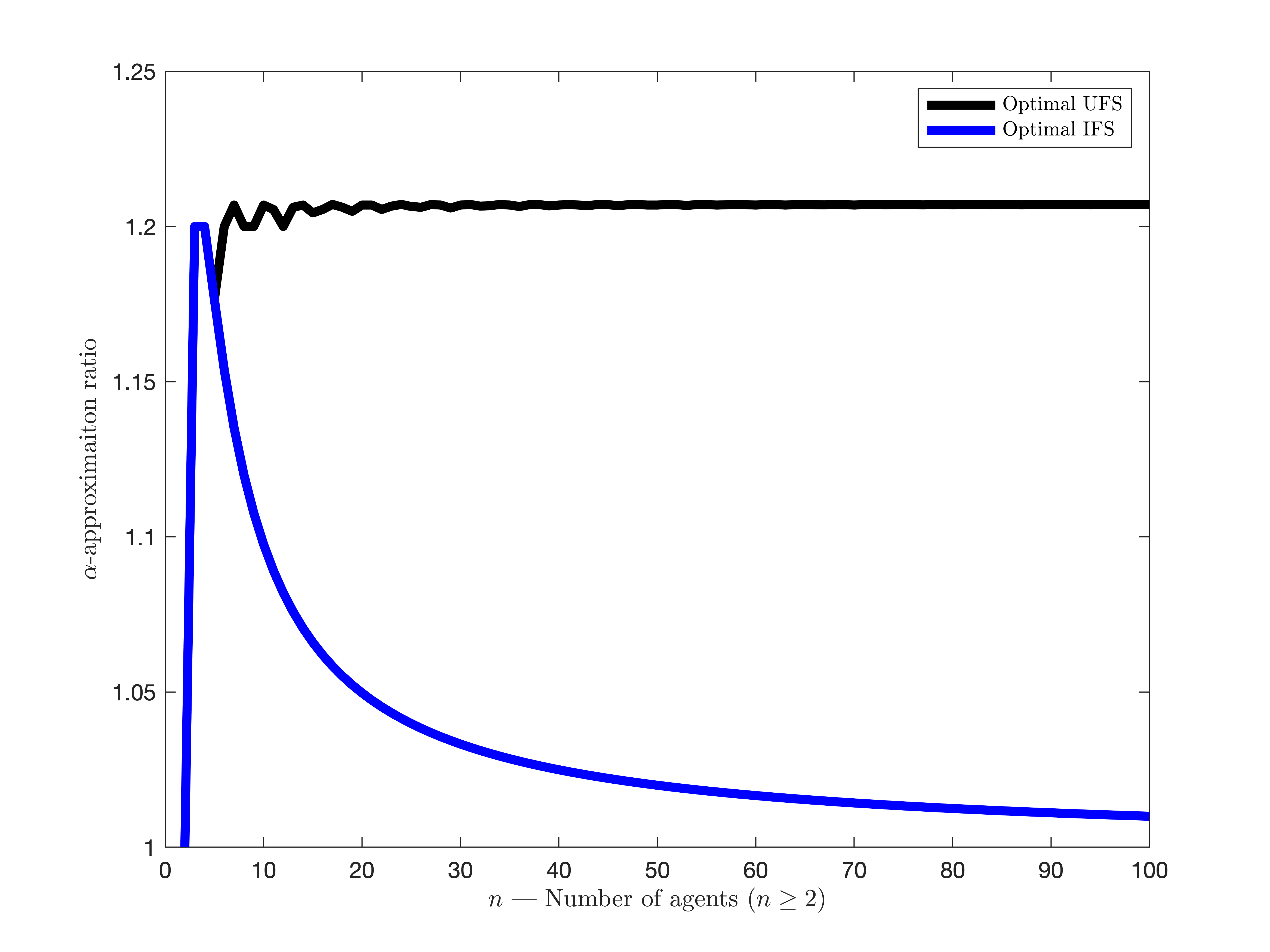
We now proceed to our analysis. Lemma 1 provides a welfare approximation lower bound for mechanisms that satisfy IFS.

Lemma 1.

Any mechanism satisfying IFS has a welfare approximation of at least $1+\frac{n-2}{n^{2}-2n+2}$ . As $n\rightarrow\infty$ , this lower bound approaches $1$ .

We now provide an example of an IFS mechanism, which we call the Constrained Median mechanism, that obtains the welfare approximation of Lemma 1. The Constrained Median mechanism locates the facility at the median location whenever the median location lies in the interval $[L/n,L(1-1/n)]$ . When the median location is below $L/n$ (resp., above $L(1-1/n)$ ), the facility is located at the minimum of $L/n$ and maximum-agent report (resp., maximum of $L(1-1/n)$ and the minimum-agent report). Definition 11 provides a formal definition, and Figure 2 provides an illustration of the mechanism.

Definition 11 (Constrained Median).

The Constrained Median mechanism $f_{\text{CM}}$ is a phantom mechanism that places $\lceil\frac{n-1}{2}\rceil$ phantoms at $L/n$ and the remaining phantoms at $L(1-\frac{1}{n})$ .

Theorem 4 says that the Constrained Median mechanism obtains the best welfare approximation guarantee among all IFS mechanisms, including non-strategyproof mechanisms. Furthermore, the Constrained Median mechanism can easily be seen to not only satisfy IFS but also to be strategyproof, anonymous, and unanimous (Theorem 1).

Theorem 4.

Among all IFS mechanisms, the Constrained Median mechanism provides the best welfare approximation guarantee, i.e., it achieves the approximation ratio in Lemma 1.

The intuition behind the welfare approximation ratio converging to $1$ is that as $n$ approaches infinity, the phantoms placed at $L/n$ (and $L(1-1/n)$ ) converge to $0$ (and $L$ ), and hence the Constrained mechanism mechanism converges to the median mechanism.

Lemma 2 provides a minimum welfare approximation bound for mechanisms that satisfy UFS (or proportionality or PF).

Lemma 2.

Any mechanism satisfying UFS (or proportionality or PF) has a welfare approximation of at least

\displaystyle\max_{k\in\mathbb{N}\ :\ 0\leq k\leq n/2}\frac{n(n-k)}{k^{2}+(n-k)^{2}}.

(6)

As $n\rightarrow\infty$ , this lower bound approaches $\frac{\sqrt{2}+1}{2}\approx 1.207$ .

We now show that the Uniform Phantom mechanism obtains the welfare approximation of Lemma 2. This means that the Uniform Phantom mechanism provides the best welfare approximation guarantee among all UFS (or proportional or PF) mechanisms, including non-strategyproof mechanisms. Furthermore, from Theorem 2, we know that the Uniform Phantom mechanism has the added benefit of being strategyproof, anonymous, and unanimous.

Theorem 5.

Among all UFS (or proportional or PF) mechanisms, the Uniform Phantom mechanism provides the best welfare approximation guarantee, i.e., it achieves the approximation ratio in Lemma 2.

Figure 3 illustrates the approximation results of this section.

7 Discussion and directions for future research.

Facility location is a classical problem in economic design. In this paper, we provided a deeper understanding of strategyproof and proportionally fair mechanisms. Table 1 provides an overview of most of the mechanisms considered in the paper and the properties they satisfy. Our results provide strong support for the desirability of the Uniform Phantom mechanism in terms of satisfying fairness and strategyproofness.

Table 1: Summary of results. All mechanisms are also unanimous, anonymous and Pareto efficient. Proofs of the results for the Average mechanism can be found in Appendix B. The welfare approximation results for the Nash and Midpoint mechanisms are from Lam et al. 2021, and the total cost approximation results for those mechanisms can be found in Appendix C.

Mechanism	Strategyproof	PF	UFS	Proportionality	IFS	Util-approx (limit)	Cost-approx
Uniform Phantom	Yes	Yes	Yes	Yes	Yes	$\frac{\sqrt{2}+1}{2}\approx 1.207$	$n-1$
Median	Yes	No	No	No	No	$1$	$1$
Constrained Median	Yes	No	No	No	Yes	$1$	$n-1$
Nash mechanism	No	Yes	Yes	Yes	Yes	$\in[\frac{\sqrt{2}+1}{2},2]$	$\in[2-\frac{2}{n},\frac{n}{2}]$
Midpoint mechanism	No	No	No	No	Yes	$2$	$\frac{n}{2}$
Average mechanism	No	Yes	Yes	Yes	Yes	$\frac{\sqrt{2}+1}{2}$	$2-\frac{2}{n}$

Moving beyond the fairness axioms that we presented, one can also consider stronger notions of proportionality-based fairness. For example, the following property, which we call Strong Proportional Fairness (SPF), is stronger than PF. Given a profile of locations $\boldsymbol{x}$ within range of distance $R$ , a facility location $y$ satisfies Strong Proportional Fairness (SPF) if, for any subset of voters $S\subseteq N$ within a range of distance $r$ , the location should be at most $R\frac{n-|S|}{n}+r$ distance from each agent in $S$ , i.e., $d(y,x_{i})\leq R\frac{n-|S|}{n}+r$ for all $i\in S$ .

However, it can be easily shown that the Uniform Phantom mechanism does not satisfy SPF. Our result (that the Uniform Phantom mechanism is the only SP and PF mechanism) then implies that there exists no strategyproof and SPF mechanism. In this sense, the compatibility between strategyproofness and fairness axioms ceases to hold when we move from PF to SPF.

There are several directions for future work to build on the framework and results that we have presented. For example, it may be fruitful to extend our analysis to incorporate a facility with capacity constraints, multiple facilities, alternative fairness concepts, considering weaker notions of strategyproofness, or alternative utility functions that are not necessarily single-peaked. Considering alternative utility functions can implicitly allow for behavioral assumptions in how agents use or benefit from the facility. For example, if agents do not benefit at all from the facility location when it is beyond a threshold distance from their ideal location, then this would correspond to a utility function that it is single-peaked but, beyond a certain threshold distance from their peak location, the utility function becomes constant and takes its minimal value (Zhou et al. 2023, see, e.g.,). An important direction is also to extend the strategyproof and proportionally fair facility location problem to multiple dimensions. Although some real-world problems (such as the provision of public goods) are well-suited to a unidimensional setting, other real-world problems are better suited to a multidimensional setting. By leveraging existing strategyproofness results for the multidimensional facility location problem (such as Theorem 1 in Border and Jordan 1983, which applies to settings where agents have separable preferences) and developing appropriate multidimensional generalizations of the proportionality-based fairness axioms that we presented, we believe progress can be made on this.

References

(1)
Anastasiadis and Deligkas (2018) Anastasiadis, Eleftherios and Argyrios Deligkas, “Heterogeneous Facility Location Games,” in “International Conference on Autonomous Agents and Multiagent Systems (AAMAS 2018)” 2018, pp. 623–631.
Arrow et al. (2010) Arrow, Kenneth J., Amartya Sen, and Kotaro Suzumura, Handbook of social choice and welfare, Vol. 2, Elsevier, 2010.
Aziz and Lee (2020) Aziz, Haris and Barton E. Lee, “The expanding approvals rule: improving proportional representation and monotonicity,” Social Choice and Welfare, 2020, 54 (1), 1–45.
Aziz and Lee (2022) Aziz, Haris and Barton E Lee, “A characterization of proportionally representative committees,” Games and Economic Behavior, 2022, 133, 248–255.
Aziz et al. (2019a) Aziz, Haris, Anna Bogomolnaia, and Hervé Moulin, “Fair mixing: the case of dichotomous preferences,” in “Proceedings of the 2019 ACM Conference on Economics and Computation” 2019, pp. 753–781.
Aziz et al. (2019b) Aziz, Haris, Felix Brandt, Edith Elkind, and Piotr Skowron, “Computational social choice: The first ten years and beyond,” in “Computing and software science,” Springer, 2019, pp. 48–65.
Aziz et al. (2020a) Aziz, Haris, Hau Chan, Barton E. Lee, and David C. Parkes, “The capacity constrained facility location problem,” Games and Economic Behavior, 2020, 124, 478–490.
Aziz et al. (2020b) Aziz, Haris, Hau Chan, Barton E. Lee, Bo Li, and Toby Walsh, “Facility location problem with capacity constraints: Algorithmic and mechanism design perspectives,” in “Proceedings of the AAAI Conference on Artificial Intelligence,” Vol. 34 2020, pp. 1806–1813.
Aziz et al. (2017) Aziz, Haris, Markus Brill, Vincent Conitzer, Edith Elkind, Rupert Freeman, and Toby Walsh, “Justified Representation in Approval-Based Committee Voting,” Social Choice and Welfare, 2017, pp. 461–485.
Barberà and Nicolò (2021) Barberà, Salvador and Antonio Nicolò, “Information disclosure with many alternatives,” Social Choice and Welfare, 2021, pp. 1–23.
Barberà and Jackson (1994) Barberà, Salvador and Matthew Jackson, “A characterization of strategy-proof social choice functions for economies with pure public goods,” Social Choice and Welfare, 1994, 11 (3), 241–252.
Barberà et al. (1998) Barberà, Salvador, Jordi Massó, and Shigehiro Serizawa, “Strategy-proof voting on compact ranges,” Games and Economic Behavior, 1998, 25, 272–291.
Bigman and Fofack (2000) Bigman, David and Hippolyte Fofack, “Spatial indicators of access and fairness for the location of public facilities,” Geographical targeting for poverty alleviation: methodology and applications. The World Bank, Washington, DC, 2000, pp. 181–206.
Bogomolnaia et al. (2005) Bogomolnaia, Anna, Hervé Moulin, and Richard Stong, “Collective choice under dichotomous preferences,” Journal of Economic Theory, 2005, 122 (2), 165–184.
Border and Jordan (1983) Border, Kim C. and James S. Jordan, “Straightforward Elections, Unanimity and Phantom Voters,” Review of Economic Studies, 1983, 50 (1), 153–170.
Brandeau and Chiu (1989) Brandeau, Margaret L. and Samuel S. Chiu, “An overview of representative problems in location research,” Management Science, 1989, 35 (6), 645–674.
Cantala (2004) Cantala, David, “Choosing the level of a public good when agents have an outside option,” Social Choice and Welfare, 2004, 22 (3), 491–514.
Caragiannis et al. (2022) Caragiannis, Ioannis, George Christodoulou, and Nicos Protopapas, “Truthful aggregation of budget proposals with proportionality guarantees,” in “Proceedings of the 36th AAAI Conference on Artificial Intelligence (AAAI)” 2022, p. 17.
Chan et al. (2021) Chan, Hau, Aris Filos-Ratsikas, Bo Li, Minming Li, and Chenhao Wang, “Mechanism Design for Facility Location Problems: A Survey,” in “Proceedings of the 30th International Joint Conference on Artificial Intelligence (IJCAI)” 2021.
Ching (1997) Ching, Stephen, “Strategy-proofness and “Median Voters”,” International Journal of Game Theory, 1997, 26, 473–490.
Debreu (1952) Debreu, Gerard, “A social equilibrium existence theorem,” Proceedings of the National Academy of Sciences, 1952, 38 (10), 886–893.
Deligkas et al. (2023) Deligkas, Argyrios, Aris Filos-Ratsikas, and Alexandros A Voudouris, “Heterogeneous facility location with limited resources,” Games and Economic Behavior, 2023, 139, 200–215.
Dragu and Laver (2019) Dragu, Tiberiu and Michael Laver, “Coalition governance with incomplete information,” Journal of Politics, 2019, 81 (3), 923–936.
Dummett (1984) Dummett, Michael, Voting Procedures, Oxford University Press, 1984.
Dummett (1997) Dummett, Michael, Principles of Electoral Reform, Oxford University Press, 1997.
Ehlers (2002) Ehlers, Lars, “Multiple Public Goods and Lexicographic Preferences,” Journal of Mathematical Economics, 2002, 37 (1), 1–14.
Ehlers (2003) Ehlers, Lars, “Multiple Public Goods and Lexicographic Preferences and Single-Plateaued Preference Rules,” Games and Economic Behavior, 2003, 43 (1), 1–27.
Endriss (2017) Endriss, Ulle, Trends in computational social choice, Lulu. com, 2017.
Faliszewski et al. (2017) Faliszewski, Piotr, Piotr Skowron, Arkadii Slinko, and Nimrod Talmon, “Multiwinner Voting: A New Challenge for Social Choice Theory,” in U. Endriss, ed., Trends in Computational Social Choice, 2017, chapter 2. Forthcoming.
Fan (1952) Fan, Ky, “Fixed-point and minimax theorems in locally convex topological linear spaces,” Proceedings of the National Academy of Sciences of the United States of America, 1952, 38 (2), 121.
Feldman et al. (2016) Feldman, Michal, Amos Fiat, and Iddan Golomb, “On voting and facility location,” in “Proceedings of the 17th ACM Conference on Electronic Commerce (ACM-EC)” 2016, pp. 269–286.
Freeman et al. (2021) Freeman, Rupert, David M. Pennock, Dominik Peters, and Jennifer Wortman Vaughan, “Truthful aggregation of budget proposals,” Journal of Economic Theory, 2021, 193, 105234.
Gibbard (1973) Gibbard, Allan, “Manipulation of voting schemes: A general result,” Econometrica, 1973, 41 (4), 587–601.
Glicksberg (1952) Glicksberg, Irving L., “A further generalization of the Kakutani fixed point theorem, with application to Nash equilibrium points,” Proceedings of the American Mathematical Society, 1952, 3 (1), 170–174.
Jackson and Nicolò (2004) Jackson, Matthew O. and Antonio Nicolò, “The strategy-proof provision of public goods under congestion and crowding preferences,” Journal of Economic Theory, 2004, 115, 278–308.
Jennings et al. (2021) Jennings, Andrew, Rida Laraki, Clemens Puppe, and Estelle Varloot, “New Characterizations of Strategy-Proofness under Single-Peakedness,” arXiv preprint arXiv:2102.11686, 2021.
Jung et al. (2020) Jung, Christopher, Sampath Kannan, and Neil Lutz, “Service in your neighborhood: Fairness in center location,” Foundations of Responsible Computing (FORC), 2020.
Klamler (2010) Klamler, Christian, “Fair division,” in “Handbook of group decision and negotiation,” Springer, 2010, pp. 183–202.
Klaus et al. (1998) Klaus, Bettina, Hans Peters, and Ton Storcken, “Strategy-proof division with single-peaked preferences and individual endowments,” Social Choice and Welfare, 1998, 15, 297–311.
Kurz et al. (2017) Kurz, Sascha, Nicola Maaser, and Stefan Napel, “On the democratic weights of nations,” Journal of Political Economy, 2017, 125 (5), 1599–1634.
Laffond (1980) Laffond, Gilbert, “Revelations Des Preferences et Utilités Unimodles,” Working Paper: Laboratoire d’Econometrie du CNAM, 1980.
Lam et al. (2021) Lam, Alexander, Haris Aziz, and Toby Walsh, “Nash Welfare and Facility Location,” The 8th International Workshop on Computational Social Choice (COMSOC-2021). (latest version: arXiv preprint arXiv:2310.04102), 2021.
Laslier and Sanver (2010) Laslier, Jean-François and M Remzi Sanver, Handbook on approval voting, Springer Science & Business Media, 2010.
Massó and Moreno De Barreda (2011) Massó, Jordi and Inés Moreno De Barreda, “On strategy-proofness and symmetric single-peakedness,” Games and Economic Behavior, 2011, 72 (2), 467 –484.
Mill (1861) Mill, John Stuart, Considerations on representative government 1861.
Miyagawa (1998) Miyagawa, Eiichi, “Mechanisms for providing a menu of public goods,” PhD dissertation, University of Rochester, 1998.
Miyagawa (2001) Miyagawa, Eiichi, “Locating libraries on a street,” Social Choice and Welfare, 2001, 18, 527–541.
Moulin (1980) Moulin, Hervé, “On Strategy-proofness and single peakedness,” Public Choice, 1980, 45 (4), 437–455.
Moulin (2003) Moulin, Hervé, Fair division and collective welfare, MIT press, 2003.
Moulin (2017) Moulin, Hervé, “One-dimensional mechanism design,” Theoretical Economics, 2017, 12 (2), 587–619.
Mulligan (1991) Mulligan, Gordon, “Equality measures and facility location,” Papers in Regional Science, 1991, 70 (4), 345–365.
Nash (1950) Nash, John, “The Bargaining Problem,” Econometrica, 1950, 18 (2), 155–162.
Nash (1953) Nash, John, “Two-Person Cooperative Games,” Econometrica, 1953, 21 (1), 128–140.
Nehring and Puppe (2006) Nehring, Klaus and Clemens Puppe, “The structure of strategy-proof social choice — Part I: General characterization and possibility results on median spaces,” Journal of Economic Theory, 2006, 135 (1), 269–305.
Nehring and Puppe (2007) Nehring, Klaus and Clemens Puppe, “Efficient and strategy-proof voting rules: A characterization,” Games and Economic Behavior, 2007, 59 (1), 132–153.
Nisan and Ronen (2001) Nisan, N. and A. Ronen, “Algorithmic Mechanism Design,” Games and Economic Behavior, 2001, 35 (1), 166–196.
Ozdaglar (2010) Ozdaglar, Asu, “Lecture 5: Existence of a Nash equilibrium from (6.254),” in “Game theory with engineering applications,” MIT OpenCourseWare Lecture notes, Spring, 2010.
Peremans et al. (1997) Peremans, W., H. Peters, H. v.d. Stel, and T. Storcken, “Strategy-proofness on Euclidean spaces,” Social Choice and Welfare, 1997, 14, 379–401.
Peters et al. (1992) Peters, Hans, Hans van der Stel, and Ton Storcken, “Pareto optimality, anonymity, and strategy-proofness in location problems,” International Journal of Game Theory, 1992, 21, 221–235.
Procaccia and Tennenholtz (2013) Procaccia, Ariel D. and Moshe Tennenholtz, “Approximate Mechanism Design Without Money,” in “Proceedings of the 14th ACM Conference on Electronic Commerce (ACM-EC)” ACM Press 2013, pp. 1–26.
Rawls (1971) Rawls, John, A Theory of Justice, Harvard University Press, 1971.
Renault and Trannoy (2005) Renault, Régis and Alain Trannoy, “Protecting Minorities through the Average Voting Rule,” Journal of Public Economic Theory, 2005, 7 (2), 169–199.
Renault and Trannoy (2011) Renault, Régis and Alain Trannoy, “Assessing the extent of strategic manipulation: the average vote example,” SERIEs, 2011, 2 (4), 497–513.
Sánchez-Fernández et al. (2017) Sánchez-Fernández, Luis, Edith Elkind, Martin Lackner, Norberto Fernández, Jesús Fisteus, Pablo Basanta Val, and Piotr Skowron, “Proportional justified representation,” in “Proceedings of the AAAI Conference on Artificial Intelligence,” Vol. 31 2017.
Satterthwaite (1975) Satterthwaite, Mark Allen, “Strategy-proofness and Arrow’s conditions: Existence and correspondence theorems for voting procedures and social welfare functions,” Journal of Economic Theory, 1975, 10, 187–217.
Scarf (1967) Scarf, Herbert E, “The core of an N person game,” Econometrica, 1967, pp. 50–69.
Schummer and Vohra (2002) Schummer, James and Rakesh V. Vohra, “Strategy-proof Location on a Network,” Journal of Economic Theory, 2002, 104, 405–428.
Sen (1980) Sen, Amartya, “Equality of what?,” The Tanner lecture on human values, 1980, 1, 197–220.
Shapley (1953) Shapley, Lloyd S., A Value for $n$ -Person Games, Princeton, NJ: Princeton University Press,
Sprumont (1991) Sprumont, Yves, “The division problem with single-peaked preferences: a characterization of the uniform allocation rule,” Econometrica: Journal of the Econometric Society, 1991, pp. 509–519.
Steinhaus (1948) Steinhaus, Hugo, “The problem of fair division,” Econometrica, 1948, 16, 101–104.
Weymark (2008) Weymark, John A, “Strategy-Proofness and the Tops-Only Property,” Journal of Public Economic Theory, 2008, 10 (1), 7–26.
Weymark (2011) Weymark, John A., “A unified approach to strategy-proofness for single-peaked preferences,” SERIEs, 2011, 2 (4), 529–550.
Yaari (1981) Yaari, Menahem E, “Rawls, Edgeworth, Shapley, Nash: Theories of distributive justice re-examined,” Journal of Economic Theory, 1981, 24 (1), 1–39.
Yamamura and Kawasaki (2013) Yamamura, Hirofumi and Ryo Kawasaki, “Generalized average rules as stable Nash mechanisms to implement generalized median rules,” Social Choice and Welfare, March 2013, 40 (3), 815–832.
Zanjirani Farahani and Hekmatfar (2009) Zanjirani Farahani, Reza and Masoud Hekmatfar, Facility location: concepts, models, algorithms and case studies, Springer Science & Business Media, 2009.
Zhou et al. (2023) Zhou, Houyu, Guochuan Zhang, Lili Mei, and Minming Li, “Facility Location Games with Thresholds,” in “Proceedings of the 2023 International Conference on Autonomous Agents and Multiagent Systems” 2023, pp. 2170–2178.
Zhou et al. (2022) Zhou, Houyu, Minming Li, and Hau Chan, “Strategyproof Mechanisms for Group-Fair Facility Location Problems,” in “Proceedings of the Thirty-First International Joint Conference on Artificial Intelligence” 2022, pp. 613–619.
Zou and Li (2015) Zou, Shaokun and Minming Li, “Facility location games with dual preference,” in “Proceedings of the 2015 international conference on autonomous agents and multiagent systems” 2015, pp. 615–623.

Appendix A Omitted proofs.

A.1 Proof of Proposition 1.

Proof.

Point (i): We wish to prove that UFS implies proportionality, IFS, and unanimity. Let $\boldsymbol{x}$ be an arbitrary location profile and let $y$ be a facility location that satisfies UFS. From the definition of UFS, it is immediate that IFS and unanimity are satisfied. It remains to prove that proportionality is satisfied. For the sake of a contradiction, suppose that proportionality is not satisfied. That is, $\boldsymbol{x}$ is such that $x_{i}\in\{0,L\}$ for all $i\in N$ and $y\neq L\frac{|i\in N\ :\ x_{i}=1|}{n}$ . Let $k=|i\in N\ :\ x_{i}=L|$ . If $k=0$ , then UFS requires that $y=0$ , and proportionality is satisfied—a contradiction. If $k>0$ , then UFS requires that:

|L-y|\leq L(1-\frac{k}{n}),\quad\text{i.e.,}\quad y\geq\frac{kL}{n}\qquad\text{and}\qquad|0-y|\leq L(1-\frac{n-k}{n}),\quad\text{i.e.,}\quad y\leq\frac{kL}{n}.

The inequalities above imply that $y=\frac{kL}{n}$ and proportionality is satisfied—a contradiction.

Point (ii): We wish to prove that PF implies UFS. This follows immediately by noting that a set of agents all located at the same location are within a range of distance $r=0$ . Taking $r=0$ in the PF definition shows that PF implies UFS.

It is straightforward to see that the relations in the proposition are strict and also that there is no logical relation between proportionality, IFS, and unanimity. We omit the proofs. ∎

A.2 Proof of Proposition 2.

Proof.

Point (i): We wish to prove that the median mechanism satisfies unanimity and strategyproofness, but does not satisfy IFS, PF, UFS, nor Proportionality. The median mechanism is known to be strategyproof (Procaccia and Tennenholtz 2013); it is also clearly unanimous. Finally, consider the agent location profile with $n-1$ agents at $0$ and $1$ agent at $L$ . The median mechanism locates the facility at $0$ , which violates both IFS and Proportionality (and hence also UFS and PF).

Point (ii): We wish to prove that the midpoint mechanism satisfies IFS and unanimity, but does not satisfy strategyproofness, PF, UFS, nor Proportionality. The midpoint mechanism places the facility at the average of the leftmost and rightmost agent. It is therefore unanimous but not strategyproof. The maximum cost that can be incurred by an agent is $L/2$ , which is obtained when the leftmost agent is at $0$ and the rightmost agent is at $L$ . However, this IFS is satisfied since $n\geq 2$ . To see that the midpoint mechanism does not satisfy Proportionality, consider the agent location profile with 2 agents at $0$ and 1 agent at $L$ . The midpoint mechanism places the facility at $L/2$ , but Proportionality requires that the mechanism is placed at $L/3$ . Since Proportionality is not satisfied, UFS and PF are also not satisfied.

Point (iii): We wish to prove that the Nash mechanism satisfies PF but is not strategyproof. To this end, we first define a notion of monotonicity that requires that if a location profile is modified by an agent shifting its location, the facility placement under the modified profile will not shift in the opposite direction. Definition 12 formalizes this notion.

Definition 12 (Monotonic).

A mechanism $f$ is monotonic if

f(\boldsymbol{x})\leq f(\boldsymbol{x}^{\prime})

for all $f(\boldsymbol{x})$ and $f(\boldsymbol{x}^{\prime})$ such that $x_{i}\leq x_{i}^{\prime}$ for all $i\in N$ and $x_{i}<x_{i}^{\prime}$ for some $i\in N$ .

We next prove the following auxiliary lemma.

Lemma 3.

A mechanism that satisfies UFS and monotonicity also satisfies PF.

Proof.

Let $\boldsymbol{x}$ be an arbitrary agent location profile, and $f$ be a mechanism that satisfies UFS and monotonicity. Consider the set $S=\{1,\dots,m\}\subset N$ of $m$ agents and denote $r:=\max_{i\in S}\{x_{i}\}-\min_{i\in S}\{x_{i}\}$ . We prove that the maximum distance of the facility from any agent in $S$ is at most $L\frac{n-m}{n}+r$ .

Denote $f:=\argmax_{i\in S}\{d(f(\boldsymbol{x}),x_{i})\}$ as the agent in $S$ whose location $x_{f}$ under $\boldsymbol{x}$ is furthest from the respective facility location, which is either $\max_{i\in S}\{x_{i}\}$ or $\min_{i\in S}\{x_{i}\}$ . Consider the modified profile $\boldsymbol{x}^{\prime}$ where $x_{i}^{\prime}=\max_{i\in S}\{x_{i}\}$ for all $i\in S$ if $f(\boldsymbol{x})\geq x_{f}$ and $x_{i}^{\prime}=\min_{i\in S}\{x_{i}\}$ for all $i\in S$ if $f(\boldsymbol{x})<x_{f}$ . Also, $x_{i}^{\prime}=x_{i}$ for all $i\in N\backslash S$ . In other words, the agents in $S$ have their locations moved to the rightmost agent in $S$ if the facility is weakly right of the furthest agent of $S$ under $\boldsymbol{x}$ . If the facility is strictly left of the furthest agent of $S$ under $\boldsymbol{x}$ , the agents in $S$ have their locations moved to the leftmost agent.

Due to monotonicity, the facility does not move closer to $x_{f}$ when modifying $\boldsymbol{x}$ to $\boldsymbol{x}^{\prime}$ , so we have

d(f(\boldsymbol{x}^{\prime}),x_{f})\geq d(f(\boldsymbol{x}),x_{f}).

Note that all $m$ agents of $S$ are at the same location under $\boldsymbol{x}^{\prime}$ . Denote this location as $x_{S}^{\prime}$ . Due to UFS, we also have

d(f(\boldsymbol{x}^{\prime}),x_{S}^{\prime})\leq L\frac{n-m}{n}.

We therefore have

\displaystyle d(f(\boldsymbol{x}),x_{f})

\displaystyle\leq d(f(\boldsymbol{x}^{\prime}),x_{f})\leq d(f(\boldsymbol{x}^{\prime}),x_{S}^{\prime})+r\leq L\frac{n-m}{n}+r.

∎

The Nash mechanism is known to satisfy UFS and monotonicity (Lam et al. 2021). It therefore satisfies PF. ∎

A.3 Tightness of Theorem 1.

Proof.

We wish to prove that each of the requirements in Theorem 1 are necessary for the theorem to hold. We show that if any one of the requirements (i.e., strategyproofness, unanimity, anonymity, and IFS) are removed, then Theorem 1—not only fails to hold—but there exists such a mechanism. We do this by providing examples of mechanisms that fulfill all but one of the requirements of Theorem 1 but that are not phantom mechanisms with the $n-1$ phantoms contained in $[L/n,L(1-1/n)]$ .

Strategyproofness. By Proposition 2, the midpoint mechanism is an example of a mechanism that is not strategyproof, but satisfies unanimity, anonymity and IFS. However, the midpoint mechanism is not a phantom mechanism—this follows immediately because phantom mechanisms are necessarily strategyproof.

Unanimity. For $n\geq 2$ , consider the constant- $\frac{L}{2}$ mechanism, whereby the facility is always located at $\frac{L}{2}$ . This mechanism is clearly strategyproof and anonymous and does not satisfy unanimity. Furthermore, it satisfies IFS because the largest cost that any agent can experience is $\frac{L}{2}$ , which is (weakly) lower than $L(1-\frac{1}{n})$ for any $n\geq 2$ . However, the constant- $\frac{L}{2}$ mechanism is not a phantom mechanism—this follows immediately because phantom mechanisms necessarily satisfy unanimity.

Anonymity. For simplicity take $n=3$ and consider the mechanism $f$ that locates the facility at

	$\displaystyle f(\boldsymbol{x}):=$	$\displaystyle\max\{\min\{x_{1},\frac{L}{3}+\varepsilon\},\min\{x_{2},\frac{L}{3}\},\min\{x_{3},\frac{L}{3}\},$
		$\displaystyle\qquad\min\{x_{1},x_{2},L(1-\frac{1}{3})\},\min\{x_{2},x_{3},L(1-\frac{1}{3})\},\min\{x_{1},x_{3},L(1-\frac{1}{3})\},$
		$\displaystyle\qquad\min\{x_{1},x_{2},x_{3},L\},0\},$

where $\varepsilon>0$ is sufficiently small. This is a Generalized Median mechanism (Border and Jordan 1983) and, hence, is strategyproof. Furthermore, it is easy to see that $f$ is unanimous. Border and Jordan 1983’s (Border and Jordan 1983) Lemma 3 then says that $f$ is Pareto efficient. However, the mechanism is not anonymous: for $\boldsymbol{x}=(0,0,L)$ , $f(\boldsymbol{x})=L/3$ , but for $\boldsymbol{x}^{\prime}=(L,0,0)$ , $f(\boldsymbol{x}^{\prime})=L/3+\varepsilon$ .

We now show that the mechanism satisfies IFS. Since the mechanism is Pareto efficient, IFS is trivially satisfied if $x_{i}\leq L(1-\frac{1}{3})$ for all $i\in N$ or if $x_{i}\geq\frac{L}{3}$ for all $i\in N$ . Now consider some location profile $\boldsymbol{x}$ that does not belong to these trivial cases, i.e., there is at least one agent with location below $\frac{L}{3}$ (resp., $L(1-\frac{1}{3})$ ) and at least one agent with location above $\frac{L}{3}$ (resp., $L(1-\frac{1}{3})$ ). In these cases, IFS can only possibly be violated if $f(\boldsymbol{x})>L(1-\frac{1}{3})$ or $f(\boldsymbol{x})<\frac{L}{3}$ . However, $f(\boldsymbol{x})>L(1-\frac{1}{3})$ if and only if $x_{i}>L(1-\frac{1}{3})$ for all $i\in N$ —but the latter condition does not hold. Similarly, $f(\boldsymbol{x})<\frac{L}{3}$ if and only if $x_{i}<\frac{L}{3}$ for all $i\in N$ —but, again, the latter condition does not hold. Therefore, we conclude that IFS is satisfied. However, the mechanism $f$ is not a phantom mechanism—this follows immediately because phantom mechanisms are necessarily anonymous.

IFS.

The Phantom mechanism that places all $n-1$ phantoms at $0$ is strategyproof, unanimous and anonymous. However, it does not satisfy IFS as the facility can be placed at $0$ when there is an agent at $L$ . It is immediate that this Phantom mechanism violates the condition of the theorem that all phantoms are located in the interval $[L/n,L(1-1/n)]$ . ∎

A.4 Proof of Proposition 3.

Proof.

The Uniform Phantom mechanism is strategyproof since it is a Phantom mechanism and all Phantom mechanisms are strategyproof (Massó and Moreno De Barreda 2011, see, e.g., Corollary 2 of). We now prove that the Uniform Phantom mechanism satisfies PF. Let $\boldsymbol{x}$ be an arbitrary location profile and let $S=\{1,\dots,s\}\subseteq N$ be a set of $s$ agents; denote $r:=\max_{i\in S}\{x_{i}\}-\min_{i\in S}\{x_{i}\}$ . We prove $d(f(\boldsymbol{x}),x_{i})\leq L\frac{n-s}{n}+r$ for all $i\in S$ . If $r=L$ , then the result is trivially true. Suppose that $r<L$ . If the location is within the range of the agents in $S$ , PF is immediately satisfied. Next we consider the case there the location is outside the range of the agents in $S$ . Recall that the Uniform Phantom mechanism places the facility at the $n$ -th entity of the $2n-1$ phantoms and agents. There are at least $s$ agents in the range of the locations of the agents in $S$ , so the facility is at most $n-s$ phantoms away from the nearest agent in $S$ . Since the distance between adjacent phantoms is $L/n$ , the facility is at most distance $(n-s)L/n$ from the nearest agent in $S$ . Hence, the maximum distance of the facility from any agent in $S$ is $L\frac{n-s}{n}+r$ . ∎

A.5 Lemma 4 and proof of Lemma 4.

Lemma 4.

A mechanism that is strategyproof, unanimous, and proportional must also be anonymous.

Proof.

Suppose $f$ is strategyproof and satisfies proportionality and unanimity. We wish to show that $f$ is anonymous (Definition 1). First we note that by Border and Jordan 1983’s (Border and Jordan 1983) Proposition 2, any unanimous and strategyproof mechanism must satisfy the following uncompromising property.

Definition 13 (Uncompromising).

A mechanism $f$ is uncompromising if, for every profile of locations $\boldsymbol{x}$ , and each agent $i\in N$ , if $f(\boldsymbol{x})=y$ then

	$\displaystyle x_{i}>y$	$\displaystyle\implies f(x_{i}^{\prime},\boldsymbol{x}_{-i})=y\qquad\text{ for all }x_{i}^{\prime}\geq y$		and,		(7)
	$\displaystyle x_{i}<y$	$\displaystyle\implies f(x_{i}^{\prime},\boldsymbol{x}_{-i})=y\qquad\text{ for all }x_{i}^{\prime}\leq y.$				(8)

Now consider an arbitrary profile of locations $\boldsymbol{x}$ and an arbitrary permutation of the profile $\boldsymbol{x}$ , which we denote by $\boldsymbol{x}_{\sigma}$ . We will show that $f(\boldsymbol{x})=f(\boldsymbol{x}_{\sigma})$ . First note that if $\boldsymbol{x}$ is such that $x_{i}=c$ for some $c\in[0,L]$ , then $f(\boldsymbol{x})=f(\boldsymbol{x}_{\sigma})$ by unanimity. Therefore, we assume that $\boldsymbol{x}$ is such that $x_{i}\neq x_{j}$ for some $i,j\in N$ .

Case 1.

Suppose that $f(\boldsymbol{x})\neq x_{i}$ for any $i\in N$ . Recall that Border and Jordan 1983’s (Border and Jordan 1983) Lemma 3 says that any strategyproof and unanimous mechanism is Pareto efficient; therefore, $\min_{i\in N}x_{i}\leq f(\boldsymbol{x})\leq\max_{i\in N}x_{i}$ . Now if all agents strictly below (resp., above) $f(\boldsymbol{x})$ shift their location to $0$ (resp., $L$ ), then, by the uncompromising property, the facility location must be unchanged. Let $\boldsymbol{x}^{\prime}$ denote this augmented location profile and let $k^{\prime}$ denote the number of agents with $x_{i}^{\prime}=L$ . By proportionality, it must be that $f(\boldsymbol{x})=f(\boldsymbol{x}^{\prime})=\frac{k^{\prime}L}{n}$ . Now consider the permutation of the profile $\boldsymbol{x}^{\prime}$ , i.e., $\boldsymbol{x}_{\sigma}^{\prime}$ . The implication of the proportionality property is independent of agent labels; therefore, $f(\boldsymbol{x}_{\sigma}^{\prime})=f(\boldsymbol{x}^{\prime})$ . Now shift the agent locations in $\boldsymbol{x}_{\sigma}^{\prime}$ so that they replicate the permuted location profile $\boldsymbol{x}_{\sigma}$ —note that this process only involves agents strictly above (resp., below) $f(\boldsymbol{x}_{\sigma}^{\prime})$ moving to a location above (resp., below) $f(\boldsymbol{x}_{\sigma}^{\prime})$ . Therefore, by the uncompromising property, it must be that $f(\boldsymbol{x}_{\sigma}^{\prime})=f(\boldsymbol{x}_{\sigma})$ . Combining the three sets of equalities gives

f(\boldsymbol{x})=f(\boldsymbol{x}^{\prime})=f(\boldsymbol{x}_{\sigma}^{\prime})=f(\boldsymbol{x}_{\sigma}).

That is, the facility location is unchanged by permutations, i.e., anonymity is satisfied.

Case 2.

Suppose that $f(\boldsymbol{x})=x_{i}$ for some $i\in N$ . Let $M\subseteq N$ be the subset of agents with $x_{i}=f(\boldsymbol{x})$ . Let $M_{0},M_{1}\subseteq N$ correspond to the subset of agents with location strictly below and strictly above $f(\boldsymbol{x})$ , respectively. Denote $|M_{0}|=k_{0}$ and $|M_{1}|=k_{1}$ . We first show that

\displaystyle\frac{k_{1}L}{n}\leq f(\boldsymbol{x}).

(9)

For the sake of contradiction, suppose that (9) does not hold (i.e., $f(\boldsymbol{x})<\frac{k_{1}L}{n}$ ), and consider the location profile $\boldsymbol{x}^{\prime}$ obtained by modifying $\boldsymbol{x}$ such that the $M_{0}$ (resp., $M_{1}$ ) agents’ locations are shifted to $0$ (resp., $L$ ) and the other agents’ (i.e., those in $M$ ) have location unchanged. By the uncompromising property, $f(\boldsymbol{x}^{\prime})=f(\boldsymbol{x})$ . Now consider the modified location profile $\boldsymbol{x}^{\prime\prime}$ such that $x_{i}^{\prime\prime}=x_{i}^{\prime}$ for all $i\notin M$ and $x_{i}^{\prime\prime}=0$ for all $i\in M$ . By proportionality, $f(\boldsymbol{x}^{\prime\prime})=\frac{k_{1}L}{n}$ and, by supposition that $f(\boldsymbol{x})<\frac{k_{1}L}{n}$ , we have

\displaystyle f(\boldsymbol{x}^{\prime})=f(\boldsymbol{x})<\frac{k_{1}L}{n}=f(\boldsymbol{x}^{\prime\prime}).

(10)

Now notice that the profile $\boldsymbol{x}^{\prime}$ can be obtained from $\boldsymbol{x}^{\prime\prime}$ by shifting the subset of $M$ agents’ locations from $0$ to $f(\boldsymbol{x})$ , which is to the left of $f(\boldsymbol{x}^{\prime\prime})$ . The uncompromising property then requires that

f(\boldsymbol{x}^{\prime})=f(\boldsymbol{x}^{\prime\prime})=\frac{k_{1}L}{n},

which contradicts (10). We conclude that (9) holds.

With condition (9) in hand, we can now proceed by considering two subcases.

Subcase 2a.

Suppose that $f(\boldsymbol{x})=\frac{kL}{n}$ for some $k\in\{0,\ldots,n\}$ . Consider any profile of locations $\boldsymbol{x}^{\prime}\in\{0,L\}^{n}$ with $k$ agents at location $L$ . By proportionality, $f(\boldsymbol{x}^{\prime})=\frac{kL}{n}=f(\boldsymbol{x})$ . Note that the proportionality axiom is independent of agent labels and, by (9), $f(\boldsymbol{x})\geq\frac{k_{1}L}{n}\implies k\geq k_{1}$ . Therefore, the permuted location of profile $\boldsymbol{x}_{\sigma}$ can be attained by relabeling agents in $\boldsymbol{x}^{\prime}$ and then shifting their reports from $L$ (resp., $0$ ) to their original location that is weakly above (resp., below) $f(\boldsymbol{x}^{\prime})=\frac{kL}{n}$ —by the uncompromising property, the facility location will not change. Therefore, $f(\boldsymbol{x}_{\sigma})=f(\boldsymbol{x}^{\prime})=\frac{kL}{n}=f(\boldsymbol{x})$ , as required.

Subcase 2b.

Suppose that $f(\boldsymbol{x})\neq\frac{kL}{n}$ for any $k\in\{0,\ldots,n\}$ . Let $k^{*}$ be the smallest integer such that $f(\boldsymbol{x})<\frac{k^{*}L}{n}$ ; by (9), $k^{*}>k_{1}$ . Now consider any location profile $\boldsymbol{x}^{\prime}\in\{0,L\}^{n}$ with exactly $k^{*}$ agents at $L$ . By proportionality,

\displaystyle f(\boldsymbol{x}^{\prime})=\frac{k^{*}L}{n}>f(\boldsymbol{x}).

(11)

Now consider any subset $G\subseteq N$ that contains $|k^{*}-k_{1}|>1$ agents who are located at $L$ . Let $\boldsymbol{x}^{\prime\prime}$ denote the profile obtained from $\boldsymbol{x}^{\prime}$ by shifting the $G$ agents’ locations to $\hat{x}_{G}=f(\boldsymbol{x})$ . We shall prove that

\displaystyle f(\boldsymbol{x}^{\prime\prime})=\hat{x}_{G}.

(12)

To see this, suppose that this is not the case. Then either

	$\displaystyle\hat{x}_{G}$	$\displaystyle<f(\boldsymbol{x}^{\prime\prime})\qquad\text{or}$		(13)
	$\displaystyle f(\boldsymbol{x}^{\prime\prime})$	$\displaystyle<\hat{x}_{G}.$		(14)

In the former case, all agents in $G$ have location strictly below $f(\boldsymbol{x}^{\prime\prime})$ —namely, $\hat{x}_{G}=f(\boldsymbol{x})$ . Therefore, by the uncompromising property, if all agents in $G$ shift their location to $0$ in the profile $\boldsymbol{x}^{\prime\prime}$ , then the facility location is unchanged and continues to be located at $f(\boldsymbol{x}^{\prime\prime})$ . Proportionality then requires that the facility then be located at $\frac{k_{1}L}{n}$ and, hence, $f(\boldsymbol{x}^{\prime\prime})=\frac{k_{1}L}{n}$ . But then (13) implies that $\hat{x}_{G}<\frac{k_{1}L}{n}$ , which in turn implies that $f(\boldsymbol{x})=\hat{x}_{G}<\frac{k_{1}L}{n}$ —this contradicts (9). In the latter case, all agents in $G$ have location strictly above $f(\boldsymbol{x}^{\prime\prime})$ —namely, $\hat{x}_{G}=f(\boldsymbol{x})$ . Therefore, by the uncompromising property, if all agents in $G$ shift their location back to $L$ in the profile $\boldsymbol{x}^{\prime\prime}$ , then the facility location is unchanged and, by proportionality, is located at $\frac{k^{*}L}{n}$ . Hence, $f(\boldsymbol{x}^{\prime\prime})=\frac{k^{*}L}{n}$ . Using (14), this implies that $\frac{k^{*}L}{n}<f(\boldsymbol{x})$ , which contradicts (11).

Now given (12), by the uncompromising property, shifting any agent with location at 0 (resp., 1) to any location weakly below (resp., above) $\hat{x}_{G}$ must leave the facility’s location unchanged. Therefore, for any profile with exactly $k_{0},k_{1}$ agents strictly below $\hat{x}_{G}$ and strictly above $\hat{x}_{G}$ and $n-k_{0}-k_{1}$ agents located at $\hat{x}_{G}$ , the facility must be located at $\hat{x}_{G}$ . But—since $\hat{x}_{G}=f(\boldsymbol{x})$ —it is immediate that any permutation of $\boldsymbol{x}$ , say $\boldsymbol{x}_{\sigma}$ , satisfies these 3 properties; hence,

f(\boldsymbol{x}_{\sigma})=f(\boldsymbol{x}).

We conclude that any mechanism that satisfies strategyproofness, proportionality, unanimity must also satisfy anonymity. ∎

A.6 Unanimity is Necessary for Theorem 2.

Proof.

We wish to prove that Theorem 2 does not hold if unanimity is removed. It suffices to consider the following mechanism for $n=2$

f(\boldsymbol{x})=\begin{cases}0&\text{if $x_{1},x_{2}\leq L/4$,}\\ L&\text{if $x_{1},x_{2}\geq 3L/4$,}\\ L/2&\text{else.}\end{cases}

This mechanism is clearly anonymous, satisfies proportionality and is not the Uniform Phantom mechanism. It remains to show that it is strategyproof. Using a symmetry argument, we focus on deviations by agent 1 without loss of generality. Suppose $f(\boldsymbol{x})=0$ , then it must be that $x_{1}\leq L/4$ . But then agent 1 obtains the minimum possible distance to the facility (given $x_{1}$ and given the mechanism’s range); hence, no deviation can strictly decrease their distance. Suppose $f(\boldsymbol{x})=L/2$ , then either $x_{1}\in(L/4,3L/4)$ or $x_{2}\in(L/4,3L/4)$ . In the former case, agent 1 obtains the minimum possible distance to the facility (given $x_{1}$ and given the mechanism’s range); hence, no deviation can strictly decrease their distance. In the latter case, no deviation by agent 1 can change the facility location. Finally, suppose $f(\boldsymbol{x})=L$ , then it must be that $x_{1}\geq 3L/4$ . But then agent 1 obtains the minimum possible distance to the facility (given $x_{1}$ and given the mechanism’s range); hence, no deviation can strictly decrease their distance. Therefore, the mechanism is SP. ∎

A.7 Proof of Proposition 4.

Proof.

By Theorem 1, a strategyproof, anonymous, unanimous mechanism satisfies IFS must be a Phantom mechanism with $n-1$ phantoms all contained in the interval $[\frac{1}{n},L-\frac{1}{n}]$ . For such a Phantom mechanism, consider the location profile which places $n-1$ agents at $0$ and $1$ agent at the leftmost phantom $p_{1}$ . The Phantom mechanism places the facility at $p_{1}$ , leading to $(n-1)p_{1}$ total cost, and the optimal total cost is $p_{1}$ , achieved by placing the facility at $0$ . The total cost approximation ratio is therefore at least $n-1$ . Now, any Pareto optimal mechanism has a total cost approximation ratio of at most $n-1$ . To see this, note that for any agent location profile $\boldsymbol{x}$ where the distance between the leftmost and rightmost agents is $c$ , we must have $\Psi^{*}(\boldsymbol{x})\geq c$ , and $\Psi(f(\boldsymbol{x}))\leq(n-1)c$ . As a Phantom mechanism with $n-1$ phantoms is Pareto optimal, we see that a Phantom mechanism with $n-1$ phantoms all contained in the interval $[\frac{1}{n},L-\frac{1}{n}]$ has a total cost approximation ratio of $n-1$ , and thus the proposition statement follows. ∎

A.8 Proof of Lemma 1.

Proof.

We wish to prove that a mechanism $f$ that satisfies IFS has welfare approximation of at least $1+\frac{n-2}{n^{2}-2n+2}$ . To this end, suppose $f$ satisfies IFS and consider the profile of locations $\boldsymbol{x}\in\{0,L\}^{n}$ that places $n-1$ agents at $0$ . IFS requires that $f(\boldsymbol{x})\geq\frac{L}{n}$ (and $f(\boldsymbol{x})\leq L(1-\frac{1}{n})$ ), so any IFS mechanism has welfare of at most

\Phi(f(\boldsymbol{x}))\leq(n-1)L(1-\frac{1}{n})+\frac{L}{n}=\frac{L(n-1)^{2}+L}{n}.

However, for this instance, the welfare-optimal welfare is $\Phi^{*}(\boldsymbol{x})=L(n-1)$ (obtained by locating the facility at the median location, $0$ ). Therefore, the approximation ratio of $f$ is at least

\frac{\Phi^{*}(\boldsymbol{x})}{\Phi(f(\boldsymbol{x}))}=\frac{nL(n-1)}{L(n-1)^{2}+L}=1+\frac{n-2}{(n-1)^{2}+1}.

∎

A.9 Proof of Theorem 4.

Proof.

We wish to prove that among all IFS mechanisms, the Constrained Median mechanism provides the best welfare approximation guarantee i.e., it achieves the approximation ratio in Lemma 1. Let $f_{\text{CM}}$ denote the Constrained Median mechanism. We shall prove that for any location profile $\boldsymbol{x}\in[0,L]^{n}$ there exists some profile $\tilde{\boldsymbol{x}}\in\{0,L\}^{n}$ such that

\displaystyle\frac{\Phi^{*}(\tilde{\boldsymbol{x}})}{\Phi(f_{\text{CM}}(\tilde{\boldsymbol{x}}))}

\displaystyle\geq\frac{\Phi^{*}(\boldsymbol{x})}{\Phi(f_{\text{CM}}(\boldsymbol{x}))},

(15)

which implies that

\max_{\boldsymbol{x}\in[0,L]^{n}}\frac{\Phi^{*}(\boldsymbol{x})}{\Phi(f_{\text{CM}}(\boldsymbol{x}))}=\max_{\boldsymbol{x}\in\{0,L\}^{n}}\frac{\Phi^{*}(\boldsymbol{x})}{\Phi(f_{\text{CM}}(\boldsymbol{x}))}.

We begin by noting that, whenever $f_{\text{CM}}(\boldsymbol{x})\in(L/n,L(1-1/n))$ , the facility location coincides with the median location and $f_{\text{CM}}$ obtains the maximum welfare. Thus, we can restrict our attention to profiles such that $f_{\text{CM}}(\boldsymbol{x})\notin(L/n,L(1-1/n))$ . We proceed to prove (15) by considering a sequence of profiles that modify $\boldsymbol{x}$ into some profile $\tilde{\boldsymbol{x}}\in\{0,L\}^{n}$ such that each modified profile guarantees a weakly higher welfare approximation ratio.

Let the agent labels be ordered such that $x_{1}\leq\ldots\leq x_{n}$ ; let $i={med}$ denote the median agent. Without loss of generality, suppose $f_{\text{CM}}(\boldsymbol{x})\in[0,L/n]$ . This implies that the median agent is weakly below $f_{\text{CM}}(\boldsymbol{x})$ , i.e., $x_{med}\leq f_{\text{CM}}(\boldsymbol{x})$ . To assist with visualizing the proof technique, we provide a running example with $n=5$ agents. Figure 4 illustrates a profile $\boldsymbol{x}$ such that $x_{med}\leq f_{\text{CM}}(\boldsymbol{x})$ ; in particular, $x_{med}=x_{3}$ and $f_{\text{CM}}(\boldsymbol{x})=L/5$ .

Figure 4: Running example. Profile

\boldsymbol{x}

First, consider the modified profile $\boldsymbol{x}^{\prime}$ such that $x_{i}^{\prime}=0$ for $i\in N^{\prime}:=\{i\ :\ i<{med}\}$ and $x_{i}^{\prime}=x_{i}$ for all $i\notin N^{\prime}$ . Applying this operation to the running example illustrated in Figure 4, we obtain the profile illustrated in Figure 5.

Figure 5: Running example. Profile

\boldsymbol{x}^{\prime}

In this modified profile, we have moved all agents strictly left of the median agent to $0$ , so neither the welfare-optimal (median) location nor the facility location under $f_{\text{CM}}$ changes. Hence, relative to $\Phi^{*}(\boldsymbol{x})$ and $\Phi(f_{\text{CM}}(\boldsymbol{x}))$ , the optimal welfare, $\Phi^{*}(\boldsymbol{x}^{\prime})$ , and the welfare provided by $f_{\text{CM}}$ , $\Phi(f_{\text{CM}}(\boldsymbol{x}^{\prime}))$ , decrease by the same amount—namely, $\sum_{i\in N^{\prime}}x_{i}\geq 0$ . We conclude that

\displaystyle\frac{\Phi^{*}(\boldsymbol{x}^{\prime})}{\Phi(f_{\text{CM}}(\boldsymbol{x}^{\prime}))}

\displaystyle=\frac{\Phi^{*}(\boldsymbol{x})-\sum_{i\in N^{\prime}}x_{i}}{\Phi(f_{\text{CM}}(\boldsymbol{x}))-\sum_{i\in N^{\prime}}x_{i}}\geq\frac{\Phi^{*}(\boldsymbol{x})}{\Phi(f_{\text{CM}}(\boldsymbol{x}))},

where the final inequality follows because $(x-a)/(y-a)\geq x/y$ for any $a\geq 0$ and $0<y\leq x$ .

Next we consider the modified profile $\boldsymbol{x}^{\prime\prime}$ such that $x_{med}^{\prime\prime}=0$ and $x_{i}^{\prime\prime}=x_{i}^{\prime}$ for all $i\neq med$ . Applying this operation to the running example illustrated in Figure 5, we obtain the profile illustrated in Figure 6.

Figure 6: Running example. Profile

\boldsymbol{x}^{\prime\prime}

In this modified profile, the welfare-optimal (median) location moves from $x_{med}$ to 0, so the facility location under $f_{\text{CM}}$ remains unchanged, i.e., $f_{\text{CM}}(\boldsymbol{x}^{\prime\prime})=f(\boldsymbol{x}^{\prime})$ . Hence, relative to $\Phi^{*}(\boldsymbol{x}^{\prime})$ , the optimal welfare, $\Phi^{*}(\boldsymbol{x}^{\prime\prime})$ , decreases by $x_{med}$ if $n$ is even and decreases by $0$ otherwise; relative to $\Phi(f_{\text{CM}}(\boldsymbol{x}^{\prime}))$ , the welfare under $f_{\text{CM}}$ , $\Phi(f_{\text{CM}}(\boldsymbol{x}^{\prime\prime}))$ , decreases by $x_{med}$ . Defining the indicator function $\mathbb{I}_{n\text{ even.}}$ as $1$ if $n$ is even and $0$ otherwise, we conclude that

\displaystyle\frac{\Phi^{*}(\boldsymbol{x}^{\prime\prime})}{\Phi(f_{\text{CM}}(\boldsymbol{x}^{\prime\prime}))}

\displaystyle=\frac{\Phi^{*}(\boldsymbol{x}^{\prime})-x_{med}\mathbb{I}_{n\text{ even.}}}{\Phi(f_{\text{CM}}(\boldsymbol{x}^{\prime}))-x_{med}}\geq\frac{\Phi^{*}(\boldsymbol{x}^{\prime})}{\Phi(f_{\text{CM}}(\boldsymbol{x}^{\prime}))}\geq\frac{\Phi^{*}(\boldsymbol{x})}{\Phi(f_{\text{CM}}(\boldsymbol{x}))}.

Now either $x_{n}\geq L/n$ or $x_{n}<L/n$ . Suppose the former case holds, then

f_{\text{CM}}(\boldsymbol{x})=L/n=f_{\text{CM}}(\boldsymbol{x}^{\prime})=f_{\text{CM}}(\boldsymbol{x}^{\prime\prime}).

Consider the modified profile $\boldsymbol{x}^{\prime\prime\prime}\in\{0,L\}^{n}$ such that $x_{i}^{\prime\prime\prime}=L$ for all $i\in N^{\prime\prime\prime}:=\{i\ :x_{i}^{\prime\prime}\geq L/n\}$ and $x_{i}^{\prime\prime\prime}=0$ for all $i\notin N^{\prime\prime\prime}$ . Applying this operation to the running example illustrated in Figure 6, we obtain the profile illustrated in Figure 7.

Figure 7: Running example. Profile

\boldsymbol{x}^{\prime\prime\prime}

In this modified profile, we have moved all agent locations that were weakly right of $L/n$ in $\boldsymbol{x}^{\prime\prime}$ to $L$ and all other agents’ locations are shifted to $0$ . Under $\boldsymbol{x}^{\prime\prime\prime}$ , the welfare-optimal (median) location remains unchanged (at $x_{med}^{\prime\prime}=0$ ) and the facility location under $f_{\text{CM}}$ remains at $L/n$ . We conclude that

\displaystyle\frac{\Phi^{*}(\boldsymbol{x}^{\prime\prime\prime})}{\Phi(f_{\text{CM}}(\boldsymbol{x}^{\prime\prime\prime}))}

\displaystyle=\frac{\Phi^{*}(\boldsymbol{x}^{\prime\prime})-\sum_{i\in N^{\prime\prime\prime}}(L-x_{i}^{\prime\prime})+\sum_{i\notin N^{\prime\prime\prime}}x_{i}^{\prime\prime}}{\Phi(f_{\text{CM}}(\boldsymbol{x}^{\prime\prime}))-\sum_{i\in N^{\prime\prime\prime}}(L-x_{i}^{\prime\prime})-\sum_{i\notin N^{\prime\prime\prime}}x_{i}^{\prime\prime}}\geq\frac{\Phi^{*}(\boldsymbol{x}^{\prime\prime})}{\Phi(f_{\text{CM}}(\boldsymbol{x}^{\prime\prime}))}\geq\frac{\Phi^{*}(\boldsymbol{x})}{\Phi(f_{\text{CM}}(\boldsymbol{x}))}.

Therefore, there exists $\tilde{\boldsymbol{x}}\in\{0,L\}^{n}$ —namely, $\boldsymbol{x}^{\prime\prime\prime}$ —with weakly higher welfare approximation ratio than $\boldsymbol{x}$ .

Finally, suppose the latter case, $x_{n}<L/n$ , holds. In this case,

f_{\text{CM}}(\boldsymbol{x})=x_{n}=f_{\text{CM}}(\boldsymbol{x}^{\prime})=f_{\text{CM}}(\boldsymbol{x}^{\prime\prime})<L/n.

Consider the modified profile $\boldsymbol{x}^{\prime\prime\prime\prime}$ such that $x_{n}^{\prime\prime\prime\prime}=L/n$ and $x_{i}^{\prime\prime\prime\prime}=x_{i}^{\prime\prime}$ otherwise. In this modified profile, we have moved the last agent $x_{n}^{\prime\prime}$ to $L/n$ , so the welfare-optimal (median) location remains unchanged (at $x_{med}^{\prime\prime}=0$ ) and the facility location under $f_{\text{CM}}$ shifts to $L/n$ , i.e., $f_{\text{CM}}(\boldsymbol{x}^{\prime\prime\prime\prime})=L/n$ . We conclude that

\displaystyle\frac{\Phi^{*}(\boldsymbol{x}^{\prime\prime\prime\prime})}{\Phi(f_{\text{CM}}(\boldsymbol{x}^{\prime\prime\prime\prime}))}

\displaystyle=\frac{\Phi^{*}(\boldsymbol{x}^{\prime\prime})-(L/n-x_{n})}{\Phi(f_{\text{CM}}(\boldsymbol{x}^{\prime\prime}))-(n-1)(L/n-x_{n})}\geq\frac{\Phi^{*}(\boldsymbol{x}^{\prime\prime})}{\Phi(f_{\text{CM}}(\boldsymbol{x}^{\prime\prime}))}.

Now the same steps from the former case can be used to show that there exists $\tilde{\boldsymbol{x}}\in\{0,L\}^{n}$ with weakly higher welfare approximation ratio than $\boldsymbol{x}$ . Therefore, (15) holds.

It is straightforward to calculate the maximum welfare approximation ratio among profiles $\tilde{\boldsymbol{x}}\in\{0,L\}^{n}$ . The maximum is attained when $\tilde{\boldsymbol{x}}$ has $(n-1)$ agents at 0 and $1$ agent at $L$ , which provides the required welfare approximation ratio (see Proof of Lemma 1). ∎

A.10 Proof of Lemma 2.

Proof.

We wish to prove that any mechanism satisfying UFS (or proportionality or PF) has a welfare approximation of at least (6). To this end, suppose $f$ satisfies UFS. Consider the agent location profile $\boldsymbol{x}\in\{0,L\}^{n}$ that has $k\leq n/2$ agents at $L$ . The optimal welfare $\Phi^{*}(\boldsymbol{x})=L(n-k)$ is obtained by placing the facility at the median location $0$ . UFS requires that $f(\boldsymbol{x})=\frac{kL}{n}$ , which provides welfare $\Phi(f(\boldsymbol{x}))=\frac{L(k^{2}+(n-k)^{2})}{n}$ . Therefore, the welfare approximation ratio is

\displaystyle\frac{\Phi^{*}(\boldsymbol{x})}{\Phi(f(\boldsymbol{x}))}

\displaystyle=\frac{n(n-k)}{k^{2}+(n-k)^{2}}.

Maximizing the above expression with respect to $k\in\mathbb{N}\ :\ 0\leq k\leq n/2$ provides the welfare approximation bound in the lemma statement. Defining $r:=\frac{k}{n}$ , this ratio is equal to

\frac{\Phi^{*}(\boldsymbol{x})}{\Phi(f(\boldsymbol{x}))}=\frac{1-r}{2r^{2}-2r+1}.

The derivative of this expression with respect to $r$ is $\frac{2r^{2}-4r+1}{(2r^{2}-2r+1)^{2}}$ , which is equal to $0$ when $r=\frac{2-\sqrt{2}}{2}$ or $r=\frac{2+\sqrt{2}}{2}$ . We ignore the latter as $k$ cannot exceed $n$ , and we note that $r=\frac{2-\sqrt{2}}{2}$ is a maximum point as the derivative is positive for $r\in[0,\frac{2-\sqrt{2}}{2})$ and negative for $r\in(\frac{2-\sqrt{2}}{2},1]$ . We therefore deduce that $\frac{\Phi^{*}(\boldsymbol{x})}{\Phi(f(\boldsymbol{x}))}$ is maximized when $\frac{k}{n}=\frac{2-\sqrt{2}}{2}$ , providing welfare approximation ratio $\frac{\sqrt{2}+1}{2}$ . This approximation ratio can be achieved asymptotically as $n\rightarrow\infty$ . ∎

A.11 Proof of Theorem 5.

Proof.

We wish to prove that among all UFS (or proportional or PF) mechanisms, the Uniform Phantom mechanism provides the best welfare approximation guarantee, i.e., it achieves the approximation ratio in Lemma 2. To this end, let $f_{\text{Unif}}$ denote the Uniform Phantom mechanism. We prove that for any location profile $\boldsymbol{x}\in[0,L]^{n}$ there exists some profile $\tilde{\boldsymbol{x}}\in\{0,L\}^{n}$ such that

\displaystyle\frac{\Phi^{*}(\tilde{\boldsymbol{x}})}{\Phi(f_{\text{Unif}}(\tilde{\boldsymbol{x}}))}

\displaystyle\geq\frac{\Phi^{*}(\boldsymbol{x})}{\Phi(f_{\text{Unif}}(\boldsymbol{x}))}.

(16)

This implies that

\max_{\boldsymbol{x}\in[0,L]^{n}}\frac{\Phi^{*}(\boldsymbol{x})}{\Phi(f_{\text{Unif}}(\boldsymbol{x}))}=\max_{\boldsymbol{x}\in\{0,L\}^{n}}\frac{\Phi^{*}(\boldsymbol{x})}{\Phi(f_{\text{Unif}}(\boldsymbol{x}))}.

Let the agent labels be ordered such that $x_{1}\leq\ldots\leq x_{n}$ ; let $i={med}$ denote the median agent. Suppose without loss of generality that $\boldsymbol{x}\ :\ x_{med}<f_{\text{Unif}}(\boldsymbol{x})$ ; if $x_{med}=f_{\text{Unif}}(\boldsymbol{x})$ , then (16) is trivially satisfied. To assist with visualizing the proof technique, we provide a running example with $n=6$ agents. Figure 8 illustrates a profile $\boldsymbol{x}$ such that $x_{med}<f_{\text{Unif}}(\boldsymbol{x})$ ; in particular, $x_{med}=x_{3}$ and $f_{\text{Unif}}(\boldsymbol{x})=x_{5}$ .

Figure 8: Running example. Profile

\boldsymbol{x}

First, consider the modified profile $\boldsymbol{x}^{\prime}$ such that $x_{i}^{\prime}=L$ for all $i\in N^{\prime}:=\{i\ :\ f_{\text{Unif}}(\boldsymbol{x})<x_{i}\}$ , $x_{i}^{\prime}=0$ for all $i\in N^{\prime\prime}:=\{i:i<med\}$ , and $x_{i}^{\prime}=x_{i}$ for all $i\notin N^{\prime}\cup N^{\prime\prime}$ —note that $N^{\prime}\cap N^{\prime\prime}=\emptyset$ . Applying this operation to the running example illustrated in Figure 8, we obtain the profile illustrated in Figure 9.

Figure 9: Running example. Profile

\boldsymbol{x}^{\prime}

In this modified profile, we have moved all agents with location strictly to the right of the Uniform Phantom mechanism location to $L$ , and all agents strictly left of the median to 0. Under $\boldsymbol{x}^{\prime}$ , neither the welfare-optimal (median) location nor the facility location under $f_{\text{Unif}}$ changes. Therefore, relative to $\Phi^{*}(\boldsymbol{x})$ and $\Phi(f_{\text{Unif}}(\boldsymbol{x}))$ , the optimal welfare, $\Phi^{*}(\boldsymbol{x}^{\prime})$ , and the welfare under $f$ , $\Phi(f_{\text{Unif}}(\boldsymbol{x}^{\prime}))$ , decrease by the same amount—namely, $\sum_{i\in N^{\prime}}(L-x_{i})+\sum_{i\in N^{\prime\prime}}x_{i}\geq 0$ . We conclude that

\displaystyle\frac{\Phi^{*}(\boldsymbol{x}^{\prime})}{\Phi(f_{\text{Unif}}(\boldsymbol{x}^{\prime}))}

\displaystyle=\frac{\Phi^{*}(\boldsymbol{x})-\sum_{i\in N^{\prime}}(L-x_{i})-\sum_{i\in N^{\prime\prime}}x_{i}}{\Phi(f_{\text{Unif}}(\boldsymbol{x}))-\sum_{i\in N^{\prime}}(L-x_{i})-\sum_{i\in N^{\prime\prime}}x_{i}}\geq\frac{\Phi^{*}(\boldsymbol{x})}{\Phi(f_{\text{Unif}}(\boldsymbol{x}))}.

Figure 10: Running example. Profile

\boldsymbol{x}^{\prime\prime}

In this modified profile, the welfare-optimal (median) location moves from $x_{med}$ to 0 and the facility location under $f_{\text{Unif}}$ remains unchanged, i.e., $f_{\text{Unif}}(\boldsymbol{x}^{\prime\prime})=f_{\text{Unif}}(\boldsymbol{x}^{\prime})$ . Hence, relative to $\Phi^{*}(\boldsymbol{x}^{\prime})$ , the optimal welfare, $\Phi^{*}(\boldsymbol{x}^{\prime\prime})$ , decreases by $x_{med}$ if $n$ is even and decreases by $0$ otherwise; relative to $\Phi(f_{\text{Unif}}(\boldsymbol{x}^{\prime}))$ , the welfare under $f_{\text{Unif}}$ , $\Phi(f_{\text{Unif}}(\boldsymbol{x}^{\prime\prime}))$ , decreases by $x_{med}$ . We conclude that

\displaystyle\frac{\Phi^{*}(\boldsymbol{x}^{\prime\prime})}{\Phi(f_{\text{Unif}}(\boldsymbol{x}^{\prime\prime}))}

\displaystyle=\frac{\Phi^{*}(\boldsymbol{x}^{\prime})-x_{med}\mathbb{I}_{n\text{ even.}}}{\Phi(f_{\text{Unif}}(\boldsymbol{x}^{\prime}))-x_{med}}\geq\frac{\Phi^{*}(\boldsymbol{x}^{\prime})}{\Phi(f_{\text{Unif}}(\boldsymbol{x}^{\prime}))}\geq\frac{\Phi^{*}(\boldsymbol{x})}{\Phi(f_{\text{Unif}}(\boldsymbol{x}))}.

Now consider the modified profile $\boldsymbol{x}^{\prime\prime\prime}$ such that $x_{i}^{\prime\prime\prime}=0$ for all $i\in N^{\prime\prime\prime}:=\{i:x_{i}^{\prime\prime}<f_{\text{Unif}}(\boldsymbol{x})\}$ and $x_{i}^{\prime\prime\prime}=x_{i}^{\prime\prime}$ for all $i\notin N^{\prime\prime\prime}$ . Applying this operation to the running example illustrated in Figure 10, we obtain the profile illustrated in Figure 11.

Figure 11: Running example. Profile

\boldsymbol{x}^{\prime\prime\prime}

In this modified profile, we move all agents strictly left of the Uniform Phantom mechanism’s facility location to $0$ , so neither the welfare-optimal (median) location of 0, nor the facility location under $f_{\text{Unif}}$ changes. Hence, relative to $\Phi^{*}(\boldsymbol{x}^{\prime\prime})$ , the optimal welfare, $\Phi^{*}(\boldsymbol{x}^{\prime\prime})$ , increases by $\sum_{i\in N^{\prime\prime\prime}}x_{i}^{\prime\prime}$ ; relative to $\Phi(f_{\text{Unif}}(\boldsymbol{x}^{\prime\prime}))$ , the welfare under $f_{\text{Unif}}$ , $\Phi(f_{\text{Unif}}(\boldsymbol{x}^{\prime\prime}))$ , decreases by $\sum_{i\in N^{\prime\prime\prime}}x_{i}^{\prime\prime}$ . We conclude that

\displaystyle\frac{\Phi^{*}(\boldsymbol{x}^{\prime\prime\prime})}{\Phi(f_{\text{Unif}}(\boldsymbol{x}^{\prime\prime\prime}))}

\displaystyle=\frac{\Phi^{*}(\boldsymbol{x}^{\prime\prime})+\sum_{i\in N^{\prime\prime\prime}}x_{i}^{\prime\prime}}{\Phi(f_{\text{Unif}}(\boldsymbol{x}^{\prime\prime}))-\sum_{i\in N^{\prime\prime\prime}}x_{i}^{\prime\prime}}\geq\frac{\Phi^{*}(\boldsymbol{x}^{\prime\prime})}{\Phi(f_{\text{Unif}}(\boldsymbol{x}^{\prime\prime}))}\geq\frac{\Phi^{*}(\boldsymbol{x})}{\Phi(f_{\text{Unif}}(\boldsymbol{x}))}.

Lastly, consider the modified profile $\boldsymbol{x}^{\prime\prime\prime\prime}$ such that $x_{i}^{\prime\prime\prime\prime}=L$ for all $i\in N^{\prime\prime\prime\prime}=\{i\ :\ f_{\text{Unif}}(\boldsymbol{x^{\prime\prime\prime}})\leq x_{i}\}$ and $x_{i}^{\prime\prime\prime\prime}=0$ for all $i\notin N^{\prime\prime\prime\prime}$ . Applying this operation to the running example illustrated in Figure 11, we obtain the profile illustrated in Figure 12. In Figure 12, the Uniform Phantom mechanism’s location increases to $2L/6$ .

Figure 12: Running example. Profile

\boldsymbol{x}^{\prime\prime\prime\prime}

Under this modified profile, we have moved all agents weakly right of the Uniform Phantom mechanism’s location to $L$ , so the welfare-optimal (median) location does not change; the facility location under $f_{\text{Unif}}$ moves to a (weakly) higher location, i.e., $f_{\text{Unif}}(\boldsymbol{x}^{\prime\prime\prime\prime})\ :\ f_{\text{Unif}}(\boldsymbol{x}^{\prime\prime\prime})\leq f_{\text{Unif}}(\boldsymbol{x}^{\prime\prime\prime\prime})$ .

Relative to $\Phi^{*}(\boldsymbol{x}^{\prime\prime\prime})$ , the optimal welfare, $\Phi^{*}(\boldsymbol{x}^{\prime\prime\prime\prime})$ , decreases by $\sum_{i\in N^{\prime\prime\prime\prime}}(L-x_{i}^{\prime\prime\prime})$ . Relative to $\Phi(f_{\text{Unif}}(\boldsymbol{x}^{\prime\prime\prime}))$ , the welfare under $f_{\text{Unif}}$ , $\Phi(f_{\text{Unif}}(\boldsymbol{x}^{\prime\prime\prime\prime}))$ also decreases by $\sum_{i\in N^{\prime\prime\prime\prime}}(L-x_{i}^{\prime\prime\prime})$ due to the movement in agents in $N^{\prime\prime\prime\prime}$ . In addition, $\Phi(f_{\text{Unif}}(\boldsymbol{x}^{\prime\prime\prime\prime}))$ decreases due to the movement in the facility location: this follows because the number of agents at location 0 is weakly higher than the number of agents at location $L$ . Let this additional decrease in $\Phi(f_{\text{Unif}}(\boldsymbol{x}^{\prime\prime\prime\prime}))$ be denoted by $\Delta>0$ . We conclude that

\displaystyle\frac{\Phi^{*}(\boldsymbol{x}^{\prime\prime\prime\prime})}{\Phi(f_{\text{Unif}}(\boldsymbol{x}^{\prime\prime\prime\prime}))}

\displaystyle=\frac{\Phi^{*}(\boldsymbol{x}^{\prime\prime\prime})-\sum_{i\in N^{\prime\prime\prime\prime}}(L-x_{i}^{\prime\prime\prime})}{\Phi(f_{\text{Unif}}(\boldsymbol{x}^{\prime\prime\prime}))-\sum_{i\in N^{\prime\prime\prime\prime}}(L-x_{i}^{\prime\prime\prime})-\Delta}\geq\frac{\Phi^{*}(\boldsymbol{x}^{\prime\prime\prime})}{\Phi(f_{\text{Unif}}(\boldsymbol{x}^{\prime\prime\prime}))}\geq\frac{\Phi^{*}(\boldsymbol{x})}{\Phi(f_{\text{Unif}}(\boldsymbol{x}))}.

Therefore, there exists $\tilde{\boldsymbol{x}}\in\{0,L\}^{n}$ —namely, $\boldsymbol{x}^{\prime\prime\prime\prime}$ —with weakly higher welfare approximation ratio than $\boldsymbol{x}$ . Therefore, (16) holds. The theorem statement follows from the fact that the approximation ratio in Lemma 2 is constructed by restricting agents to locations $\{0,L\}$ . ∎

Appendix B Average Mechanism Results.

Proposition 5.

The average mechanism satisfies PF.

Proof.

The average mechanism satisfies UFS and monotonicity. By Lemma 3, it also satisfies PF. ∎

Proposition 6.

The average mechanism has a total cost approximation ratio of $2-\frac{2}{n}$ .

Proof.

Let $f_{avg}$ denote the average mechanism. We show that for any location profile $\boldsymbol{x}\in[0,L]^{n}$ and some $k+1\geq\lceil\frac{n+1}{2}\rceil$ , there exists some location profile $\tilde{\boldsymbol{x}}=(0,\dots,0,\tilde{x}_{k+1}\dots,\tilde{x}_{n})$ such that

\frac{\Psi(f_{avg}(\tilde{\boldsymbol{x}}))}{\Psi^{*}(\tilde{\boldsymbol{x}})}\geq\frac{\Psi(f_{avg}(\boldsymbol{x}))}{\Psi^{*}(\boldsymbol{x})}.

Similar to the proof of Theorem 5, we order the agent labels such that $x_{1}\leq\dots\leq x_{n}$ , let $i=med$ denote the median agent, and suppose without loss of generality that under $\boldsymbol{x}$ , $x_{\lceil\frac{n+1}{2}\rceil}<f_{avg}(\boldsymbol{x})$ .

First, consider the modified profile $\boldsymbol{x}^{\prime}$ such that $x^{\prime}_{i}=x_{med}$ for all $i\in S:=\{i:x_{i}<x_{med}\}$ and $x^{\prime}_{i}=x_{i}$ for all $i\notin S$ . In this profile, the median facility location does not change, and the average facility location moves to the right. The total cost corresponding to both facility locations decreases by $\sum_{i\in S}(x_{med}-x_{i})$ from the agent movements. Also, as there are strictly more agents left of $f_{avg}(\boldsymbol{x})$ under $\boldsymbol{x}$ , the total cost corresponding to the average mechanism increases from the facility moving to the right. We denote this change of total cost as $\Delta>0$ . We therefore have

\frac{\Psi(f_{avg}(\boldsymbol{x}^{\prime}))}{\Psi^{*}(\boldsymbol{x}^{\prime})}=\frac{\Psi(f_{avg}(\boldsymbol{x}))-\sum_{i\in S}(x_{med}-x_{i})+\Delta}{\Psi^{*}(\boldsymbol{x})-\sum_{i\in S}(x_{med}-x_{i})}\geq\frac{\Psi(f_{avg}(\boldsymbol{x}))}{\Psi^{*}(\boldsymbol{x})}.

Now consider the modified profile $\boldsymbol{x}^{\prime\prime}$ where $x^{\prime\prime}_{i}=x^{\prime}_{med}$ for all $i\in S:=\{i:x^{\prime}_{med}<x^{\prime}_{i}\leq f_{avg}(\boldsymbol{x}^{\prime})\}$ and $x^{\prime\prime}_{i}=x_{i}^{\prime}$ for all $i\notin S$ . Again, the median facility location does not change, but now the average facility location moves to the left. Due to the agent movements, the total cost corresponding to the median mechanism decreases by $\sum_{i\in S}(x^{\prime}_{i}-x^{\prime}_{med})$ , and the total cost corresponding to the average mechanism increases by $\sum_{i\in S}(x^{\prime}_{i}-x^{\prime}_{med})$ . Also, the total cost corresponding to the average mechanism decreases by strictly less than $\sum_{i\in S}(x^{\prime}_{i}-x^{\prime}_{med})$ from the average facility location moving to the left by $\frac{1}{n}\sum_{i\in S}(x^{\prime}_{i}-x^{\prime}_{med})$ . We therefore have

\frac{\Psi(f_{avg}(\boldsymbol{x}^{\prime\prime}))}{\Psi^{*}(\boldsymbol{x}^{\prime\prime})}\geq\frac{\Psi(f_{avg}(\boldsymbol{x}^{\prime}))}{\Psi^{*}(\boldsymbol{x}^{\prime})-\sum_{i\in S}(x^{\prime}_{i}-x^{\prime}_{med})}\geq\frac{\Psi(f_{avg}(\boldsymbol{x}^{\prime}))}{\Psi^{*}(\boldsymbol{x}^{\prime})}\geq\frac{\Psi(f_{avg}(\boldsymbol{x}))}{\Psi^{*}(\boldsymbol{x})}.

Finally, we obtain $\tilde{\boldsymbol{x}}$ from $\boldsymbol{x}^{\prime\prime}$ by shifting all agents to the left by a distance of $x^{\prime\prime}_{med}$ , leading to

\frac{\Psi(f_{avg}(\tilde{\boldsymbol{x}}))}{\Psi^{*}(\tilde{\boldsymbol{x}})}=\frac{\Psi(f_{avg}(\boldsymbol{x}^{\prime\prime}))}{\Psi^{*}(\boldsymbol{x}^{\prime\prime})}\geq\frac{\Psi(f_{avg}(\boldsymbol{x}))}{\Psi^{*}(\boldsymbol{x})}.

Therefore, for some $k+1\geq\lceil\frac{n+1}{2}\rceil$ , there exists $\tilde{\boldsymbol{x}}=(0,\dots,0,\tilde{x}_{k+1}\dots,\tilde{x}_{n})$ with a weakly higher total cost approximation ratio than $\boldsymbol{x}$ . Now under $\tilde{\boldsymbol{x}}$ , the median facility location is $0$ , and thus the optimal total cost is $\sum^{n}_{i=k+1}\tilde{x}_{i}$ . The average facility location is $\frac{1}{n}\sum^{n}_{i=k+1}\tilde{x}_{i}$ , and thus the corresponding total cost is $\frac{k}{n}\sum^{n}_{i=k+1}\tilde{x}_{i}+\sum^{n}_{i=k+1}\tilde{x}_{i}-\frac{n-k}{n}\sum^{n}_{i=k+1}\tilde{x}_{i}=\frac{2k}{n}\sum^{n}_{i=k+1}\tilde{x}_{i}$ . The total cost approximation ratio of the theorem statement is obtained by setting $k=n-1$ and dividing the cost terms. ∎

Proposition 7.

The average mechanism achieves the welfare approximation ratio in Lemma 2.

Proof.

Let $f_{\text{avg}}$ denote the average mechanism. We prove that for any location profile $\boldsymbol{x}\in[0,L]^{n}$ there exists some profile $\tilde{\boldsymbol{x}}\in\{0,L\}^{n}$ such that

\displaystyle\frac{\Phi^{*}(\tilde{\boldsymbol{x}})}{\Phi(f_{\text{avg}}(\tilde{\boldsymbol{x}}))}

\displaystyle\geq\frac{\Phi^{*}(\boldsymbol{x})}{\Phi(f_{\text{avg}}(\boldsymbol{x}))}.

(17)

This implies that

\max_{\boldsymbol{x}\in[0,L]^{n}}\frac{\Phi^{*}(\boldsymbol{x})}{\Phi(f_{\text{avg}}(\boldsymbol{x}))}=\max_{\boldsymbol{x}\in\{0,L\}^{n}}\frac{\Phi^{*}(\boldsymbol{x})}{\Phi(f_{\text{avg}}(\boldsymbol{x}))}.

Let the agent labels be ordered such that $x_{1}\leq\ldots\leq x_{n}$ ; let $i={med}$ denote the median agent. Suppose without loss of generality that for odd $n$ , we have $\boldsymbol{x}\ :\ x_{med}<f_{\text{avg}}(\boldsymbol{x})$ and for even $n$ , we have $\boldsymbol{x}\ :\ x_{\frac{n}{2}+1}<f_{\text{avg}}(\boldsymbol{x})$ . This is because (17) is trivially satisfied for odd $n$ if $x_{med}=f_{\text{avg}}(\boldsymbol{x})$ , and it is satisfied for even $n$ if $x_{med}\leq f_{\text{avg}}(\boldsymbol{x})\leq x_{\frac{n}{2}+1}$ .

First, consider the modified profile $\boldsymbol{x}^{\prime}$ such that $x_{i}^{\prime}=L$ for all $i\in S:=\{i:x_{i}\geq f_{\text{avg}}(\boldsymbol{x})\}$ and $x_{i}^{\prime}=x_{i}$ for all $i\notin S$ . In this modified profile, the welfare-optimal (median) location does not change, and the facility location under $f_{\text{avg}}$ moves towards the agents in $S$ . Denoting this change in facility location as $\Delta>0$ and noting that $|S|<n-|S|$ due to the facility being located right of the welfare-optimal interval/median, the welfare under $f_{\text{avg}}$ decreases by $((n-|S|)-|S|)\Delta>0$ from the facility moving towards the $|S|$ agents at $L$ and away from the remaining $n-|S|$ agents. Due to the agent movements, the optimal welfare $\Phi^{*}(\boldsymbol{x}^{\prime})$ and the welfare under $f$ , $\Phi(f_{\text{avg}}(\boldsymbol{x}^{\prime}))$ both decrease by the same amount —namely, $\sum_{i\in S}(L-x_{i})$ — relative to $\Phi^{*}(\boldsymbol{x})$ and $\Phi(f_{\text{avg}}(\boldsymbol{x}))$ . We conclude that

\displaystyle\frac{\Phi^{*}(\boldsymbol{x}^{\prime})}{\Phi(f_{\text{avg}}(\boldsymbol{x}^{\prime}))}

\displaystyle=\frac{\Phi^{*}(\boldsymbol{x})-\sum_{i\in S}(L-x_{i})}{\Phi(f_{\text{avg}}(\boldsymbol{x}))-\sum_{i\in S}(L-x_{i})-(n-2|S|)\Delta}\geq\frac{\Phi^{*}(\boldsymbol{x})}{\Phi(f_{\text{avg}}(\boldsymbol{x}))}.

Now consider the modified profile $\boldsymbol{x}^{\prime\prime}$ such that $x_{i}^{\prime\prime}=0$ for all $i\in S^{\prime}:=\{i:x^{\prime}_{i}<x_{med}\}$ , for all $i\in S^{\prime\prime}:=\{i:x_{med}<x_{i}<f_{\text{avg}}(\boldsymbol{x}^{\prime})\}$ and for $i=med$ , and $x_{i}^{\prime\prime}=x_{i}^{\prime}$ otherwise. The change in optimal welfare, which we will denote as $\Delta^{\prime}_{opt}$ , can be quantified by observing the agents’ movements sequentially. The optimal welfare decreases by $\sum_{i\in S^{\prime}}x_{i}$ from the agents of $S^{\prime}$ moving to $0$ . Next, the median agent (and welfare-optimal facility location) moving towards the $S^{\prime}$ agents at $0$ causes the optimal welfare to decrease by $x_{med}\mathbb{I}_{n\text{ even}}$ . Lastly, the remaining agents of $S^{\prime\prime}$ move towards the median at $0$ , increasing the optimal welfare by $\sum_{i\in S^{\prime\prime}}x_{i}$ . We therefore have

\displaystyle\Delta^{\prime}_{opt}=-\sum_{i\in S^{\prime}}x_{i}-x_{med}\mathbb{I}_{n\text{ even}}+\sum_{i\in S^{\prime\prime}}x_{i}.

(18)

We next quantify the change in welfare corresponding to $f_{\text{avg}}$ , which we denote as $\Delta^{\prime}_{\text{avg}}$ . The welfare decreases by $\sum_{i\in S^{\prime}}x_{i}+x_{med}+\sum_{i\in S^{\prime\prime}}x_{i}$ from the agent movements, and increases by $(n-2|S|)\frac{1}{n}\sum_{i\in S^{\prime}\cup\{med\}\cup S^{\prime\prime}}x_{i}$ from the facility moving towards the $n-|S|$ agents at $0$ and away from the $|S|$ agents at $L$ . We therefore have

\displaystyle\Delta^{\prime}_{\text{avg}}=-\sum_{i\in S^{\prime}}x_{i}-x_{med}-\sum_{i\in S^{\prime\prime}}x_{i}+(n-2|S|)\frac{1}{n}\sum_{i\in S^{\prime}\cup\{med\}\cup S^{\prime\prime}}x_{i}.

(19)

We now show that $\Delta^{\prime}_{opt}>\Delta^{\prime}_{avg}$ by subtracting Equations (18) and (19). We first note that $|S^{\prime\prime}|=\frac{n}{2}-|S|$ for even $n$ and $|S^{\prime\prime}|=\frac{n-1}{2}-|S|$ for odd $n$ . If $n$ is even, we have

	$\displaystyle\Delta^{\prime}_{opt}-\Delta^{\prime}_{avg}$	$\displaystyle=2\sum_{i\in S^{\prime\prime}}x_{i}-\frac{n-2\|S\|}{n}\left(\sum_{i\in S^{\prime}\cup\{med\}}x_{i}+\sum_{i\in S^{\prime\prime}}x_{i}\right)$
		$\displaystyle\geq 2\sum_{i\in S^{\prime\prime}}x_{i}-\frac{2\|S^{\prime\prime}\|}{n}\left(\frac{n}{2}x_{med}+\sum_{i\in S^{\prime\prime}}x_{i}\right)$
		$\displaystyle=2\sum_{i\in S^{\prime\prime}}x_{i}-\|S^{\prime\prime}\|x_{med}-\frac{2\|S^{\prime\prime}\|}{n}\sum_{i\in S^{\prime\prime}}x_{i}$
		$\displaystyle=\left(\sum_{i\in S^{\prime\prime}}x_{i}-\|S^{\prime\prime}\|x_{med}\right)+\left(\sum_{i\in S^{\prime\prime}}x_{i}-\frac{2\|S^{\prime\prime}\|}{n}\sum_{i\in S^{\prime\prime}}x_{i}\right)$
		$\displaystyle\geq 0,$

where the first inequality is due to $x_{med}>x_{i}$ for all $i\in S^{\prime}$ , and we have $\sum_{i\in S^{\prime\prime}}x_{i}-|S^{\prime\prime}|x_{med}\geq 0$ due to $x_{i}>x_{med}$ for all $i\in S^{\prime\prime}$ . Now if $n$ is odd, we have

	$\displaystyle\Delta^{\prime}_{opt}-\Delta^{\prime}_{avg}$	$\displaystyle=2\sum_{i\in S^{\prime\prime}}x_{i}+x_{med}-\frac{n-2\|S\|}{n}\left(\sum_{i\in S^{\prime}}x_{i}+x_{med}+\sum_{i\in S^{\prime\prime}}x_{i}\right)$
		$\displaystyle\geq 2\sum_{i\in S^{\prime\prime}}x_{i}+x_{med}-\frac{2\|S^{\prime\prime}\|+1}{n}\left(\frac{n-1}{2}x_{med}+x_{med}+\sum_{i\in S^{\prime\prime}}x_{i}\right)$
		$\displaystyle=\left(\sum_{i\in S^{\prime\prime}}x_{i}-\frac{(2\|S^{\prime\prime}\|+1)(n-1)}{2n}x_{med}\right)+\left(x_{med}+\sum_{i\in S^{\prime\prime}}x_{i}\right)\left(1-\frac{2\|S^{\prime\prime}\|+1}{n}\right)$
		$\displaystyle=\left(\sum_{i\in S^{\prime\prime}}x_{i}-\|S^{\prime\prime}\|x_{med}-\frac{\|S\|}{n}x_{med}\right)+\left(x_{med}+\sum_{i\in S^{\prime\prime}}x_{i}\right)\left(\frac{2\|S\|}{n}\right)$
		$\displaystyle\geq 0.$

We have shown that $\Delta^{\prime}_{opt}>\Delta^{\prime}_{avg}$ , meaning that we have

\displaystyle\frac{\Phi^{*}(\boldsymbol{x}^{\prime\prime})}{\Phi(f_{\text{avg}}(\boldsymbol{x}^{\prime\prime}))}

\displaystyle=\frac{\Phi^{*}(\boldsymbol{x}^{\prime})+\Delta^{\prime}_{opt}}{\Phi(f_{\text{avg}}(\boldsymbol{x}^{\prime}))+\Delta^{\prime}_{avg}}\geq\frac{\Phi^{*}(\boldsymbol{x}^{\prime})}{\Phi(f_{\text{avg}}(\boldsymbol{x}^{\prime}))}\geq\frac{\Phi^{*}(\boldsymbol{x})}{\Phi(f_{\text{avg}}(\boldsymbol{x}))}.

Therefore, there exists $\tilde{\boldsymbol{x}}\in\{0,L\}^{n}$ —namely, $\boldsymbol{x}^{\prime\prime}$ —with weakly higher welfare approximation ratio than $\boldsymbol{x}$ . Therefore, (17) holds. The proposition statement follows from the fact that the approximation ratio in Lemma 2 is constructed by restricting agents to locations $\{0,L\}$ . ∎

Appendix C Other Total Cost Approximation Results

Proposition 8.

The Nash mechanism has a total cost approximation ratio of at least $2-\frac{2}{n}$ .

Proof.

As in the proof of Proposition 6, we obtain the lower bound of $2-\frac{2}{n}$ from the location profile where $n-1$ agents at located at $0$ and $L$ agent is located at $L$ . As the Nash mechanism satisfies UFS Lam et al. 2021, it places the facility at $\frac{L}{n}$ , leading to the total cost approximation of $2-\frac{2}{n}$ . ∎

Proposition 9.

The Nash mechanism has a total cost approximation ratio of at most $\frac{n}{2}$ .

Proof.

Suppose without loss of generality that the leftmost agent is located at $0$ and the rightmost agent is located at $c$ . We first show that the Nash mechanism guarantees that the total cost is at most $\frac{nc}{2}$ . The proof is a modification of the Proof of Lemma 7 in Lam et al. 2021 for the total cost objective. To prove this, we show that for any such location profile $\boldsymbol{x}$ , there exists some profile $\tilde{\boldsymbol{x}}:=(\underbrace{0,\dots,0}_{\lfloor\frac{n}{2}\rfloor},\underbrace{c,\dots,c}_{\lceil\frac{n}{2}\rceil})$ such that $\Psi(f_{Nash}(\tilde{\boldsymbol{x}}))\geq\Psi(f_{Nash}(\boldsymbol{x}))$ . Let $n-k:=|\{i:x_{i}>f_{Nash}(\boldsymbol{x})\}|$ and $k:=|\{i:x_{i}\leq f_{Nash}(\boldsymbol{x})\}|$ . For this proof, we also suppose that the agents are ordered such that $x_{1}\leq\dots\leq x_{n}$ , and without loss of generality that $n-k\geq k$ .

First, consider the modified profile $\boldsymbol{x}^{\prime}$ such that $x^{\prime}_{i}=0$ for all $i\in S:=\{i:x_{i}\leq f_{Nash}(\boldsymbol{x})$ and $x^{\prime}_{i}=x_{i}$ for all $i\notin S$ . Here, we have moved all agents initially located on or to the left of the facility to $0$ . Let $\Delta$ be the change in the facility location as a result of this transformation. As the Nash mechanism is weakly monotonic, we have $\Delta\leq 0$ . The net change in total cost is $\sum_{i\in S}x_{i}-\Delta((n-k)-k)\geq 0$ .

We now have $\boldsymbol{x}^{\prime}=(\underbrace{0,\dots,0}_{k},x^{\prime}_{k+1},\dots,x^{\prime}_{n})$ . If $k=\lfloor\frac{n}{2}\rfloor$ , the following transformation can be skipped. Otherwise, we suppose that $k<\lfloor\frac{n}{2}\rfloor$ . As shown in the proof of Lemma 7 in Lam et al. 2021, we have $f_{Nash}(\boldsymbol{x}^{\prime})\geq\frac{x^{\prime}_{k+1}}{2}$ . We shift $x^{\prime}_{k+1}$ to $0$ , and denote $\Delta^{\prime}\leq 0$ as the change in facility location. The net change in total cost is $[(f_{Nash}(\boldsymbol{x}^{\prime})-0)-(x^{\prime}_{k+1}-f_{Nash}(\boldsymbol{x}^{\prime}))]-\Delta^{\prime}[(n-k-1)-(k+1)]\geq 0$ . The first term is non-negative as $f_{Nash}(\boldsymbol{x}^{\prime})\geq\frac{x^{\prime}_{k+1}}{2}$ , and the second term is non-negative as $k+1\leq\lfloor\frac{n}{2}\rfloor$ . To form location profile $\boldsymbol{x}^{\prime\prime}$ , we iteratively shift agent locations $x^{\prime}_{k+1},\dots,x^{\prime}_{\lfloor\frac{n}{2}\rfloor}$ to $0$ , and the same arguments can be applied to show that the total cost does not decrease.

Finally, we transform $\boldsymbol{x}^{\prime\prime}=(\underbrace{0,\dots,0}_{\lfloor\frac{n}{2}\rfloor},x^{\prime\prime}_{\lceil\frac{n}{2}\rceil},\dots,x^{\prime\prime}_{n})$ to $\tilde{\boldsymbol{x}}:=(\underbrace{0,\dots,0}_{\lfloor\frac{n}{2}\rfloor},\underbrace{c,\dots,c}_{\lceil\frac{n}{2}\rceil})$ by shifting the agents at $x^{\prime\prime}_{\lceil\frac{n}{2}\rceil},\dots,x^{\prime\prime}_{n}$ to $c$ . Let $\Delta^{\prime\prime}\geq 0$ be the change in facility location. By Lemma 4 of Lam et al. 2021, we have $\Delta^{\prime\prime}\leq\max_{i\in\{\lceil\frac{n}{2}\rceil,\dots,n\}}|c-x^{\prime\prime}_{i}|$ , and hence the change in total cost is $\sum_{i=\lceil\frac{n}{2}\rceil}^{n}(c-x^{\prime\prime}_{i})-\Delta^{\prime\prime}(\lceil\frac{n}{2}\rceil-\lfloor\frac{n}{2}\rfloor)\geq 0$ .

By Lemma 5 of Lam et al. 2021, $f_{Nash}(\tilde{\boldsymbol{x}})=\frac{c}{2}$ if $n$ is even and $f_{Nash}(\tilde{\boldsymbol{x}})=\frac{c}{2}-\frac{c}{2n}+\frac{1}{n}>\frac{c}{2}$ if $n$ is odd. Therefore the Nash mechanism guarantees at most $\frac{nc}{2}$ total cost when the leftmost agent is located at $0$ and the rightmost agent is located at $c$ . Now under such a profile, the optimal total cost is at least $c$ , from placing the facility with $n-1$ agents at $0$ , and the remaining agent at $c$ . Dividing these terms gives us an upper bound of $\frac{n}{2}$ for the Nash mechanism’s total cost approximation ratio. ∎

Proposition 10.

The midpoint mechanism has a total cost approximation ratio of $\frac{n}{2}$ .

Proof.

Suppose without loss of generality that the leftmost agent is located at $0$ , and the rightmost agent is located at $c$ . Clearly, the optimal total cost must be at least $c$ . An upper bound for the total cost corresponding to the midpoint mechanism is $\frac{nc}{2}$ , achieved when the agents are only located at $0$ or $c$ . Dividing these terms gives us an upper bound on the total cost approximation ratio of $\frac{n}{2}$ . This is matched by the location profile where $n-1$ agents at located at $0$ and $1$ agent is located at $c$ . ∎

Acknowledgments.

The authors thank Rupert Freeman, Arindam Pal, Pedro Pablo Pérez Velasco, Hervé Moulin, and Mashbat Suzuki for valuable comments.

	$\displaystyle\Delta^{\prime}_{opt}-\Delta^{\prime}_{avg}$	$\displaystyle=2\sum_{i\in S^{\prime\prime}}x_{i}-\frac{n-2\|S\|}{n}\left(\sum_{i\in S^{\prime}\cup\{med\}}x_{i}+\sum_{i\in S^{\prime\prime}}x_{i}\right)$
		$\displaystyle\geq 2\sum_{i\in S^{\prime\prime}}x_{i}-\frac{2\|S^{\prime\prime}\|}{n}\left(\frac{n}{2}x_{med}+\sum_{i\in S^{\prime\prime}}x_{i}\right)$
		$\displaystyle=2\sum_{i\in S^{\prime\prime}}x_{i}-\|S^{\prime\prime}\|x_{med}-\frac{2\|S^{\prime\prime}\|}{n}\sum_{i\in S^{\prime\prime}}x_{i}$
		$\displaystyle=\left(\sum_{i\in S^{\prime\prime}}x_{i}-\|S^{\prime\prime}\|x_{med}\right)+\left(\sum_{i\in S^{\prime\prime}}x_{i}-\frac{2\|S^{\prime\prime}\|}{n}\sum_{i\in S^{\prime\prime}}x_{i}\right)$
		$\displaystyle\geq 0,$

	$\displaystyle\Delta^{\prime}_{opt}-\Delta^{\prime}_{avg}$	$\displaystyle=2\sum_{i\in S^{\prime\prime}}x_{i}+x_{med}-\frac{n-2\|S\|}{n}\left(\sum_{i\in S^{\prime}}x_{i}+x_{med}+\sum_{i\in S^{\prime\prime}}x_{i}\right)$
		$\displaystyle\geq 2\sum_{i\in S^{\prime\prime}}x_{i}+x_{med}-\frac{2\|S^{\prime\prime}\|+1}{n}\left(\frac{n-1}{2}x_{med}+x_{med}+\sum_{i\in S^{\prime\prime}}x_{i}\right)$
		$\displaystyle=\left(\sum_{i\in S^{\prime\prime}}x_{i}-\frac{(2\|S^{\prime\prime}\|+1)(n-1)}{2n}x_{med}\right)+\left(x_{med}+\sum_{i\in S^{\prime\prime}}x_{i}\right)\left(1-\frac{2\|S^{\prime\prime}\|+1}{n}\right)$
		$\displaystyle=\left(\sum_{i\in S^{\prime\prime}}x_{i}-\|S^{\prime\prime}\|x_{med}-\frac{\|S\|}{n}x_{med}\right)+\left(x_{med}+\sum_{i\in S^{\prime\prime}}x_{i}\right)\left(\frac{2\|S\|}{n}\right)$
		$\displaystyle\geq 0.$

Strategyproof and Proportionally Fair Facility Location

Abstract

1 Introduction.

1.1 Related literature.

Facility location problems.

Fairness in collective decision problems.

Approximate mechanism design.

2 Model.

Definition 1 (Anonymous).

Definition 2 (Strategyproof).

3 Proportionality-based fairness.

Definition 3 (Individual Fair Share (IFS)).

Definition 4 (Unanimous Fair Share (UFS)).

Definition 5 (Proportionality).

Definition 6 (Proportional Fairness (PF)).

Definition 7 (Unanimity).

Proposition 1 (A hierarchy of axioms).

3.1 Discussion of our fairness axioms.

Motivation.

Distance-based formulation of our axioms.

Restrictions on agents’ peak locations.

4 Strategyproof and Proportionally Fair Mechanisms.

Incompatibility results.

Proposition 2 (Review of existing mechanisms).

4.1 Characterization of IFS and strategyproof mechanisms.

Definition 8 (Phantom Mechanisms).

Theorem 1 (Characterization: IFS, unanimous, anonymous, and strategyproof).

Proof.

4.2 Characterization of PF, UFS, Proportional, and strategyproof mechanisms.

Definition 9 (Uniform Phantom mechanism).

Proposition 3 (Uniform Phantom mechanism properties).

Theorem 2 (Characterization: proportional, unanimous, and strategyproof).

Proof.

Corollary 1 (Characterization: UFS/PF and strategyproof).

Corollary 2.

Comparing our results with Freeman et al. 2021.

5 Equilibria of non-strategyproof, UFS mechanisms.

Theorem 3.

Proof.

Case 1.

Case 2.

Corollary 3.

Corollary 4.

6 Approximation results

6.1 Total cost minimization

Definition 10 (Median mechanism).

Proposition 4.

6.2 Welfare maximization

Total cost minimization vs welfare maximization.

Lemma 1.

Definition 11 (Constrained Median).

Theorem 4.

Lemma 2.

Theorem 5.

7 Discussion and directions for future research.

References

Appendix A Omitted proofs.

A.1 Proof of Proposition 1.

Proof.

A.2 Proof of Proposition 2.

Proof.

Definition 12 (Monotonic).

Lemma 3.

Proof.

A.3 Tightness of Theorem 1.

Proof.

IFS.

A.4 Proof of Proposition 3.

Proof.

A.5 Lemma 4 and proof of Lemma 4.

Lemma 4.

Proof.

Definition 13 (Uncompromising).

Case 1.

Case 2.

Subcase 2a.

Subcase 2b.

A.6 Unanimity is Necessary for Theorem 2.

Proof.

A.7 Proof of Proposition 4.

Strategyproof and Proportionally Fair
Facility Location