GFM FOR EXPLAINING VIDEO MODELS
Gradient Frequency Modulation for Visually Explaining Video Understanding Models
Abstract
In many applications, it is essential to understand why a machine learning model makes the decisions it does, but this is inhibited by the black-box nature of state-of-the-art neural networks. Because of this, increasing attention has been paid to explainability in deep learning, including in the area of video understanding. Due to the temporal dimension of video data, the main challenge of explaining a video action recognition model is to produce spatiotemporally consistent visual explanations, which has been ignored in the existing literature. In this paper, we propose Frequency-based Extremal Perturbation (F-EP) to explain a video understanding model’s decisions. Because the explanations given by perturbation methods are noisy and non-smooth both spatially and temporally, we propose to modulate the frequencies of gradient maps from the neural network model with a Discrete Cosine Transform (DCT). We show in a range of experiments that F-EP provides more spatiotemporally consistent explanations that more faithfully represent the model’s decisions compared to the existing state-of-the-art methods.
Rochester Institute of Technology
Rochester, NY
1 Introduction
Since the first major success of deep learning in 2012, there has been an explosion of applications of these models, such as in image classification [Deng et al.(2009)Deng, Dong, Socher, Li, Kai Li, and Li Fei-Fei], machine translation [Cho et al.(2014)Cho, van Merriënboer, Bahdanau, and Bengio] and tumor detection [Shen et al.(2019)Shen, Margolies, Rothstein, Fluder, McBride, and Sieh]. As people interact more frequently with these models, and they are applied in critical applications like medical diagnosis [Richens et al.(2020)Richens, Lee, and Johri] and terrorism detection [Verhelst et al.(2020)Verhelst, Stannat, and Mecacci], it is becoming increasingly important to understand their decisions. Otherwise, it can be hard for people to trust the models, since blind trust could result in catastrophic consequences. A plethora of evidence shows the importance of explanation towards understanding and building trust in cognitive psychology [Lombrozo(2006)], philosophy [Tania(2011)] and machine learning [Dzindolet et al.(2003)Dzindolet, Peterson, Pomranky, Pierce, and Beck, Lipton(2018)].
Numerous works have emerged, especially in the computer vision field, to explain the decisions of deep neural networks. Researchers have come to a consensus that model explanation should be interpretable and faithful to the model [Gunning and Aha(2019), Selvaraju et al.(2017)Selvaraju, Cogswell, Das, Vedantam, Parikh, and Batra, Sundararajan et al.(2017)Sundararajan, Taly, and Yan]. A common type of model explanation in the image domain takes the form of a heatmap or saliency map that localizes the salient areas of an input for a model’s decision. Among these approaches, perturbation-based methods [Fong and Vedaldi(2017), Fong et al.(2019)Fong, Patrick, and Vedaldi, Wagner et al.(2019)Wagner, Kohler, Gindele, Hetzel, Wiedemer, and Behnke] produce explanations that are more faithful and fine-grained than CAM- and backpropagation-based methods [Zhou et al.(2016)Zhou, Khosla, Lapedriza, Oliva, and Torralba, Selvaraju et al.(2017)Selvaraju, Cogswell, Das, Vedantam, Parikh, and Batra, Springenberg et al.(2015)Springenberg, Dosovitskiy, Brox, and Riedmiller, Montavon et al.(2017)Montavon, Lapuschkin, Binder, Samek, and Müller], but also produce noise that appears to humans as randomly selected, which hurts their interpretability. See Fig. 10 for a comparison of these explanation methods.
Another challenge arises when the aforementioned methods for the image domain are leveraged to the video domain: the explanations fail to capture the motion dynamics. We argue that spatiotemporal consistency should be added as another criterion for model explanation in the video domain. A spatiotemporally consistent explanation should focus on the target object/scene and follow its spatiotemporal trajectory, such as the gymnast in Fig. 10. This greatly helps the interpretability of the explanation. At the same time, the video understanding models may indeed not pay attention to the target object/scene at each frame because of the moving edges, shot changes, and other issues [Tran et al.(2014)Tran, Bourdev, Fergus, Torresani, and Paluri, Tran et al.(2018)Tran, Wang, Torresani, Ray, LeCun, and Paluri]. Spatiotemporally consistent explanations help the end-users or the developers of models to better assess the model’s understanding of the dataset and improve upon it. If the explanations are faithful to the model/data, they may not be spatiotemporally consistent; and if they are more spatiotemporally consistent, they may lose faithfulness. Thus, the challenge resides in finding a balance between the faithfulness of an explanation and its interpretability.
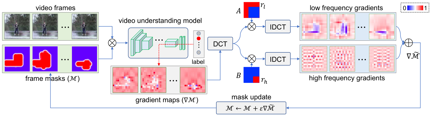
Therefore, we propose the Frequency-based Extremal Perturbation method (F-EP) which extends the EP method [Fong et al.(2019)Fong, Patrick, and Vedaldi] to the video domain. F-EP, illustrated in Fig. 1, aims to find the salient areas of the input by perturbing a mask, where the perturbations are the gradients of the output label with respect to the input. The masks, comprised of the aggregated perturbations, become the explanations for the video input. At each iteration of the optimization process, F-EP transforms the gradients into the frequency space using a common Fourier Transform: Discrete Cosine Transform (DCT). Then, F-EP modulates the frequency signals and transforms them back to the gradient space to update the masks.
This approach is inspired from works [Wang et al.(2020b)Wang, Wu, Yin, and Xing, Wallace(1992)] showing that neural networks not only learn the low-frequency components of an image, such as faces and shapes, but also the high-frequency components that appear like noise to humans. Therefore, the gradients of the salient high-frequency components will be high and make the gradient maps noisy. To overcome this problem, F-EP proposes to transform the gradients into the frequency domain and selects a combination of low and high frequency components of the gradients to achieve semantically meaningful explanations that are also faithful to the model. Meanwhile, because the explanations focus on the semantic features of each frame, such as a person performing an action, and the majority of frames contain these features, the explanations will naturally become spatiotemporally consistent.
Since no existing metrics address spatiotemporal consistency of explanations, we propose the Spatiotemporal Consistency (STC) metric to measure how well the explanations align with the ground truth bounding boxes. Because bounding boxes indicate the spatial position of the foreground object/scene, spatiotemporal consistent explanations will have high alignment with them. We experimentally show that F-EP achieves superior performance in terms of spatiotemporal consistency and faithfulness than the state-of-the-art methods. In summary, our contributions in this paper are as follows.
- •
We propose the F-EP method, which can simultaneously reduce the noise in the explanations and make them spatiotemporally consistent by modulating the gradients in the frequency space.
- •
We propose a new metric, Spatiotemporal Consistency (STC), to accurately assess the spatiotemporal consistency of an explanation in the video domain.
- •
In the ablation studies section, we show that F-EP using low frequency gradients is able to achieve state-of-the-art performance, while the addition of high-frequency gradients can improve its performance even further.
2 Related Work
Model explainability is increasingly popular in a diverse range of deep learning applications. In this section, we present only the methods for image and video recognition models.
Class Activation Map (CAM)-based. CAM-based methods, such as CAM [Zhou et al.(2016)Zhou, Khosla, Lapedriza, Oliva, and Torralba], Grad-CAM [Selvaraju et al.(2017)Selvaraju, Cogswell, Das, Vedantam, Parikh, and Batra], Grad-CAM++ [Chattopadhay et al.(2018)Chattopadhay, Sarkar, Howlader, and Balasubramanian], and Score-CAM [Wang et al.(2020a)Wang, Du, Yang, and Zhang], use weighted sums of either activation maps or gradients of the class label with respect the input to produce a heatmap. Although CAM-based methods are efficient [Desai and Ramaswamy(2020), Fu et al.(2020)Fu, Hu, Dong, Guo, Gao, and Li], usually requiring just a few forward and backward passes, the resulting heatmaps are coarse due to the upsampling process. The Saliency Tubes approach [Stergiou et al.(2019)Stergiou, Kapidis, Kalliatakis, Chrysoulas, Veltkamp, and Poppe] adapts Grad-CAM to the video domain.
Backprop-based. Backprop-based methods [Zeiler and Fergus(2014), Simonyan et al.(2014)Simonyan, Vedaldi, and Zisserman, Sundararajan et al.(2017)Sundararajan, Taly, and Yan, Smilkov et al.(2017)Smilkov, Thorat, Kim, Viégas, and Wattenberg, Montavon et al.(2017)Montavon, Lapuschkin, Binder, Samek, and Müller, Gu et al.(2019)Gu, Yang, and Tresp, Zhang et al.(2017)Zhang, Lin, Brandt, Shen, and Sclaroff, Adel Bargal et al.(2018)Adel Bargal, Zunino, Kim, Zhang, Murino, and Sclaroff] compute saliency scores for each input pixel by starting with the final layer and, one layer at a time, inferring the importance of the inputs to the outputs of the layer until the input is reached. For example, Layerwise Relevance Backpropagation (LRP)-based methods [Montavon et al.(2017)Montavon, Lapuschkin, Binder, Samek, and Müller, Gu et al.(2019)Gu, Yang, and Tresp] assign a relevance score for each neuron and backpropagate the relevance score of each neuron to the input layer. The explanations of backprop-based methods have been criticized for being similar to the results of an edge detector [Adebayo et al.(2018)Adebayo, Gilmer, Muelly, Goodfellow, Hardt, and Kim] and insensitive to randomization of the model’s parameters, which should intuitively alter the results [Sixt et al.(2019)Sixt, Granz, and Landgraf].
Perturbation-based. Perturbation-based explanation methods [Ribeiro et al.(2016)Ribeiro, Singh, and Guestrin, Petsiuk et al.(2018)Petsiuk, Das, and Saenko, Simonyan et al.(2014)Simonyan, Vedaldi, and Zisserman, Fong and Vedaldi(2017), Fong et al.(2019)Fong, Patrick, and Vedaldi, Wagner et al.(2019)Wagner, Kohler, Gindele, Hetzel, Wiedemer, and Behnke, Li et al.(2021)Li, Wang, Li, Huang, and Sato] add perturbations to the input features to quantify the importance of each pixel. For example, RISE [Petsiuk et al.(2018)Petsiuk, Das, and Saenko] measures the importance of pixels by randomly masking areas of input features and observing changes to the output. Meaningful Perturbation (MP) [Fong and Vedaldi(2017)] and Extremal Perturbation (EP) [Fong et al.(2019)Fong, Patrick, and Vedaldi] methods optimize masks as explanations to localize salient areas. STEP [Li et al.(2021)Li, Wang, Li, Huang, and Sato] extends EP to the video domain by adding spatiotemporal smoothness constraints, and it is the current state-of-the-art for explaining video understanding models. Although perturbation-based methods [Fong et al.(2019)Fong, Patrick, and Vedaldi, Li et al.(2021)Li, Wang, Li, Huang, and Sato] are able to produce more fine-grained explanations and are more sensitive to changes in the model’s weights compared to the CAM-based and backpropagation-based methods [Selvaraju et al.(2017)Selvaraju, Cogswell, Das, Vedantam, Parikh, and Batra, Chattopadhay et al.(2018)Chattopadhay, Sarkar, Howlader, and Balasubramanian, Simonyan et al.(2014)Simonyan, Vedaldi, and Zisserman, Sundararajan et al.(2017)Sundararajan, Taly, and Yan], their explanations are still noisy and not spatiotemporally consistent (see Fig. 10). Our proposed F-EP approach probes the frequency signals in the gradients in order to denoise the explanations and make them focus more tightly on the target object in every frame.
Fourier Transforms. Fourier transforms decompose a data point in the spatial or temporal domain into a combination of functions in the corresponding frequency domain. Discrete Cosine Transform (DCT) is a type of Fourier Transform using only real numbers. DCT was first proposed for efficient image compression, where only the content-defining features are preserved [Wallace(1992)]. DCT is used in machine learning for image compression with SVM [Karami et al.(2012)Karami, Beheshti, and Yazdi], image classification [Roy et al.(2017)Roy, Chakraborty, Sameer, and Naskar], and more. Recently, [Guo et al.(2020)Guo, Frank, and Weinberger, Sharma et al.(2019)Sharma, Ding, and Brubaker] explore the effectiveness of using DCT on crafting adversarial samples. Although F-EP is also using perturbation to produce explanations, the perturbations are added on the masks and not the inputs as in [Guo et al.(2020)Guo, Frank, and Weinberger, Sharma et al.(2019)Sharma, Ding, and Brubaker]. The optimization objectives are also different: adversarial attacks aim to generate samples to change the model’s prediction, while explanations aim to faithfully represent a model’s decision. Also, the adversarial samples are sparse, noisy and hard to interpret, while the explanations given by F-EP focus tightly on the target object/scene spatially and temporally.
3 Methodology
In this paper, F-EP is experimented on video classification models as in EP [Fong et al.(2019)Fong, Patrick, and Vedaldi]. A future research direction could be to evaluate F-EP on other types of video understanding models. Denote the video classification model by , the original input video clip as and the predicted label , where is among a set of classes, is the number of frames in a video clip, and are the height and width of the frame/mask, and is the number of channels. We first briefly introduce the baseline method, Extremal Perturbation (EP) [Fong et al.(2019)Fong, Patrick, and Vedaldi], and then explain our proposed Frequency-based Extremal Perturbation (F-EP) method, which is shown in Fig. 1.
3.1 Extremal Perturbation
Extremal Perturbation (EP) was proposed to explain image understanding models and aims to localize the salient areas in the input for a model’s decision through perturbations on the masks. Let the masks be , the optimization objective of EP is:
| (1) |
The left term in Eq. (1) maximizes the classification confidence of the model to the perturbed input . The operator is the perturbation operator which applies local Gaussian blurring to each pixel in . The second term in Eq. (1) is , which regularizes the area of the mask with respect to the area constant . is the regularizer constant. is a binarized vector with ones and zeros, and is sorted vector of the masks . Thus, computes the loss of the area of masks with respect to the area constraint . To solve the optimization problem (1), we can derive the gradients of the output class label with respect to the masks where is the learning rate of the optimization (details in [Fong et al.(2019)Fong, Patrick, and Vedaldi]):
| (2) |
The optimal solution thus can be approximated by an iterative gradient ascent process. In each iteration, the masks are updated as follows:
| (3) |
3.2 Frequency-based Extremal Perturbation
[EP [Fong et al.(2019)Fong, Patrick, and Vedaldi] Gradient Maps]


 \subfigure[F-EP Gradient Maps]


[Original, CricketBowling, 0.59]


 \subfigure[EP [Fong et al.(2019)Fong, Patrick, and Vedaldi], CricketBowling, 1.0]


 \subfigure[F-EP, CricketBowling, 0.85]


Motivation. A model explanation is expected to be interpretable by people and faithfully represent a model’s inference process [Gunning and Aha(2019)]. This becomes a challenge when the neural network not only uses low-frequency features for learning larger shapes and objects like faces, but also high-frequency features that look like noise [Wang et al.(2020b)Wang, Wu, Yin, and Xing]. Because EP aims to achieve higher model confidence regardless of the the frequencies chosen, thus the high frequency features are included if they are more salient than the low frequency features which make explanations noisy and not spatiotemporally consistent.
Because the gradients encode the importance of each pixel (Eq. (2)), important high-frequency features would have high gradients in , making noisy. A noisy leads to noisy explanations , since the latter is iteratively updated with the former, as shown in Eq. (3). We propose to transform the gradients into the frequency domain using the Discrete Cosine Transform (DCT), such that the signals related to the content-defining features, which reside in the lower end of the spectrum of the frequencies [Wallace(1992)], are preserved. High-frequency signals are not only associated with noise, but also the fine-grained details such as textures/edges. Thus, the low frequency signals allow the explanations to focus on the target object/person and become spatiotemporal consistent, while the high frequency features make the explanations more faithful to the model and fine-grained, see Fig. 3. The Fig. 2 shows that the frequency modulated gradient maps focus more on the foreground object and become spatiotemporal consistent when consecutive frames contain the target object. In the following section, we propose our method Frequency-based Extremal Perturbation (F-EP) and theoretically demonstrate that modulating gradients is equivalent to modulating the masks.
Gradient Frequency Modulation. F-EP is presented in Fig. 1. At each iteration of the optimization, F-EP transforms the gradient maps into the frequency domain using DCT. DCT is chosen over Discrete Fourier Transform (DFT) because the basis functions used in DFT are complex-valued, while only contains real numbers, meaning that DFT would compute useless transformations [Blinn(1993)]. Because is three dimensional, the DCT is also three dimensional. Denote the DCT as and the frequency map of the gradient as , the -th spatio-temporal entry of , , and is computed by the three-dimensional DCT:
| (4) |
where is a constant and is the cosine basis function, if , otherwise . is the vector form of the element-wise product between the vector and along -axis, i.e., . The definitions of , , and are similar to , , and . Thus, Eq. (4) shows that the DCT operation is an intrinsically linear system, and according to the gradient ascent rule in Eq. (3), we have the following equality:
| (5) |
This equation shows that applying frequency modulation on the gradient map is equivalent to frequency modulation on the optimal mask . We provide a more detailed derivation in the supplementary material. Therefore, it is straightforward to linearly modulate the gradient frequency map . To this end, we perform the frequency modulation on as follows:
| (6) |
where is the inverse DCT (IDCT) function and is the element-wise product. Note both are linear systems. The low frequency mask is defined as if , otherwise zero, and the high frequency mask is defined as if , otherwise one. See the and matrices in Fig. 1. and denote the ratios of low- and high-frequency components to be preserved, respectively. Note that and .
Eq. (6) first selects a ratio of low-end frequencies and a ratio of high-end frequencies from , then performs IDCT on the selected high and low frequencies separately. By summing up the gradients maps modulated at different frequencies, we ensure that the gradient information contains both the low-end and high-end features.
Finally, instead of using the raw gradient in equation (3), we propose to use the frequency-modulated gradient such that:
| (7) |
Since DCT and IDCT are computationally efficient, our proposed modulation does not incur too much computational cost.
4 Experiment
4.1 Experimental Settings
Evaluation Metrics. Evaluation has always been one of the most challenging parts of studying model explainability. Due to the lack of ground truth explanations, existing methods can only be evaluated in a post hoc manner. We follow prior work in using two standard metrics that also apply to static images. First, Drop in Confidence (DC) measures the decrease in model’s confidence on the explanations compared to the original input [Chattopadhay et al.(2018)Chattopadhay, Sarkar, Howlader, and Balasubramanian] (smaller DC is better). It is represented as where and as in Eq. (1). Second, Accuracy (Acc.) measures the model’s classification accuracy on the explanations .
In addition, since no existing evaluation metric is suitable to assess the spatiotemporal consistency of an explanation, we propose a new metric called Spatiotemporal Consistency (STC). STC calculates the overlap between the explanations and the ground truth bounding boxes. Mathematically, we define , where are the ground truth bounding boxes where for all pixels inside the bounding boxes, and 0 otherwise. denotes the threshold of masks during evaluation because are continuous values within range . Because the bounding boxes focus tightly on the foreground object/person in each frame, a more spatiotemporally consistent explanation will have higher overlap with them.
Experimental Details We evaluate F-EP against CAM-based methods: Grad-CAM [Selvaraju et al.(2017)Selvaraju, Cogswell, Das, Vedantam, Parikh, and Batra] and Grad-CAM++ [Chattopadhay et al.(2018)Chattopadhay, Sarkar, Howlader, and Balasubramanian], and backpropagation-based methods: Gradients [Simonyan et al.(2014)Simonyan, Vedaldi, and Zisserman], Integrated Grad [Sundararajan et al.(2017)Sundararajan, Taly, and Yan] and Smooth Grad [Smilkov et al.(2017)Smilkov, Thorat, Kim, Viégas, and Wattenberg]. We extend the original implementation of these methods11 1 https://github.com/jacobgil/pytorch-grad-cam to the video domain. EP [Fong et al.(2019)Fong, Patrick, and Vedaldi] was extended to the video domain in STEP [Li et al.(2021)Li, Wang, Li, Huang, and Sato] 22 2 https://github.com/shinkyo0513/Video-Visual-Explanations. The target models to be explained are R(2+1)D [Tran et al.(2018)Tran, Wang, Torresani, Ray, LeCun, and Paluri] and TSM [Lin et al.(2019)Lin, Gan, and Han].33 3 https://github.com/open-mmlab/mmaction2 For video datasets, we use UCF101-24 [Soomro et al.(2012)Soomro, Zamir, Shah, Soomro, Zamir, and Shah] and Epic-Kitchens-Object [Damen et al.(2018)Damen, Doughty, Farinella, Fidler, Furnari, Kazakos, Moltisanti, Munro, Perrett, Price, and Wray]. UCF101-24 is a video understanding dataset of 24 actions with annotated bounding boxes and Epic-Kitchens-Object records cooking activities from a first-person point of view. The hyperparameters used are the same as in STEP [Li et al.(2021)Li, Wang, Li, Huang, and Sato], except the step size is 13 and sigma is 23. The parameters and are selected based on the best performance on the validation set.
4.2 Quantitative Results
Figure 6: DAUC of all the compared methods, which plots the model’s confidence drop with respect to the percentage of pixels deleted. Note that the most salient pixels are deleted first. Lower Area Under the Curve (AUC) is better. F-EP has the lowest AUC compared to other methods, which indicates that the features contained in the explanations are more salient.
| Method | R(2+1)D | TSM | ||||
|---|---|---|---|---|---|---|
| DC () | Acc. () | STC () | DC () | Acc. () | STC () | |
| Gradients [Simonyan et al.(2014)Simonyan, Vedaldi, and Zisserman] | 89.4 | 6.0 | 0.4 | 90.8 | 2.1 | 0.6 |
| Integrated Grad [Sundararajan et al.(2017)Sundararajan, Taly, and Yan] | 89.5 | 6.9 | 0.5 | 89.5 | 4.0 | 1.2 |
| Smooth Grad [Smilkov et al.(2017)Smilkov, Thorat, Kim, Viégas, and Wattenberg] | 90.7 | 1.0 | 1.8 | 90.7 | 2.7 | 1.2 |
| Grad-CAM [Selvaraju et al.(2017)Selvaraju, Cogswell, Das, Vedantam, Parikh, and Batra] | 42.7 | 58.1 | 28.9 | 88.6 | 11.2 | 0.1 |
| Grad-CAM++ [Chattopadhay et al.(2018)Chattopadhay, Sarkar, Howlader, and Balasubramanian] | 42.3 | 58.3 | 35.1 | 24.1 | 74.8 | 17.4 |
| EP [Fong et al.(2019)Fong, Patrick, and Vedaldi] | 37.9 | 61.7 | 63.8 | 40.0 | 63.0 | 70.6 |
| STEP [Li et al.(2021)Li, Wang, Li, Huang, and Sato] | 34.2 | 67.1 | 63.8 | 39.9 | 65.2 | 73.9 |
| F-EP (ours) | 32.9 | 73.4 | 67.0 | 33.3 | 71.0 | 74.6 |
UCF101-24 Results. Table 1 presents F-EP against SOTA methods on the UCF101-24 [Soomro et al.(2012)Soomro, Zamir, Shah, Soomro, Zamir, and Shah] dataset based on two target models, R(2+1)D [Tran et al.(2018)Tran, Wang, Torresani, Ray, LeCun, and Paluri] and TSM [Lin et al.(2019)Lin, Gan, and Han]. The outperformance of F-EP (, ) on the R(2+1)D model shows that it is able to produce more faithful and spatiotemporal consistent explanations than all the other methods, including the baselines EP [Fong et al.(2019)Fong, Patrick, and Vedaldi] and STEP [Li et al.(2021)Li, Wang, Li, Huang, and Sato]. On TSM, F-EP (, ) achieves best on the STC metric, and second best on the DC and Acc. metrics. The first reason is that the UCF101-24 dataset has high scene representation bias [Choi et al.(2019)Choi, Gao, Messou, and Huang], and the model needs not to look at the actual activity to give a correct prediction. Because the explanations given by F-EP focus more on the person performing the activity, which are at the lower end of the frequency domain, the model will have lower confidence on these explanations. Second, R(2+1)D uses 3D convolution filters to extract spatiotemporal features, while TSM uses 2D convolution filters that capture less temporal information. Thus, a more spatiotemporally consistent explanation will have higher model confidence in R(2+1)D than TSM.
Fig. 6 illustrates the Deletion metric [Petsiuk et al.(2018)Petsiuk, Das, and Saenko], which measures the drop in model’s confidence when the most important pixels are removed. The importance of pixels are given by the saliency maps. A lower Area Under the Curve (AUC) implies the explanation method is better and the saliency features contained are more faithful to the model. We see that F-EP has the lowest AUC compared to other explanation methods.
| Method | DC () | Acc. () | STC () |
|---|---|---|---|
| Gradients [Simonyan et al.(2014)Simonyan, Vedaldi, and Zisserman] | 48.1 | 16.0 | 0.4 |
| Integrated Grad [Sundararajan et al.(2017)Sundararajan, Taly, and Yan] | 49.0 | 5.5 | 0.4 |
| Smooth Grad [Smilkov et al.(2017)Smilkov, Thorat, Kim, Viégas, and Wattenberg] | 49.3 | 6.1 | 0.8 |
| Grad-CAM [Selvaraju et al.(2017)Selvaraju, Cogswell, Das, Vedantam, Parikh, and Batra] | 28.3 | 48.0 | 27.2 |
| Grad-CAM++ [Chattopadhay et al.(2018)Chattopadhay, Sarkar, Howlader, and Balasubramanian] | 54.8 | 42.1 | 30.6 |
| EP [Fong et al.(2019)Fong, Patrick, and Vedaldi] | 34.2 | 43.4 | 58.0 |
| STEP [Li et al.(2021)Li, Wang, Li, Huang, and Sato] | 32.6 | 43.8 | 61.0 |
| F-EP (ours) | 32.4 | 44.4 | 67.8 |
Epic-Kitchens-Objects Results. Table 2 reports the results of R(2+1)D on the Epic-Kitchens-Object [Damen et al.(2018)Damen, Doughty, Farinella, Fidler, Furnari, Kazakos, Moltisanti, Munro, Perrett, Price, and Wray] dataset. F-EP (, ) performs slightly less well on DC and Acc than Grad-CAM, but much better in STC (Qualitative results are shown in the supplemental material). The explanations given by F-EP have lower model confidence because videos in the Epic-Kitchens-Object dataset do not contain the target object in every frame but F-EP produces explanation for each frame. Therefore, non-target objects are included in the explanations which have lower model confidence. A future research direction is to have the optimization algorithm attend only to salient frames for the output decision.
Tables 1 and 2 show that backpropagation-based methods, Gradients [Simonyan et al.(2014)Simonyan, Vedaldi, and Zisserman], Integrated Grad [Sundararajan et al.(2017)Sundararajan, Taly, and Yan] and SmoothGrad [Smilkov et al.(2017)Smilkov, Thorat, Kim, Viégas, and Wattenberg], perform poorly compared to CAM- and perturbation-based methods. For example, Fig. 10’s second row (more results in the supplement) shows that Integrated Grad’s explanations consist of sparse pixels that align poorly with the ground truth. These explanations are often perceived by the model as adversarial samples and have lower model confidence or even incorrect predicted labels [Ian Goodfellow(2014)]. SmoothGrad and Gradients produce similar explanations and hence face the same problems.
Figure 9: Performance comparison of different and . The vertical series of circles show the performance of with increasing . Note that . The horizontal series of circles show when with increasing . EP [Fong et al.(2019)Fong, Patrick, and Vedaldi] is the lower right circle.
4.3 Ablation Studies
| Input |  |
 |
 |
 |
 |
 |
 |
FG, [0.63] |
| Grad-CAM [Selvaraju et al.(2017)Selvaraju, Cogswell, Das, Vedantam, Parikh, and Batra] |  |
 |
 |
 |
 |
 |
 |
BB, [0.19] |
| Integrated [Sundararajan et al.(2017)Sundararajan, Taly, and Yan] |  |
 |
 |
 |
 |
 |
|
WB, [0.37] |
| EP [Fong et al.(2019)Fong, Patrick, and Vedaldi] |  |
 |
 |
 |
 |
 |
 |
BB, [0.99] |
| STEP [Li et al.(2021)Li, Wang, Li, Huang, and Sato] |  |
 |
 |
 |
 |
|
 |
BB, [0.87] |
| F-EP (ours) |  |
 |
 |
 |
 |
 |
 |
FG, [0.76] |
Without High Frequency. In Fig. 9, when and as increases, the STC performance increases because the higher frequency signals encode the details such as edges/textures to increase faithfulness of explanations. There is a sharp drop in performance after , because as contains more and more higher frequency signals, it is overwhelmed with the excess amount of details. The explanations also become noisier and less spatiotemporal consistent, because higher frequency features are preferred over the low frequency features if they could increase more model confidence.
Combination of High and Low Frequencies. We conduct experiments with varying and deterministic . When , as increases, STC increases because the amount of frequency signals on the lower end frequency spectrum is not enough and higher frequency signals add valuable information to the explanations. However, when , STC performance increases less quickly than . This could mean that is a threshold at which the utility of high frequency signals decreases. Finally, when , STC actually decreases when increases. Also, F-EP is able to outperform the baseline method EP at multiple combination of frequencies which confirms our hypothesis that not all frequency signals are salient. One future work direction is to search the appropriate ratios and for each sample because samples vary across dataset and actions.
4.4 Qualitative Results
In Fig. 10, we see that the explanations produced by F-EP are much easier to interpret than those of the prior works. Integrated Grad explanations are noisy, sparse and difficult to interpret, because it directly uses gradients, which contain a substantial amount of noise. Grad-CAM produces explanations that fail to capture the activity dynamics. EP and STEP has difficulty in correctly capturing the person’s movement in the consecutive frames. In comparison, F-EP is able to produce explanations that focus on the person performing the activity on each frame (more qualitative results are in the supplement).
5 Conclusion
In this paper, we propose an explanation method for video understanding models called Frequency-based Extremal Perturbation (F-EP) which aims to produce spatiotemporal consistent explanations that are faithful to the model and interpretable by humans. F-EP transforms the gradients to the frequency domain and modulates the frequency signals in order to preserve those gradient components that help to explain a model’s decision. We experiment F-EP on various datasets and models and show that F-EP is able to outperform existing state-of-the-art works.
Acknowledgments. This work is supported in part by the John S. and James L. Knight Foundation, the Miami Foundation through the Ethics and Governance of the Artificial Intelligence Initiative, the National Science Foundation under award No. 2040209, and the Army Research Office under grant number W911NF-21-1-0236.
References
- [Adebayo et al.(2018)Adebayo, Gilmer, Muelly, Goodfellow, Hardt, and Kim] Julius Adebayo, Justin Gilmer, Michael Muelly, Ian Goodfellow, Moritz Hardt, and Been Kim. Sanity checks for saliency maps. In NeurIPS, 2018.
- [Adel Bargal et al.(2018)Adel Bargal, Zunino, Kim, Zhang, Murino, and Sclaroff] Sarah Adel Bargal, Andrea Zunino, Donghyun Kim, Jianming Zhang, Vittorio Murino, and Stan Sclaroff. Excitation backprop for rnns. In CVPR, 2018.
- [Blinn(1993)] J.F. Blinn. What’s that deal with the dct? IEEE Computer Graphics and Applications, 13, 1993.
- [Chattopadhay et al.(2018)Chattopadhay, Sarkar, Howlader, and Balasubramanian] Aditya Chattopadhay, Anirban Sarkar, Prantik Howlader, and Vineeth N Balasubramanian. Grad-cam++: Generalized gradient-based visual explanations for deep convolutional networks. In WACV, 2018.
- [Cho et al.(2014)Cho, van Merriënboer, Bahdanau, and Bengio] Kyunghyun Cho, Bart van Merriënboer, Dzmitry Bahdanau, and Yoshua Bengio. On the properties of neural machine translation: Encoder–decoder approaches. In Proceedings of SSST-8, Eighth Workshop on Syntax, Semantics and Structure in Statistical Translation, pages 103–111, Doha, Qatar, October 2014. Association for Computational Linguistics. 10.3115/v1/W14-4012. URL https://www.aclweb.org/anthology/W14-4012.
- [Choi et al.(2019)Choi, Gao, Messou, and Huang] Jinwoo Choi, Chen Gao, C. E. Joseph Messou, and Jia-Bin Huang. Why can’t i dance in the mall? learning to mitigate scene bias in action recognition. In NeurIPS, 2019.
- [Damen et al.(2018)Damen, Doughty, Farinella, Fidler, Furnari, Kazakos, Moltisanti, Munro, Perrett, Price, and Wray] Dima Damen, Hazel Doughty, Giovanni Maria Farinella, Sanja Fidler, Antonino Furnari, Evangelos Kazakos, Davide Moltisanti, Jonathan Munro, Toby Perrett, Will Price, and Michael Wray. Scaling egocentric vision: The epic-kitchens dataset. In ECCV, 2018.
- [Deng et al.(2009)Deng, Dong, Socher, Li, Kai Li, and Li Fei-Fei] J. Deng, W. Dong, R. Socher, L. Li, Kai Li, and Li Fei-Fei. Imagenet: A large-scale hierarchical image database. In CVPR, 2009.
- [Desai and Ramaswamy(2020)] Saurabh Desai and Harish G. Ramaswamy. Ablation-cam: Visual explanations for deep convolutional network via gradient-free localization. In WACV, 2020.
- [Dzindolet et al.(2003)Dzindolet, Peterson, Pomranky, Pierce, and Beck] Mary T. Dzindolet, Scott A. Peterson, Regina A. Pomranky, Linda G. Pierce, and Hall P. Beck. The role of trust in automation reliance. Int. J. Hum.-Comput. Stud., 58, 2003.
- [Fong et al.(2019)Fong, Patrick, and Vedaldi] Ruth Fong, Mandela Patrick, and Andrea Vedaldi. Understanding deep networks via extremal perturbations and smooth masks. In ICCV, 2019.
- [Fong and Vedaldi(2017)] Ruth C. Fong and Andrea Vedaldi. Interpretable explanations of black boxes by meaningful perturbation. In ICCV, 2017.
- [Fu et al.(2020)Fu, Hu, Dong, Guo, Gao, and Li] Ruigang Fu, Qingyong Hu, Xiaohu Dong, Yulan Guo, Yinghui Gao, and Biao Li. Axiom-based grad-cam: Towards accurate visualization and explanation of cnns. In BMVC, 2020.
- [Gu et al.(2019)Gu, Yang, and Tresp] Jindong Gu, Yinchong Yang, and Volker Tresp. Understanding individual decisions of cnns via contrastive backpropagation. In ACCV, 2019.
- [Gunning and Aha(2019)] David Gunning and David Aha. Darpa’s explainable artificial intelligence (xai) program. AI Magazine, 40, 2019. URL https://ojs.aaai.org/index.php/aimagazine/article/view/2850.
- [Guo et al.(2020)Guo, Frank, and Weinberger] Chuan Guo, Jared S. Frank, and Kilian Q. Weinberger. Low frequency adversarial perturbation. In Proceedings of The Uncertainty in Artificial Intelligence Conference, 2020.
- [Ian Goodfellow(2014)] Christian Szegedy Ian Goodfellow, Jon Shlens. Explaining and harnessing adversarial examples. In ICLR, 2014.
- [Karami et al.(2012)Karami, Beheshti, and Yazdi] Azam Karami, Soosan Beheshti, and Mehran Yazdi. Hyperspectral image compression using 3d discrete cosine transform and support vector machine learning. In ISSPA, 2012.
- [Li et al.(2021)Li, Wang, Li, Huang, and Sato] Zhenqiang Li, Weimin Wang, Zuoyue Li, Yifei Huang, and Yoichi Sato. Towards visually explaining video understanding networks with perturbation. In WACV, 2021.
- [Lin et al.(2019)Lin, Gan, and Han] Ji Lin, Chuang Gan, and Song Han. Tsm: Temporal shift module for efficient video understanding. In ICCV, 2019.
- [Lipton(2018)] Zachary C. Lipton. The mythos of model interpretability: In machine learning, the concept of interpretability is both important and slippery. Queue, 16, 2018.
- [Lombrozo(2006)] Tania Lombrozo. The structure and function of explanations. Trends in cognitive sciences, 10, 2006.
- [Montavon et al.(2017)Montavon, Lapuschkin, Binder, Samek, and Müller] Grégoire Montavon, Sebastian Lapuschkin, Alexander Binder, Wojciech Samek, and Klaus-Robert Müller. Explaining nonlinear classification decisions with deep taylor decomposition. Pattern Recognition, 65, 2017.
- [Petsiuk et al.(2018)Petsiuk, Das, and Saenko] Vitali Petsiuk, Abir Das, and Kate Saenko. Rise: Randomized input sampling for explanation of black-box models. In British Machine Vision Conference (BMVC), 2018.
- [Ribeiro et al.(2016)Ribeiro, Singh, and Guestrin] Marco Tulio Ribeiro, Sameer Singh, and Carlos Guestrin. ”why should i trust you?”: Explaining the predictions of any classifier. In Proceedings of the 22nd ACM SIGKDD International Conference on Knowledge Discovery and Data Mining, 2016.
- [Richens et al.(2020)Richens, Lee, and Johri] Jonathan G. Richens, Ciarán M. Lee, and Saurabh Johri. Improving the accuracy of medical diagnosis with causal machine learning. Nature Communications, 11, 2020.
- [Roy et al.(2017)Roy, Chakraborty, Sameer, and Naskar] Aniket Roy, Rajat Subhra Chakraborty, Udaya Sameer, and Ruchira Naskar. Camera source identification using discrete cosine transform residue features and ensemble classifier. In CVPRW, 2017.
- [Selvaraju et al.(2017)Selvaraju, Cogswell, Das, Vedantam, Parikh, and Batra] Ramprasaath R Selvaraju, Michael Cogswell, Abhishek Das, Ramakrishna Vedantam, Devi Parikh, and Dhruv Batra. Grad-cam: Visual explanations from deep networks via gradient-based localization. In ICCV, 2017.
- [Sharma et al.(2019)Sharma, Ding, and Brubaker] Yash Sharma, Gavin Weiguang Ding, and Marcus A. Brubaker. On the effectiveness of low frequency perturbations. In IJCAI, 2019.
- [Shen et al.(2019)Shen, Margolies, Rothstein, Fluder, McBride, and Sieh] Li Shen, Laurie R. Margolies, Joseph H. Rothstein, Eugene Fluder, Russell McBride, and Weiva Sieh. Deep learning to improve breast cancer detection on screening mammography. Scientific Reports, 9, 2019.
- [Simonyan et al.(2014)Simonyan, Vedaldi, and Zisserman] Karen Simonyan, Andrea Vedaldi, and Andrew Zisserman. Deep inside convolutional networks: Visualising image classification models and saliency maps. In ICLR Workshop, 2014.
- [Sixt et al.(2019)Sixt, Granz, and Landgraf] Leon Sixt, Maximilian Granz, and Tim Landgraf. When explanations lie: Why modified BP attribution fails. In ICML, 2019.
- [Smilkov et al.(2017)Smilkov, Thorat, Kim, Viégas, and Wattenberg] Daniel Smilkov, Nikhil Thorat, Been Kim, Fernanda Viégas, and Martin Wattenberg. SmoothGrad: removing noise by adding noise. In ICML Workshop, 2017.
- [Soomro et al.(2012)Soomro, Zamir, Shah, Soomro, Zamir, and Shah] Khurram Soomro, Amir Roshan Zamir, Mubarak Shah, Khurram Soomro, Amir Roshan Zamir, and Mubarak Shah. Ucf101: A dataset of 101 human actions classes from videos in the wild. CoRR, abs/1212.0402, 2012.
- [Springenberg et al.(2015)Springenberg, Dosovitskiy, Brox, and Riedmiller] J.T. Springenberg, A. Dosovitskiy, T. Brox, and M. Riedmiller. Striving for simplicity: The all convolutional net. In ICLR Workshop, 2015.
- [Stergiou et al.(2019)Stergiou, Kapidis, Kalliatakis, Chrysoulas, Veltkamp, and Poppe] Alexandros Stergiou, Georgios Kapidis, Grigorios Kalliatakis, Christos Chrysoulas, Remco Veltkamp, and Ronald Poppe. Saliency tubes: Visual explanations for spatio-temporal convolutions. In ICIP, 2019.
- [Sundararajan et al.(2017)Sundararajan, Taly, and Yan] Mukund Sundararajan, Ankur Taly, and Qiqi Yan. Axiomatic attribution for deep networks. In ICML, 2017.
- [Tania(2011)] Lombrozo Tania. The instrumental value of explanations. Philosophy Compass, 6, 2011.
- [Tran et al.(2014)Tran, Bourdev, Fergus, Torresani, and Paluri] Du Tran, Lubomir Bourdev, Rob Fergus, Lorenzo Torresani, and Manohar Paluri. Learning spatiotemporal features with 3d convolutional networks. In ICCV, 2014.
- [Tran et al.(2018)Tran, Wang, Torresani, Ray, LeCun, and Paluri] Du Tran, Heng Wang, Lorenzo Torresani, Jamie Ray, Yann LeCun, and Manohar Paluri. A closer look at spatiotemporal convolutions for action recognition. In CVPR, 2018.
- [Verhelst et al.(2020)Verhelst, Stannat, and Mecacci] H. M. Verhelst, A. W. Stannat, and G. Mecacci. Machine learning against terrorism: How big data collection and analysis influences the privacy-security dilemma. Science and Engineering Ethics, 26, 2020.
- [Wagner et al.(2019)Wagner, Kohler, Gindele, Hetzel, Wiedemer, and Behnke] Jorg Wagner, Jan Mathias Kohler, Tobias Gindele, Leon Hetzel, Jakob Thaddaus Wiedemer, and Sven Behnke. Interpretable and fine-grained visual explanations for convolutional neural networks. In CVPR, 2019.
- [Wallace(1992)] G.K. Wallace. The jpeg still picture compression standard. IEEE Transactions on Consumer Electronics, 38, 1992.
- [Wang et al.(2020a)Wang, Du, Yang, and Zhang] Haofan Wang, Mengnan Du, Fan Yang, and Zijian Zhang. Score-cam: Improved visual explanations via score-weighted class activation mapping. In CVPRW, 2020a.
- [Wang et al.(2020b)Wang, Wu, Yin, and Xing] Haohan Wang, Xindi Wu, Pengcheng Yin, and Eric P. Xing. High frequency component helps explain the generalization of convolutional neural networks. In CVPR, 2020b.
- [Zeiler and Fergus(2014)] Matthew D. Zeiler and Rob Fergus. Visualizing and understanding convolutional networks. In ECCV, 2014.
- [Zhang et al.(2017)Zhang, Lin, Brandt, Shen, and Sclaroff] Jianming Zhang, Zhe Lin, Jonathan Brandt, Xiaohui Shen, and Stan Sclaroff. Top-down neural attention by excitation backprop. IJCV, 126, 2017.
- [Zhou et al.(2016)Zhou, Khosla, Lapedriza, Oliva, and Torralba] Bolei Zhou, Aditya Khosla, Agata Lapedriza, Aude Oliva, and Antonio Torralba. Learning deep features for discriminative localization. In CVPR, 2016.