DESY 21-134
Kination cosmology from scalar fields
and gravitational-wave signatures
Yann Gouttenoirea, Géraldine Servantb,c, Peera Simakachornb,c
a School of Physics and Astronomy, Tel-Aviv University, Tel-Aviv 69978, Israel
b Deutsches Elektronen-Synchrotron DESY, Notkestraße 85, 22607, Hamburg, Germany
c II. Institute of Theoretical Physics, Universität Hamburg, 22761, Hamburg, Germany
Abstract
Kination denotes an era in the cosmological history corresponding to an equation of state such that the total energy density of the universe redshifts as the sixth inverse power of the scale factor. This arises if the universe is dominated by the kinetic energy of a scalar field. It has often been motivated in the literature as an era following inflation, taking place before the radiation era. In this paper, we review instead the possibility that kination is disconnected from primordial inflation and occurs much later, inside the Standard Model radiation era. We study the implications on all main sources of primordial gravitational waves. We show how this leads to very distinctive peaked spectra in the stochastic background of long-lasting cosmological sources of gravitational waves, namely the irreducible gravitational waves from inflation, and gravitational waves from cosmic strings, both local and global, with promising observational prospects. We present model-independent signatures and detectability predictions at SKA, LIGO, LISA, ET, CE, BBO, as a function of the energy scale and duration of the kination era. We then argue that such intermediate kination era is in fact symptomatic in a large class of axion models. We analyse in details the scalar field dynamics, the working conditions and constraints in the underlying models. We present the gravitational-wave predictions as a function of particle physics parameters. We derive the general relation between the gravitational-wave signal and the axion dark matter abundance as well as the baryon asymmetry. We investigate the predictions for the special case of the QCD axion. The key message is that gravitational-waves of primordial origin represent an alternative experimental probe of axion models.
1 Introduction
The measurement of the abundances of the light elements as predicted by the theory of Big-Bang Nucleosynthesis (BBN) constrains the universe to be dominated by radiation when the temperature was MeV. The smoothness and flatness of the universe, and the temperature anisotropies in the Cosmic Microwave Background (CMB), support the idea that much earlier than BBN, the universe was inflating exponentially, dominated by the energy density of a slowly-rolling scalar field. The non-detection of the fundamental B-mode polarization patterns in the CMB suggest that the maximal Hubble rate during inflation is GeV, which corresponds to a maximal energy scale of GeV [1, 2, 3].
The equation of state (EOS) of the universe between the end of inflation and the onset of BBN, encoded by the parameter , where and are the local pressure and energy densities, is currently unconstrained [4]. While the standard paradigm assumes that the energy density of the post-inflationary universe is radiation-dominated, , alternative cosmological histories are not unlikely. For instance, the dynamics of the inflaton at the end of inflation can trigger a stiff EOS, such that the total energy density of the universe redshifts faster than radiation. In this scenario, the universe can be dominated by the kinetic energy of a fast-rolling scalar field, with [5, 6, 7, 8].
The possibility that the universe has had a stiff EOS, , is particularly relevant for the observation of a Stochastic Background of Gravitational Waves (SGWB) of primordial origin. The main sources of gravitational waves (GW) in the early universe are inflation, reheating/preheating, first-order phase transitions, and cosmic strings [9]. The observation of such GW in future interferometers or at pulsar-timing arrays would not only offer a unique probe of the high-energy particle physics phenomena responsible for their production but also of the cosmological history, as the GW spectra encode information about the EOS of the universe between GW production at very early times and GW detection today.
The interesting aspect of an era with a stiff EOS is that it leads to an amplification of the GW energy density produced by long-lasting sources compared to the predicted value in standard cosmology. This can be understood as follows. A given GW frequency in the primordial GW spectrum measured today corresponds to a GW emitted at time with frequency of order when the total energy density of the universe . Reading the frequency spectrum from low to high frequencies is like going back to earlier emission times. The emitted energy density in GW is proportional to , and therefore to . For a given GW frequency today, the corresponding total energy density of the universe is necessarily higher in the scenario with a kination era than in the standard cosmology, see Fig. 1. If a stiff era occurred, the GW energy density today is larger than the value obtained assuming standard cosmology. If a stiff era lasts too long, this leads to a substantial amplification of the primordial GW signal, violating the bounds on the number of massless degrees of freedom from BBN. There is a large literature on the impact of a stiff era on the nearly-scale invariant primordial GW spectrum generated during inflation in the case where kination happens right after inflation [10, 11, 12, 13, 14, 15, 16, 17, 18, 19, 20, 21, 22, 23, 24, 25, 26, 27, 28, 29, 23, 30]. The effect of a kination era following inflation on the SGWB generated by cosmic strings was also discussed in [31, 32, 33, 34, 35, 36, 37].
On the other hand, so far (up to the suggestions in [38, 39] and the coincident studies [40, 41]), there has been no investigation of the scenario where kination is disconnected from inflation and happens much later after reheating, inside the radiation era. In this situation, BBN- bounds are easily evaded, while the observational prospects at future gravitational-wave observatories are excellent. This is the main topic of this article. Such scenario can be realised only if the kination era is preceeded by a matter era. The main task of this paper is to motivate, from particle physics, such a scenario, to derive the GW signatures and the prospects for their detectability. We identify main classes of models where this happens naturally. They are linked to axion models where the axion acquires a large kinetic energy before its low-energy potential develops, therefore leading to a spinning stage along the circular orbit of the axion potential. The interplayed dynamics between the radial mode and the angular mode of a complex scalar field generates the desired sequence of events. A letter version of this work was presented in [40]. We provide many details and a thorough discussion in this paper, in particular on the damping of radial motion.
The plan of this paper is the following. We start with the phenomenology and the observational implications of a kination era. We then present the particle physics implementation. In Sec. 2, we review the status of kination in a broad sense, we sketch the three possible cosmological scenarios that can lead to a kination era. We first discuss the universal experimental prospects for probing a kination era following inflation: We derive in Fig. 2 the values of the inflation scale and of the reheating temperature that are already constrained by BBN and by the scalar fluctuation, concluding that LIGO, LISA, ET and BBO do not have sensitivity to probe the allowed region of parameter space and only ultra-high-frequency experiments could do so. We then turn to our main topic: a kination era inside the radiation era. Gravitational-wave signatures are first studied in a model-independent way in Sec. 3. We predict the effect of kination on the irreducible GW spectrum from inflation as well as on the GW from (both local and global) cosmic strings. We present the constraints on the duration and energy scale of kination. Prospects for detection at future experiments are derived in detail. Having motivated an intermediate kination era with axion models, we determine the relation between the relic abundance of the axion and the GW energy density today in Sec. 4. We also comment on the relation between the GW energy density today and the baryonic energy density predicted through the axiogenesis mechanism in Sec. 5. We then discuss the particle physics realisations in Sec. 6 , 7, 8, 9 and 10. The damping of the radial mode energy density is a crucial aspect in this story and we discuss this extensively in Sec. 8 and 9 and 10. Thermal effects are investigated in details in Sec. 9 and 10. The conditions that lead to kination are analysed in terms of model parameters for both classes of models. Precise predictions for the GW signal and the prospects for detection for each class of models are given. We conclude in Sec. 11.
A number of technical details are presented in the appendices. App. A reviews the occurrence of a kination era following inflation before reheating. App. B shows the constraints and observability prospects of a generic stiff era with EOS . App. C discusses different limitations on the duration of a kination era. App. D explains in details the origin of the complex scalar potential in the UV completion and the role of each term in the dynamics. In App. E, we discuss the usual issues of adiabatic and isocurvature perturbations in the axion models and the solutions. App. F provides more details on the thermal and non-thermal damping mechanisms for the radial mode. App. G reports the detailed solution of the equation of motion for the complex scalar field model, discussing the various steps over the full cosmological evolution.
2 What is kination?
The term kination was introduced for the first-time in [6] and describes a scalar field whose kinetic energy dominates the dynamics. The corresponding EOS is , where and denote kinetic and potential energy density, respectively. For example, inflation can end when the inflaton potential becomes steep and the inflaton fast-rolls, inducing a kination period [5]. This is the scenario of type (i) represented in Fig. 1.
We can generalise the definition of a kination era to an epoch when the universe is dominated by a fluid with EOS , where and are pressure and energy density. According to this definition, kination dates back to the exotic cosmological model by Zel’dovich [42]. Kination has the maximum EOS allowed by causality, i.e. the sound speed is the speed of light. Its energy density has the fastest redshift , where is the scale factor of the universe, and the universe has the slowest expansion, . Hence, a kination era at early times will end by becoming subdominant to the Standard Model radiation without the need of decay ♠ ♠\spadesuit1 ♠ ♠\spadesuit1 1 Though the kination-decaying scenario can be considered as in [43].. Such slowest rate of expansion can affect for example reheating after inflation [44, 45, 46, 47, 48, 49, 50], electroweak baryogenesis [6, 51], the enhancement of Dark Matter (DM) relics [52, 53, 54, 55, 56, 57, 58, 59, 43], matter perturbations and small-scale structure formation [60, 61], GW signals from inflation [15, 62, 27, 26], GW from both local and global cosmic strings [31, 32, 63, 35, 36, 64], and GW from phase transitions [65, 4].
The kination EOS can also arise outside of the fast-rolling scalar field context. The small-scale anisotropic stress in the coarse-grained homogenous expanding background has the energy density [66, 67]. Recently, it was pointed-out that the cosmic fluid after a first-order phase transition can also produce the kination-liked anisotropy [68, 69]. A late intermediate kination era could thus occur after a second inflation stage arising for instance due to a supercooled phase transition. Such case is denoted type (iii) in Fig. 1. The EOS evolution after bubble collision would require a dedicate study. We do not consider kination after a secondary inflation in this work. We instead focus on the cases where kination occurs right after inflation (type (i)) and the intermediate kination following a matter era (type (ii.1) & (ii.2)). As we will explain below, a post-reheating kination era cannot happen inside the standard radiation era, it has to be preceeded by a matter era. In summary, the following cosmological histories involving a period of kination are possible:
- •
Type (i): Inflation Kination Radiation
- •
Type (ii.1): Inflation Radiation Matter Kination Radiation
(without entropy injection) - •
Type (ii.2): Inflation Radiation Matter Kination Radiation
(with entropy injection) - •
Type (iii): Inflation Radiation Inflation Kination Radiation
They are compared on Fig. 1 and we discuss them in turn below.
2.1 Kination right after inflation
In the literature, two classes of models predict a stiff EOS, , following primordial inflation.
Steep oscillatory potential.
Steep non-oscillatory potential.
There are non-oscillatory or quintessential inflation models [75, 76] where the inflaton potential has a sudden drop responsible for the fast-roll of the scalar field after the end of inflation. On both sides of the drop, the inflaton potential features two asymptotically flat regions, the inflationary plateau and the quintessence tail, in which the scalar field can slow-roll and generate both primordial inflation and the late dark energy with a unified description. The first problem of quintessence inflation model is the need for super-Planckian field excusion. Indeed, during a period of kinetic energy domination,
| (2.1) |
a canonically-normalized scalar field varies over during each e-fold of kination which is a no-go if one takes seriously the swampland distance conjecture [77, 78, 79]. This problem can be circumvented by considering non-canonical kinetic terms as in -attractor models, see App. A. The second problem is how to reheat the universe as kination does not feature the coherent oscillations that can lead to the usual reheating or preheating mechanism. Ways out require extra ingredients, either additional non-minimal couplings or extra fields. We do not discuss this further as a myriad of models have been discussed in the literature and defer to App. A, a report status with references, on model-building related to the scenario of kination following inflation. In the next subsection, we present model-independent constraints on this scenario.
2.2 BBN, CMB & and scalar fluctuation bounds
A kination era is constrained by BBN and CMB for two reasons.
Kination cannot end after BBN.
The universe must be in the radiation era at the time of BBN, so in this paper we will impose that the kination era ends before BBN, at a temperature higher than, cf. App. C.1 and Ref. [80]
| (2.2) |
The possibility that a kination era starts after BBN and ends before matter-radiation equality was considered in [41] and is constrained by CMB. In App. C.1, we show consistency between BBN constraints and the CMB upper bound on the inflationary scale leads to
| (2.3) | ||||
| (2.4) |
where is the inflation energy scale, is the energy scale when the universe becomes radiation dominated right after inflation, and where the scenarios of Type (i) and Type (ii) are defined in Fig. 1.
BBN constraints on inflationary GW.
The pre-BBN kination enhances the GW signal from primordial times, as discussed in the next section. If the duration of kination is too long, the enhanced GW energy density can impact the expansion rate at the time of BBN as it acts as an effective number of neutrino relics.
| (2.5) |
which is constrained by CMB measurements [81] to and by BBN predictions [82, 83] to whereas the Standard Model (SM) prediction [84, 85] is . Using [86], we obtain the following bound on the GW spectrum
| (2.6) |
where we set [86], is the characteristic frequency corresponding to the BBN time ( for inflationary GW, see next section) and is the cutoff frequency (associated with the end of inflation). This bound applies to all sources of primordial GW. A conservative bound can be derived by considering the irreducible inflationary GW background ♠ ♠\spadesuit2 ♠ ♠\spadesuit2 2 To use the GW background from cosmic strings, one needs a mechanism to generate cosmic strings during a kination era. We leave this issue for future work..
We show now that the kination right after inflation is strongly constrained by BBN which prevents the possibility that GW observatories such as LIGO, LISA, ET and BBO could probe such kination era. A similar analysis was performed for an arbitrary stiff era in [27], considering LIGO and LISA prospects. The conclusion was that only could still lead to signals at LISA while not being excluded by BBN, but they would correspond to a very low-energy stiff era, below a GeV.
Consider the scenario where kination occurs after inflation characterised by the Hubble scale and ends at the reheating temperature . From Eqs. (3.11) and (3.12), the GW from inflation gets enhanced between the frequency corresponding to reheating and the cut-off frequency corresponding to the end of inflation
| (2.7) |
We provide in Fig. 2 model-independent bounds on a kination era () happening just after inflation as a function of the inflationary scale and the reheating temperature. In App. C.2, we show that BBN- bound on inflationary GW leads to the following upper bound on the duration of kination
| (2.8) |
The BBN- bound excludes the region where kination is too long and leads to a too large GW signal. All future planned experiments cannot beat this bound so we expect no discovery of the enhanced signal from a kination era right after inflation. A way-out would be to use high-frequency (HF) experiments as discussed in [87]. In Fig. 2, we show how HF experiments operating at 10 MHz and 10 GHz with sensitivity can potentially probe the parameter space beyond the BBN bound. We also find that HF experiments operating at 1 kHz, 1 MHz, and 1 GHz need at least respectively, to make a discovery. For experiments operating at THz range, the cut-off frequency in Eq. (2.7) is smaller such that they cannot probe the GW signal.
We show in App. B the analogues of Fig. 2 for a stiff era corresponding to and . For , there is no BBN bound, LISA, ET and BBO can probe the enhanced GW signal from inflation while high-frequency experiments would not bring additional insight due to the gentle slope of the signal. For , the BBN bounds prevents LISA’s sensitivity while there is a potential for ET and BBO. In the rest of this paper, we only consider the maximal stiff era known as kination and we fix .
Possible constraint from scalar fluctuation.
Kination is triggered by a freely-rolling scalar field, whose fluctuation behaves as a hot gas of massless particles, therefore red-shifts as radiation. The energy density of the fluctuation of the scalar field can eventually dominate that of the zero-mode which red-shifts as the inverse sixth power of the scale factor of the universe. Assuming that the fluctuation with energy density is generated at the end of inflation, it dominates the zero-mode of energy density after the kination era expands by . For instance, the scalar might fluctuate as the same order as the curvature fluctuation – which leads to , cf. also App. C.3. For a suppressed fluctuation, the bound on kination duration can be relaxed for some particular inflation models. Fig. 2 shows that the theoretical kination-constraint from fluctuation is stronger than the usually-considered BBN- bound. The very interesting implications of the fluctuation from the kination-like field will be discussed further in [88].

We now move to the new scenario investigated in this paper: an intermediate matter-kination era, corresponding to Scenario Type (ii) in Fig. 1.
2.3 Matter-Kination inside radiation
As we will motivate from particle physics in Secs. 6, 7, 8, 9 and 10, kination can occur at lower energy scales well after reheating and for a short period. Therefore, it could enhance GW produced either during inflation, at preheating or much later in the post-reheating era by a network of cosmic strings, within the observable ranges of future-planned experiments, while the BBN- bound is not violated.
A matter-kination era.
A period when the total energy density redshifts slower than radiation is needed, for a kination era inside the radiation era. As we will see, the UV completions we present naturally generate a kination after a matter era. The matter era brings the energy density of the universe above the radiation energy density. This enables a period of kination that redshifts faster than radiation afterwards. The longer the matter era dominates, the longer kination lasts. The cosmological history with the intermediate matter-kination era is described by the total energy density of the universe
| (2.9) |
where the function
| (2.10) |
accounts for the change in the number of relativistic degrees of freedom, assuming the conservation of the comoving entropy . We take the functions and from App. C of [24]. The first three terms of Eq. (2.9) follow from the CDM assumption, while is the scalar field energy density that generates the non-standard matter and kination eras.
The cosmological evolution is sketched in Fig. 3. We start when the Standard Model radiation dominates, while the scalar field is frozen and contributes to a subdominant cosmological constant. When the scalar field mass becomes larger than the expansion rate, it can start to move and oscillate. Its coherent motion then behaves as pressure-less matter and leads to the matter era. Later, its kinetic energy dominates its dynamics, the kination era starts and lasts until the SM radiation dominates again.
The cosmological history with the intermediate-scale matter era followed by the kination era can be described in a model-independent way by the following quantities:
- 1.
– Energy density of the background radiation when the scalar field starts oscillating at ,
- 2.
– Energy density of the scalar field at oscillation,
- 3.
– Energy density of the scalar field when the kination era starts,
All of them can be related to the model-dependent quantities, see later sections. For convenience, we define the energy scale at each event by
| (2.11) |
The non-standard matter era starts at the so-called time of scalar domination, , when the scalar field energy density is
| (2.12) |
It lasts until kination starts at with
| (2.13) |
and kination ends when the radiation bath dominates again at
| (2.14) |
The duration of kination is given by the e-folding number
| (2.15) |
Absence of entropy injection.
We have introduced the quantity , that will enter in the particle physics implementations where the radial mode of the complex scalar field plays a role, see Sec. 7. It is crucial for the duration of kination as the increase in the thermal bath energy density from radial mode damping shortens the duration of kination, see orange dashed line in Fig. 3. The longest kination era is obtained when the universe evolves adiabatically during the whole matter-kination era. This implies no entropy injection during the matter-kination era and therefore . In that case together with Eq. (2.12) and (2.14) imply
| (2.16) |
where is the duration of the matter era. Except when explicitly specified, we assume Eq. (2.16) to hold in our plots.
Impossibility of a kination era inside radiation.
We now comment on the impossibility in our opinion of the radiation-kination-radiation scenario (adopted in [64]).
A spinning field inside a quartic potential can lead to the same EOS as radiation. As we show in Fig. 60 of App. G.4, if the trajectory is circular, then the EOS becomes kination-like once the scalar field reaches the bottom of the potential. Nevertheless, as we illustrate in Fig. 4, this scenario appears unfeasible. The damping of the radial motion responsible for the circular trajectory is expected to produce particles redshifting as radiation (or worse as matter), which prevents the universe to enter a kination stage.
2.4 Preview: UV completions with intermediate kination cosmology
The sequence of events presented in the previous subsection and in Fig. 3 requires a non-trivial dynamics which can nevertheless occur naturally in well-motivated particle physics models. This will be the subject of a thorough analysis in Secs. 6, 7, 8, 9 and 10. Here we give a preview of the main properties. Generally, the kination era arises from a stage when the energy density of the universe is dominated by the spinning of an axion field around a circular orbit with vanishing potential energy (at the bottom of the -symmetric potential). The key questions are: What imprinted the initial velocity of the axion? How was the axion kicked in the first place? We discuss the main mechanism illustrated in Fig. 5.
In the first attempt in Sec. 6, we show why it is not enough to invoke only the axion degree of freedom (angular direction of the complex scalar field). In fact, the radial component of the complex scalar field is the key feature. The dynamics of the radial mode will trigger a motion in the angular direction. The interplayed dynamics induces a matter era. Eventually the field will reach the bottom of the potential. There is still an obstacle for a kination EOS to follow: the energy density in the radial mode must be damped. The optimal case happens when this damping occurs before the scalar field energy density dominates. A kination era may still happen otherwise but its duration will be reduced by the entropy injection. Two damping mechanisms can be invoked: through parametric resonance of the radial mode at early times or through thermal effects. The latter case relies on the interaction of the radial mode with particles in the thermal bath.
In the following Sec. 3, we present the implications for the GW signals of the intermediate matter+kination era in the most general way, that does not rely on any assumptions about the particle physics realisation. In Sec. 4 and Sec. 5, we connect the GW signal to the axion dark matter abundance and the baryon asymmetry. We will present the specific model parameter dependences of the GW signal in Secs. 6, 7, 8, 9, and 10.

Model-independent predictions
3 Gravitational-wave peaked signature
Cosmic archeology.
We will discuss the effect of an intermediate matter-kination era on primordial GW. There are four main sources of GW of primordial origin: from inflation [89], from reheating/preheating [9], from first-order phase transitions [90, 91] and from networks of cosmic strings [36]. The first and last can be considered long-lasting sources while the others are typically short-lasting (meaning only active for a Hubble time or so).
As GW from long-lasting sources are produced at different times, they encode information about the cosmological history. Their GW spectrum spans a wide range of frequencies. GW from the earlier times are produced when the horizon size was smaller and, thus, have higher frequencies. Different cosmological histories lead to different amounts of GW today. A non-standard cosmological history imprints a GW spectral distortion which enables to trace the early-to-late history of our universe in the direction of high-to-low frequencies.
Examples of the cosmic-archeology works using long-lasting GW are [31, 24, 32, 28, 27, 26, 35, 36, 37, 92, 93, 41, 40], see [4] for a review. Developing from the idea of cosmic archeology, this section focuses on the intermediate kination following the matter era and its smoking-gun signature, the peak ♠ ♠\spadesuit3 ♠ ♠\spadesuit3 3 A peak signature also arises from some inflationary models when the tensor perturbations leave the horizon during the non-slow-rolling phase. The peak has a log-normal shape and also incorporates the oscillation feature [94, 95, 96, 97, 98, 99]. This feature can be distinguished from the broken power-law arising in the post-reheating dynamics discussed in this paper. in GW spectrum from primordial inflation (Sec. 3.1), cosmic strings (Sec. 3.2), or both (Sec. 3.3). For a short-lasting source, GW are produced at a specific time and the spectrum localizes at a specific frequency. The effect of the non-standard cosmological history shifts the spectrum as a whole, at the exception of the causality tail [100]. As an example of the short-lasting GW source, the effect of matter-kination era on the GW from first-order phase transitions is discussed in Sec. 3.4.
Why a peaked spectrum?
Before providing the mathematical formulation of the GW spectrum, let us first illustrate the origin of the peak signal from the matter-kination era. For simplicity, the following argument assumes the absence of entropy injection into the thermal bath. The spectrum observed today of GW produced at is
| (3.1) |
GW inherit a fraction of the total energy density of the universe at the time of production. The amplitude of the GW spectrum from long-lasting GW sources (such as GW from inflation or cosmic strings) is therefore a probe of the cosmological history.
The inflationary GW energy density is sourced by the scale-invariant tensor perturbation from the primordial inflation, and Fourier modes remain frozen until they re-enter the Hubble horizon . Modes continuously re-enter the horizon in the post-inflationary cosmological history. In this sense, inflation can be understood as a long-lasting source of GW. In the case of cosmic strings, loops are continuously produced and radiate GW with amplitude as the network of long strings in the scaling regime has an energy density proportional to . For both sources, GW from a matter-kination era is enhanced because of the larger , compared to the standard cosmology,
| (3.2) |
During the matter era, the above ratio increases with times so we expect the GW spectrum to increase in the direction of high-to-low frequencies. This ratio decreases during the kination era over time so the GW amplitude decreases for lower frequencies. GW produced during the transition between the matter and the kination era are maximally enhanced, and correspond to the peak illustrated in Fig. 6.
On the other hand, a matter era without kination leads to a suppression of the SGWB from long-lasting sources. The above argument using Eq. (3.72) applies for the rescaled scale factor. Since a matter era without kination leads to a horizon size today which is larger than the one predicted in standard cosmology, the total energy density before the matter era is smaller than in the standard case after rescaling, cf. Fig. 6. Hence, it induces the step-liked suppression which might be an observable signature for a large GW signal such as cosmic-string SGWB [37].
3.1 Inflationary Gravitational Waves
3.1.1 Standard cosmology
Today, the irreducible stochastic GW background from inflationary tensor perturbations, denoted by its fraction of the total energy density, reads [9]
| (3.3) |
and arises from modes with comoving wave number
| (3.4) |
which re-entered the cosmic horizon when the scale factor of the universe was and the Hubble rate was . is the Hubble rate today. The spectrum contains a high-frequency cut-off corresponding to the inflationary scale , where is the scale factor at the end of inflation [17]. After being generated by quantum fluctuations during inflation, the metric tensor perturbation are stretched outside the Hubble horizon and are well-known to lead to a nearly scale-invariant power spectrum at the horizon re-entry,
| (3.5) |
where the Hubble rate during inflation, and is the pivot scale used for CMB observation [2] (equivalent to the GW frequency ). In slow-roll inflation, the spectral index is expected to be only slightly red-tilted
| (3.6) |
since the non-observation of primordial B-modes by BICEP/Keck Collaboration constrains the tensor-to-scalar ratio to be [3]. The presence of this red-tilt suppresses the GW energy density by (10%) correction in the ranges of Pulsar-Timing-Arrays (PTA) and Earth-based interferometers. In the rest of the paper, we neglect this suppression and assume for simplicity.
Tensor modes that enter during the radiation era have the standard flat spectrum
| (3.7) |
where is the inflationary energy scale, and is the temperature when a given mode enters the Hubble horizon. This GW background is beyond the sensitivity of future GW observatories: LISA [101] and Einstein Telescope [102, 103]. Only Big Bang Observer [104] could be sensitive to if we assume the largest inflation energy scale allowed by CMB data [2].
3.1.2 In the presence of a matter-kination era
Spectral index.
The inflationary GW which are produced with the horizon-size wavelength have the frequency today
| (3.8) |
Using the Friedmann equation where , being the EOS of the universe, we have and Eq. (3.3) gives
| (3.9) |
Note that the non-trivial scaling comes from the factor in Eq. (3.3) which arises from the transfer function of GW after re-entry [105]. Therefore, modes entering the horizon during radiation (), matter () and kination () eras have spectral indices , and 1, respectively ♠ ♠\spadesuit4 ♠ ♠\spadesuit4 4 For a more realistic power spectrum, i.e., by solving the full GW EOM, the non-standard cosmology alters the behavior of the GW transfer function. The effect on the amplitude is of order [27], while the transition between eras could feature a spectral oscillation from the change of Bessel function’s orders..
Triangular shape.
For the intermediate matter-kination era as illustrated in Fig. 3, the sign-change in the spectral index occurs at the transition between these eras and leads to a peaked GW signature. The high-frequency slope -2 is associated to the matter era while the low-frequency slope +1 is associated to the kination era. The GW spectrum in the presence of the matter-kination era reads
| (3.10) |
where the GW abundance assuming the standard radiation-dominated cosmology is given by Eq. (3.7), and , (peak frequency), are the characteristic frequencies corresponding to the modes re-entering the horizon right after the end of the kination era, at the beginning of the kination era, and at the end of the matter era, respectively. They are defined as:
| (3.11) | ||||
| (3.12) |
where the e-folding of the kination era is . This peak frequency thus contains information about the energy scale and the duration of the kination era. The peak amplitude at is
| (3.13) | |||||
and is enhanced by the duration of kination era. Finally, the frequency corresponding to the start of the matter era is
| (3.14) |
The amplitude difference between flat parts from radiation eras before and after the matter-kination era is
| (3.15) |
The above equality is satisfied when no entropy dilution occurs during the whole completion of the matter domination era and , cf. Eq. (2.14). Otherwise, the amount of dilution is imprinted in the difference between the amplitudes of the two flat parts of the spectrum.
Detectability
The resulting typical spectra are plotted in the right panel of Fig. 7 for three benchmark points reported in the left panel and corresponding to different choices of kination energy scales and kination durations. A large parameter space allows the peak from the matter-kination era to be probed by LISA [101], BBO [104], ET [102, 103], CE [106] and SKA [107], where we have used the integrated power-law sensitivity curves ♠ ♠\spadesuit5 ♠ ♠\spadesuit5 5 We denote a signal to be detectable when its amplitude surpasses the power-law sensitivity curve for a given signal-to-noise ratio (SNR). We note that the SNR formula given in [36] is an approximated one which works in the limit of a large detector noise. The generic formula can be found in [108, 109, 110]. We have checked that the two formulae agree for the power-law sensitivity curves with used in this paper. of [36]. Note that a kination era lasting more than e-folds is not viable as a too large energy density in GW violates the BBN- bound, see Eq. (2.6). Fig. 8 shows that the longer duration of the kination era enhances the detectability of the peak signature.
The peak signature which we are exploring should be distinguished from GW peaked signals produced by cosmological first-order phase transitions, e.g. [111, 91], or by network of cosmic strings [34, 36]. Another scenario with large primordial GW from inflation is axion inflation [112, 113]. The spectral shape of this signal is however very different from what we predict from an intermediate matter-kination era.
Gravitational waves from primordial inflation


3.2 Gravitational waves from cosmic strings
3.2.1 Short review
A network of cosmic strings (CS) arises from a -symmetry-breaking phase transition in the early universe [114]. We refer to [36, 33] for reviews of their GW emission and [115] for a textbook.
Scaling regime.
It is well-known that the network of topological defects reaches the so-called scaling regime where the correlation length of the network grows linearly with the cosmic time [115, 116, 117]. Unlike other types of defects, only cosmic strings attain a constant fraction of the total energy density of the universe, regardless of the cosmology. Loops are being produced, which later decay either into GW or into particles.
Nambu-Goto string.
As in [36, 37], we first assume the Nambu-Goto approximation where CS are infinitely thin classical objects which are described by their tension.
| (3.16) |
where is the VEV of the scalar field that forms strings, is the winding number assumed to be , and the global strings have a massless Goldstone mode with logarithmically-divergent gradient energy [115].
GW emission from loops.
The SGWB from CS is dominated by the emission of loops with the emission frequency corresponding to the mode of the loop oscillation, , where is the loop length. The frequency today is Loops are formed at time with a size at a rate
| (3.17) |
where the local-string loop-formation efficiency reaches the asymptotic value , , during matter, radiation and kination respectively [36]. For global strings, the long strings lose energy through particle production in addition to loop formation. This suppresses the loop-production efficiency with log-dependence, which is approximated to be for all cosmologies [35, 36, 64]. However, for the plots and analysis of this paper, we solve as a solution of the velocity-dependent one-scale (VOS) equations governing the string network evolution, see [36] for more details on VOS equations of both local and global strings. As pointed-out in [36], the VOS evolution should capture the network’s behavior more realistically than a constant for each era.
We suppose that the GW spectrum is dominated by the largest loops formed with size equal to of the horizon [118]. Hence we impose the following monochromatic loop size distribution
| (3.18) |
After loops are formed, their oscillation of the mode emit GW of power
| (3.19) |
where [119] and where, without too much loss of generality, we have assumed the small-scale structure to be cusp-dominated [120]. Due to GW and particle emissions, the loops length shrinks as
| (3.20) |
where and are shrinking rates due to GW and particle emissions, respectively. Local-string loops only decay via GW emission (), while global-string loops dominantly decay into particles (). Moreover, the particle production rate contains the logarithmic dependence which follows from the string tension , where [121]. The master formula for SGWB from CS can be written pedagogically as
| (3.21) |
such that the chronology of the involved processes can be understood from right to left. Loops are formed at rate at with a size distribution . They dilute like due to Hubble expansion, before emitting GW with power spectrum which subsequently redshifts like . The two Heaviside functions represent high-frequency cut-offs that might appear on the GW spectrum and will be discussed in the next paragraphs. We integrate over all loop sizes , all emission times and we sum over all loop modes . Using the previous equations, we can reshuffle Eq. (3.21) into the ready-to-use form
| (3.22) |
We refer to [36] for more details.
GW amplitude for the standard cosmology
The general formula – Eq. (3.22) – can be evaluated in two limits: for local strings and for global strings. Taking the analytic estimates in [36], the local-string GW spectrum during the standard radiation era is estimated to be flat (scale-invariant) with an amplitude
| (3.23) |
where [122] is the radiation density today, and here the summation to large harmonics has been done. The GW spectrum from global strings in a radiation era can be obtained using the formula from the fundamental mode [36]
| (3.24) | ||||
| (3.25) |
where the last line uses Eq. (3.30) and (3.31), and we have also multiplied the factor 3.6 coming from the inclusion of higher-modes (cusp) [31]. Here we obtain the extra -dependence compared to the local-string case. From Eq. (3.22), two of the -factors come from the string tension and another one from the particle production rate . There is also another mild -dependence from the loop formation efficiency [36], which could lead to the -dependence as observed in the recent field-theoretic simulations [123].
Spectral index and the non-standard cosmology
First we consider the local-string case. From the master equation Eq. (3.22), the GW amplitude depends on frequency as
| (3.26) |
where the emission time and the loop formation time are related to frequency via Eq. (3.30) and (3.31). In the second step, we assume that the formation and the emission happen when the universe is dominated by the energy densities and , respectively. For loops that are produced and emit from the same era, i.e., , the spectral index simplifies to . For example, the GW spectrum has slope , , and for loops from radiation, matter, and kination eras, respectively. This scaling is the same as the inflationary GW spectrum. However, their degeneracy is broken by other effects of the cosmic-string network. For example, the VOS evolution smoothens the GW around the transition between eras [36] and the effect of the higher harmonics makes the scaling during matter era dropped slower with the spectral index , , and for cusps, kinks, and kink-kink collision [92]. ♠ ♠\spadesuit6 ♠ ♠\spadesuit6 6 In addition to enhancing GW signals, the presence of a matter-kination era could probe the string small-scale structure by measuring the spectral index of the matter slope. In contrast, as shown in [36] the kination slope does not change after summing higher harmonics.
The spectral index for the global strings in the presence of a non-standard EOS reads
| (3.27) | ||||
| (3.28) |
where we took as global-string loops decay right after their formation. The scaling inside the term comes from Eq. (3.31) and slightly reduces the spectral index of the kination slope. We recover the scaling which is found in [64].
Energy-frequency relation
The energy-frequency relations were derived for the first-time in [31, 32] for local strings and in [35] for global strings, and were later corrected through the numerical computation of the string network evolution in [36]. The time when loops maximally contribution to GW emission is defined to be when loop size in Eq. (3.20) is half of its initial size ,
| (3.29) |
A difference between local and global strings is the particle-production efficiency
| (3.30) |
The global-string loops decay fast after their production, while the local-string loops live much longer. For the emitted GW, the frequency today relates to the loop length
| (3.31) |
where the fundamental mode is considered here, . The above equation shows how the GW spectrum traces the cosmic-string evolution across the cosmological history. In Ref. [36], we reported the frequencies in GW spectrum that correspond to loops production during radiation era at energy scale
| (3.32) |
which are obtained from evaluating Eq. (3.31), after assuming that and are in radiation era. We have multiplied the numerical-fitted of 0.2 for local and global strings, justified by numerical simulations, in order to account for VOS evolution [36]. Note that the above relation works for all loops which both decay and are produced during the radiation era. For example, the BBN temperature corresponds to the GW frequency [36]
| (3.33) |
and where the GW amplitude should not exceed the BBN- bound in Eq. (2.6).
The peak frequency from matter-kination era is obtained in a similar manner, but now is in the kination era. The lifetime of global-string loops is short, such that we can safely assume in the kination era. On the other hand, the time for local strings could reside in either kination or radiation era, depending on the kination duration and the loop lifetime.
High-frequency cut-offs.
The string network forms around the energy scale defined in Eq. (3.16),
| (3.34) |
The above temperature, when plugged into the energy-frequency relation (3.32), corresponds to a UV cut-off on the GW spectrum, assuming a standard cosmology ♠ ♠\spadesuit7 ♠ ♠\spadesuit7 7 If network formation takes place in a kination era, the corresponding cut-off frequency is obtained from Eq. (3.41) and (3.48).
| (3.35) |
which is interestingly independent of . Indeed, string networks with smaller are formed at later times, but the associated loops decay much slower, cf. Eq. (3.20). By varying , the GW frequency today remains constant by the compensation of smaller red-shift.
The GW spectrum from cosmic strings can experience other high-frequency cut-offs due to some UV physics or to the dynamics of strings at early times. The first Heaviside function in Eq. (3.22) discards loops whose size is smaller than a critical length below which massive particle production are responsible for the loop decay [124].
With the second Heaviside function in Eq. (3.22), , we eliminate loops which are formed when loop oscillation is frozen due to thermal friction, i.e., strings motion is damped by interaction with the thermal plasma [125] and hence the GW is suppressed. String oscillation can start when thermal friction becomes smaller than Hubble friction.
As we show in [36], the presence of these high-frequency cut-offs can lift the BBN bounds on kination-enhanced GW from cosmic strings, however we expect them to lie at frequency higher than the windows of current and future GW interferometers. We leave the study of high-frequency cut-offs in the presence of kination for future work.
Local vs. global strings.
Parametrically, the GW spectra from local and global CS scale as, cf. Eq. (3.23) and (3.25)
| (3.36) |
In order to understand the scaling difference, let us consider the contribution to the GW spectrum coming from loops produced at time . For local strings, the corresponding GW are dominantly emitted at time , see Eq. (3.30), which means that GW emission occurs Hubble times after loop production. Instead, global loops decay at , so within one Hubble time after production, even though their tension is logarithmically enhanced. Therefore, with respect to local strings, the GW spectrum from global strings in standard radiation cosmology is:
- •
suppressed by the shorter Hubble time at the time of GW emission: factor ,
- •
suppressed by the larger GW redshift factor since emission occurs earlier: factor ,
- •
enhanced by the lower loop redshift factor since GW emission occurs right after loop production: factor ,
- •
increased by the logarithmically-enhanced GW power emission rate: factor ,
- •
increased by the logarithmically-enhanced loop lifetime: factor .
The GW spectrum from global strings could be further enhanced by a fourth power of logarithmic factor due to a deviation from scaling regime in the loop production rate [36, 123]. Additionally, for a given loop-production time , the earlier GW emission for global loops implies that the associated frequency today, assuming a standard radiation cosmology, is lowered by a factor
| (3.37) |
which indeed coincides with Eq. (3.32). The next subsections provide expressions for the peak position for both local and global strings, and the GW detectability at current and future-planned detectors is discussed.
3.2.2 Local strings
Peak frequency.
Local-string loops that are produced at the start of kination could decay long after the end of a short kination era at . The condition for the GW emission at to take place during the late-radiation era is
| (3.38) |
where we used Eq. (3.30) to relate GW emission times and loop production times . For , the peak frequency follows from Eq. (3.31)
| (3.39) |
where we used Eq. (3.30) once again. For , the peak frequency is
| (3.40) |
From the expression for in Eq. (3.32), we deduce the frequency of the peak signature of the presence of a matter-kination era in the GW spectrum from local strings
| (3.41) |
Peak amplitude.
The amplitude at the peak is obtained from Eq. (3.26)
| (3.42) |
where the factor 2.5 accounts for the change of relativistic degrees of freedom ♠ ♠\spadesuit8 ♠ ♠\spadesuit8 8 Precisely, Eq. (3.26) has a factor of , which goes to in high-temperature limit., and we multiply the factor 10 to , which is fitted well with the peak from numerical simulations, in order to account for VOS evolution and mode summation. An analytical estimate of the GW amplitude emitted by local strings in standard cosmology is given by Eq. (3.23).
Detectability.
The peak signature of a matter-kination era in the GW spectrum from local cosmic strings is potentially observable by future observatories, as shown in Fig. 9. As the GW spectrum from local CS assuming standard cosmology is already at the observable level, even a few e-folds of kination era can induce the smoking-gun peak signature. On the top panel, we show the string tension of [126, 127], which could explain hints from NANOGrav 12.5 years [128], PPTA 15 years [129] and EPTA 24 years [130].
A large parameter space (white) cannot be probed by the planned observatories, but ultra-high frequency experiments could do so. We expect the ability to probe such high-energy kination era to get reduced by other cut-offs that we have not discussed so far, i.e., friction and particle production. We leave the dedicated study for further work.
In Fig. 10, a few e-folds of kination render GW signal from strings of tension observable, but at the price of having kination ending after BBN.
Second kination peak at high-frequency.
The delayed decay of local string loops introduces another spectral enhancement at high-frequency, see top left panel in Fig. 9. In contrast to the main peak from loops produced at the start of kination, the smaller second peak corresponds to loops created deep inside the earlier radiation era. Eq. (3.26) tells us that the spectral index changes sign between loops from radiation which decay in matter era, , and those decay during kination era, . So the second peak corresponds to loops produced during radiation era and decay right at the start of kination era, i.e.
| (3.43) |
where we applied Eq. (3.30) to relate GW emission times and loop production times . The visibility of the second peak depends on the separation with respect to the first biggest kination peak, which we can derive from Eq. (3.31)
| (3.44) |
where the first bracket depends on the two limits of , as in Eq. (3.41). Here we report the separation between two kination peaks
| (3.45) |
Eq. (3.45) underestimates the two-peak separation in Fig. 9 by approximately one order of magnitude because the EOS change only impacts the network evolution which results in correcting the loop formation and, thus, the position of the biggest peak. It takes a few e-folds for the network to adapt to the change of cosmology which moves the first biggest peak to lower frequency than naively expected, same as the factor in Eq. (3.32). On the other hand, the position of the smallest peak depends only on the loops’ emission time and is not affected by the time that the network adapts to a change of cosmological era.
Before moving to the global strings, let us emphasize that the second peak will not be seen in the global string spectrum. This peak is linked to GW emission occurring for local strings at a time much later than the loop-formation time , while global loops decay almost instantaneously after their formation.
Gravitational waves from local cosmic strings


Gravitational waves from local cosmic strings


3.2.3 Global strings
Short-lived global strings.
The short-lived global strings emit GW right after loop production, much earlier than for local strings. As a consequence, GW redshift for a longer time, at fixed loop-formation time , and the frequency observed today is lowered by a factor equal , see Eq. (3.37). Hence, for fixed string scale , the peak signature from the matter-kination era from global strings sits at a lower frequency than in the local-string case.
Due to PTA constraints [131, 132], we only consider local strings with scale . In contrast the scale of global strings is only bounded by the largest inflationary scale . Hence, in our plots the peak frequencies from global and local strings can only be compared if we keep in mind that the string scales which we consider for both are different.
Peak frequency.
The peak GW frequency from loops that formed at the start of the kination era is written, via Eq. (3.31), in terms of the frequency corresponding to the end of kination at time ,
| (3.46) |
where and are the emission and loop-production times, respectively. Applying during kination and during radiation era, the peaked frequency for global strings is
| (3.47) |
where we apply for global strings, see Eq. (3.30). Acquiring from Eq. (3.32), we obtain the peak frequency from the presence of a matter-kination era in the global-string GW spectrum
| (3.48) |
where the numerically-fitted , Eq. (3.32), is used to account for the transition between two scaling regimes of the string network.
Peak amplitude.
From the relation in Eq. (3.28), the GW amplitude at the peak is
| (3.49) |
where the factor fits well with the peak from numerical simulations, accounting for VOS evolution and mode summation and where is a ratio of log factors. ♠ ♠\spadesuit9 ♠ ♠\spadesuit9 9 . An analytical estimate of the GW amplitude emitted by global strings in standard cosmology is given by Eq. (3.25). In terms of the kination parameters, we have
| (3.50) |
Detectability.
Fig. 11 shows the detectability of GW produced by global strings and enhanced by the intermediate matter-kination era. The spectra shown on the right panel correspond to the benchmark points in the contour plot on the left panel. The GW amplitude scales as up to the log-suppression, therefore the string tension is required to be large for detectability. The spectral index corresponding to loops formed during the matter era goes like due to the summation of higher harmonics, instead of in the spectrum of the only fundamental Fourier mode [92, 36, 64]. The drop at some high frequency is an artefact bacause we only sum up to modes.
GW from strings could experience a high-frequency cut-off due to friction effect. This could shift the spectral peak if the friction cut-off has frequency lower than the peak from the matter-kination era. We leave the dedicated study for future work. On the other hand, the spectrum could exhibit the low-frequency cut-off (black dotted lines in Fig. 11) if the CS network manifests the metastability similar to [133, 36, 134] in the context of local strings. The contour plot in Fig. 11-left shows the compromise between the enhancement of the GW signal and the BBN bound when the kination duration is increased.
A common origin for matter-kination era and GW source: axion strings.
An intriguing possibility is if the physics responsible for kination induced by a spinning axion and the physics responsible for the cosmic strings have a common origin. A -breaking phase transition generates cosmic strings at early times, and the dynamics of the axion at later times generates a kination era. In this paper, we consider models (Sec. 7) where the radial mode of the complex scalar field obtains a large VEV at early times during inflation so all topological defects are diluted away. However, in alternative constructions [135], the could be broken after inflation. This can lead to formation of a cosmic string network. A few efolds of kination for large values would then be compatible with global strings with large tension and a detectable GW signal. For this class of models, the axion could generate the multiple-peak GW signals from both inflation and cosmic strings. We discuss the detectability of the axion-string GW enhanced by kination from spinning axion in Fig. 20 in Sec. 4.3.
Gravitational waves from global cosmic strings


3.3 Multiple-peak signature
3.3.1 Inflation + local cosmic strings
Three types of peaks.
The physics explaining the presence of the cosmic strings is generally unrelated to the inflationary sector. In the presence of multiple SGWB, the intermediate matter-kination era can lead to a multiple-peak GW signal which could be probed by the synergy of future detectors.
- 1.
Peak signature of matter-kination era in inflationary GW, cf. Eq. (3.12).
- 2.
Peak signature of matter-kination era in SGWB from local CS, cf. Eq. (3.41).
- 3.
Peak in SGWB from local CS due to the transition between radiation and later matter era around the temperature eV, and whose frequency reads [36]
(3.51)
The inflationary peak (1) can be easily distinguished from the CS peaks (2 and 3) which are broader because the CS network takes time to react to the change of cosmology [36]. In this section, we point-out the possibility of a two-peak spectrum (two matter-kination peaks) and a three-peak spectrum (two matter-kination peaks + one radiation-matter peak at lower frequency, Eq. (3.51)).
Gravitational waves from inflation and local cosmic strings


Peaks separation.
We could observe either two (left panel) or three peaks (right panel) depending on the separation between each peak, which are estimated from Eqs. (3.12), (3.41), and (3.51)
| (3.52) | ||||
| (3.53) | ||||
| (3.54) |
where we have assumed for simplicity that loops from kination era decay in the radiation era, . For observable multiple peaks, the separations should be small but not overlapping.
Detectability of two peaks.
The combined GW spectra are shown in Fig. 13. The two-peak spectrum can be observed in synergy by LISA and ET/CE.
Detectability of three peaks.
The lowest-frequency peak in CS spectrum receives no boost from kination, but requires a large for its observability in PTA range. However, the flat part of CS in Eq. (3.23) could dominate over the boosted inflationary peak, Eq. (3.13). The ratio between them is
| (3.55) |
For and , the string network with tension allows the inflationary peak to emerge. However, as shown in Fig. 13-right, the simultaneous observation of the three peaks could be possible with the help of HF experiments [87].
3.3.2 Inflation + global cosmic strings
Peaks separation.
The separation between the matter-kination peak in SGWB from global string and primordial inflation can be read out from Eqs. (3.12) and (3.41)
| (3.56) |
Interestingly, the peak separation is independent of the matter-kination parameters. The reason is that global-string loops decay right after their production. So the GW frequency reflects directly the horizon size at that time, similar to the inflationary GW.
Detectability of two peaks.
The visibility of each peak depends on their respective height, determined by the string scale and the inflationary scale . The matter-kination peak in the global-string spectrum, Eq. (3.50), is visible if its amplitude exceeds the inflation shoulder, Eq. (3.13),
| (3.57) |
Conversely, the matter-kination peak signature in the primordial inflationary GW is visible if its amplitude exceed the global-string blue-tilted part,
| (3.58) |
Both conditions in Eq. (3.57) and (3.58) must be satisfied for a visible two-peak signature, as illustrated in the white region of Fig. 14. Otherwise, only one peak is visible, either the one from global strings (red region) or the one from inflation (blue region). Fig. 14 only depends logarithmically on , the white region moving to lower by only 10% when increases by three orders-of-magnitude.
Gravitational waves from inflation and global cosmic strings


3.4 GW from first-order phase transitions
In the previous subsections, we have shown that the presence of a matter-kination era leads to a peak shape in the GW spectrum produced by primordial inflation or cosmic strings. More generally, any GW signal whose production period lasts longer than the duration of the matter-kination era itself, will receive a triangular shaped spectral distortion. In Sec. 3.4.1, we show that this is also the case for super-horizon Fourier modes of GW from short-lasting sources such as a cosmological first-order phase transition (1stOPT). Moreover, Sec. 3.4.2 shows that whenever the 1stOPT is produced during the non-standard era, the amplitude of the GW peak is reduced and its frequency is blue-shifted.
3.4.1 Spectral distortion
GW from 1stOPT.
We consider a 1stOPT driven by a scalar field initially at thermal equilibrium with the radiation component. Depending on the amount of supercooling, GW are either sourced by the collision of bubble walls of by fluids motions, e.g. [90, 91, 136]. The peak amplitude of the GW can be formulated as
| (3.59) |
where is the total energy density of the universe at time , and are the temperature and Hubble scale at the time of GW production, is the duration of the transition, is the ratio of the vacuum energy difference over the radiation energy density, is the conversion coefficient and is the spectral shape. We expect for GW from long-lived fluid motion and for GW from short-lived fluid motion or bubble wall collisions. Since our focus in on the effects from the matter-kination era, we have neglected factors involving the wall velocity . The factor is the ratio of the energy density of the new sector, the spinning axion in our case, to that of radiation
| (3.60) |
The case corresponds to the 1stOPT occuring during the standard radiation era. Additionally, the peak frequency is shifted with respect to the standard scenario by
| (3.61) |
Super-horizon modes are sensitive to the EOS.
Due to causality, the IR slope of GW spectrum from 1stOPT is expected to scale as during radiation domination [137, 138, 139]. However, in generic background with EOS , we expect the spectral index of super-Hubble Fourier modes to be [100] (see also [140, 141, 142])
| (3.62) |
where is the comoving Hubble radius at the time of the PT. Therefore during matter and kination era the slopes become and for superhorizon modes. The resulting spectral shape is shown in Fig. 15. We recognize the same triangular shape as the imprint in GW from primordial inflation and cosmic strings, cf. Sec. 3. The potential detection of such a feature with future interferometers would be a smoking-gun of the scenarios presented in this paper.
3.4.2 Uniform shift of the spectrum
Amplitude suppression and blue-shifting of the GW peak.
Usually, a matter era is followed by a heated radiation era which implies a violated of entropy conservation, see e.g. [143]. Instead, if the matter era is followed by a kination era, as considered in this paper, cf. Fig. 16, there is no entropy injection, which implies
| (3.63) |
As we will see later in Eq. (3.69), (3.70) and (3.63), we deduce the displacement of the GW peak amplitude and frequency if emission occurs during the matter-kination era
| (3.64) | ||||
| (3.65) |
where we have assumed unchanged , , and . ♠ ♠\spadesuit10 ♠ ♠\spadesuit10 10 , where is the vacuum energy difference, is left unchanged if is unchanged. where is the energy density of the GW source, is intrinsically independent of the background. where is the tunneling rate, is left unchanged if is unchanged. We see that if the PT occurs during the non-standard era, , the amplitude of the GW peak is suppressed and its frequency is blue-shifted, with respect to the one assuming a standard cosmological history, whch is in agreement with previous litterature [65, 144, 4].
Case where PT occurs before non-standard era.
In contrast if the spinning axion energy density is sub-dominant at the time of GW production, in Eq. (3.60), then there is no modification of the GW peak position with respect to the standard scenario.
Comparison with standard matter era.
Due to the absence of entropy injection, cf. Eq. (3.63), the amplitude and frequency of the peak are dispensed from the additional suppression factor and redshift factor , respectively, where is the usual dilution factor, e.g. [145].
The change of the GW peak position, more precisely.
We consider a kination-matter era with energy scale at the onset of kination and with efolds of kinations, as in Fig. 16. Using Eq. (2.12) and (2.14), we obtain the corresponding temperatures of the radiation bath at the onset of matter, at the onset of kination, and at the end of kination, respectively
| (3.66) | ||||
| (3.67) | ||||
| (3.68) |
The amplitude of the GW peak in the presence of a kination-matter era reads
| (3.69) |
while its frequency is
| (3.70) |
The largest modification occurs when the PT takes place at the start of kination era, , for which the peak amplitude and frequency are given by
| (3.71) |
The right panel of Fig. 16 shows the peak position of the modified GW spectrum in the presence of the kination-matter era, compared to the one assuming a standard cosmological history. The GW amplitude in the standard cosmological history (black line) is approximately constant with varying , i.e. , while the peak frequency grows linearly with the temperature . In contrast, during the kination and matter eras, the peak amplitude scales with the peak frequency as and , respectively.
Origin of the peak suppression.
The NS-to-standard GW density ratio in Eq. (3.64) can be rewritten as the ratio of Hubble horizon
| (3.72) |
At fixed , the bubble size at collision is smaller during kination or matter era, which implies a smaller GW amplitude. Finally, the overall impact of the matter-kination era on the short-lasting sources such as 1stOPT is shown in Fig. 17.
4 Axion Dark Matter
The matter-kination scenario is well motivated by the spinning axion field, as we will see in the later section. We now discuss the relic abundances of the axion and axion-like particle (ALP). Then we study if this leads to extra constraints on the parameter space from overabundance. One of the motivation of our study is to demonstrate that spinning complex scalar fields can generate intermediate matter-kination era and enhance SGWB of cosmological origin. By-products of such particle physics models are the baryon asymmetry discussed in Sec. 5 and, in this section, DM, whose corresponding production mechanism can either be kinetic misalignment or standard misalignment. Let us stress that this section only utilizes the generic setup of the spinning axion. The concrete realization of such model can put more constraints on the parameter space, cf. the ‘Axion model realizations’ part of the paper.
4.1 GW peak and axion abundance
4.1.1 GW peak and charge
charge generation.
The axion is the angular mode of a complex scalar field , the Peccei-Quinn (PQ) field, with a symmetry. At early times, it could receive a kick parametrized by the number density of Noether charge
| (4.1) |
due to some -breaking effect
| (4.2) |
Assuming that the integral of Eq. (4.2) is dominated by the latest time , we obtain the resulting comoving number density of charge
| (4.3) |
where is the entropy density of the universe and which is conserved through Hubble evolution, see Eq. (7.19). See Sec. 7.3 for more details, [146] for the original work and e.g. Chap. 11.6 of [147] for a review.
Relation between charge and kination parameters.
Assuming that the breaking effect decouples at later time , the invariance of the interactions under the symmetry of the complex scalar field, implies the conservation of the comoving charge
| (4.4) |
In the last equality of Eq. (4.4), we have evaluated at the beginning of the kination era, when the complex scalar field sits in the circular minimum and the axion kinetic energy is given by . The temperature of the thermal bath when kination starts follows from and reads It follows that the kination energy scale is directly related to the charge
| (4.5) |
where . As we will see below, this relation allows for a one-to-one relation between the frequency and amplitude of the GW peak induced by the kination era, and the charge .
The charge can be partially transferred into baryon number and lead to successful baryogenesis as in the Affleck-Dine mechanism [146] or so-called axiogenesis mechanism [38]. We postpone the discussion of the baryon asymmetry to the next Sec. 5. Instead in the present section, we discuss the transfer of into axion coherent oscillations via the so-called kinetic misalignment mechanism, which can explain dark matter for smaller than in the standard misalignment mechanism [148, 149].
4.1.2 Axion abundance
Kinetic misalignment mechanism.
After the kination starts, the energy density in the spinning axion decreases as . Eventually, it drops below the axion potential at the top of the barrier where is the axion mass, and the axion gets trapped and oscillates in one of the minima [148, 149]. This occurs when the axion spinning speed drops to
| (4.6) |
where we neglect the temperature dependence of . Conservation of energy implies that the charge yield is transferred to the yield of the axion oscillation
| (4.7) |
However, Eq. (4.7) neglects correction due to non-linear effects which can enhance the axion abundance. Indeed, the fast-moving axion skipping the potential barrier is known to fragment into higher-momentum modes [150]. It is found that the axion energy density in higher modes generated by the fragmentation is of the same order as the zero-mode component generated from Eq. (4.7) [150, 151, 80]. Hence we replace Eq. (4.7) by
| (4.8) |
as in the kinetic misalignment mechanism [148, 149]. We deduce the fraction of axion in the total DM energy density as a function of the charge
| (4.9) |
where is the axion energy density today and is the entropy density today. From using Eq. (4.5) and (4.9), we deduce the kination of energy scale and duration as a function of the axion abundance
| (4.10) |
If the axion is the canonical Peccei-Quinn (PQ) QCD axion [152, 153, 154, 155], the relation is fixed [156]
| (4.11) |
and the kination energy scale in Eq. (4.10) becomes
| (4.12) |
Standard misalignment mechanism.
The one-to-one relation in Eq. (4.10) between the kination energy scale and duration and the DM abundance is only valid if the axion abundance is set by the charge (kinetic misalignment mechanism). Instead, in the limit of small , the axion can be trapped by the potential barrier at in Eq. (4.6) before the conventional onset of axion oscillation at
| (4.13) |
In that case, for which , the axion abundance is dominantly set by the standard misalignment mechanism with an axion number density [157, 158, 159]
| (4.14) |
where is the initial amplitude of the oscillation, which is expected to be order 1. In the general case, the axion number density can be computed from
| (4.15) |
where we used Eq. (4.9), and where and are defined in Eq. (4.4) and (4.14). We conclude that whenever
| (4.16) |
then we cannot relate the matter-kination parameters to the axion abundance using Eq. (4.10), which assumes that the kinetic misalignment sets the axion abundance.
The temperature dependence of the axion mass is model dependent. Considering the case of the canonical PQ QCD axion, the mass is supposed to vary as, e.g. [160]
| (4.17) |
where ♠ ♠\spadesuit11 ♠ ♠\spadesuit11 11 is the susceptibility of the topological charge, defined by and is the scale at which the perturbative QCD coupling constant diverges. , , [160] and [161]. By comparing Eq. (4.14) with Eq. (4.9), we deduce that the kinetic misalignment is effective for
| (4.18) |
where we have taken .
In the region of the parameter space leading to an observable peak in SGWB from primordial inflation, the DM abundance of conventional QCD axion DM is predicted to be too large, e.g. see Fig. 18 for kinetic misalignment. To prevent QCD axion DM overclosure, we can instead consider non-conventional QCD axion as discussed in Sec. 4.2.2 or a non-QCD generic ALP, see Fig. 18. For the case where the DM abundance is set by standard misalignment, DM overclosure can be avoided if is tuned to be small. We leave this issue to future studies.
4.2 Probing axion DM with inflationary GW
4.2.1 ALP DM
Let us first focus on the GW from inflation whose peaked signature simply depends on the inflationary scale. From Eqs. (3.12), (3.13), and (4.5), the peaked frequency and amplitude read
| (4.19) | ||||
| (4.20) |
The GW peak position relates to the axion contribution to DM, set by the kinetic misalignment mechanism cf. Eq. (4.9)
| (4.21) | ||||
| (4.22) |
For the QCD axion, Eq. (4.11) leads to simpler expressions
| (4.23) | ||||
| (4.24) |
The relation between observability of GW from primordial inflation and axion DM abundance is shown in Fig 18. The matter-kination era generated by ALP DM with a mass eV can move the GW signal into observable windows of the future interferometers. In the specific case of the QCD axion DM, the GW signal is enhanced only at frequencies larger than ET/CE, which motivates high-frequency GW searches [87]. In the regions of observable GW signals, the conventional QCD axion is overabundant, as shown in Fig. 7 and 18. As we show in the next Sec. 4.2.2, only lighter (non-conventional) QCD axion can satisfy the correct DM abundance while leading to an observable GW peak signature.
Gravitational waves from primordial inflation


4.2.2 Non-canonically lighter QCD axion dark matter
In the previous section, we stressed that the QCD axion DM cannot induce an observable matter-kination GW peak, except maybe at BBO. Instead, for a given most of the interesting regions lies at a smaller region. This motivates QCD axion models with a smaller mass than the one expected from the standard QCD relation in Eq. (4.11). We consider models where the QCD axion transforms non-linearly under a symmetry [162, 163, 164].
The symmetry suppresses the axion potential and the axion mass, see more details in the next section. Ref. [163] improves the calculation of the axion mass in the large -limit
| (4.25) |
where is the canonical QCD axion mass, and [86]. Plugging Eq. (4.11), the lighter QCD axion mass becomes
| (4.26) |
Assuming that the lighter QCD axion with mass in Eq. (4.26) forms DM, the kination energy scale and duration become, cf. Eq. (4.10),
| (4.27) |
For values of for which the axion mass in Eq. (4.26) corresponds to the benchmark points in Fig. 7, see Table 1, the non-canonical QCD axion DM can induce a GW peak from primordial inflation that is observable by the future experiments.
| Observatories | |||
|---|---|---|---|
| LISA | 4 | 39 | |
| BBO | 5 | 31 | |
| ET | 6 | 25 |
4.2.3 Detectability of inflationary GW peak
Reach of GW interferometers.
From Eq. (4.22) and Fig. 18, we see that the GW peak amplitude scales as . For a given observatory with the best sensitivity , there exists an maximal value of below which the peak is observable. It depends on the frequency at which the signal-to-noise ratio is the largest ♠ ♠\spadesuit12 ♠ ♠\spadesuit12 12 This estimation is valid only when the slope of the sensitivity curve is steeper than the scaling of . If not, the tip of sensitivity curve does not correspond to the largest .. Requiring with in Eq. (4.22), we deduce the maximal axion mass which leads to a detectable peak signature in the SGWB from primordial inflation
| (4.28) |
We show the reach of future observatories in the plane in Fig. 19. For example, ET ( and ) can probe for the maximum inflationary scale. Note that Eq. (4.28) is parallel to the QCD axion mass relation.
BBN bound.
Scalar fluctuation bound.
The presence of scalar fluctuation of the order , cf. Sec. 2.2, puts an upper limit on the duration of kination . Therefore, the observable region cannot violate this bound for a given detector with the frequency with its best sensitivity if in Eq. (4.22) is smaller than in Eq. (3.13). Equivalently, the scalar fluctuation bound excludes the observable region for
| (4.31) |
corresponding to the region on the left of each () line in Fig. 19.
Minimum inflationary scale.
The amplitude of the GW spectrum from primordial inflation scales as , see Eq. (4.22). The discovery band of a particular detector, Eq. (4.28), becomes weaker than the BBN bound, Eq. (4.30), when the inflationary scale becomes lower than
| (4.32) |
For instance, ET can no longer probe the SGWB from primordial inflation enhanced by a period of kination induced by ALP DM if .
Trapping before kination ends.
After the start of kination, the axion speed should not drop below . Otherwise, kination stops earlier than expected and the universe is overclosed by the axion oscillation energy density. We require that the energy scale at the end of kination must be larger than the scale of the potential barrier, see also App. C
| (4.33) |
Plugging Eq. (4.29) in Eq. (4.33), we obtain a lower bound on the axion mass
| (4.34) |
For ALP DM, this bound is weaker than the BBN bound in Eq. (4.30).
Fragmentation before kination ends.
From [150] which was recently confirmed by lattice simulations [151], the condition for fragmention of the zero-mode axion is
| (4.35) | ||||
| (4.36) |
where is the 0th branch of the product log-function. We impose that kination does not end because of fragmentation but due to the SM radiation overtaking the total energy density of the universe. In this case, the spinning speed and the Hubble parameter at the end of kination is
| (4.37) |
Plugging these expressions back into the fragmentation condition, the kination ends by fragmentation if
| (4.38) |
This leads to a similar bound as the trapping condition before kination ends in Eq. (4.34).
Gravitational waves from primordial inflation


4.3 Can axion DM produce its own GW ?
4.3.1 What if Axion DM generates both kination and GW
An intriguing possibility would be if the -breaking producing the cosmic-string network is the same as the one leading to spinning axion and therefore to matter-kination. While it is not clear if this is a viable possibility ♠ ♠\spadesuit13 ♠ ♠\spadesuit13 13 The emission of GW requires the existence of topological defects which imply the presence of inhomogeneities. In contrast, the generation of a matter-kination era assumes an homogeneous condensate. We leave to future work a precise investigation of how the presence of gradient terms in the energy density modifies the EOS of the complex scalar field., this section considers the special case where the complex scalar field that sources the matter-kination era also generates the network of global strings, whose string scale matches the axion decay constant . SGWB produced by CS and their enhancement by a pre-BBN kination era are studied in Sec. 3. Similar to the GW peak from primordial inflation in Eq. (4.22), the peak position in the SGWB from CS can be related to the axion abundance.
4.3.2 Two-peak signature
In some regions of the parameter space, future experiments could observe two GW peaks, resulting from the imprint of the kination era, in the SGWB from the axionic string network, cf. Fig. 20, and in the SGWB from primordial inflation, cf. Fig. 19, respectively. In particular, Fig. 20 shows a region in gray band where the two peaks can be separated, i.e. where the inter-peak distance is more than two orders of magnitude in frequencies, cf. Eq. (3.56). This occurs when the two conditions (3.57) and (3.58) are satisfied.
Gravitational waves from axionic strings:

5 Baryon asymmetry
In the presence of an interaction between the complex scalar field charged under the and SM fields carrying baryon number, the charge , defined in Eq. (4.3), can be transferred into a baryon asymmetry. This is the so-called Affleck-Dine mechanism [146]. We can check that the three Sakharov conditions [169] are satisfied. number is violated by SM sphaleron, is violated spontaneously by the rotation of the complex scalar field in one specific direction and the dynamic is far from equilibrium due to the presence of the condensate.
5.1 Axiogenesis
The charge first transfers to the chiral asymmetry of SM quarks through sphaleron transitions, and later this asymmetry is converted into the baryon asymmetry through the sphalerons [38, 170]. As shown in the supplementary material of [38], when the scalar field thermalizes with the plasma, most of the charge remains in the condensates if the scalar field VEV is much larger than the temperature . This implies that only a fraction of the charge is converted into the baryon number
| (5.1) |
where stands for the interactions between baryons and the axion, is the temperature when electroweak spharelon becomes inefficient, which is around for SM [171]. The current value for the yield of baryon asymmetry is given by , where the number density of baryon today is [86]. We deduce the value of the PQ charge which results in the baryon asymmetry
| (5.2) |
From Eq. (4.5) and Eq. (5.2), we can relate the baryon asymmetry with the energy scale of kination
| (5.3) |
Using Eq. (4.19), (4.20) and (5.2), the frequency and amplitude of the associated peak in the SGWB from primordial inflation are
| (5.4) | ||||
| (5.5) |
We show in Fig. 21 the lines for the peak position of GW spectrum where the baryon asymmetry is explained.
Gravitational waves from primordial inflation

5.2 Connection to axion relic abundance
5.3 More efficient charge transfer
The transfer of the PQ charge to the baryon asymmetry can be made more efficient if the electroweak sphalerons freeze-out at a larger temperature [172, 173, 174, 175], if the weak anomaly of is larger (larger ) [38], in the presence of the dimension-5 Weinberg operator giving a Majorana mass to the SM neutrinos [176, 177, 39], or in the presence of supersymmetric R-parity violating couplings [178]. It will be interesting to study the correlation between the presence of the matter-kination peak in SGWB from primordial origin and the successful baryogenesis in the case of the QCD axion.
After the general model-independent discussion of the previous sections, we are now ready to discuss specific model implementations of the matter-kination era induced by a spinning axion and work out in details the conditions and particle physics parameter space.
5.4 Axiogenesis and the scalar fluctuation
The baryon asymmetry is mostly set at the time when the EW sphaleron becomes ineffective at temperature smaller than . At this moment, the PQ charge in the axion zero-mode is transferred into the baryon asymmetry
| (5.8) |
Assuming the transfer occurs after the kination-like behavior starts. Since the baryon asymmetry is induced from the zero mode, one needs the non-linear effect to occur below [88]
| (5.9) |
where describes the relative size of the scalar fluctuation. Moreover, the PQ charge at the time of is bounded
| (5.10) |
where we use that the PQ charge red-shifts from the start of kination. Applying this bound for the baryogesis prediction,
| (5.11) | ||||
| (5.12) |
The baryogenesis from spinning axion w.r.t. the fluctuation bound reads
| (5.13) |
Note that this bound is independent of . It remains to be seen if the fluctuation plays any role in Axiogenesis.
Axion model realizations
6 A first attempt: An axion-only realisation with spontaneous symmetry breaking scale
In this section, we consider a class of models in which the axion acquires a large kinetic energy due to a change in its mass at early times. Initially, the axion has a large mass and oscillates around the minimum of its potential. At some temperature , the potential drops and the energy stored in the oscillations is converted into kinetic energy density. Such dynamics does not involve at all the radial mode of the complex scalar field and we investigate whether this simple model can lead to a kination era. For this study, we will use the benchmark model based on the work of [163, 164]. However, our results could be applied to other models in which the axion acquires a temporary large mass at early times. The QCD axion potential is well-known to be generated by non-perturbative effects around the QCD scale. At high temperature, the axion potential is unconstrained and can arise from a variety of PQ breaking effects [179, 180, 181, 163, 164, 182]. Based on the idea of [162], the Refs. [163, 164] assume the existence of a discrete shift symmetry for the axion field, where is the number of mirror worlds to which the axion interacts with. As soon as the non-perturbative QCD effects from all worlds are effective, the axion mass receives an exponential suppression with respect to the usual prediction [183, 184, 185, 186, 187, 188]. We extend the construction of [163, 164] to any axion-like particles (ALP). We consider a toy model in which the ALP potential is a cosine whose barrier size suddenly drops to a much smaller value below a temperature . The oscillation energy density of the axion in the high-temperature potential gets converted into kinetic energy density.
6.1 Trapped-misalignment setup
6.1.1 A two-stage axion potential
We assume the potential of the axion to vary suddenly at a critical temperature ,
| (6.1) |
where is the angular shift between potential minima. and are the domain wall (DW) numbers of the two potentials. We assume a large-scale separation between the high-temperature and low-temperature axion masses . In [164], such a sudden suppression of the axion mass arises when a symmetry turns on. ♠ ♠\spadesuit14 ♠ ♠\spadesuit14 14 We thank Pablo Quilez for a valuable discussion on the set-up of the trapped misalignment scenario.
6.1.2 Two stages of oscillation
Intially, the axion is frozen on the high- potential with an energy density
| (6.2) |
where we assumed a small initial misaligned angle . The axion starts to coherently oscillate with a pressure-less equation of state when the expansion rate drops to , or equivalently, when the energy density of the thermal bath reaches
| (6.3) |
As the axion energy density redshifts slower than radiation, it dominates the universe and gives rise to a matter-dominated era at the energy density determined by Eq. (2.12)
| (6.4) |
Below , the finite-temperature axion potential vanishes and the smaller potential turns on. The redshifted axion oscillation energy density
| (6.5) |
gets converted in kinetic energy density and the axion gets kicked with the speed
| (6.6) |
where we have averaged over many oscillations. We checked that the dynamics of the radial mode can be safely neglected.
A freely moving scalar has the EOM and its solution is . Hence, if the axion speed is large enough, , its energy density redshifts as and if it were to dominate the total energy density, this would trigger a kination era.
6.2 Impossibility to generate a kination era
The main issue of the scenario above is that the energy density of the sector responsible for the varying axion mass is not sub-dominant compared to the energy density of the axion rotation after the axion mass is turned off, leading to the impossibility of a kination era ♠ ♠\spadesuit15 ♠ ♠\spadesuit15 15 We thank Raymond Co, Nicolas Fernandez, Akshay Ghalsasi, and Keisuke Harigaya for a discussion on this point.. This can be seen in Eq. 6.6 where the kinetic energy of the axion after rotation begins is half of the energy density of the axion oscillation. The other half of the energy goes to the sector responsible for the varying axion mass, which further prevents kination domination. The thermal bath of the confining sector always has more energy than the axion oscillations. To circumvent this problem one has to involve a second scalar field. The simplest and most natural realisation is to consider the radial mode of the complex scalar field, and this is what will be done in the remaining sections of this paper. Alternative UV-completions will be presented elsewhere [135].
7 Interplayed dynamics between radial and angular modes of the complex scalar field with large spontaneous symmetry breaking scale
A main class of models that can lead to a kination era is based on the work of [38, 148, 189, 39]. In this section, we review the evolution of a rotating complex scalar field in an expanding universe, from the time when it has large radial value during inflation, until the time when it reaches the zero-temperature minimum in . We present what are the necessary conditions for generating a kination era.
Secs. 8, 9, 10 present three possible scenarios for the mechanism of damping of the radial mode motion depending on whether thermal effects play a role or not. In each case, we determine the duration of the intermediate kination era and for scenario and , we study the impact on the observability of the SGWB from primordial inflation, local or global cosmic strings. Other works which rely on a similar set-up appear in [38, 148, 149, 189, 39, 190, 175, 41]. Earlier works study the dynamics of a complex scalar field leading to a kination era following inflation, by assuming the initial rotational velocity in the context of self-interacting dark matter [191, 29, 23, 30]. The initial rotational velocity can be predicted as a function of model parameters as we will now discuss.
7.1 Requirements for a kination era
Complex scalar field.
We consider a complex scalar field with a Lagrangian
| (7.1) |
where is a global -symmetric potential with spontaneous symmetry breaking (SSB) vacuum, are the finite-temperature corrections, is an explicit -breaking term, and is a Hubble-dependent term driving the field VEV to large values at early time. The complex scalar field can be parameterized by two real fields describing radial and angular directions
| (7.2) |
where the symmetry acts as a shift symmetry for . We consider only the homogeneous part of the field, such that the Lagrangian in the angular representation is
| (7.3) |
where the first and second terms denote the kinetic energy in the radial and angular modes, respectively.
Ingredients for a kination era.
First, let us chart the big picture and list the special features of the model required for generating a kination-dominated era.
- •
a -conserving potential with spontaneous breaking. In our scenario, the kination era occurs when a rotating scalar field, which dominates the energy density of the universe, rotates along the flat direction of its SSB minimum.
- •
an explicit -breaking potential . The rotation of the field condensate is induced by an early kick in the angular direction due to the presence of an explicit breaking potential, similarly to the Affleck-Dine mechanism [146].
- •
a large initial radial field-value . For the explicit breaking higher-order terms in the potential to play a role on the dynamics of the scalar field, we need a mechanism to drive the scalar field to large value in the early universe. This is encoded in the term .
- •
a mechanism for damping the radial mode. After the kick, the field condensate undergoes an elliptic motion. A mechanism is necessary to damp the radial mode so that a circular trajectory is reached and the energy density will be dominated by the kinetic energy of the angular mode when the field settles down to the SSB vacuum, resulting in a kination era.
7.2 -conserving potential with spontaneous breaking
7.2.1 Zero-temperature potential
In App. G.2 and G.4, we show that for the scalar field energy density to redshift slower than radiation and to dominate the energy density of the universe, we need to consider a potential shallower than quartic. Therefore, we consider a nearly-quadratic potential with a flat direction at the minimum
| (7.4) |
where is the radial field value at the minimum. We can define an effective mass which is field dependent
| (7.5) |
In App. D.1, we show that the quadratic potential in Eq. (7.4) can be generated in gravity-mediated SUSY-broken theories, with being equal to the gravitino mass
| (7.6) |
In the limit which we consider, we can reasonably neglect the quartic term, see App. D.1. The logarithmic function is generated by the running of the soft mass [192], see App. D.4 for a review. The origin of the last term of Eq. (7.4) is discussed in the next section, Sec. 7.3.
7.2.2 Finite-temperature corrections
The interactions between the complex scalar and other fields at equilibrium with the thermal plasma can give rise to thermal corrections to the potential. For definiteness, we assume that the complex scalar field is coupled to fermions charged under some (hidden or SM) gauge sector
| (7.7) |
Depending on whether the fermions of mass are Boltzmann-suppressed or not, the thermal corrections read [193, 194]
| (7.8) |
with the gauge coupling constant.
- 1.
Thermal mass : fermions are relativistic and abundant in the thermal plasma.
- 2.
A sketch of the thermal corrections to the zero-temperature potential is shown in Fig. 22.
7.2.3 -ball formation
Scalar fields moving in a potential where has a non-trivial minimum, have stable non-topological localized field configurations known has Q-balls [200]. This is the case for instance of theories with negative radiative corrections to the mass term [201]
| (7.9) |
The potential being flatter than quadratic, condensates with large rotational charge have a centrifugal force larger than the potential gradient and fragments into higher modes [200]. Thermal-log potentials, which are flatter than quadratic are also expected to form Q-balls [202, 203, 193]. In order to preserve the condensate, the thermal-potential in the second line of Eq. (7.8) must be sub-dominant meaning that one of the two following conditions must be satisfied
| (7.10) |
Q-ball formation is avoided either by choosing small Yukawa coupling , cf. scenario I in Sec. 8, or a small maximal plasma temperature , cf. scenario III in Sec. 10, and in particular outside the red region in Fig. 45-top-left. In contrast, in scenario II presented in Sec. 9 in which nothing is done to control neither Yukawa coupling nor the maximal plasma temperature, both conditions in Eq. (7.10) could be violated and Q-balls could possibly form [202, 203, 193]. We don’t investigate this possibility further since scenario II does not lead to any kination era.
7.3 Explicit -breaking potential
7.3.1 Origin
The general form of the explicit breaking term can be written as
| (7.11) |
where is a mass scale, is the cut-off of the theory which we set equal to the Planck mass, and ensures the explicit breaking of the symmetry. In this work, we will assume a simpler form where and only one value of . As discussed in App. D, the origin of Eq. (7.11) can be attributed to the interaction, in a SUSY theory, between soft-breaking terms and the higher-dimensional superpotential
| (7.12) |
where is the chiral superfield containing and . The superpotential in Eq. (7.12) also generates a positive term which insures stability at large field value and which we have already included in Eq. (7.4). In App. D.1, we obtain
| (7.13) |
with
| (7.14) |
The integer corresponds both to the field order and to the number of wiggles along the angular direction.
7.3.2 Equations of motion
The evolution of the homogeneous field configuration is controlled by the Klein-Gordon equation in an expanding universe
| (7.15) |
where is the Hubble rate. Plugging Eq. (7.13) in Eq. (7.15) and decomposing into radial and angular parts, we obtain the system of coupled equations of motion (EOM)
| (7.16) | ||||
| (7.17) |
which is simply a Keplerian motion in a rotationally-invariant potential , in the presence of small wiggles and Hubble friction. The equation of state of the universe is controlled by the Friedmann equation
| (7.18) |
where is the radiation background energy density. Note that the scalar field has three components in its energy density: radial and angular kinetic energies and potential energy.
-charge conservation.
For , the -breaking to -conserving ratio decreases at smaller field value , such that the symmetry is restored at later time, cf. Fig. 58 in App. D. Therefore, after a few Hubble times of evolution during which has redshifted below , the angular EOM, Eq. (7.17), takes the form of a charge conservation equation
| (7.19) |
where is the comoving Noether charge of the restored symmetry.
Generation of the charge.
The angular EOM in Eq. (7.17), can be written in the form of a Boltzmann equation for the charge
| (7.20) |
In App. G.1, we show that this implies that the field receives an angular kick at the onset of the radial mode oscillation, cf. Eq. (7.29), which for in Eq. (7.13) and , is given by
| (7.21) |
where is related to the equation of state of the universe and where is defined in Eq. (7.5).
7.4 Motivation for operators of high dimension
Quality problem of the Peccei-Quinn solution.
If the global symmetry is anomalous in a background of gluons, then a second -breaking potential is generated by QCD instantons around MeV [204, 205, 156]. In that case, the angular mode offers a solution to the strong CP problem known as the Peccei-Quinn QCD axion [152, 153, 154, 155]. The non-detection of the electric dipole moment of the neutron (nEDM) implies the upper bound [206, 207, 208]
| (7.22) |
where is the angle value today with respect to one of the – -preserving [209] – minimum of the QCD instanton potential. The presence of the higher dimentional -breaking potential in Eq. (7.13) is expected to shift the -preserving minimum by ♠ ♠\spadesuit16 ♠ ♠\spadesuit16 16 Here we calculate the shift in the axion’s potential minimum and obtain a similar condition as provided in Ref. [39] where the authors consider the mass contribution from the explicit breaking term.
| (7.23) |
where is the susceptibility of the topological charge at zero temperature for the canonical QCD axion [160]. Using Eq. (7.14) with , the nEDM bound in Eq. (7.22) translates to
| (7.24) |
For , and , the neutron EDM bound implies the following lower bounds on the order of the high-dimensional terms .
Long kination requires large .
Even though it is not restricted to the Peccei-Quinn QCD axion, our study also motivates large values of in order to maximize the amount of rotation , defined in Eq. (8.3), resulting from the angular kick, see Eq. (8.7), and to have initial radial value as large as possible, see Eq. (7.28). As we show in Eq. (7.37) and Eq. (7.38), the duration of the kination era depends crucially on those quantities. The impact of the value of on the detectability of the GW peak signature can be seen in Figs. 32, 33, 34, 35. 36, 37, 38 of Sec. 8 or in Fig. 46 of Sec. 10.
7.5 Large initial vacuum expectation field-value
7.5.1 Supersymmetric theory
During the early universe, the complex scalar field can obtain a Hubble-induced negative mass and Hubble-induced higher dimensional terms [210, 211]
| (7.25) |
As shown in App. D.2, these naturally arise in SUSY theories in the presence of a gravity-mediated interaction in the Kahler potential
| (7.26) |
where is the chiral superfield containing and is the chiral superfield whose - or kinetic-term dominates the energy density of the universe. At early time, the radial VEV of the scalar field is governed by the -conserving, -breaking and Hubble-induced terms in Eq. (7.4), (7.13) and (7.25)
| (7.27) |
With and , the Hubble friction and the Hubble-induced mass term in the EOM have comparable size, such that the scalar field is nearly critically-damped [212], and rolls exponentially fast (actually in e-folds of inflation) towards a non-trivial minimum at large field value, which for , reads, cf. App. D.3
| (7.28) |
When the Hubble scale crosses its mass
| (7.29) |
the field starts oscillating (under-damped motion) with an initial amplitude . An oscillation in the angular direction with initial amplitude is generated by the same dynamics thanks to the Hubble-dependent -breaking terms in Eq. (7.25). We refer to App. D.3 for more details on the evolution of at early time.
7.5.2 Random fluctuations during inflation
Without any Hubble-induced mass term from the supersymmetry, the field can be driven at large field value by the de Sitter (dS) fluctuations during inflation, namely the sub-horizon quantum modes in the dS background. During each Hubble time , the dynamics of a real scalar field during inflation can be described as a superposition of quantum fluctuations and classical motion
| (7.30) |
where is the Hubble scale during inflation. Out of this interplay between random walk and restoring force, the scalar field probability distribution, is a solution of the associated Fokker-Planck equation, and for a -preserving potential, spreads as [213, 214]
| (7.31) |
where is the mass of the real scalar field. The arrow shows when the so-called Bunch-Davies equilibrium distribution is reached. ♠ ♠\spadesuit17 ♠ ♠\spadesuit17 17 Basically, we can interpret the quantum fluctuations as due to the temperature of the dS space-time such that the scalar field gets a thermal distribution satisfying The correlation length of dS fluctuations [213]
| (7.32) |
can be much larger than the Hubble horizon for relatively flat potential , and therefore can give rise to an homogeneous condensate at later time. The case of a complex scalar field is treated in [215] where it is shown that the averaged radial value is equal to Eq. (7.31), up to a factor 2
| (7.33) |
where is defined in Eq. (7.5). In the presence of an explicit -breaking, the averaged angle acquires a shift of order , defined in Eq. (8.3), with respect to the values of along the valleys [215]. ♠ ♠\spadesuit18 ♠ ♠\spadesuit18 18 The authors of [215] assume an explicit breaking of of the form where can be either positive or negative. As a result, they find that the averaged angular amplitude is where by assumption, and is an integer. The scalar field remains frozen at until the time of oscillation given by Eq. (7.29). Then, the shift of acts as a kick in the angular direction.
Issues with quantum fluctuations during inflation.
In App. E, we show that in the absence of Hubble-size mass terms for the radial and angular modes in Eq. (7.25), quantum fluctuation during inflation leads to problematic adiabatic and isocurvature perturbations as well as to the formation of domain walls which are not bounded by cosmic strings. For those reasons, in this work we assume the presence of the Hubble-induced potential in Eq. (7.25) such that that the radial VEV is set by Eq. (7.28) and not by Eq. (7.33).


7.6 Damping of the radial mode
7.6.1 Damping mechanisms
After the complex fields starts oscillating, it accomplishes an elliptic orbit. In Fig. 23, we show that damping of the radial kinetic energy (green lines - left vs right) is necessary for the complex scalar field to accomplish a circular orbit and to acquire a kination equation of state when reaching the bottom of its potential . In this work we consider two mechanisms for damping the radial mode.
1) Parametric resonance:
In App. F.2, we discuss in a qualitative manner the possibility that parametric resonance could damp the radial mode while preserving the charge . We leave however the quantitative study of the realistic efficiency of this damping mechanism for further studies.
2) Thermalization:
We assume that the complex scalar field is coupled to fermions charged under some (hidden or SM) gauge sector (KSVZ-type interactions)
| (7.34) |
As a consequence, the scalar condensate thermalizes with the thermal plasma when the rate of decay into fermions, given in Eq. (F.5) of App. F.1, is larger than . Higgs interactions are not sufficient enough as discussed in App. F.1, we therefore focus on thermal effects from the fermionic portal. As shown in the supplementary material of [38], as long as , after thermalization it is energetically more favorable to keep the charge in the condensate, which has an energy density , than in the plasma, which has an energy density . In the presence of this interaction, the scalar field dynamics can be dominated by its thermal mass
| (7.35) |
after the onset of radial mode oscillation, if the Yukawa coupling is larger than
| (7.36) |
where and where we have replaced .
7.6.2 Three possible scenarios
We consider three possible scenarios for the damping of the radial mode.
- 1.
Scenario I. The complex scalar field is assumed to evolve in the zero-temperature potential , which implies a small Yukawa coupling , cf. Eq. (7.36). As shown in gray regions of Fig. 44, for such small Yukawa coupling, thermalization is not efficient enough to damp the radial mode early enough to generate kination. Instead, we assume that radial damping occurs non-thermally via some unknown mechanism, for which parametric resonance appears as a possible candidate, cf. App. F.2. This leads to the largest prediction for the number of kination e-folds . This is the scenario considered in the next Sec. 8. The longest duration of kination is obtained in Eq. (8.31)
(7.37) - 2.
Radial damping occurs via thermalization. Large requires that thermalization occurs before scalar field domination in order to prevent entropy injection. This implies a large Yukawa coupling and potentially large thermal effects. We consider two possibilities.
- (a)
Scenario II. The dynamics of the complex scalar field is controlled by its thermal mass . In Sec. 9 we show that the modification of the field dynamics in the presence of the thermal mass prevents the onset of a kinaton-dominated era. This is due to the initial angular kick being suppressed and also to the scalar field starting oscillating earlier.
- (b)
Scenario III. The fermions responsible for the thermal corrections of the potential are Boltzmann-suppressed when the scalar field starts oscillating. Therefore, the scalar field evolves in its zero-temperature potential and the efficiency of the angular kick is not spoiled by thermal effects. This scenario is presented in Sec. 10. The longest period of kination is, cf. Eq. (10.29)
(7.38)
- (a)
8 Scenario I: non-thermal damping
In the present section we study the first scenario (“Scenario I”) for which the couplings between the complex scalar condensate and the thermal plasma are suppressed such that we can ignore the thermal corrections to the potential in Eq. (7.8). We impose the thermal mass to be negligible at the onset of the radial mode oscillation. Focusing on the case where couples to thermal fermions through a Yukawa coupling as defined in Eq. (7.7), this implies
| (8.1) |
where we have used .
In App. F.1, we show that it is impossible to efficiently damp the radial mode via thermalization while neglecting thermal corrections at the onset of the scalar field oscillation. Instead, in the present section we assume that radial damping takes place via a non-thermal mechanism (possibly parametric resonance cf. App. F.2), and we consider the radial damping rate to be a free parameter.
8.1 Field trajectory
In Fig. 24, we outline the main stages of evolution of the rotating complex scalar field.
First, thanks to peculiarities of the Hubble-induced potential in SUSY theories, the scalar field is initially frozen at a large field value and at a displaced angle with respect to the valleys of the potential, see Sec. 7.5.
Second, the field starts oscillating when its dynamics become under-damped . Thanks to the initial kick induced by the breaking potential, see Sec. 7.3, the complex scalar field accomplishes an elliptic motion, whose size reduces with time due to the cosmic expansion. For a nearly-quadratic potential, see Sec. 7.2, the scalar field energy density redshifts as matter and starts dominating the energy density of the universe.
Third, the radial motion is damped due to either parametric resonance, cf. present Sec. 8, or thermalization, cf. next Sec. 9 and 10, while the angular motion remains, see Sec. 7.6.
After this stage, the field rotates coherently in a circle with a continuously reducing size. When the orbiting field reaches the bottom of the potential, its kinetic energy dominates its potential energy and gives rise to a kination equation of state.
The numerical computation of the full trajectory of the scalar field from the onset of the oscillation until the end of the kination era is shown in Fig. 26, Fig. 28 and in our animation.

| Stages | Hubble factor | Field value | Energy density | |
|---|---|---|---|---|
| I. | Field frozen or track large-field minimum | |||
| II. | Elliptic orbit: oscillation and rotation | |||
| III. | Circular orbit after radial damping | |||
| IV. | Rotation at potential minimum |
8.1.1 Kick in the angular direction.
Amount of rotation.
We introduce the ratio between number densities in the angular mode and in the radial mode ♠ ♠\spadesuit19 ♠ ♠\spadesuit19 19 is related to defined in Eq. (4.4) through (8.2) where . In successful setup, the quantity is bounded by above , where corresponds to a field trajectory which would be already circular at the onset of the radial mode oscillation. In that sense, can be called the charge fraction contained in the condensate, being the maximal value.
| (8.3) |
From using , see Eq. (7.28), we find that the term in the potential which dominates the dynamics of the scalar field at the onset of the radial-mode oscillation depends on the value of
| (8.4) |
In the first case of the previous equation, the scalar field redshift as, cf. App. G.2
| (8.5) |
until the nearly-quadratic term dominates around the field value
| (8.6) |
For , the quantity defined in Eq. (8.3) becomes a conserved quantity since both numerator and denominator scale as . Plugging Eq. (8.5) into Eq. (8.6), we obtain the scale factor below which becomes constant. From injecting into the generated charge in Eq. (7.21) and then back into the definition of in Eq. (8.3), we obtain
| (8.7) |
For and , a large value of , as for instance , can easily compensate for the ratio of , which is only suppressed, cf. Eq. (7.5), such that is realistic. ♠ ♠\spadesuit20 ♠ ♠\spadesuit20 20 Values of larger than corresponds to the field climbing up the field potential due to the centrifugal force being larger than the mass and we expect them to be unphysical, therefore we should replace Eq. (8.7) by . In Fig. 25, we can see that the size of the wiggles increases with . The larger the wiggles, the larger the potential gradient along the angular direction and the larger the initial kick.


8.1.2 Motion after the kick.
In App. G.2, we show that after a few oscillations in a nearly-quadratic potential, the angular velocity averaged over many oscillation periods becomes independent of the initial kick in Eq. (7.21). Instead, it converges to the attractor solution
| (8.8) |
for which the quadratic potential is exactly compensated by the centrifugal potential . This is confirmed by the numerical integration of the equations of motion shown in Fig. 26. Notice that even if the stationary value of is independent of , it is not the case of the fraction of charge in the condensate, see Eq. (8.7).
In App. G.2, using Virial theorem we show that the energy density and the radial field value of a complex scalar field in a conserving nearly quadratic potential, averaged over oscillations, scale like
| (8.9) |


8.1.3 Motion due to radial damping.
The damping of the radial mode , see Sec. 7.6, converts the elliptic trajectory into a circular one. In App. G.3, we show that radial damping leads to a drop in total energy of the complex scalar field equal to the charge fraction defined in Eq. (8.3)
| (8.10) |
where the label ‘before’ and ‘after’ denote the moments just before and just after the time of damping. The suppression factor in Eq. (8.10) can be understood from the conservation of the rotational energy during radial damping
| (8.11) |
In App. G.3, we show that due to Eq. (8.10), the number of e-folds of kination domination receives the suppression factor . The impact of on the energy density and the duration of kination can be understood from Fig. 27.


8.1.4 Motion towards kination.
After radial damping , the trajectory of the complex scalar field is reduced to a circular orbit whose radius decreases due to the Hubble friction. From the conservation of the charge in Eq. (7.19)
| (8.12) |
we see that once , the complex scalar field reaches a kination equation of state
| (8.13) |
More precisely, in App. G.4 we compute the evolution of the complex scalar field after radial damping
| (8.14) |
as well as its energy density and equation of state
| (8.15) |
For we have
| (8.16) |
and for we have
| (8.17) |
Those analytical results agree with the numerical computation of the full trajectory of the complex scalar field in an expanding universe, from the onset of the oscillation until the end of the kination era, shown in Fig. 28.
8.2 Cosmological history
In this section, we discuss the cosmological history of the universe in terms of the energy density of the scalar field . We defer the derivations of the expressions below to App. G.5 (and App. G.3 for the factor ). We show a sketch of the evolution of in Fig. 29.
8.2.1 Pre-kination stages
Onset of field oscillation.
Oscillation after reheating.
In our framework, we assume that the scalar field starts oscillating during a radiation-dominated era after reheating
| (8.20) |
The maximum reheating temperature is of the order of the inflationary scale . Hence in our plots we have the constraint
| (8.21) |
which can be seen as the purple upper-right region in Fig. 32, 33, 34, 35, 36, 37, and 38.
No second inflation.
In order for the scalar field to not induce a second period of slow-roll inflation, we must impose to be sub-dominant at the onset of the oscillation
| (8.22) |
Note that this condition also guarantees that the initial radial field excursion is never superplanckian.
Matter domination.
The scalar field redshifts like matter and dominates the energy density of the universe at
| (8.23) |
with
| (8.24) |
where is the amount of Noether charge, defined by Eq. (8.3) and whose value is dynamically generated at the onset of oscillation, see Eq. (8.7). The impact of on the evolution of the scalar field energy density is discussed in App. G.3.
Radial damping.
Denoting by the rate at which the radial motion is damped by some unspecified mechanism, cf. Sec. 7.6, we obtain that the trajectory becomes circular when
| (8.25) |
with
| (8.26) |
In this section, is considered as a free parameter and we assume that damping can occur before the onset of the matter domination, .

8.2.2 Duration of kination
Start of kination.
The universe acquires a kination equation-of-state when the field reaches , corresponding to the energy density
| (8.27) |
Depending on whether radial damping occurs before or after the onset of matter domination, we obtain
| (8.28) |
End of kination.
The kination era stops when the universe becomes radiation-dominated again. The energy scale at which it occurs depends on whether radial damping occurs before and after the onset of matter domination
| (8.29) |
The duration of the kination era reads
| (8.30) |
The first line of Eq. (8.30), corresponding to efficient radial damping before scalar field domination, gives the longest duration of kination for the complex scalar field model studied in this work
| (8.31) |
where can be , see Eq. (8.7).
Note that for efficient thermalization, the number of matter e-folds , cf. first line of Eq. (8.28), verifies the property
| (8.32) |
The durations of the matter and kination eras are shown in Fig. 30.

8.3 Gravitational-wave signature and detectability
As discussed in Sec. 3, a main motivation for generating a kination era is the enhancement of the amplitude of SGWB produced beforehand. The next figures show the detectability of SGWB produced by primordial inflation (Figs. 32, 33, and 34), local strings (Figs. 35 and 36) and globals strings (Figs. 37 and 38), in the presence of a kination era generated by the scenario I: a spinning complex scalar field assuming the existence of an efficient non-thermal damping mechanism that enables to neglect thermal corrections to the potential.
Gravitational waves from primordial inflation:


Gravitational waves from primordial inflation:


Gravitational waves from primordial inflation:


Gravitational waves from local cosmic strings


Gravitational waves from local cosmic strings


Gravitational waves from global cosmic strings


Gravitational waves from global cosmic strings


8.3.1 Axion dark matter
One interesting point in this paper is that the axion generating the matter-kination era and the peak GW signature could also explain DM. In Sec. 4, the nature of kination – parametrized by its energy scale and duration – is related model-independently to the axion parameters, namely axion mass and its decay constant . This means that the axion parameter space could be probed easily by reading the peak position of the GW background that gets boosted by this kination era.
This section provides the kination nature () in terms of UV-completion parameters, i.e. the radial-mode mass and . Therefore we translate the detectability plots in the UV-completion parameters into the usual axion parameter space. Let us compare the model-independent expression of the energy scale at the end of kination, Eq. (4.10),
| (8.33) |
and the model-dependent expression, Eq. (8.29),
| (8.34) |
where the log-dependence in introduces a factor to and thus is omitted for simplicity, and we use the initial VEV in Eq. (7.28). Equating these two expressions, the mass of radial mode is fixed when axion of mass contributes to the total DM density,
| (8.35) |
Here we see a non-trivial result, namely grows with . One might naively expect a larger for smaller because the larger PQ-charge yield is required for the correct . However, a larger charge does not mean larger . A yield is proportional to . For larger , the kination energy scale also increases and hence enhances in the process. Applying the new expression, the duration of kination in Eq. (8.30) transforms into the axion DM parameters,
| (8.36) |
9 Scenario II: thermal damping and relativistic fermions
9.1 Effects of the thermal corrections
In the scenario I in the previous Sec. 8, we have assumed the existence of an unspecified non-thermal mechanism (maybe parametric resonance) responsible for efficiently damping the radial mode of the scalar condensate. The advantage was that we could neglect the effect of the thermal corrections to the potential, presented in Sec. 7.2.2, on the dynamics of the scalar field. In the current section, we switch on the interaction with the thermal plasma by relaxing the condition of small Yukawa coupling in Eq. (8.1). The advantage is that it leads to an early thermalization of the condensate with the plasma which is a well understood and efficient mechanism [38] for damping the radial mode. The difficulty relies in the presence of the thermal mass which leads to a modification of the cosmological history of the scalar field: ♠ ♠\spadesuit21 ♠ ♠\spadesuit21 21 Another difficulty inherent to the scenario II studied in the present section is the fragmentation of the scalar condensate into Q-balls whenever the thermal-log dominate, see Sec. 7.2.3. We do not investigate further this possibility as the present scenario II does not lead to any matter-kination era.
- •
the scalar field starts oscillating earlier,
- •
the initial angular kick is substantially reduced,
- •
the scalar field redshifts like radiation until the thermal mass becomes negligible below . This leads to a delay of the onset of the matter era.
We discuss those effects below and we show that they prevent the onset of the matter-kination era. A sketch of the cosmological history in the presence of thermal effects is shown in Fig. 39.
9.1.1 An earlier oscillation
The earlier oscillation of the condensate due to the thermal effect has been pointed-out in [196, 216]. The field starts rolling when where the effective mass, in a radiation era is
| (9.1) |
Assuming that the thermal mass dominates, we obtain that the field starts oscillating at the temperature
| (9.2) |
which is larger than the oscillation temperature in the zero-temperature potential, see Eq. (8.18), for
| (9.3) |
An earlier oscillation due to thermal effects can be visualized in Fig. 40.

9.1.2 A different redshift law
When dominated by its thermal mass, the complex scalar field redshifts like radiation, see App. G.2
| (9.4) |
On the other hand, the zero-temperature contribution redshifts slower than radiation
| (9.5) |
The thermal potential becomes sub-dominant at the temperature, scale factor and field value
| (9.6) |
Changes in the redshift law are also seen in our numerical simulations, cf. Fig. 41.
No symmetry restoration when .
To generate a kination equation of state, we must check that the complex scalar field reaches the minimum of the potential after the thermal mass becomes sub-dominant, i.e.
| (9.7) |
We checked that in the parameter space of interest, this never occurs.


9.1.3 A smaller angular kick
We calculate the charge fraction in Eq. (8.3)
| (9.8) |
From using , see Eq. (7.28), we find that the term in the potential which dominates the dynamics of the scalar field at the onset of the radial mode oscillation depends on the value of
| (9.9) |
In the first case of the previous equation, the scalar field redshifts as, cf. App. G.2
| (9.10) |
until the nearly-quadratic term dominates around the field value
| (9.11) |
For , the charge fraction becomes constant since both numerator and denominator in Eq. (9.8) scale like . Plugging Eq. (9.10) into Eq. (9.11), we obtain the scale factor below which the potential is dominated by the quadratic term. From injecting into the generated charge in Eq. (7.21) and the definition of in Eq. (9.8), we obtain
| (9.12) |
We conclude that for a fix value of , and , the value of in the presence of a thermal mass is suppressed by a factor with respect to the value of without thermal mass, cf. Eq. (8.7), which we denote
| (9.13) |
The reason of the suppression of in Eq. (9.13) can be understood from Eq. (9.8) where the denominator is enlarged by the presence of the thermal mass while the explicit breaking potential generating the numerator is not.
9.2 Evolution of the field and its energy density
9.2.1 Delay of matter domination
The scalar field dominates the energy density of the universe at the scale factor defined by
| (9.14) |
where denotes the temperature, defined in Eq. (9.6), below which the zero-temperature mass dominates over the thermal mass. We obtain
| (9.15) |
and
| (9.16) |
with defined by
| (9.17) |
stands for the -suppression discussed in App. G.3. The value of is given by Eq. (9.12). Note that we can rewrite Eq. (9.16) as
| (9.18) |
with being the energy density at domination, defined in Eq. (8.23), in the case of the first scenario where the thermal mass can be neglected due to a small Yukawa coupling. From Eq. (9.18), we can see that the effect of the thermal mass is to delay the onset of the matter domination by a factor in the energy density. As we will see in Eq. (9.28), the delay of the matter domination in Eq. (9.18) together with the suppression of in Eq. (9.13) are responsible for preventing the kination era to take place in the presence of thermal effects.
9.2.2 Radial damping
In the presence of the Yukawa interactions with fermions , cf. Eq. (7.7), the scalar condensate thermalizes with the thermal plasma with the rate, see App. F.1
| (9.19) |
with . As shown in the supplementary material of [38], thermalization conserves the charge . Radial damping takes place at the energy scale and scale factor
| (9.20) |
with
| (9.21) |
9.2.3 Duration of the kination era
Start of kination.
The universe acquires a kination equation-of-state when the field reaches , corresponding to the energy density and scale factor
| (9.25) |
End of kination.
The kination era stops when the universe becomes radiation-dominated again. The energy scale at which it occurs depends on whether radial damping occurs before and after the onset of matter domination
| (9.26) |
The duration of the kination era reads
| (9.27) |
Using the first lines of Eq. (9.19) and (9.23), we obtain
| (9.28) |
where is defined in Eq. (9.24) and where is the Yukawa coupling above which thermalization starts to occur before scalar field domination
| (9.29) |
From plugging in Eq. (9.28) the most optimistic value of , cf. first line of Eq. (9.12), we obtain
| (9.30) |
where , defined in Eq. (9.3), is the Yukawa coupling below which oscillation is induced by the zero-temperature potential. The longest duration of kination occurs for
| (9.31) |
We conclude that a period of kination-domination can not be induced by the spinning complex scalar field, starting oscillating in a radiation-dominated universe, when the damping of the radial mode relies on thermalization. To reduce the Yukawa coupling would reduce the thermal mass but delay thermalization too much. To increase would make thermalization more efficient but would increase the thermal mass too much. In the next section, we show how the inhibition of the initial rotation due to the thermal mass can be avoided when the fermion abundance is Boltzmann-suppressed at the onset of the oscillation due to either a large Yukawa coupling or a small reheating temperature
| (9.32) |
10 Scenario III: thermal damping and non-relativistic fermions
In the first scenario in Sec. 8, we have considered a small Yukawa coupling such that thermal corrections could be neglected. However as discussed in App. F.1, the difficulty is that thermalization takes place too late and we must rely on a different mechanism for damping the radial mode.
In the second scenario in Sec. 9, we have enforced radial damping through thermalization. However, the suppression of the initial angular kick , cf. Sec. 9.1.3, and the delay of the onset of the matter era, cf. Eq. (9.18), due to the large thermal mass at early time, prevent the scalar field to induce a kination era, cf. Eq. (9.31).
In the present section, we consider a third scenario, depicted in Fig. 42, which turns out to be the promising one and where radial damping occurs through thermalization, but the thermal mass is absent at the onset of the radial mode oscillation due to the Boltzmann-suppression of the fermion abundance.

10.1 Boltzmann-suppression of the fermion abundance
10.1.1 Conditions
The presence of the thermal mass supposes the fermions to be abundant in the plasma. Instead, if their abundance is Boltzmann-suppressed, the thermal mass is set by the thermal log potential, cf. Eq. (7.8)
| (10.1) |
The Boltzmann-suppression of the fermion abundance can arise in two situations:
- 1.
At large Yukawa coupling
(10.2) For , we obtain .
- 2.
At small reheating temperature
(10.3) For , we obtain . The upper bound (10.3) on the reheating temperature prevents the thermal mass to be active at the time of the kick. In our work we assume the universe to be radiation-dominated at the time of the kick. Therfore, for consistency we must also insure that the reheating temperature is larger than the temperature at the time of the kick
(10.4) Compatibility between Eq. (10.3) and Eq. (10.4) implies that the conditions for successful kination are lost as soon as
(10.5) We find that the later condition does not add any constraint on our plots.
No thermal-log domination.
When fermions are Boltmann-suppressed, the thermal potential is given by the thermal log potential which is suppressed with respect to the quadratic thermal correction by . If the thermal-log dominates the potential at the onset of oscillation, we expect a suppression of the kick and a delay of the onset of the matter era as in scenario II, cf. Sec. 9.1, but also the formation of Q-balls, see Sec. 7.2.3. The thermal-log potential can be neglected whenever its associated thermal mass is smaller than the zero-temperature mass
| (10.6) |
where we have used .
10.1.2 Consequences
Non-suppressed angular kick.
Since the thermal mass is absent at the onset of the radial mode oscillation, the onset of oscillation occurs when the Hubble scale crosses the zero-temperature mass
| (10.7) |
where is given by Eq. (7.28) and the fraction of charge is the same as in the scenario I, cf. Eq. (8.7)
| (10.8) |
so that values are allowed.
No thermal mass domination at all.
After the onset of oscillation, the scalar field redshifts faster than the temperature . This implies the existence of a temperature
| (10.9) |
below which the fermion are relativistic and abundant in the plasma. Using that the scalar field reshifts as matter in a radiation-dominated universe, we get
| (10.10) |
where , . From Eq. (10.9) and Eq. (10.10), we obtain
| (10.11) |
When the fermions become relativistic, the thermal mass jumps according to, cf. Eq. (10.1)
| (10.12) |
This jump in thermal mass has no impact on the dynamics if the thermal mass remains smaller than the zero-temperature mass
| (10.13) |
From plugging Eq. (10.11) in the previous equation, we obtain that the scalar field evolves in its zero-temperature potential during the whole time if
| (10.14) |
10.2 Evolution of the field and its energy density
10.2.1 Delay of matter domination.
If the condition in Sec. 10.1.1 and in Eq. (10.14) are satisfied, then the scalar field redshifts like matter during its whole evolution. Therefore, the situation is similar to scenario I in Eq. (8.23) and the scalar dominates the energy density of the universe at
| (10.15) |
with
| (10.16) |
We recall that the impact of on the evolution of the scalar field energy density is discussed in App. G.3.
10.2.2 Radial damping.
The scalar field decay rate is given by Eq. (9.19) (see App. F.1 for more details) which we rewrite here
| (10.17) |
The different decay channels in Eq. (9.19) are the ones induced by scattering with virtual fermions of the plasma or , tree-level decay or loop-induced decay into gauge boson pair . In Fig. 43, we show the different decay rates and compute the decay temperature for three different values of the Yukawa coupling .
For the better understanding, we now derive analytically the expression for the maximum damping temperature. We suppose that the conditions introduced in Sec. 10.1.1 are satisfied such that the fermion abundance is initially Boltzmann-suppressed at the onset of scalar field oscillation. When the fermions become relativistic at the temperature given in Eq. (10.9), the damping rate suddenly increases due the scattering with virtual fermions of the plasma, see Fig. 43. We suppose in Eq. (10.17), such that the decay rate at is controlled by
| (10.18) |
Since , the decay through that channel only depends on whether or not at the relativistic threshold . This defines the quantity
| (10.19) |
We deduce the maximum damping temperature
| (10.20) |
with given in Eq. (10.9). The damping temperature peaks for , see maximum of the dashed yellow line in Fig. 44-top.
Preservation of the charge in the condensate.
The charge carried by the condensate is preserved during thermalization if [38] (see also App. F.1)
| (10.23) |
where is the temperature when reaches . Using that redshifts like matter, , we obtain
| (10.24) |
We checked that all the parameter space shown in Figs. 44, 45, 46, 47 and 48 satisfies that condition.
10.2.3 Duration of the kination era
Start of kination.
The universe acquires a kination equation-of-state when the field reaches , corresponding to the energy density and scale factor
| (10.25) |
End of kination.
The kination era stops when the universe becomes radiation dominated. The energy scale at which it occurs depends on whether radial damping occurs before and after the onset of matter domination
| (10.26) |
Duration of the kination era.
10.3 Gravitational-wave signature and detectability
Next, we show the detectability of the SGWB produced by primordial inflation (Fig. 46), local strings (Fig. 47) and globals strings (Figs.48), in the presence of a kination era generated by the scenario III: a spinning complex scalar field with thermal damping and Boltzmann-suppression of the thermal corrections to the potential.
The parameter space splits into two parts separated by the blue dashed line: the Boltzmann suppression by a large in Eq. (10.2) and by a small reheating temperature in Eq. (10.3). The kination duration in the former region is independent of , and the inflationary or the string scales are not bounded. On the contrary, in the region with the small reheating temperature the maximum energy scale is constrained if the universe reheats instantaneously. In the figures below, some parts of the parameter space have the inflation scale and the string scale fixed at high-energy above the . This is allowed when a period between the end of inflation and the completion of reheating exists. Its existence would induce the SGWB distortion at high-frequencies above the kination peak and might allow us to distinguish the large from the small cases.
Finally, we also show the constraints that apply for very low , in which case the radial mode has a large thermal abundance and long lifetime, which is excluded either by overabundance if cosmologically stable or by late decay into photons after BBN [217]. The corresponding constraint is reported in the green hashed region in the plots.
These plots demonstrate that the concrete scenario III, where radial damping is not assumed but explicitly calculated via thermal effects, leads to observable signatures of an intermediate matter-kination era.
Gravitational waves from primordial inflation


Gravitational waves from local cosmic strings

Gravitational waves from global cosmic strings


11 Summary and conclusion
We have presented a comprehensive analysis of the possibility of a kination era taking place inside the standard radiation era in the cosmological history. So far, kination had been treated in the literature mainly as a phenomenon occurring at the end of inflation, before reheating to the Standard Model thermal bath, and therefore coming from the dynamics of the inflaton field itself. We have shown that a kination era can take place completely independently of the inflation physics, inside the standard radiation era, and rather generically from the early dynamics of an axion field. In the first part of this paper, Sec. 2 and Sec. 3, we have shown model-independent results, displaying in detail the consequences of this kination era for the main classes of gravitational-wave stochastic backgrounds of primordial origin, with emphasis on the long-lasting sources such as the irreducible one from inflation, and the signals from local and global cosmic strings. The case of short-lasting primordial sources of gravitational waves such as first-order cosmological phase transitions is also discussed although it is not enhanced by kination. GW from cosmic strings and inflation track the total energy density and therefore get enhanced during the matter+kination era. In contrast, GW from phase transitions come from an additional scalar-sector latent heat that is relatively suppressed in the presence of the axion-sector extra energy density responsible for the matter+kination era with respect to the case of standard cosmology. For long-lasting sources, in Sec. 4 we have derived the relation between the amplitude and peak frequency of the GW signal to the relic abundance of axion DM. We have presented results for both the most general ALP particles as well as for the QCD axion. We discuss implications for the baryon asymmetry in Sec. 5. In the second part of the paper, we have discussed the particle physics implementations of such intermediate kination era in one main class of axion models, presented in Secs. 7, 8, 9 and 10, where the unavoidable partner of the axion, the radial mode of the complex scalar field, plays a crucial role in providing a kick to the axion. While the corresponding setup where the radial mode dynamics starts at large VEV can be well-motivated in SUSY frameworks for instance, one non-trivial aspect is that the radial motion needs to be damped for successful kination.
As this work was being completed, Refs. [41, 40] appeared which also discuss gravitational waves from a kination era triggered in axion models, and therefore overlap with our Secs. 7, 8, 9 and 10. As discussed extensively in these sections, the damping of the radial mode is absolutely crucial for kination to take place. Thermal damping of the radial mode requires to introduce new interactions of the Peccei-Quinn field. We have shown that these interactions induce a thermal mass for the Peccei Quinn field, thus delaying the time of the axion kick. This, together with a modified thermalisation temperature, prevents a kination era unless the reheating temperature of the universe is sufficiently low or the Yukawa coupling is sufficiently large. We have derived in detail the parameter space of the model that leads to a kination era and resulting observable gravitational waves. We showed that for most of the parameter space of the model. In our model-independent part we considered the energy scale and duration of kination as free parameters, with as high as . It would be interesting to investigate whether there are alternative models which can give longer kination eras.
The damping temperature is determined by the rate of thermalisation of the radial mode. We have used the thermalisation rate that follows from a yukawa interactions between the scalar field and new fermions, as derived in Refs. [193, 194], which we have relied on for our analysis. While there is a large literature on axion cosmology, there is no study of the radial mode thermalisation beyond references [38, 148, 149, 189, 39, 190, 175, 41], on which we have extended by including the thermal mass effect in the equation of motion for the radial mode. We hope our work will motivate further investigations on these thermalisation effects as they are crucial for the early universe physics of axion, with far-reaching observable consequences. Another option is to assume non-thermal damping through parametric resonance. We have derived predictions in this case, treating the damping temperature as a free parameter. It remains to be checked whether this is indeed realizable. We have exposed the problematics in App. F.2. This will require a careful investigation of the coupled dynamics and of back-reaction effects.
While most of the literature on axion cosmology typically ignores the dynamics of its radial mode partner and only focuses on the angular mode dynamics, the analysis of our Secs. 7, 8, 9 and 10 as well as references [38, 148, 149, 189, 39, 190, 175, 41] show that the radial mode may actually be a key to understand the early cosmological history in axion models, with important consequences for the experimental programme. We note that if the complex scalar field belongs to a completely secluded sector, we expect the LHC and astrophysical bounds on in Fig. 45, 46, 47, and 48 to be relaxed. Additionally, the bounds can be evaded if the onset of matter domination takes place after thermalization. Low regions are interesting from the point of view of GW detection, see Fig. 7. In the case where the matter-kination era occurs after the end of BBN, below [41], the peak signature appears in the very low frequency region and could be probed by pulsar timing array experiments like SKA and NANOGrav [41]. We leave the dedicated study of the viability of this possibility for further works.
Fig. 49 shows the values of and of the kination energy scales that can be probed by GW experiments in the main class of axion model considered. We summarise the key expressions and figures of the paper in Tables 2 and 3.
Considering the particle physics implementations, Secs. 7, 8, 9 and 10 improve the recent study [41] in different aspects which we can summarize as follows.
- •
- •
We show that the thermal mass is necessarily present at the time of the angular kick if we require efficient thermalization, and as a consequence, a period of matter-kination domination cannot be generated, see Sec. 9.
- •
A first solution is to consider radial damping through non-thermal processes as parametric resonance, see scenario I in Sec. 8, even though a more quantitative analysis would be needed to assess this possibility.
- •
A second solution ♠ ♠\spadesuit22 ♠ ♠\spadesuit22 22 We thank Keisuke Harigaya for fruitful discussions on this point. is to consider the possibility that the fermions inducing the thermal mass are Boltzmann-suppressed at the time of the angular kick, when the value of is generated, see scenario III in Sec. 10.
- •
We study the possibility of generating a matter-kination era from a spinning complex scalar field in all the possible values of the Yukawa coupling and reheating temperature . We found four different regimes, pictured by colored regions in Fig. 44.
As shown in Fig. 45, the parameter space associated with the longest matter-kination era lies in the region GeV and , potentially already excluded by astrophysics and LHC constraints. This motivates the study of an axion sector secluded from the SM.
As the UV completion requires a number of assumptions (on the shape of the radial mode potential, on the absence of higher-dimensional operators with , on the need for appropriate damping of the radial motion), it will be interesting to motivate further constructions leading to high axion masses at early times compatible with a matter-kination era. We leave this for future work [88].
Finally, a particularly intriguing scenario is the case where the same -breaking generating the axion leads to the global string network whose GW emission is enhanced by the matter-kination era induced by the spinning axion itself. It will be worth investigating such so-called axionic string framework in more details.
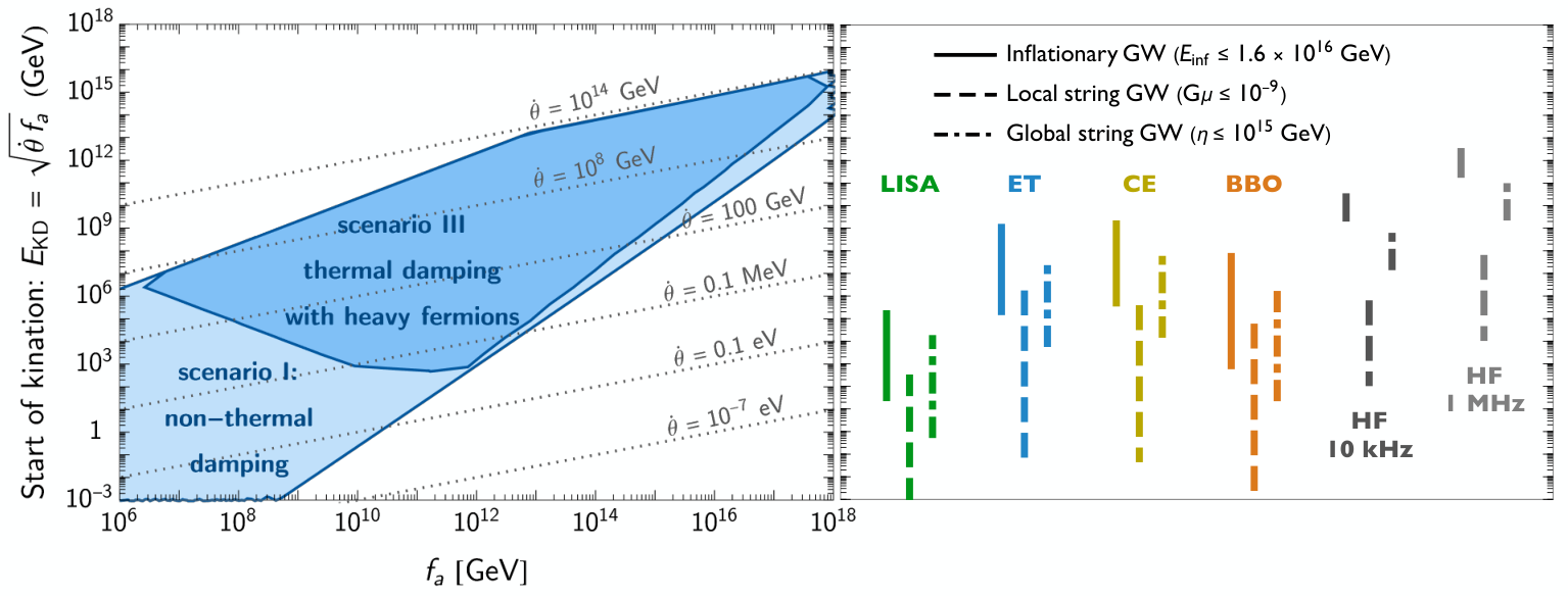
Model-independent
GW from primordial inflation
Fig. 7, 8
Eq. (3.12)
Eq. (3.13)
GW from local cosmic strings
Fig. 9, 10
Eq. (3.41)
Eq. (3.42)
GW from global cosmic strings
Fig. 11, 12
Eq. (3.48)
Eq. (3.50)
GW peak and axion relic abundance
Fig. 18, 19, 20
Eq. (4.10)
Eq. (4.22)
GW peak and baryon asymmetry
Fig. 21
Eq. (5.3)
Eq. (5.5)
Model-dependent
Model: radial mode + axion Fig. 24
Scenario I (non-thermal damping)
Fig. 31, 34, 36, 38
Eq. (7.37)
Scenario II (thermal damping) Fig. 39
Eq. (9.31)
Scenario III (thermal damping with non-relativistic fermions)
Fig. 42, 44, 45, 46, 47, 48
Eq. (7.38)
Acknowledgements
Special thanks go to our DESY colleagues Cem Eröncel, Pablo Quilez, Ryosuke Sato and Philip Sørensen for important discussions. We are also grateful to Hyungjin Kim, Enrico Morgante, Julián Rey, Pedro Schwaller, Ivan Sobolev, and Alexander Westphal. We thank Daniel Figueroa for his useful feedback during the DESY Theory Forum 2020 as well as Keisuke Harigaya and Kyohei Mukaida for clarifications and valuable insights on their papers. YG and GS are grateful to Galileo Galilei Institute for hospitality during the very final stage of this work while PS thanks Johannes Gutenberg Universität Mainz. YG acknowledges the Azrieli Foundation for the award of an Azrieli Fellowship. This work is supported by the Deutsche Forschungsgemeinschaft under Germany Excellence Strategy - EXC 2121 “Quantum Universe” - 390833306.
Appendix A Kination after inflation: quintessential inflation with -attractor
Kination has been discussed in the literature as a follow-up of inflation, and before reheating. While this paper instead investigates the possibility of kination inside the radiation era, except for the new constraints derived in Sec. 2.2, we review in this appendix motivations for models of kination following inflation for completeness. As already stated in Sec. 2.1, it is not possible to have a kination era from a canonical scalar field rolling down its potential without having superplanckian field excursions. On the other hand, kination arises in a popular class of inflation models called -attractor models which not only fit well CMB data but also link to quintessence at late time. In addition, they can be motivated in supergravity models. We summarise them in the following.
A.1 A sharp transition between two plateaus
-attractor.
-attractor is a class of supergravity theory where kinetic terms have poles
| (A.1) |
The use of -attractor for quintessential inflation has been studied in [218, 219, 220, 221, 222, 223]. Since the scalar field cannot cross the poles, the field range is limited to . For , it has the great advantage to prevent super-Planckian field excursion which plagues usual quintessential inflation scenarios.
Scalar potential.
Following [220, 221, 223], we choose the following scalar potential
| (A.2) |
where , which can be motivated by supergravity [224, 225], brane inflation [226], string theory [227, 228, 229] or gaugino condensation [230, 231, 232]. At late time, the scalar field slows downs when reaching an infinite kinetic term at . We suppose the existence of an unknown mechanism which set the cosmological constant (CC) to zero at
| (A.3) |
such that the scalar field potential energy + CC reads
| (A.4) |
Canonical normalization.
Upon introducing the field transformation
| (A.5) |
we obtain a canonically normalized scalar field with potential energy
| (A.6) |
A.2 Kination followed by reheating
Kination.
After inflation, the universe is dominated by the kinetic energy of the scalar field which evolves according to Eq. (2.1)
| (A.9) |
with the field position at the end of inflation estimated as
| (A.10) |
Since the inflation potential is non-oscillatory, the standard reheating can not occur through the decay of the inflaton.
Gravitational reheating.
The kination era ends when the universe becomes dominated by the energy density of the reheated plasma. An immediate possibility for producing radiation is gravitational reheating [44, 45] in which the reheated density reads
| (A.11) |
where is an efficiency factor which depends on the number of fields, the nature of their coupling with gravity, their mass and their self-coupling, see [62] for a review. However, unless we introduce a large number of self-interacting and/or non-minimally-coupled light fields, reheating through gravitational coupling only is inconsistent with the BBN bound on GW from inflation [13, 15, 233, 234, 235, 62].
Other reheating mechanisms.
A natural way-out, which may be the one realized in the SM [236], is to introduce a large non-minimal coupling to gravity to exploit the tachyonic instability generated by the change of sign of the Ricci scalar during kination [46, 47, 48, 49, 50]. The tachyonic instability can also be generated by a thermal phase transition [223] or more generally when the inflaton crosses an enhanced symmetry point, see instant reheating [237, 238, 221, 239] or trapping reheating [240, 241]. Another well-known efficient reheating is curvaton reheating where a spectator field decay into SM [242, 243, 244].
Appendix B Stiff-dominated era
B.1 Example of stiff era
The scalar Virial theorem, Eq. (G.41), states that the averaged energy density of the scalar field in the power-law potential, whose motion follows the Klein-Gordon equation in the expanding universe, redshifts as
| (B.1) |
which is equivalent to the EOS: .
B.2 BBN and interferometer probe
In Sec. 3.1, we have studied the spectrum of inflationary GW in presence of an arbitrary equation of state of the universe and we have found, see Eq. (3.9)
| (B.2) |
where is the equation of state of the universe. The energy-frequency relation is
| (B.3) |
where and are the GW frequency and the total energy density at the end of the stiff era. Examples of inflationary GW spectra in the presence of a stiff era are shown in Fig. 52-top. In Fig. 52-bottom, we show the reach of future-planned GW observatories. In contrast to the case shown in Fig. 2 where constraints from BBN were the strongest, here for and , the ability of GW interferometers to probe a stiff era can be better than what BBN does.


Appendix C Maximal duration of kination
In this appendix, we discuss what could lead to upper bounds on the number of e-folds of kination.
- 1.
- 2.
The constraint of kination-enhanced inflationary GW, cf. Eq. (C.2)
(C.3) - 3.
The growth of scalar fluctuation during kination, cf. Sec. C.3
(C.4) - 4.
- 5.
The universe contains a non-vanishing vacuum energy , cf. Sec. C.5,
(C.6)
We now derive these bounds in turn in the following subsections.
C.1 Duration between inflation/reheating and BBN
Maximal reheating scale.
The non-detection of primordial B modes by 2021 BICEP/Keck Collaboration [3] constrains the tensor-to-scalar ratio to be smaller than
| (C.7) |
where [245] and [246]. This implies the maximal Hubble and energy scale at the end of inflation to be
| (C.8) |
The maximum reheating scale, corresponding to the extreme scenario where reheating takes place instantaneously at the very end of inflation, is given by
| (C.9) |
Successful BBN.
By using the code AlterBBN [247], it can be shown ♠ ♠\spadesuit23 ♠ ♠\spadesuit23 23 We thank Philip Sørensen for this point. that successful BBN requires the amount of kination energy density to be less than of the radiation energy density at the temperature MeV [80]
| (C.10) |
We conclude that kination must end before
| (C.11) |
where is the energy scale at the end of kination when , and where we remind the reader of our notation . In the plots of our paper we actually use a slightly more aggressive constraint .
Maximal duration of kination after inflation (Scenario Type (i)).
Maximal duration of intermediate matter-kination (Scenario Type (ii)).
We consider the case of an intermediate matter-kination era, corresponding to Scenario Type (ii) in Fig. 1. As we already discussed along Eq. (2.16), the duration of the matter-kination is maximised when there is no entropy injection which would produce additional radiation component. For such an adiabatic evolution, the number of e-folds of matter and kination are related through
| (C.13) |
In that scenario the energy scale at the onset of the kination era is given by the geometric mean of the energy scales and at the onset of the matter era and at the end of the kination era
| (C.14) |
and the duration of the kination era alone can be written as
| (C.15) |
The longest matter-kination era allowed by CMB and BBN is the one which starts right after the end of inflation and ends just before the onset of BBN . We obtain the upper bound
| (C.16) |
The constraint can be seen in Fig. 31.
C.2 bound on inflationary GW
As we discuss in Sec. 2.2, the GW energy density produced prior to the onset of BBN can contribute to the effective number of neutrino species, which leads to the bound, cf. Eq. (2.6)
| (C.17) |
where [86], In Sec. 3.1, we have studied the impact of a kination EOS on the spectrum of primordial GW and we have found that a period of e-folds of kination leads to a blue-tilt whose peak value is, cf. Eq. (3.13)
| (C.18) |
Upon injecting Eq. (C.18) into Eq. (C.17), we obtain the maximal duration of kination
| (C.19) |
where Types (i) and (ii) are defined in Fig. 1. The constraint can be seen in Fig. 2.
C.3 Growth of scalar fluctuation
So far the strongest bound on the kination duration comes from the requirement of radiation era at the time of BBN. However, the scalar fluctuations in the early universe could lead to a stronger bound as the growth of fluctuation depends on the expansion history of the universe. For example, a long matter era can lead to a non-linear behavior of fluctuations [248, 249, 250] or the enhanced formation of primordial black holes [251]. Similarly, the fluctuations of the massless field which behave as radiation grow during kination era and could eventually dominate over that of the zero-mode which scales as stiff fluid after some efolds, determined by
| (C.20) |
where is the initial fluctuation’s energy density at the end of inflation. To estimate the bound on kination duration, one can assume that the growth is sourced by the curvature perturbations. The maximum energy density in the fluctuation would be the mode entering the horizon at the start of kination and could reach the level of the curvature perturbations observed in CMB . From this we can estimate that the number of e-folds of kination era is bounded to ♠ ♠\spadesuit24 ♠ ♠\spadesuit24 24 We thank Cem Eröncel for discussing this point.
| (C.21) |
This bound is further relaxed for less stiff era, e.g. for , respectively. We leave a more careful study of fluctuations during matter-kination era for future work [88]. We impose this constraint in Fig. 20.
C.4 Presence of axion wiggles
Assuming the presence of an axion potential
| (C.22) |
where is the mass of the axion . The circular motion of the angular mode is only possible if its kinetic energy density is larger than the energy density on the top of the potential barrier
| (C.23) |
Since the axion velocity redshift as , we deduce the maximal number of e-fold of kination
| (C.24) |
We obtained a similar bound from fragmentation in Eq. (4.38). We also checked that the early wiggles from higher-dimensional -explicit breaking terms do not lead to fragmentation.
C.5 Inflationary behavior after kination phase
Maximal number of kination e-folds.
So far, we have neglected the vacuum energy at the potential minimum. However, this non-zero potential energy can lead to an inflationary period at later times. The kinetic energy density redshifts as and eventually becomes as small as the vacuum energy
| (C.25) |
where is the e-foldings of the cosmic expansion after the kination era started. For a non-zero , Fig. 54 shows that after a number of kination e-folds given by
| (C.26) |
the EOS decreases abruptly to .
Physical motivations.
The vacuum-energy domination could signal a cosmological supercooled first-order phase transition about to take place.

Appendix D Origin of the scalar potential in the rotating complex scalar field model
The potential.
We consider a complex scalar field with the Lagrangian introduced in Eq. (7.1)
| (D.1) |
with the global -symmetric potential with spontaneous symmetry breaking (SSB) vacuum, the thermal corrections, the explicit -breaking term, and the Hubble-dependent potential
| (D.2) | ||||
| (D.3) | ||||
| (D.4) |
and
| (D.5) |
In this appendix, we derive the above scalar potential in SUSY framework. In the main text, we take .
D.1 Neglecting Hubble curvature
The first two terms, in Eq. (D.2) and Eq. (D.3), can be derived from the SUSY Lagrangian
| (D.6) |
with the Kahler potential and the superpotential being given by
| (D.7) | ||||
| (D.8) |
are the Grassmanian coordinates in the superspace. is the chiral superfield containing the complex scalar
| (D.9) |
is the messenger scale (e.g. the Planck scale for gravity mediation) and is a SUSY-breaking chiral superfield
| (D.10) |
which we assume to get a non-vanishing F-term VEV
| (D.11) |
where is the gravitino mass. From using Eq. (D.10), together with , the last two terms of the Kahler potential in Eq. (D.7) contribute to the scalar potential
| (D.12) |
while the second term of the Kahler potential in Eq. (D.7) acts as a non-holomorphic effective superpotential
| (D.13) |
and Eq. (D.8) can be replaced by
| (D.14) |
In turn, from the equations of motion for the F-terms of and
| (D.15) |
we obtain the scalar potential
| (D.16) |
From Eq. (D.12) and Eq. (D.16), we deduce and in Eq. (D.2) and Eq. (D.3)
| (D.17) | ||||
| (D.18) |
with
| (D.19) | ||||
| (D.20) |
The quartic term in Eq. (D.12) is negligible as long as . The presence of the logarithmic function in Eq. (D.17), which is responsible for the spontaneous breaking of the symmetry , is generated radiatively [192], see App. D.4 for a review. The constant term in the same equation is needed in order to tune the cosmological constant to zero.
D.2 Including Hubble expansion
Let’s assume that the energy density is dominated by a complex scalar , which can be the inflaton during inflation or matter-dominated preheating [210, 211] or a field in equilibrium with the thermal plasma during radiation domination [252]
| (D.21) |
where is the F-term of the chiral superpotential containing . Our complex scalar of interest , which is a sub-dominant fraction of the energy density of the universe , interacts with through gravity, which leads to the non-renormalizable Kahler potential
| (D.22) |
Upon solving for the -F-term equations of motion from the total Lagrangian Eq. (D.7), (D.8) and Eq. (D.22), in which we replace ♠ ♠\spadesuit25 ♠ ♠\spadesuit25 25 We remind the reader that chiral superfields in superspace read with , which implies . In Eq. (D.23), we have neglected the fermionic component , the inflaton VEV and the mass term .
| (D.23) |
we find that the scalar potential receives the additional terms
| (D.24) |
If the dynamics occurs during radiation-domination, then dominates and the scalar potential receives a negative curvature-induced mass whenever
| (D.25) |
If the dynamics occurs during inflation or matter-domination, then dominates ♠ ♠\spadesuit26 ♠ ♠\spadesuit26 26 The term in Eq. (D.26) is generated by the interaction between the three non trivial terms , and in the Kahler potential.
| (D.26) |
with defined in Eq. (D.20). The Hubble-induced mass is negative whenever and . For , the latter condition is verified whenever the SUSY-breaking field does not dominate the energy density of the universe . We refer to [210, 211] for a discussion of supergravity corrections, which should become important during inflation whenever .
In summary, we see that a large and negative Hubble-induced mass term is naturally generated in models where the complex scalar field couples to a field that dominates the energy density of the universe. This is very important for justifying the initial conditions.
D.3 Evolution of the scalar field in the negative Hubble-induced potential.
Damped harmonic oscillator.
We recall the damped harmonic oscillator
| (D.27) |
has three regimes according to the value of
| (D.28) |
where are constants set by the initial conditions. Taking and introducing , we obtain, e.g. [212]
| (D.29) |
Initial radial value.
Neglecting the -breaking term and assuming in Eq. (D.26), the potential at early time reads, cf. Eq. (D.17), Eq. (D.18) and Eq. (D.26)
| (D.30) |
where we included a thermal mass coming from a possible interaction with the thermal bath. We study the dynamics of the scalar field at early time by numerically integrating the field equation of motion in the presence of the potential in Eq. (D.30). In order to simplify the numerical study, we assume that the universe is radiation-dominated, so that the temperature is related to the Hubble parameter through
| (D.31) |
From Eq. (D.29), we deduce that there are three stages of field evolution after which the field starts oscillating with an amplitude in a potential with minimum . ♠ ♠\spadesuit27 ♠ ♠\spadesuit27 27 At early stage, we can forget about the existence of the SSB minimum at . The resulting field trajectory is plotted in Fig. 55.
- 1.
: the negative Hubble-mass dominates the mass term so the fields rolls within e-folds towards the non-trivial minimum at
(D.32) - 2.
: the Hubble-mass becomes sub-dominant and the time-dependent minimum vanishes .
- 3.
: the Hubble friction drops, the field becomes under-damped, , and starts to roll away from
(D.33)

The trajectories shown in Fig. (55) assume that the dynamics occurs during a radiation-dominated era. If the Hubble-induced mass is generated from the inflaton sector, the Hubble-induced mass decreases instead during preheating and the field starts rolling away from the non trivial value in Eq. (D.33) as soon as drops below .
Initial angle.
For F-term dominated universe, cf. Eq. (D.26), the breaking term receives Hubble-dependent corrections
| (D.34) |
Therefore, the positions of the valleys of minimum potential are time dependent. The same dynamics, just described above for the radial mode, also applies for the angular mode. The angular field rolls towards a temporary vallee during inflation when , and starts rolling towards the Hubble-independent valley when drops below . In this work, we simply assume the initial angular amplitude ♠ ♠\spadesuit28 ♠ ♠\spadesuit28 28 Note that for radiation-dominated universe, the A-term in Eq. (D.24), at least in our analysis and in the ones of [196, 216], seems to be Hubble-independent. We leave for further study the question of whether such Hubble-dependent A-term is induced during radiation-domination. In any case, the angular kick could be generated by random fluctuations during inflation, see Sec. 7.5.2.
| (D.35) |
D.4 Nearly-quadratic potentials
In this appendix, we review the results presented in [192] which show how spontaneous symmetry breaking can arise due to the running of the soft masses. The authors consider supersymmetric theories coupled to supergravity where is a global symmetry of the superpotential. They show that can be broken by the logarithmic running of renormalization group equations. Their results are not specific of the Peccei-Quinn symmetry and they can be generalized to other global .
Introduce chiral superfields.
The superpotential is given by
| (D.36) |
where the quantum numbers of the chiral superfields are
| (D.37) |
and are singlets under . The fields transform under the as
| (D.38) |
There is a continuum of supersymmetric minima
| (D.39) |
SUGRA breaking.
Supergravity couplings lift this flat direction by inducing soft supersymmetric breaking terms characterized by the gravitino mass
| (D.40) |
The initial conditions for the RGE are set at the Planck scale ,
| (D.41) |
The effective scalar potential is
| (D.42) |
and along the supersymmetric minimum , it is reduced to
| (D.43) |
Renormalization group equations.
Loop corrections to the couplings lead to the running [192]
| (D.44) | ||||
| (D.45) | ||||
| (D.46) | ||||
| (D.47) |
where and is the gauge-coupling of the . The equation for can be solved analytically with
| (D.48) |
All the couplings are related , hence we have
| (D.49) |
The system of first-order differential equations above has a fixed point at
| (D.50) |
where is running as
| (D.51) |
and is approximately constant.
Dimensional transmutation.
In the limit , the above equation is solved analytically by
| (D.52) |
where the approximation is used. Then we define scale by when the radiative correction changes the sign of effective potential, i.e. at
| (D.53) |
where is related to by
| (D.54) |
With the definition of , the coupling is simplified to
| (D.55) |
The effective potential.
The effective potential reads
| (D.56) |
For and , we have .
Appendix E Inflationary fluctuations in the rotating complex scalar field model
E.1 Adiabatic curvature perturbations
Any light scalar present during inflation receives quantum fluctuations which classicalize upon horizon exit, e.g. [253]. When such perturbations re-enter the horizon, they source either the adiabatic or the isocurvature power spectrum according to whether the extra specie thermalizes with the SM or not. In our model, cf. Sec. 7, the radial mode of the complex scalar field decays into thermal radiation and therefore contributes to the adiabatic part of the curvature perturbations. Assuming a quadratic scalar potential with , the perturbation from the decaying scalar field reads [254]
| (E.1) |
where is the energy density fraction carried by the scalar, evaluated at the time of radial damping. The upper bound on corresponds to the value measured by CMB [2]
| (E.2) |
To constrain the model, we consider two limits.
1) Damping before domination. Assuming the extreme case in which radial damping occurs right after the onset of radial mode oscillation, c.f. Eq. (7.29), in order to minimize , the adiabatic curvature power spectrum reads
| (E.3) |
where is the value at oscillation.
- •
- •
If the initial field value is driven by the negative-Hubble mass and is stabilized by higher-order terms, the quantum fluctuation of the radial and angular fluctuation are suppressed, see Sec. E.4. This is the scenario which we assume in this paper.
2) Damping when dominating. Assuming in Eq. (E.1) leads to and to the adiabatic curvature perturbations
- •
- •
As mentioned in the previous paragraph and as we will discuss more precisely in Sec. E.4, for scenarios with Hubble-size masses, quantum fluctuations are suppressed and the Planck constraints are avoided.

E.2 Domain wall problem
Quantum fluctuations of the initial angular phase , and of the initial radial value lead to a fluctuation of the final angular phase at the time when the axion potential develops. This can lead to the formation of domain walls (DW). In the absence of CS, e.g. in the pre-inflationary PQ-breaking scenario, the DW are infinite and can not decay, so we must impose .
Assuming , from charge conservation in Eq. (7.19) and from the scaling in Eq.(G.41), we deduce the scaling of the angular velocity
| (E.6) |
where we assume a radiation-dominated universe. The angular phase elapsed after the onset of radial mode oscillation which we denote by reads
| (E.7) |
The fluctuation in the angular phase can be written as
| (E.8) |
From Eq. (G.9), and Eq. (7.5), we can write
| (E.9) |
The late time phase fluctuation in Eq. (E.8) becomes
| (E.10) |
where the last term in the squared bracket dominates for and . Plugging the typical standard deviation for a massless field during inflation, e.g. [253]
| (E.11) |
we obtain the necessary condition for preventing DW formation once the axion potential switches on
| (E.12) |
where we replaced . The flatter the potential, the slower the redshift of the angular velocity and the larger the final time fluctuation .
E.3 Isocurvature perturbations
If the axion contributes to the DM abundance then the quantum fluctuation during inflation in Eq. (E.11) generate isocurvature perturbations [255, 256, 257, 258] ♠ ♠\spadesuit29 ♠ ♠\spadesuit29 29 This problem also arises in the context of the Affleck-Dine Baryogenesis, where the inflationary perturbation leads to the baryonic isocurvature perturbations [259, 260, 261, 262, 263]. whose amplitude is bounded by Planck data [2]
| (E.13) |
For a spinning axion, the axion abundance is set by the kinetic misalignment mechanism , cf. Eq. (4.9). From Eq. (E.9) and Eq. (E.11), we deduce
| (E.14) |
where .
E.4 Solution
A way to cure the three problems listed above - too large adiabatic and isocurvature perturbations and DW overclosure - is to suppress the initial quantum fluctuations by introducing a large mass for both the radial mode and the angular mode , during inflation [264, 265, 266, 267, 263, 268, 180].
As discussed along Eq. (7.25), Hubble size masses for and arise naturally in SUSY scenario where we have
| (E.15) |
So, in fact, the solution to these problems is built-in in these models. Quantum fluctuations of massive states are blue-tilted, e.g. [253], such that the amplitude of the associated curvature perturbations entering the Hubble horizon long after the end of inflation, are expected to be negligible. This is the scenario which we consider in this paper and therefore we assume that the initial field value is set by the classical minimum of the Hubble-induced SUSY potential in Sec. 7.5.1 and not by the Bunch-Davies quantum distribution in Sec. 7.5.2.
Appendix F Damping of the radial motion in the rotating complex scalar field model
F.1 Thermalization
Fermion portal.
We assume that the complex scalar field is coupled to heavy fermions charged under some (hidden or SM) gauge sector (KSVZ-type interactions)
| (F.1) |
At zero temperature, the scalar condensate decays into fermions pairs with a rate, cf. diagram in Fig. 57
| (F.2) |
If the fermion mass, either from vacuum or thermal origin , is larger than the scalar field mass, then the scalar field cannot excite thermal and it is dominantly depleted through scattering with thermally-dressed fermions of the plasma, cf. diagram in Fig. 57, with a rate [193, 194]
| (F.3) |
The two regimes in Eq. (F.3) depend on whether the thermal width - the typical relaxation rate of the fermion density towards thermal equilibrium - is larger or smaller than the fermion zero-temperature mass . If the temperature is smaller than the fermion mass, , the heavy fermions are absent of the thermal plasma. In that case, the scalar field can decay into gauge bosons through a loop of fermions [195, 197, 198], cf. diagram in Fig. 57
| (F.4) |
For , we replace in Eq. (F.4) by . The dependence on in Eq. (F.4) appears in the logarithmic running of . So we conclude
| (F.5) |

The scalar field keeps spinning after thermalization.
The coherent oscillation is a very ordered state and once the oscillation energy begins to be transferred into the thermal bath, the inverse process which creates coherent oscillation is unlikely to occur. Therefore, the thermalization of the scalar field, when the universe reaches the energy density
| (F.6) |
transfers all the kinetic energy of the radial mode to the plasma . The kinetic energy of the angular mode, aka the charge, can also be transferred to the thermal bath, e.g. in the form of chiral charges of SM fermions. However, as shown by the supplementary material of [38], the creation of an asymmetric fermion abundance costs chemical potential which leads to an energy density and it turns out that it is thermodynamically favorable to keep the charge in the condensate with energy density as long as
| (F.7) |
where is the temperature when reaches . We check that this condition is satisfied in Eq. (10.24). The washout of charge due to chirality flip mediated by Yukawa interactions is shown to be negligible if the temperature of thermalization is smaller than [38]
| (F.8) |
Using that the scalar field evolves in its quadratic potential as
| (F.9) |
we obtain that the axion rotation is preserved from wash-out from the onset of oscillation until the final stage as long as
| (F.10) |
The later condition is largely satisfied in the parameter space of our interest, and wash-out never occurs.
Thermal corrections to the potential.
The presence of the interactions in Eq. (F.1) generates thermal corrections to the scalar potential [193, 194]
| (F.11) | ||||
| (F.12) |
The first Heaviside function stands for the Boltzmann suppression of the fermion abundance in the thermal plasma in the large vev limit . In that case the thermal corrections are given by the thermal-log potential, obtained after integrating out the heavy fermions [195, 199, 197, 198]. At small vev value , the running of the gauge coupling constant becomes independent of , which explains the second Heaviside function.
Impossibility to generate efficient thermalization when neglecting thermal corrections.
Let’s first assume that thermal corrections to the potential in Eq. (F.12) do not impact the scalar field dynamics. This happens whenever the thermal mass of the scalar fields can be neglected at the time of oscillation , see Eq. (8.1), ♠ ♠\spadesuit30 ♠ ♠\spadesuit30 30 We backward check that this coincides with (the first Heaviside function in Eq. (F.12)) whenever the initial field value is sub-planckian (F.13)
| (F.14) |
The duration of the kination era reads, cf. Sec. 8.2
| (F.15) |
with
| (F.16) |
From plugging ♠ ♠\spadesuit31 ♠ ♠\spadesuit31 31 We checked that implies and , leading to in Eq. (F.5). , cf. Eq. (F.5), , which corresponds to the limit of Eq. (7.28) and , cf. Eq. (F.14) we obtain
| (F.17) |
So we conclude that whenever the conditions of neglecting the thermal mass in Eq. (F.14) is satisfied, thermalization via fermion portal is not efficient enough to generate a kination era.
For this reason, in scenario I of Sec. 8, we must postulate the existence of an unknown mechanism, other than thermalization via fermion or Higgs portal, to damp the radial mode.
The effects from the thermal mass are considered in scenario II of Sec. 9. Unfortunately, the suppression of the angular kick and the delay of the matter domination prevents the onset of kination.
In scenario III in Sec. 10, instead of choosing a low Yukawa coupling , we get rid of the thermal effects at the onset of the radial mode oscillation by Boltzmann-suppressing the fermion abundance.
Higgs portal.
In the previous paragraph, we have considered the fermion portal. If instead the scalar condensate thermalizes through a Higgs mixing (DFSZ-type interactions)
| (F.18) |
The thermal mass correction to the condensate is
| (F.19) |
The quantum processes responsible for the thermalization of the condensate are described in [270]. In contrast to the fermion portal (denoted by ), in the case of the Higgs portal (denoted by ) the thermalization rates scale as the the forth power of the thermal mass. Indeed
| (F.20) |
with
| (F.21) |
We conclude that the situation of the previous paragraph - to impose a small thermal mass prevents thermalization to occur before the start of the would-be kination era - is even worse in the case of the Higgs portal.
F.2 Parametric resonance
In this paper we focus on the zero-mode dynamics. However, there may be circumstances where higher modes get produced. We now introduce the framework to study early parametric resonance, which may occur in the UV completion and may have important consequences on the whole dynamics. The equation of motion of a complex scalar reads
| (F.22) |
which after decomposing in polar coordinates , becomes
| (F.23) | ||||
| (F.24) |
We can decompose into the superposition of a classical homogeneous mode and small fluctuations around it
| (F.25) | ||||
| (F.26) |
with , being the annihilation and creation operators of field
| (F.27) |
and the initial condition for the mode function at is given by
| (F.28) |
We now treat as perturbations. We expand the potential around the background solution
| (F.29) |
such that after spatial and quantum averaging we get, e.g. [39, 150, 271].
| (F.30) | ||||
| (F.31) |
for the zero mode, and
| (F.32) | ||||
| (F.33) |
for the higher modes, where
| (F.34) |
Since , all the quantum average of cross terms in Eq. (F.30) and (F.31) vanish and we get
| (F.35) | ||||
| (F.36) |
We conclude that the Noether charge
| (F.37) |
is conserved during parametric resonance. Note that from using Eq. (F.36), Eq. (F.33) simplifies to [271]
| (F.38) |
In order to address the question of whether parametric resonance is a successful mechanism for damping the radial mode or not - an important question for scenario I in Sec. 8 - we need to solve the system of Eqs. (F.32), (F.33), (F.35) and (F.36). We leave this question for further study.
Appendix G Detailed solution of field evolution in the rotating complex scalar field model
G.1 The angular kick
The angular EOM, Eq. (7.17), can be rewritten as a Boltzmann equation for the charge
| (G.1) |
which is equivalent to
| (G.2) |
This equation suggests that the charge production rate is proportional to the potential gradient in the angular direction. Numerical simulations plotted in Fig. 26 show that the charge generation can possibly start even before that the field starts to roll in the radial direction at . Once the field value drops substantially, the explicit breaking term becomes negligible, see Fig. 58, and the charge becomes conserved.
We can determine the angular kick by integrating Eq. (G.2)
| (G.3) |
where is the scale factor of the universe in the far past, where we plugged the explicit breaking potential in Eq. (D.3). The production rate of the charge behaves differently accordingly to whether the radial mode has started rolling , or not.
- •
Before oscillation: the field initially stands at , see Sec. 7.5. Assuming the universe is dominated by the background energy density , the corresponding charge generation is
(G.4) (G.5) (G.6) where we approximate and take it out of the integration. The late-time contribution dominates the charge generation such that we have the charge evolution
(G.7) and we see that the field receives a kick even before the time of oscillation with . The charge is maximally generated at the onset of oscillation
(G.8) and the corresponding angular velocity reads
(G.9) - •
After the oscillation: gradients of the potential in angular and radial directions kick the field into an elliptic orbit whose size redshifts over time. In App. G.2, we determine the dynamics of the radial mode as a function of the shape of the -symmetric potential
(G.10) Assuming that the Hubble factor evolves as , then the charge generated after oscillation , in Eq. (G.3), reads
(G.11) Depending on the values of , , and , we obtain three regimes
(G.12) In the first and second cases, the charge continues to increase after the oscillation, while in the third case at large , the charge stops being efficiently produced after a few Hubble times and the -symmetry is restored. Assuming a radiation-dominated universe (), the estimated -symmetry after the oscillation demands that is greater than and for quadratic () and quartic () potentials, respectively. Hence, in this work we consider cases in order to neglect explicit breaking terms at later time.
G.2 After the kick
The -conserving and the -breaking potentials excite the field in the radial and angular directions, respectively. As argued in App. G.1, after a few Hubble times of field evolution, for we can neglect effects coming from the -breaking terms.
Exact solution.
We now derive an exact analytical solution of the complex scalar equation of motion in a quadratic potential without Hubble friction, e.g. [272, 273]. For , the nearly-quadratic potential in Eq. (7.4) is approximated to , where is a constant or a slowly-changing variable. The -charge conservation in Eq. (7.19), and the radial EOM in Eq. (7.16), give
| (G.13) |
where is the conserved comoving charge. We use a set of dimensionless parameters
| (G.14) |
which simplifies the charge conservation equation to and the EOM to
| (G.15) |
where denotes the derivative w.r.t. , and where we considered the oscillation time scale to be much faster than a Hubble time , which becomes true after oscillation has started . The differential equation in Eq. (G.15) can be understood as the equation of motion of a scalar evolving in a potential
| (G.16) |
whose minimum is at , or equivalently . Its corresponding constant-of-motion satisfies
| (G.17) |
with . The parameter can be related to the energy density of the scalar field
| (G.18) |
We just found that the energy density of a complex scalar field evolving in a quadratic potential, redshifts as matter .
To find the exact solution to the EOM, we rewrite Eq. (G.17) as
| (G.19) |
where . Integrating this equation, we deduce
| (G.20) |
where is a phase which depends on the initial conditions. In -space, the orbit is a fixed-sized ellipse, so the orbit in field space is an ellipse whose size scale as , i.e. an ellipse that spirals towards the origin as illustrated in Fig. 24 or by our animation.. The parameter is related to the orbit eccentricity and to the previously defined parameter in Eq. (8.3)
| (G.21) |
For or , the orbit is essentially circular, while for large or the orbit has a large eccentricity and starts to resemble the trajectory of a real scalar field.
We can calculate the average angular speed
| (G.22) |
by averaging over a time , , which is larger than the oscillation period but less than the Hubble time scale
| (G.23) |
where we have integrated an elliptic integral ♠ ♠\spadesuit32 ♠ ♠\spadesuit32 32 We can freely choose the phase such that the sine becomes a cosine and the elliptic integral reads . We find that the averaged angular velocities becomes independent of the initial value in Eq. (G.9) and converges towards an attractor solution. This is confirmed by the numerical integration of the equations of motion in Fig. 26.
Exact solution (bis) : quartic potential.
Even if we don’t use it in our work, it may be useful for further studies (of axion dark matter for example [80]) to give the analog of Eq. (G.20) for a quartic potential. When adding a quartic term to the potential , the Eq. (G.15) becomes
| (G.24) |
We now consider , such that the linear term corresponding to can be dropped and Eq. (G.24) becomes
| (G.25) |
with and with ′ denoting the derivative with respect to the conformal time ( ) and where we have dropped Hubble depending terms. The motion can be interpreted as a scalar oscillating in a potential with the constant of motion Introducing the new variables and , we deduce
| (G.26) |
It is known that the Weierstrass elliptic function solves the differential equation of the form [274]
| (G.27) |
Therefore, Eq. (G.26) has a solution as an elliptic orbit described by . Applying one of the properties of , namely the exact solution to Eq. (G.25) reads
| (G.28) |
Virial theorem.
The Virial theorem in classical mechanics is a well-known tool, e.g. [275], for studying the averaged behavior of a stable system. We now use it to study the dynamics of a complex scalar field in a central potential during the early universe. The EOM in Eq. (7.16) and (7.17) can be written in terms of kinetic and potential energy densities as
| (G.29) | ||||
| (G.30) | ||||
| (G.31) |
where and are the kinetic energy in radial and angular modes, respectively. After , the field oscillates fast compared to the expansion and damping rate. The average over many field cycles but over a time shorter than the reads
| (G.32) |
We introduce the Virial parameter , e.g. [275]
| (G.33) |
where and , and . By taking its time derivative, we deduce
| (G.34) | ||||
| (G.35) | ||||
| (G.36) |
where we used Eq. (7.16) and (7.17) in the second step, and where we neglected the damping terms in the last step. The Virial theorem states that whenever the system is stable, the averaged kinetic and potential energies are related
| (G.37) |
which resembles the Virial theorem for a real scalar [193, 194]. For convenience, we consider the field behavior before the damping term becomes effective and deduces the average EOM from Eq. (G.32) and (G.37)
| (G.38) |
Monomial potential.
From plugging the potential into Eq. (G.38), we obtain
| (G.39) |
with is the average total energy density of the field
| (G.40) |
We deduce the redshift laws of and
| (G.41) |
For the quadratic and quartic potentials, the complex scalar field behaves like matter (, ) and radiation (, ), respectively. The scaling is confirmed by the exact solution in Eq. (G.18). We show that, cf. Eq. (G.54), that Eq. (G.39) holds without any average after radial damping .
Thermal mass.
From plugging the potential into Eq. (G.38), we obtain
| (G.42) |
We conclude that in a radiation-dominated universe, a scalar field dominated by its thermal mass redshifts like radiation.
G.3 The radial damping
Amount of rotation.
The parameter expresses the amount of rotation generated by the explicit breaking at the time of oscillation , cf. Eq. (8.3)
| (G.43) |
From Eq. (8.9), we deduce that becomes a conserved quantity through Hubble expansion , as soon as become dominated by its quadratic term. It can be rewritten in terms of the ratio between energy densities as
| (G.44) |
Since , see Fig. 26, we deduce the rotational energy density to be an fraction of the potential energy density
| (G.45) |
Note that from preventing the field to spin upward.
| (G.46) |
Drop of energy density during radial damping.
During the radial damping , see Sec. 7.6, the elliptic orbits becomes a circular one. During this process, the scalar field kinetic energy is damped but the rotational kinetic energy is preserved. Therefore, after the radial damping the total energy density of the complex scalar field drops by
| (G.47) |
where the second equation assumes the quadratic potential. is the field value just before thermalization, and it can be computed from Eq. (G.41)
| (G.48) |
where we used that the energy density just after oscillation can be written as . In Fig. 59, we show that the result in Eq.(G.47) is confirmed by numerical integration of the equations of motion.


Impact on kination duration.
We now study the impact of the energy drop in Eq. (G.47) on the duration of the kination era. As shown in Fig. 27, we must consider two possible scenarios, depending on whether the radial damping occurs before or after the scalar domination. For the sake of simplicity we assume an instantaneous drop in energy density at the time of radial damping.
- •
Damping before domination. The energy transferred to the thermal bath is negligible. However, the factor in the energy density in Eq. (G.47) delays the time when the scalar field dominates the energy density of the universe
(G.49) where is the domination energy scale without energy drop during damping (case ) and where we have used Eq. (G.79).
As a consequence of the energy drop, the kination era ends earlier and is then shorter
(G.50) - •
Damping after domination. A substantial amount of energy is injected in the thermal bath. For , the radial damping reduces the scalar energy by a factor , so that the produced SM radiation dominates the energy density. Later, the domination of the energy density by the rotating scalar generates a second matter era at
(G.51) The scale of kination ending and its duration are given by Eq. (G.50) after replacing by
(G.52) Note that the presence of the radiation era in between the two matter eras could leave a distinctive imprint in the SGWB.
Too small kills the kination era.
In Eqs. (G.50) and (G.52), we have seen that the kination duration receives a suppression factor . This implies the existence of a lower bound on below which no kination era is generated
| (G.53) |
for both damping before and after the scalar domination. In Sec. 9, we show that the scenario II, in which thermal corrections to the potential are present at the onset of the radial mode oscillation, necessarily predicts a value of smaller than Eq. (G.53).
G.4 After the radial damping
In this section, we reproduce the results from [38] and derive the evolution of the radial and angular field values, their energy density and equation of state , in an arbitrary -symmetric potential , after that the radial mode has been damped .
Radial evolution.
In the limit , the radial EOM in Eq. (7.16) takes a simple form
| (G.54) |
We inject it in the equation of conservation of
| (G.55) | ||||
| (G.56) | ||||
| (G.57) |
From which we obtain
| (G.58) |
Angular evolution.
Energy density evolution.
After radial damping, the kinetic energy of the radial mode vanishes such that the energy density of the complex field reads
| (G.60) |
Taking the derivative with respect to , we get
| (G.61) |
Now taking the derivative with respect to
| (G.62) |
where is the kinetic energy density of the angular field
| (G.63) |
we deduce
| (G.64) |
Equation of state.
Example: Nearly-quadratic potential.
This is the scenario considered in this work. The potential and its derivatives read ♠ ♠\spadesuit34 ♠ ♠\spadesuit34 34 Note that is the minimum of potential is not vanishing , then the evolution of the energy density and EOS becomes (G.67) In order to generated a kination EOS, in this work we assume .
| (G.68) |
From using Eq. (G.58) and (G.59), we deduce the evolution of the radial and angular component of the scalar field after radial damping
| (G.69) |
Using Eq. (G.64) and (G.66), we deduce the evolution of the complex scalar field energy density and its equation of state
| (G.70) |
For we have
| (G.71) |
and for we have
| (G.72) |
Example: quartic potential.
For the sake of the comparison, we consider the potential
| (G.73) |
Eq. (G.58) and (G.59) From using Eq. (G.58) and (G.59), we deduce the evolution of the radial and angular component of the scalar field after radial damping
| (G.74) |
Using Eq. (G.64) and (G.66), we deduce the evolution of the complex scalar field energy density and equation of state
| (G.75) |
For we have
| (G.76) |
and for we have
| (G.77) |
The evolution of and in nearly-quadratic and quartic potentials are shown in Fig. 60. Only the matter phase induced by the nearly-quadratic potential can allow the initially sub-dominant to dominate the energy density of the universe and, later, generate a kination-dominated era. For this reason, in this work we focus on a nearly-quadratic potential. In Fig. 28, we show the evolution of , , and in the nearly-quadratic potential, obtained after numerically integrating the equations of motion in Eqs. (7.16), (7.17) and (7.18).
G.5 Derivation of the cosmological-history relations
In this appendix, we derive the expression used in Sec. 8.2, neglecting the factor , and for which we refer to App. G.3.
Matter domination.
After the field starts oscillating at , it redshifts like matter and induces a matter-domination era as soon as it dominates the energy density of the universe when
| (G.78) |
where we have neglected the change of relativistic degrees of freedom in the thermal bath. We obtain
| (G.79) |
Radial damping.
The decay of the radial mode, occuring at the rate , dissipates the radial kinetic energy when
| (G.80) |
after that the universe has expanded by
| (G.81) |
Start of kination (starting).
The scalar field reaches the kination-liked equation of state when the radial field-value settles down to its final VEV , when the energy density is
| (G.82) |
where the radial kinetic energy vanishes after and where we assume the vacuum energy to vanish at the minimum. The duration of the matter era reads
| (G.83) |
End of kination.
The period of kination lasts until the energy density of the scalar field drops below that of thermal bath. The value of the radiation energy density depends on whether entropy has been injected during the damping of the radial mode. This depends on whether radial damping has occured after domination , or not. Its energy density at the end of kination era follows the scaling law
| (G.84) |
Similarly, the scalar field which has undergone a period of matter folowed by a period of kination has the energy density
| (G.85) |
From the above two equations, we deduce the energy density at the end of kination
| (G.86) |
and the duration of the kination era
| (G.87) |
References
- [1] BICEP2, Keck Array collaboration, P. Ade et al., BICEP2 / Keck Array x: Constraints on Primordial Gravitational Waves using Planck, WMAP, and New BICEP2/Keck Observations through the 2015 Season, Phys. Rev. Lett. 121 (2018) 221301, [1810.05216].
- [2] Planck collaboration, Y. Akrami et al., Planck 2018 results. X. Constraints on inflation, Astron. Astrophys. 641 (2020) A10, [1807.06211].
- [3] BICEP, Keck collaboration, P. A. R. Ade et al., Improved Constraints on Primordial Gravitational Waves using Planck, WMAP, and BICEP/Keck Observations through the 2018 Observing Season, Phys. Rev. Lett. 127 (2021) 151301, [2110.00483].
- [4] R. Allahverdi et al., The First Three Seconds: a Review of Possible Expansion Histories of the Early Universe, 2006.16182.
- [5] B. Spokoiny, Deflationary universe scenario, Phys. Lett. B 315 (1993) 40–45, [gr-qc/9306008].
- [6] M. Joyce, Electroweak Baryogenesis and the Expansion Rate of the Universe, Phys. Rev. D 55 (1997) 1875–1878, [hep-ph/9606223].
- [7] P. G. Ferreira and M. Joyce, Cosmology with a primordial scaling field, Phys. Rev. D 58 (1998) 023503, [astro-ph/9711102].
- [8] M. Joyce, Habilitation thesis, 2001.
- [9] C. Caprini and D. G. Figueroa, Cosmological Backgrounds of Gravitational Waves, Class. Quant. Grav. 35 (2018) 163001, [1801.04268].
- [10] M. Giovannini, Gravitational waves constraints on postinflationary phases stiffer than radiation, Phys. Rev. D58 (1998) 083504, [hep-ph/9806329].
- [11] M. Giovannini, Stochastic backgrounds of relic gravitons: a theoretical appraisal, PMC Phys. A 4 (2010) 1, [0901.3026].
- [12] A. Riazuelo and J.-P. Uzan, Quintessence and gravitational waves, Phys. Rev. D62 (2000) 083506, [astro-ph/0004156].
- [13] V. Sahni, M. Sami and T. Souradeep, Relic gravity waves from brane world inflation, Phys. Rev. D65 (2002) 023518, [gr-qc/0105121].
- [14] N. Seto and J. Yokoyama, Probing the equation of state of the early universe with a space laser interferometer, J. Phys. Soc. Jap. 72 (2003) 3082–3086, [gr-qc/0305096].
- [15] H. Tashiro, T. Chiba and M. Sasaki, Reheating after quintessential inflation and gravitational waves, Class. Quant. Grav. 21 (2004) 1761–1772, [gr-qc/0307068].
- [16] K. Nakayama, S. Saito, Y. Suwa and J. Yokoyama, Space laser interferometers can determine the thermal history of the early Universe, Phys. Rev. D77 (2008) 124001, [0802.2452].
- [17] K. Nakayama, S. Saito, Y. Suwa and J. Yokoyama, Probing reheating temperature of the universe with gravitational wave background, JCAP 06 (2008) 020, [0804.1827].
- [18] R. Durrer and J. Hasenkamp, Testing Superstring Theories with Gravitational Waves, Phys. Rev. D 84 (2011) 064027, [1105.5283].
- [19] S. Kuroyanagi, K. Nakayama and S. Saito, Prospects for determination of thermal history after inflation with future gravitational wave detectors, Phys. Rev. D84 (2011) 123513, [1110.4169].
- [20] S. Kuroyanagi, T. Chiba and T. Takahashi, Probing the Universe through the Stochastic Gravitational Wave Background, JCAP 1811 (2018) 038, [1807.00786].
- [21] R. Jinno, T. Moroi and K. Nakayama, Probing dark radiation with inflationary gravitational waves, Phys. Rev. D86 (2012) 123502, [1208.0184].
- [22] P. D. Lasky et al., Gravitational-wave cosmology across 29 decades in frequency, Phys. Rev. X6 (2016) 011035, [1511.05994].
- [23] B. Li, P. R. Shapiro and T. Rindler-Daller, Bose-Einstein-condensed scalar field dark matter and the gravitational wave background from inflation: new cosmological constraints and its detectability by LIGO, Phys. Rev. D96 (2017) 063505, [1611.07961].
- [24] K. Saikawa and S. Shirai, Primordial gravitational waves, precisely: The role of thermodynamics in the Standard Model, JCAP 05 (2018) 035, [1803.01038].
- [25] R. R. Caldwell, T. L. Smith and D. G. E. Walker, Using a Primordial Gravitational Wave Background to Illuminate New Physics, 1812.07577.
- [26] N. Bernal and F. Hajkarim, Primordial Gravitational Waves in Non-standard Cosmologies, 1905.10410.
- [27] D. G. Figueroa and E. H. Tanin, Ability of LIGO and LISA to probe the equation of state of the early Universe, JCAP 08 (2019) 011, [1905.11960].
- [28] F. D’Eramo and K. Schmitz, Imprint of a scalar era on the primordial spectrum of gravitational waves, Phys. Rev. Research. 1 (2019) 013010, [1904.07870].
- [29] B. Li, T. Rindler-Daller and P. R. Shapiro, Cosmological Constraints on Bose-Einstein-Condensed Scalar Field Dark Matter, Phys. Rev. D 89 (2014) 083536, [1310.6061].
- [30] B. Li and P. R. Shapiro, Precision cosmology and the stiff-amplified gravitational-wave background from inflation: NANOGrav, Advanced LIGO-Virgo and the Hubble tension, JCAP 10 (2021) 024, [2107.12229].
- [31] Y. Cui, M. Lewicki, D. E. Morrissey and J. D. Wells, Cosmic Archaeology with Gravitational Waves from Cosmic Strings, Phys. Rev. D97 (2018) 123505, [1711.03104].
- [32] Y. Cui, M. Lewicki, D. E. Morrissey and J. D. Wells, Probing the pre-BBN universe with gravitational waves from cosmic strings, JHEP 01 (2019) 081, [1808.08968].
- [33] P. Auclair et al., Probing the gravitational wave background from cosmic strings with LISA, 1909.00819.
- [34] N. Ramberg and L. Visinelli, Probing the Early Universe with Axion Physics and Gravitational Waves, Phys. Rev. D99 (2019) 123513, [1904.05707].
- [35] C.-F. Chang and Y. Cui, Stochastic Gravitational Wave Background from Global Cosmic Strings, Phys. Dark Univ. 29 (2020) 100604, [1910.04781].
- [36] Y. Gouttenoire, G. Servant and P. Simakachorn, Beyond the Standard Models with Cosmic Strings, JCAP 07 (2020) 032, [1912.02569].
- [37] Y. Gouttenoire, G. Servant and P. Simakachorn, BSM with Cosmic Strings: Heavy, up to EeV mass, Unstable Particles, JCAP 07 (2020) 016, [1912.03245].
- [38] R. T. Co and K. Harigaya, Axiogenesis, Phys. Rev. Lett. 124 (2020) 111602, [1910.02080].
- [39] R. T. Co, N. Fernandez, A. Ghalsasi, L. J. Hall and K. Harigaya, Lepto-Axiogenesis, JHEP 21 (2020) 017, [2006.05687].
- [40] Y. Gouttenoire, G. Servant and P. Simakachorn, Revealing the Primordial Irreducible Inflationary Gravitational-Wave Background with a Spinning Peccei-Quinn Axion, 2108.10328.
- [41] R. T. Co, D. Dunsky, N. Fernandez, A. Ghalsasi, L. J. Hall, K. Harigaya et al., Gravitational Wave and CMB Probes of Axion Kination, 2108.09299.
- [42] Y. B. Zel’dovich, The equation of state at ultrahigh densities and its relativistic limitations, Soviet physics JETP 14 (1962) .
- [43] L. Visinelli, (Non-)thermal production of WIMPs during kination, Symmetry 10 (2018) 546, [1710.11006].
- [44] L. Ford, Gravitational Particle Creation and Inflation, Phys. Rev. D 35 (1987) 2955.
- [45] E. Chun, S. Scopel and I. Zaballa, Gravitational reheating in quintessential inflation, JCAP 07 (2009) 022, [0904.0675].
- [46] K. Dimopoulos and T. Markkanen, Non-minimal gravitational reheating during kination, JCAP 06 (2018) 021, [1803.07399].
- [47] T. Nakama and J. Yokoyama, Reheating through the Higgs amplified by spinodal instabilities and gravitational creation of gravitons, PTEP 2019 (2019) 033E02, [1803.07111].
- [48] T. Opferkuch, P. Schwaller and B. A. Stefanek, Ricci Reheating, JCAP 07 (2019) 016, [1905.06823].
- [49] D. Bettoni and J. Rubio, Hubble-induced phase transitions: Walls are not forever, JCAP 01 (2020) 002, [1911.03484].
- [50] D. Bettoni, A. Lopez-Eiguren and J. Rubio, Hubble-induced phase transitions on the lattice with applications to Ricci reheating, JCAP 01 (2022) 002, [2107.09671].
- [51] M. Joyce and T. Prokopec, Turning around the sphaleron bound: Electroweak baryogenesis in an alternative postinflationary cosmology, Phys. Rev. D 57 (1998) 6022–6049, [hep-ph/9709320].
- [52] P. Salati, Quintessence and the relic density of neutralinos, Phys. Lett. B 571 (2003) 121–131, [astro-ph/0207396].
- [53] S. Profumo and P. Ullio, SUSY dark matter and quintessence, JCAP 11 (2003) 006, [hep-ph/0309220].
- [54] D. J. H. Chung, L. L. Everett and K. T. Matchev, Inflationary cosmology connecting dark energy and dark matter, Phys. Rev. D 76 (2007) 103530, [0704.3285].
- [55] D. J. H. Chung, L. L. Everett, K. Kong and K. T. Matchev, Connecting LHC, ILC, and Quintessence, JHEP 10 (2007) 016, [0706.2375].
- [56] L. Visinelli and P. Gondolo, Axion cold dark matter in non-standard cosmologies, Phys. Rev. D 81 (2010) 063508, [0912.0015].
- [57] K. Redmond and A. L. Erickcek, New Constraints on Dark Matter Production during Kination, Phys. Rev. D 96 (2017) 043511, [1704.01056].
- [58] F. D’Eramo, N. Fernandez and S. Profumo, When the Universe Expands Too Fast: Relentless Dark Matter, JCAP 05 (2017) 012, [1703.04793].
- [59] F. D’Eramo, N. Fernandez and S. Profumo, Dark Matter Freeze-in Production in Fast-Expanding Universes, JCAP 02 (2018) 046, [1712.07453].
- [60] K. Redmond, A. Trezza and A. L. Erickcek, Growth of Dark Matter Perturbations during Kination, Phys. Rev. D 98 (2018) 063504, [1807.01327].
- [61] L. Visinelli and J. Redondo, Axion Miniclusters in Modified Cosmological Histories, Phys. Rev. D 101 (2020) 023008, [1808.01879].
- [62] D. G. Figueroa and E. H. Tanin, Inconsistency of an inflationary sector coupled only to Einstein gravity, JCAP 10 (2019) 050, [1811.04093].
- [63] D. Bettoni, G. Domènech and J. Rubio, Gravitational waves from global cosmic strings in quintessential inflation, JCAP 02 (2019) 034, [1810.11117].
- [64] C.-F. Chang and Y. Cui, Gravitational Waves from Global Cosmic Strings and Cosmic Archaeology, 2106.09746.
- [65] D. J. H. Chung and P. Zhou, Gravity Waves as a Probe of Hubble Expansion Rate During An Electroweak Scale Phase Transition, Phys. Rev. D 82 (2010) 024027, [1003.2462].
- [66] J. D. Barrow and M. S. Turner, Inflation in the Universe, Nature 292 (1981) 35–38.
- [67] M. S. Turner and L. M. Widrow, Old Inflation Is Not Prevented by Large Amounts of Anisotropy, Nature 326 (1987) 206.
- [68] F. Niedermann and M. S. Sloth, New Early Dark Energy, 1910.10739.
- [69] F. Niedermann and M. S. Sloth, Resolving the Hubble tension with new early dark energy, Phys. Rev. D 102 (2020) 063527, [2006.06686].
- [70] M. S. Turner, Coherent Scalar Field Oscillations in an Expanding Universe, Phys. Rev. D 28 (1983) 1243.
- [71] K. D. Lozanov and M. A. Amin, Equation of State and Duration to Radiation Domination after Inflation, Phys. Rev. Lett. 119 (2017) 061301, [1608.01213].
- [72] J. van de Vis, R. Nguyen, E. I. Sfakianakis, J. T. Giblin and D. I. Kaiser, Time scales for nonlinear processes in preheating after multifield inflation with nonminimal couplings, Phys. Rev. D 102 (2020) 043528, [2005.00433].
- [73] P. Saha, S. Anand and L. Sriramkumar, Accounting for the time evolution of the equation of state parameter during reheating, Phys. Rev. D 102 (2020) 103511, [2005.01874].
- [74] S. Antusch, D. G. Figueroa, K. Marschall and F. Torrenti, Energy distribution and equation of state of the early Universe: matching the end of inflation and the onset of radiation domination, Phys. Lett. B 811 (2020) 135888, [2005.07563].
- [75] P. Peebles and A. Vilenkin, Quintessential inflation, Phys. Rev. D 59 (1999) 063505, [astro-ph/9810509].
- [76] K. Dimopoulos and J. W. F. Valle, Modeling quintessential inflation, Astropart. Phys. 18 (2002) 287–306, [astro-ph/0111417].
- [77] H. Ooguri and C. Vafa, On the Geometry of the String Landscape and the Swampland, Nucl. Phys. B 766 (2007) 21–33, [hep-th/0605264].
- [78] T. D. Brennan, F. Carta and C. Vafa, The String Landscape, the Swampland, and the Missing Corner, PoS TASI2017 (2017) 015, [1711.00864].
- [79] E. Palti, The Swampland: Introduction and Review, Fortsch. Phys. 67 (2019) 1900037, [1903.06239].
- [80] C. Eröncel, R. Sato, G. Servant and P. Sørensen to appear.
- [81] Planck collaboration, N. Aghanim et al., Planck 2018 results. VI. Cosmological parameters, Astron. Astrophys. 641 (2020) A6, [1807.06209].
- [82] G. Mangano and P. D. Serpico, A robust upper limit on from BBN, circa 2011, Phys. Lett. B 701 (2011) 296–299, [1103.1261].
- [83] A. Peimbert, M. Peimbert and V. Luridiana, The primordial helium abundance and the number of neutrino families, Rev. Mex. Astron. Astrofis. 52 (2016) 419–424, [1608.02062].
- [84] G. Mangano, G. Miele, S. Pastor, T. Pinto, O. Pisanti and P. D. Serpico, Relic neutrino decoupling including flavor oscillations, Nucl. Phys. B 729 (2005) 221–234, [hep-ph/0506164].
- [85] P. F. de Salas and S. Pastor, Relic neutrino decoupling with flavour oscillations revisited, JCAP 07 (2016) 051, [1606.06986].
- [86] Particle Data Group collaboration, M. Tanabashi et al., Review of Particle Physics, Phys. Rev. D 98 (2018) 030001.
- [87] N. Aggarwal et al., Challenges and Opportunities of Gravitational Wave Searches at MHz to GHz Frequencies, 2011.12414.
- [88] C. Eröncel, R. Sato, G. Servant and P. Simakachorn to appear.
- [89] N. Bartolo et al., Science with the space-based interferometer LISA. IV: Probing inflation with gravitational waves, JCAP 12 (2016) 026, [1610.06481].
- [90] C. Caprini et al., Science with the space-based interferometer eLISA. II: Gravitational waves from cosmological phase transitions, JCAP 04 (2016) 001, [1512.06239].
- [91] C. Caprini et al., Detecting gravitational waves from cosmological phase transitions with LISA: an update, JCAP 03 (2020) 024, [1910.13125].
- [92] S. Blasi, V. Brdar and K. Schmitz, Fingerprint of low-scale leptogenesis in the primordial gravitational-wave spectrum, Phys. Rev. Res. 2 (2020) 043321, [2004.02889].
- [93] A. Ringwald, K. Saikawa and C. Tamarit, Primordial gravitational waves in a minimal model of particle physics and cosmology, JCAP 02 (2021) 046, [2009.02050].
- [94] X. Chen, M. H. Namjoo and Y. Wang, Models of the Primordial Standard Clock, JCAP 02 (2015) 027, [1411.2349].
- [95] M. Braglia, D. K. Hazra, F. Finelli, G. F. Smoot, L. Sriramkumar and A. A. Starobinsky, Generating PBHs and small-scale GWs in two-field models of inflation, JCAP 08 (2020) 001, [2005.02895].
- [96] J. Fumagalli, S. Renaux-Petel and L. T. Witkowski, Oscillations in the stochastic gravitational wave background from sharp features and particle production during inflation, 2012.02761.
- [97] M. Braglia, X. Chen and D. K. Hazra, Probing Primordial Features with the Stochastic Gravitational Wave Background, JCAP 03 (2021) 005, [2012.05821].
- [98] J. Fumagalli, S. Renaux-Petel and L. T. Witkowski, Resonant features in the stochastic gravitational wave background, 2105.06481.
- [99] L. T. Witkowski, G. Domènech, J. Fumagalli and S. Renaux-Petel, Expansion history-dependent oscillations in the scalar-induced gravitational wave background, 2110.09480.
- [100] A. Hook, G. Marques-Tavares and D. Racco, Causal gravitational waves as a probe of free streaming particles and the expansion of the Universe, JHEP 02 (2021) 117, [2010.03568].
- [101] LISA collaboration, H. Audley et al., Laser Interferometer Space Antenna, 1702.00786.
- [102] S. Hild et al., Sensitivity Studies for Third-Generation Gravitational Wave Observatories, Class. Quant. Grav. 28 (2011) 094013, [1012.0908].
- [103] M. Punturo et al., The Einstein Telescope: A third-generation gravitational wave observatory, Class. Quant. Grav. 27 (2010) 194002.
- [104] K. Yagi and N. Seto, Detector configuration of DECIGO/BBO and identification of cosmological neutron-star binaries, Phys. Rev. D83 (2011) 044011, [1101.3940].
- [105] L. A. Boyle and P. J. Steinhardt, Probing the early universe with inflationary gravitational waves, Phys. Rev. D77 (2008) 063504, [astro-ph/0512014].
- [106] LIGO Scientific collaboration, B. P. Abbott et al., Exploring the Sensitivity of Next Generation Gravitational Wave Detectors, Class. Quant. Grav. 34 (2017) 044001, [1607.08697].
- [107] G. Janssen et al., Gravitational wave astronomy with the SKA, PoS AASKA14 (2015) 037, [1501.00127].
- [108] B. Allen and J. D. Romano, Detecting a stochastic background of gravitational radiation: Signal processing strategies and sensitivities, Phys. Rev. D 59 (1999) 102001, [gr-qc/9710117].
- [109] H. Kudoh, A. Taruya, T. Hiramatsu and Y. Himemoto, Detecting a gravitational-wave background with next-generation space interferometers, Phys. Rev. D 73 (2006) 064006, [gr-qc/0511145].
- [110] D. Brzeminski, A. Hook and G. Marques-Tavares, Precision Early Universe Cosmology from Stochastic Gravitational Waves, 2203.13842.
- [111] C. Grojean and G. Servant, Gravitational Waves from Phase Transitions at the Electroweak Scale and Beyond, Phys. Rev. D 75 (2007) 043507, [hep-ph/0607107].
- [112] N. Barnaby and M. Peloso, Large Nongaussianity in Axion Inflation, Phys. Rev. Lett. 106 (2011) 181301, [1011.1500].
- [113] N. Barnaby, E. Pajer and M. Peloso, Gauge Field Production in Axion Inflation: Consequences for Monodromy, non-Gaussianity in the CMB, and Gravitational Waves at Interferometers, Phys. Rev. D 85 (2012) 023525, [1110.3327].
- [114] T. W. B. Kibble, Topology of Cosmic Domains and Strings, J. Phys. A9 (1976) 1387–1398.
- [115] A. Vilenkin and E. P. S. Shellard, Cosmic Strings and Other Topological Defects. Cambridge University Press, 2000.
- [116] C. J. A. P. Martins and E. P. S. Shellard, Extending the velocity dependent one scale string evolution model, Phys. Rev. D65 (2002) 043514, [hep-ph/0003298].
- [117] C. J. A. P. Martins, I. Y. Rybak, A. Avgoustidis and E. P. S. Shellard, Extending the velocity-dependent one-scale model for domain walls, Phys. Rev. D 93 (2016) 043534, [1602.01322].
- [118] J. J. Blanco-Pillado, K. D. Olum and B. Shlaer, The number of cosmic string loops, Phys. Rev. D 89 (2014) 023512, [1309.6637].
- [119] J. J. Blanco-Pillado and K. D. Olum, Stochastic gravitational wave background from smoothed cosmic string loops, Phys. Rev. D 96 (2017) 104046, [1709.02693].
- [120] S. Olmez, V. Mandic and X. Siemens, Gravitational-Wave Stochastic Background from Kinks and Cusps on Cosmic Strings, Phys. Rev. D 81 (2010) 104028, [1004.0890].
- [121] A. Vilenkin and T. Vachaspati, Radiation of Goldstone Bosons From Cosmic Strings, Phys. Rev. D35 (1987) 1138.
- [122] Particle Data Group collaboration, P. A. Zyla et al., Review of Particle Physics, PTEP 2020 (2020) 083C01.
- [123] M. Gorghetto, E. Hardy and H. Nicolaescu, Observing invisible axions with gravitational waves, JCAP 06 (2021) 034, [2101.11007].
- [124] P. Auclair, D. A. Steer and T. Vachaspati, Particle emission and gravitational radiation from cosmic strings: observational constraints, Phys. Rev. D 101 (2020) 083511, [1911.12066].
- [125] A. Vilenkin, Cosmic string dynamics with friction, Phys. Rev. D43 (1991) 1060–1062.
- [126] J. Ellis and M. Lewicki, Cosmic String Interpretation of NANOGrav Pulsar Timing Data, Phys. Rev. Lett. 126 (2021) 041304, [2009.06555].
- [127] S. Blasi, V. Brdar and K. Schmitz, Has NANOGrav found first evidence for cosmic strings?, Phys. Rev. Lett. 126 (2021) 041305, [2009.06607].
- [128] NANOGrav collaboration, Z. Arzoumanian et al., The NANOGrav 12.5 yr Data Set: Search for an Isotropic Stochastic Gravitational-wave Background, Astrophys. J. Lett. 905 (2020) L34, [2009.04496].
- [129] B. Goncharov et al., On the evidence for a common-spectrum process in the search for the nanohertz gravitational-wave background with the Parkes Pulsar Timing Array, 2107.12112.
- [130] S. Chen et al., Common-red-signal analysis with 24-yr high-precision timing of the European Pulsar Timing Array: Inferences in the stochastic gravitational-wave background search, 2110.13184.
- [131] L. Lentati et al., European Pulsar Timing Array Limits On An Isotropic Stochastic Gravitational-Wave Background, Mon. Not. Roy. Astron. Soc. 453 (2015) 2576–2598, [1504.03692].
- [132] NANOGRAV collaboration, Z. Arzoumanian et al., The NANOGrav 11-year Data Set: Pulsar-timing Constraints On The Stochastic Gravitational-wave Background, Astrophys. J. 859 (2018) 47, [1801.02617].
- [133] W. Buchmuller, V. Domcke, H. Murayama and K. Schmitz, Probing the scale of grand unification with gravitational waves, Phys. Lett. B 809 (2020) 135764, [1912.03695].
- [134] W. Buchmuller, V. Domcke and K. Schmitz, Stochastic gravitational-wave background from metastable cosmic strings, 2107.04578.
- [135] O. Matsedonskyi, G. Servant and P. Simakachorn to appear.
- [136] J. Ellis, M. Lewicki and J. M. No, Gravitational waves from first-order cosmological phase transitions: lifetime of the sound wave source, JCAP 07 (2020) 050, [2003.07360].
- [137] R. Durrer and C. Caprini, Primordial magnetic fields and causality, JCAP 11 (2003) 010, [astro-ph/0305059].
- [138] C. Caprini, R. Durrer, T. Konstandin and G. Servant, General Properties of the Gravitational Wave Spectrum from Phase Transitions, Phys. Rev. D 79 (2009) 083519, [0901.1661].
- [139] R.-G. Cai, S. Pi and M. Sasaki, Universal infrared scaling of gravitational wave background spectra, Phys. Rev. D 102 (2020) 083528, [1909.13728].
- [140] G. Barenboim and W.-I. Park, Gravitational waves from first order phase transitions as a probe of an early matter domination era and its inverse problem, Phys. Lett. B 759 (2016) 430–438, [1605.03781].
- [141] G. Domènech, S. Pi and M. Sasaki, Induced gravitational waves as a probe of thermal history of the universe, JCAP 08 (2020) 017, [2005.12314].
- [142] J. Ellis, M. Lewicki and V. Vaskonen, Updated predictions for gravitational waves produced in a strongly supercooled phase transition, JCAP 11 (2020) 020, [2007.15586].
- [143] M. Cirelli, Y. Gouttenoire, K. Petraki and F. Sala, Homeopathic Dark Matter, or how diluted heavy substances produce high energy cosmic rays, JCAP 02 (2019) 014, [1811.03608].
- [144] P. Simakachorn, Probing particle theory with primordial gravitational waves, Master’s thesis, Universität Hamburg, 2019.
- [145] F. Ertas, F. Kahlhoefer and C. Tasillo, Turn up the volume: Listening to phase transitions in hot dark sectors, 2109.06208.
- [146] I. Affleck and M. Dine, A New Mechanism for Baryogenesis, Nucl. Phys. B 249 (1985) 361–380.
- [147] V. A. Rubakov and D. S. Gorbunov, Introduction to the Theory of the Early Universe: Hot big bang theory. World Scientific, Singapore, 2017, 10.1142/10447.
- [148] R. T. Co, L. J. Hall and K. Harigaya, Kinetic Misalignment Mechanism, Phys. Rev. Lett. 124 (2020) 251802, [1910.14152].
- [149] C.-F. Chang and Y. Cui, New Perspectives on Axion Misalignment Mechanism, Phys. Rev. D 102 (2020) 015003, [1911.11885].
- [150] N. Fonseca, E. Morgante, R. Sato and G. Servant, Axion fragmentation, JHEP 04 (2020) 010, [1911.08472].
- [151] E. Morgante, W. Ratzinger, R. Sato and B. A. Stefanek, Axion Fragmentation on the Lattice, 2109.13823.
- [152] R. D. Peccei and H. R. Quinn, Constraints Imposed by CP Conservation in the Presence of Instantons, Phys. Rev. D 16 (1977) 1791–1797.
- [153] R. D. Peccei and H. R. Quinn, CP Conservation in the Presence of Instantons, Phys. Rev. Lett. 38 (1977) 1440–1443.
- [154] F. Wilczek, Problem of Strong and Invariance in the Presence of Instantons, Phys. Rev. Lett. 40 (1978) 279–282.
- [155] S. Weinberg, A New Light Boson?, Phys. Rev. Lett. 40 (1978) 223–226.
- [156] G. Grilli di Cortona, E. Hardy, J. Pardo Vega and G. Villadoro, The QCD axion, precisely, JHEP 01 (2016) 034, [1511.02867].
- [157] J. Preskill, M. B. Wise and F. Wilczek, Cosmology of the Invisible Axion, Phys. Lett. B 120 (1983) 127–132.
- [158] L. F. Abbott and P. Sikivie, A Cosmological Bound on the Invisible Axion, Phys. Lett. B 120 (1983) 133–136.
- [159] M. Dine and W. Fischler, The Not So Harmless Axion, Phys. Lett. B 120 (1983) 137–141.
- [160] S. Borsanyi et al., Calculation of the axion mass based on high-temperature lattice quantum chromodynamics, Nature 539 (2016) 69–71, [1606.07494].
- [161] Flavour Lattice Averaging Group collaboration, S. Aoki et al., FLAG Review 2019: Flavour Lattice Averaging Group (FLAG), Eur. Phys. J. C 80 (2020) 113, [1902.08191].
- [162] A. Hook, Solving the Hierarchy Problem Discretely, Phys. Rev. Lett. 120 (2018) 261802, [1802.10093].
- [163] L. Di Luzio, B. Gavela, P. Quilez and A. Ringwald, An even lighter QCD axion, JHEP 05 (2021) 184, [2102.00012].
- [164] L. Di Luzio, B. Gavela, P. Quilez and A. Ringwald, Dark matter from an even lighter QCD axion: trapped misalignment, 2102.01082.
- [165] A. Ayala, I. Domínguez, M. Giannotti, A. Mirizzi and O. Straniero, Revisiting the bound on axion-photon coupling from Globular Clusters, Phys. Rev. Lett. 113 (2014) 191302, [1406.6053].
- [166] H.-J. Li, J.-G. Guo, X.-J. Bi, S.-J. Lin and P.-F. Yin, Limits on axion-like particles from Mrk 421 with 4.5-year period observations by ARGO-YBJ and Fermi-LAT, Phys. Rev. D 103 (2021) 083003, [2008.09464].
- [167] J. W. Foster, Y. Kahn, O. Macias, Z. Sun, R. P. Eatough, V. I. Kondratiev et al., Green Bank and Effelsberg Radio Telescope Searches for Axion Dark Matter Conversion in Neutron Star Magnetospheres, Phys. Rev. Lett. 125 (2020) 171301, [2004.00011].
- [168] J. Darling, New Limits on Axionic Dark Matter from the Magnetar PSR J1745-2900, Astrophys. J. Lett. 900 (2020) L28, [2008.11188].
- [169] A. D. Sakharov, Violation of CP Invariance, C asymmetry, and baryon asymmetry of the universe, Pisma Zh. Eksp. Teor. Fiz. 5 (1967) 32–35.
- [170] R. T. Co, L. J. Hall and K. Harigaya, Predictions for Axion Couplings from ALP Cogenesis, JHEP 01 (2021) 172, [2006.04809].
- [171] M. D’Onofrio, K. Rummukainen and A. Tranberg, Sphaleron Rate in the Minimal Standard Model, Phys. Rev. Lett. 113 (2014) 141602, [1404.3565].
- [172] I. Baldes and G. Servant, High scale electroweak phase transition: baryogenesis \& symmetry non-restoration, JHEP 10 (2018) 053, [1807.08770].
- [173] A. Glioti, R. Rattazzi and L. Vecchi, Electroweak Baryogenesis above the Electroweak Scale, JHEP 04 (2019) 027, [1811.11740].
- [174] O. Matsedonskyi and G. Servant, High-Temperature Electroweak Symmetry Non-Restoration from New Fermions and Implications for Baryogenesis, JHEP 09 (2020) 012, [2002.05174].
- [175] K. Harigaya and R. Wang, Axiogenesis from phase transition, 2107.09679.
- [176] S. Weinberg, Baryon and Lepton Nonconserving Processes, Phys. Rev. Lett. 43 (1979) 1566–1570.
- [177] V. Domcke, Y. Ema, K. Mukaida and M. Yamada, Spontaneous Baryogenesis from Axions with Generic Couplings, JHEP 08 (2020) 096, [2006.03148].
- [178] R. T. Co, K. Harigaya, Z. Johnson and A. Pierce, R-Parity Violation Axiogenesis, 2110.05487.
- [179] S. M. Barr and J. E. Kim, New Confining Force Solution of the QCD Axion Domain-Wall Problem, Phys. Rev. Lett. 113 (2014) 241301, [1407.4311].
- [180] F. Takahashi and M. Yamada, Strongly broken Peccei-Quinn symmetry in the early Universe, JCAP 10 (2015) 010, [1507.06387].
- [181] A. Caputo and M. Reig, Cosmic implications of a low-scale solution to the axion domain wall problem, Phys. Rev. D 100 (2019) 063530, [1905.13116].
- [182] L. Heurtier, F. Huang and T. M. P. Tait, Resurrecting Low-Mass Axion Dark Matter Via a Dynamical QCD Scale, 2104.13390.
- [183] J. E. Kim, Weak Interaction Singlet and Strong CP Invariance, Phys. Rev. Lett. 43 (1979) 103.
- [184] M. A. Shifman, A. Vainshtein and V. I. Zakharov, Can Confinement Ensure Natural CP Invariance of Strong Interactions?, Nucl. Phys. B 166 (1980) 493–506.
- [185] A. Zhitnitsky, On Possible Suppression of the Axion Hadron Interactions. (In Russian), Sov. J. Nucl. Phys. 31 (1980) 260.
- [186] M. Dine, W. Fischler and M. Srednicki, A Simple Solution to the Strong CP Problem with a Harmless Axion, Phys. Lett. B 104 (1981) 199–202.
- [187] J. E. Kim, A COMPOSITE INVISIBLE AXION, Phys. Rev. D 31 (1985) 1733.
- [188] K. Choi and J. E. Kim, DYNAMICAL AXION, Phys. Rev. D 32 (1985) 1828.
- [189] R. T. Co, L. J. Hall, K. Harigaya, K. A. Olive and S. Verner, Axion Kinetic Misalignment and Parametric Resonance from Inflation, JCAP 08 (2020) 036, [2004.00629].
- [190] R. T. Co, K. Harigaya and A. Pierce, Gravitational Waves and Dark Photon Dark Matter from Axion Rotations, 2104.02077.
- [191] T. Rindler-Daller and P. R. Shapiro, Complex scalar field dark matter on galactic scales, Mod. Phys. Lett. A 29 (2014) 1430002, [1312.1734].
- [192] P. Moxhay and K. Yamamoto, Peccei-Quinn Symmetry Breaking by Radiative Corrections in Supergravity, Phys. Lett. B 151 (1985) 363–366.
- [193] K. Mukaida and K. Nakayama, Dynamics of oscillating scalar field in thermal environment, JCAP 01 (2013) 017, [1208.3399].
- [194] K. Mukaida and K. Nakayama, Dissipative Effects on Reheating after Inflation, JCAP 03 (2013) 002, [1212.4985].
- [195] M. A. Shifman, A. I. Vainshtein, M. B. Voloshin and V. I. Zakharov, Low-Energy Theorems for Higgs Boson Couplings to Photons, Sov. J. Nucl. Phys. 30 (1979) 711–716.
- [196] A. Anisimov and M. Dine, Some issues in flat direction baryogenesis, Nucl. Phys. B 619 (2001) 729–740, [hep-ph/0008058].
- [197] D. Bodeker, Moduli decay in the hot early Universe, JCAP 06 (2006) 027, [hep-ph/0605030].
- [198] M. Laine, On bulk viscosity and moduli decay, Prog. Theor. Phys. Suppl. 186 (2010) 404–416, [1007.2590].
- [199] M. Carena, I. Low and C. E. M. Wagner, Implications of a Modified Higgs to Diphoton Decay Width, JHEP 08 (2012) 060, [1206.1082].
- [200] S. R. Coleman, Q Balls, Nucl. Phys. B 262 (1985) 263.
- [201] S. Kasuya and M. Kawasaki, Q Ball formation in the gravity mediated SUSY breaking scenario, Phys. Rev. D 62 (2000) 023512, [hep-ph/0002285].
- [202] S. Kasuya and M. Kawasaki, Q ball formation: Obstacle to Affleck-Dine baryogenesis in the gauge mediated SUSY breaking?, Phys. Rev. D 64 (2001) 123515, [hep-ph/0106119].
- [203] S. Kasuya, Formation of the Q ball in the thermal logarithmic potential and its properties, Phys. Rev. D 81 (2010) 083507, [1002.4032].
- [204] S. Coleman, Aspects of Symmetry: Selected Erice Lectures. Cambridge University Press, Cambridge, U.K., 1985, 10.1017/CBO9780511565045.
- [205] P. Di Vecchia and G. Veneziano, Chiral Dynamics in the Large n Limit, Nucl. Phys. B 171 (1980) 253–272.
- [206] C. Baker et al., An Improved experimental limit on the electric dipole moment of the neutron, Phys. Rev. Lett. 97 (2006) 131801, [hep-ex/0602020].
- [207] J. M. Pendlebury et al., Revised experimental upper limit on the electric dipole moment of the neutron, Phys. Rev. D 92 (2015) 092003, [1509.04411].
- [208] nEDM collaboration, C. Abel et al., Measurement of the permanent electric dipole moment of the neutron, Phys. Rev. Lett. 124 (2020) 081803, [2001.11966].
- [209] C. Vafa and E. Witten, Restrictions on Symmetry Breaking in Vector-Like Gauge Theories, Nucl. Phys. B 234 (1984) 173–188.
- [210] M. Dine, L. Randall and S. D. Thomas, Supersymmetry breaking in the early universe, Phys. Rev. Lett. 75 (1995) 398–401, [hep-ph/9503303].
- [211] M. Dine, L. Randall and S. D. Thomas, Baryogenesis from flat directions of the supersymmetric standard model, Nucl. Phys. B 458 (1996) 291–326, [hep-ph/9507453].
- [212] L. Randall and S. D. Thomas, Solving the cosmological moduli problem with weak scale inflation, Nucl. Phys. B 449 (1995) 229–247, [hep-ph/9407248].
- [213] A. D. Linde, INFLATION CAN BREAK SYMMETRY IN SUSY, Phys. Lett. B 131 (1983) 330–334.
- [214] A. A. Starobinsky and J. Yokoyama, Equilibrium state of a selfinteracting scalar field in the De Sitter background, Phys. Rev. D 50 (1994) 6357–6368, [astro-ph/9407016].
- [215] Y.-P. Wu and K. Petraki, Stochastic Baryogenesis, 2008.08549.
- [216] R. Allahverdi, B. A. Campbell and J. R. Ellis, Reheating and supersymmetric flat direction baryogenesis, Nucl. Phys. B 579 (2000) 355–375, [hep-ph/0001122].
- [217] D. Cadamuro and J. Redondo, Cosmological bounds on pseudo Nambu-Goldstone bosons, JCAP 02 (2012) 032, [1110.2895].
- [218] E. V. Linder, Dark Energy from -Attractors, Phys. Rev. D 91 (2015) 123012, [1505.00815].
- [219] S. S. Mishra, V. Sahni and Y. Shtanov, Sourcing Dark Matter and Dark Energy from -attractors, JCAP 06 (2017) 045, [1703.03295].
- [220] K. Dimopoulos and C. Owen, Quintessential Inflation with -attractors, JCAP 06 (2017) 027, [1703.00305].
- [221] K. Dimopoulos, L. Donaldson Wood and C. Owen, Instant preheating in quintessential inflation with -attractors, Phys. Rev. D 97 (2018) 063525, [1712.01760].
- [222] Y. Akrami, R. Kallosh, A. Linde and V. Vardanyan, Dark energy, -attractors, and large-scale structure surveys, JCAP 06 (2018) 041, [1712.09693].
- [223] K. Dimopoulos, M. Karčiauskas and C. Owen, Quintessential inflation with a trap and axionic dark matter, Phys. Rev. D 100 (2019) 083530, [1907.04676].
- [224] A. S. Goncharov, A. D. Linde and M. I. Vysotsky, COSMOLOGICAL PROBLEMS FOR SPONTANEOUSLY BROKEN SUPERGRAVITY, Phys. Lett. B 147 (1984) 279–283.
- [225] J. R. Ellis, A. B. Lahanas, D. V. Nanopoulos and K. Tamvakis, No-Scale Supersymmetric Standard Model, Phys. Lett. B 134 (1984) 429.
- [226] C. P. Burgess, P. Martineau, F. Quevedo, G. Rajesh and R. J. Zhang, Brane - anti-brane inflation in orbifold and orientifold models, JHEP 03 (2002) 052, [hep-th/0111025].
- [227] M. Cicoli, C. P. Burgess and F. Quevedo, Fibre Inflation: Observable Gravity Waves from IIB String Compactifications, JCAP 03 (2009) 013, [0808.0691].
- [228] C. P. Burgess, M. Cicoli, S. de Alwis and F. Quevedo, Robust Inflation from Fibrous Strings, JCAP 05 (2016) 032, [1603.06789].
- [229] D. Baumann and L. McAllister, Inflation and String Theory. Cambridge Monographs on Mathematical Physics. Cambridge University Press, 5, 2015, 10.1017/CBO9781316105733.
- [230] L. Gorlich, S. Kachru, P. K. Tripathy and S. P. Trivedi, Gaugino condensation and nonperturbative superpotentials in flux compactifications, JHEP 12 (2004) 074, [hep-th/0407130].
- [231] Z. Lalak, G. G. Ross and S. Sarkar, Racetrack inflation and assisted moduli stabilisation, Nucl. Phys. B 766 (2007) 1–20, [hep-th/0503178].
- [232] M. Haack, D. Krefl, D. Lust, A. Van Proeyen and M. Zagermann, Gaugino Condensates and D-terms from D7-branes, JHEP 01 (2007) 078, [hep-th/0609211].
- [233] M. Sami and V. Sahni, Quintessential inflation on the brane and the relic gravity wave background, Phys. Rev. D 70 (2004) 083513, [hep-th/0402086].
- [234] M. Artymowski, O. Czerwinska, Z. Lalak and M. Lewicki, Gravitational wave signals and cosmological consequences of gravitational reheating, JCAP 04 (2018) 046, [1711.08473].
- [235] L. Aresté Saló and J. de Haro, Quintessential inflation at low reheating temperatures, Eur. Phys. J. C 77 (2017) 798, [1707.02810].
- [236] D. G. Figueroa and C. T. Byrnes, The Standard Model Higgs as the origin of the hot Big Bang, Phys. Lett. B 767 (2017) 272–277, [1604.03905].
- [237] G. N. Felder, L. Kofman and A. D. Linde, Instant preheating, Phys. Rev. D 59 (1999) 123523, [hep-ph/9812289].
- [238] G. N. Felder, L. Kofman and A. D. Linde, Inflation and preheating in NO models, Phys. Rev. D 60 (1999) 103505, [hep-ph/9903350].
- [239] J. Haro, Different reheating mechanisms in quintessence inflation, Phys. Rev. D 99 (2019) 043510, [1807.07367].
- [240] J. Bueno Sanchez and K. Dimopoulos, Trapped Quintessential Inflation, Phys. Lett. B 642 (2006) 294–301, [hep-th/0605258].
- [241] J. Bueno Sanchez and K. Dimopoulos, Trapped quintessential inflation in the context of flux compactifications, JCAP 10 (2007) 002, [hep-th/0606223].
- [242] B. Feng and M.-z. Li, Curvaton reheating in nonoscillatory inflationary models, Phys. Lett. B 564 (2003) 169–174, [hep-ph/0212213].
- [243] J. Bueno Sanchez and K. Dimopoulos, Curvaton reheating allows TeV Hubble scale in NO inflation, JCAP 11 (2007) 007, [0707.3967].
- [244] T. Matsuda, NO Curvatons or Hybrid Quintessential Inflation, JCAP 08 (2007) 003, [0707.1948].
- [245] Particle Data Group collaboration, M. Tanabashi et al., Review of Particle Physics, Phys. Rev. D 98 (2018) 030001.
- [246] D. Baumann, Primordial Cosmology, PoS TASI2017 (2018) 009, [1807.03098].
- [247] A. Arbey, AlterBBN: A program for calculating the BBN abundances of the elements in alternative cosmologies, Comput. Phys. Commun. 183 (2012) 1822–1831, [1106.1363].
- [248] A. L. Erickcek and K. Sigurdson, Reheating Effects in the Matter Power Spectrum and Implications for Substructure, Phys. Rev. D 84 (2011) 083503, [1106.0536].
- [249] N. Musoke, S. Hotchkiss and R. Easther, Lighting the Dark: Evolution of the Postinflationary Universe, Phys. Rev. Lett. 124 (2020) 061301, [1909.11678].
- [250] B. Eggemeier, B. Schwabe, J. C. Niemeyer and R. Easther, Gravitational Collapse in the Post-Inflationary Universe, 2110.15109.
- [251] T. Harada, C.-M. Yoo, K. Kohri, K.-i. Nakao and S. Jhingan, Primordial black hole formation in the matter-dominated phase of the Universe, Astrophys. J. 833 (2016) 61, [1609.01588].
- [252] M. Kawasaki and T. Takesako, Hubble Induced Mass in Radiation Dominated Universe, Phys. Lett. B 711 (2012) 173–177, [1112.5823].
- [253] A. Riotto, Inflation and the theory of cosmological perturbations, ICTP Lect. Notes Ser. 14 (2003) 317–413, [hep-ph/0210162].
- [254] J. Torrado, C. T. Byrnes, R. J. Hardwick, V. Vennin and D. Wands, Measuring the duration of inflation with the curvaton, Phys. Rev. D 98 (2018) 063525, [1712.05364].
- [255] A. D. Linde, Generation of Isothermal Density Perturbations in the Inflationary Universe, Phys. Lett. B 158 (1985) 375–380.
- [256] D. H. Lyth, A Limit on the Inflationary Energy Density From Axion Isocurvature Fluctuations, Phys. Lett. B 236 (1990) 408–410.
- [257] M. Kawasaki, N. Sugiyama and T. Yanagida, Isocurvature and adiabatic fluctuations of axion in chaotic inflation models and large scale structure, Phys. Rev. D 54 (1996) 2442–2446, [hep-ph/9512368].
- [258] M. Beltran, J. Garcia-Bellido and J. Lesgourgues, Isocurvature bounds on axions revisited, Phys. Rev. D 75 (2007) 103507, [hep-ph/0606107].
- [259] K. Enqvist and J. McDonald, Observable isocurvature fluctuations from the Affleck-Dine condensate, Phys. Rev. Lett. 83 (1999) 2510–2513, [hep-ph/9811412].
- [260] S. Kasuya, M. Kawasaki and F. Takahashi, Isocurvature fluctuations in Affleck-Dine mechanism and constraints on inflation models, JCAP 10 (2008) 017, [0805.4245].
- [261] K. Kamada, K. Kohri and S. Yokoyama, Affleck-Dine baryogenesis with modulated reheating, JCAP 01 (2011) 027, [1008.1450].
- [262] J. McDonald, Anthropically Selected Baryon Number and Isocurvature Constraints, JCAP 10 (2012) 005, [1207.2135].
- [263] K. Harigaya, A. Kamada, M. Kawasaki, K. Mukaida and M. Yamada, Affleck-Dine Baryogenesis and Dark Matter Production after High-scale Inflation, Phys. Rev. D 90 (2014) 043510, [1404.3138].
- [264] M. Dine and A. Anisimov, Is there a Peccei-Quinn phase transition?, JCAP 07 (2005) 009, [hep-ph/0405256].
- [265] K. S. Jeong and F. Takahashi, Suppressing Isocurvature Perturbations of QCD Axion Dark Matter, Phys. Lett. B 727 (2013) 448–451, [1304.8131].
- [266] T. Higaki, K. S. Jeong and F. Takahashi, Solving the Tension between High-Scale Inflation and Axion Isocurvature Perturbations, Phys. Lett. B 734 (2014) 21–26, [1403.4186].
- [267] M. Dine and L. Stephenson-Haskins, Hybrid Inflation with Planck Scale Fields, JHEP 09 (2015) 208, [1408.0046].
- [268] K. Choi, E. J. Chun, S. H. Im and K. S. Jeong, Diluting the inflationary axion fluctuation by a stronger QCD in the early Universe, Phys. Lett. B 750 (2015) 26–30, [1505.00306].
- [269] M. Laine and A. Vuorinen, Basics of Thermal Field Theory, vol. 925. Springer, 2016, 10.1007/978-3-319-31933-9.
- [270] K. Mukaida, K. Nakayama and M. Takimoto, Fate of Symmetric Scalar Field, JHEP 12 (2013) 053, [1308.4394].
- [271] M. Dine and A. Kusenko, The Origin of the matter - antimatter asymmetry, Rev. Mod. Phys. 76 (2003) 1, [hep-ph/0303065].
- [272] A. Arbey, J. Lesgourgues and P. Salati, Cosmological constraints on quintessential halos, Phys. Rev. D 65 (2002) 083514, [astro-ph/0112324].
- [273] A. J. Brizard, A primer on elliptic functions with applications in classical mechanics, European journal of physics 30 (2009) 729.
- [274] I. S. Gradshteyn, I. M. Ryzhik, D. Zwillinger and V. Moll, Table of integrals, series, and products; 8th ed. Academic Press, Amsterdam, Sep, 2014, 0123849330.
- [275] H. Goldstein, C. Poole and J. Safko, Classical mechanics addison-wesley, Reading, MA 426 (1980) .