The degree of ill-posedness of composite linear ill-posed problems with focus on the impact of the non-compact Hausdorff moment operator
Abstract.
We consider compact composite linear operators in Hilbert space, where the composition is given by some compact operator followed by some non-compact one possessing a non-closed range. Focus is on the impact of the non-compact factor on the overall behaviour of the decay rates of the singular values of the composition. Specifically, the composition of the compact integration operator with the non-compact Hausdorff moment operator is considered. We show that the singular values of the composition decay faster than the ones of the integration operator, providing a first example of this kind. However, there is a gap between available lower bounds for the decay rate and the obtained result. Therefore we conclude with a discussion.
Key words and phrases:
Hausdorff moment problem, linear inverse problem, degree of ill-posedness, composition operator, conditional stability2010 Mathematics Subject Classification
47A52, 47B06, 65J20, 44A601. Introduction
We consider the following composite linear ill-posed operator equation with
| (1) |
where denotes the compact linear operator with infinite dimensional range . This forward operator is a composition of a compact linear operator with infinite dimensional range and a bounded non-compact linear operator with non-closed range . Here and denote three infinite dimensional separable real Hilbert spaces. In the nomenclature of Nashed [16], the inner problem is a linear operator equation
| (2) |
which is ill-posed of type II due to the compactness of , whereas the outer problem
| (3) |
is ill-posed of type I, since is non-compact.
Operator equations with non-compact operators possessing a non-closed range are often assumed to be less ill-posed (ill-posedness of type I), and we refer to M. Z. Nashed in [16, p. 55] who states that “…an equation involving a bounded non-compact operator with non-closed range is ‘less’ ill-posed than an equation with a compact operator with infinite-dimensional range.” For compact operator equations it is common to measure the degree of ill-posedness in terms of the decay rate of the singular values, and the above composite operator (1) is of this type despite of the non-compact factor .
In our subsequent analysis we will mainly analyze and compare the following cases, which are of the above type and seemingly should have similar properties. The compact factor is given either
- –
as the simple integration operator
(4) mapping in , or
- –
as the natural (compact) embedding
(5) from the Sobolev space of order to .
This will be composed with being either
- –
a bounded linear multiplication operator
(6) with a multiplier function possessing essential zeros, or
- –
the Hausdorff moment operator defined as
(7)
The inner operators (4) and (5) are known to be compact, even Hilbert-Schmidt, and the decay rates of their singular values and to zero are available. Both the above outer operators (6) and (7) are known to be non-compact with non-closed range.
The composition was studied in [6, 11, 12, 24]. Recent studies of the Hausdorff moment problem, which goes back to Hausdorff’s paper [8], have been presented in [7]. In particular, we refer to ibid. Theorem 1 and Proposition 13, which yield assertions for the composition of type .
The question that we are going to address is the following: What is, in terms of the decay of the singular values of the composite operator from (1), the impact of the non-compact outer operator ?
In the case of and results are known. For several classes of multiplier functions including for all , it was seen that the singular values of the composite operator obey the equivalence
| (8) |
which means that does not ‘destroy’ the degree of ill-posedness of by composition.
Remark 1.
To the best of our knowledge, by now no examples are known that show a violation of . In the present study we shall show that with some positive constant , and the non-compact Hausdorff moment operator enlarges the degree of ill-posedness of by a factor , at least.
We shall start in Section 2 with some results for general operators, relating conditional stability estimates to the decay of the singular numbers of the composition . Conditional stability estimates for the composition with the Hausdorff moment operator are given in Section 3, both for the embedding operator and the integration operator. According to Theorem 1 we derive lower bounds for the decay rates of the compositions and , respectively.
The composite operators, both, for , and for are Hilbert-Schmidt operators, because the factor is such. In particular these may be expressed as linear Fredholm integral operators acting in with symmetric positive kernels and , respectively. There are well-known results which state that certain type of kernel smoothness yields a minimum decay rate of the corresponding singular values of the integral operator. Therefore, in Section 4 we establish the form of the kernels and , and we study their smoothness. In particular, for the composition we shall see that the known results are not applicable, whereas in case these known results are in alignment with .
Finally, in Section 5, we improve the upper bounds for the decay of the singular values of the composition , giving the first example that violates as in the context of a non-compact outer operator . This approach bounds the singular values by means of bounds for the Hilbert-Schmidt norm of the composition , where is a projection on the -dimensional subspace of adapted Legendre polynomials in . We continue to discuss the obtained result in Section 6. An appendix completes the paper.
2. Results for general operators
We start with a general theorem explaining the interplay of conditional stability estimates and upper bounds for the degree of ill-posedness. To this end we shall use results from the theory of -numbers, and we refer to the monograph [18, Prop. 2.11.6]. In particular, for a compact operator, say the singular values coincide with the corresponding (linear) approximation numbers , and hence the identities
| (9) |
hold for all . Above, we denote by with the well-defined (monotonic) singular system of the compact operator , and the orthogonal projection onto , the -dimensional subspace of , where we assign .
The main estimate is as follows:
Theorem 1.
Let and be compact linear operators between the infinite dimensional Hilbert spaces and with non-closed ranges and . Suppose that there exists an index function such that for the conditional stability estimate
| (10) |
holds. Then we have
| (11) |
and also
| (12) |
Proof.
Suppose that (10) holds true. Then for every , we see that
| (13) |
Consider the singular projections for the operator . For arbitrarily chosen with we see that
Applying (13) with and yields . Since with was chosen arbitrarily, we even arrive at .
By virtue of (9) we find for
that
| (14) |
which proves (11). Since the inverse of an index function exists and is also an index function, hence monotonically increasing, the estimate (12) is a consequence of (11).
Next, suppose that the operators and commute, and hence they share the same singular functions Clearly, for we have that , so we may and do assume that . Assume that (11) holds. We abbreviate . First, if then we bound
where we used Jensen’s Inequality for . Hence . Consequently, for this extends to
| (15) |
For the concave index function we see that whenever . Thus for and we find that
which in turn yields the validity of (10), and this completes the proof. ∎
Remark 2.
Remark 3.
We mention here that the term
occurring in formula (10), is a special case of the modulus of continuity
| (16) |
with some closed and bounded set such that represents a compact set of . This is due to the compactness of the operator . Note that is increasing in with the limit condition . Moreover, we have for constants and centrally symmetric and convex sets that . For further details of this concept we refer, for example, to [4, 10]. In general, one is interested in bounding the modulus of continuity by a majorant index function as in formula (10), which leads to conditional stability estimates. Precisely in (10) we have the situation of a centrally symmetric and convex under consideration with associated majorant index function . Consequently, this also yields for
It is known from approximation theory, and it was highlighted in [4, Prop. 2.9], that there is always a concave majorant for the modulus of continuity, such that without loss of generality we may assume to be concave.
3. Compositions with the Hausdorff moment operator
In order to apply Theorem 1 to compositions with the integration operator from (7), we formulate appropriate conditional stability estimates.
Theorem 2.
There are constants depending on such that
- (a)
For the composite problem the bound
(17) holds for sufficiently small .
- (b)
For the composite problem the bound
(18) holds for sufficiently small .
The proof will be along the lines of [22], and we shall state the key points here. The analysis will be based on the (normalized) shifted Legendre polynomials with the explicit representation
| (19) |
The system is the result of the Gram-Schmidt orthonormalization process of the system of monomials. Consequently, we have
| (20) |
These polynomials form an orthonormal basis in , and we denote the orthogonal projections onto the span of the first Legendre polynomials, and the projection onto the first unit basis vectors in .
Lemma 1.
For the Hausdorff moment operator from (7) the following holds true.
- (I)
,
- (II)
with being the -dimensional segment of the Hilbert matrix,
- (III)
, and
- (IV)
.
Consequently we have that .
Proof.
The first assertion (I) is easily checked and it results from the fact that the Gram-Schmidt matrix for turning from the monomials to the Legendre coefficients, see (20), is lower triangular. The second assertion (II) was shown in [7, Prop. 4]. The final assertion (IV) is a re-statement of
In view of the first item (I) it is enough to prove that
It is well known from approximation theory that
Indeed, the right-hand side above corresponds to the definition of the Bernstein numbers, which constitute an -number, see [17, Thm. 4.5], and this proves item (III). The last item (IV) follows from
which in turn yields the final assertion. The proof is complete. ∎
The next result concerns the approximation power of smooth functions by Legendre polynomials.
Lemma 2.
For functions there is a constant such that
| (21) |
For and hence this my be specified as
Remark 5.
In [2, Thm. 4.1] the proof of (21) is given for . In ibid. Remark 4.1 the extension for other values of is stated without explicit proof. In [25, Thm. 2.5] a proof is given for the Legendre polynomials on the interval , based on ibid. Theorem 2.1 which describes the decay rates of the expansions in terms of Legendre polynomials for functions with Sobolev type smoothness. The specification in the second bound is taken from [22, Eq. (27)].
Based on the above preparations we turn to the
Proof of Theorem 2.
For both assertions (a) and (b) we are going to use a decomposition of the form
| (22) |
where is the orthogonal projection on the span of the first Legendre polynomials.
For the first assertion (a) we let , and we bound each summand. Recall that here is the natural embedding with for all . Thus, by Lemma 1 the first summand is bounded as
From [23, 26] and [3] we know that there is a constant , independent of , for which
This yields
| (23) |
The second summand in (22) is bounded in Lemma 2, and altogether we find that
| (24) |
We choose an integer such that the two terms on the right-hand side of the estimate (24) are equilibrated. This is achieved by letting be given from
Substituting in (24) yields for sufficiently small the final estimate
with some positive constant depending on .
For proving the second assertion (b) we assign . Then the first summand in (22) allows for an estimate of the form
again for some constant . For bounding we use the second estimate in Lemma 2 which gives, for , the bound
Then we can proceed as for the first assertion in order to complete the proof of the second assertion, and of the theorem. ∎
The proof formulated above is an alternative to the proof of [7, Theorem 1] for and an extension to the cases . Consequences of Theorems 1 and 2 for the singular value decay rate of the Hausdorff moment composite operator are summarized in the following corollary.
Corollary 1.
For the composite Hausdorff moment problem there exist positive constants and such that
is valid for sufficiently large indices .
Proof.
Taking into account the well-known singular value asymptotics as (cf. [14, §3.c]) and the norm , we simply find for the composition the estimates from above
with some positive constant .
We need to show the lower bounds, and we are going to apply Theorem 1 in combination with the estimate (17) from Theorem 2. To do so we set , , , as well as , , and for sufficiently small . This function has the inverse Then the conditional stability estimate (10) attains the form (17), and we derive from (12) that
for sufficiently large indices . This completes the proof. ∎
Theorem 1 also applies to the composition , and yields along the lines of the proof of Corollary 1 the following result.
Corollary 2.
For the composite Hausdorff moment problem there exist positive constants and such that
| (25) |
is valid for sufficiently large indices .
Remark 6.
The composite mapping may be viewed as forward mapping when reconstructing the derivative of an unknown function from Hausdorff moments, captured in . The authors in [15, 27] have discussed the reconstruction of an unknown function from Legendre moments, which will correspond to a composite mapping , with , assigning to a function the sequence of moments . In this case the mapping constitutes a (non-compact) unitary operator, and we will have
The gap between the lower and upper bounds for the singular values and expressed in Corollaries 1 and 2, respectively, is quite large. This gap does not allow us to decide whether the composite problems are moderately ill-posed (when the upper bounds are realistic), or severely (exponentially) ill-posed (when the lower bounds are realistic) (cf., e.g., [9, Def. 8]).
4. Discussion of kernel smoothness
The composite operators that were considered so far are Hilbert-Schmidt operators, because its factors and , respectively, have this property. Hilbert-Schmidt operators acting in are integral operators, and hence these can be given in the form of a Fredholm integral operator with kernel .
It is well-known that decay rates of the singular values grow with the smoothness of the kernel , and we refer in this context to the following result.
Lemma 3 (see [5]).
Consider in the Fredholm integral operator and assume that the kernel , and the derivatives ,…, exist and are continuous in for almost all . Moreover, assume that there exist and such that
| (26) |
Then we have
| (27) |
We emphasize that Lemma 3 provides us with upper rate bounds, corresponding to a minimum speed of the decay to zero of the singular values. If, in particular, the kernel is infinitely smooth on the whole unit square, then the decay rate of the associated singular values is faster than for arbitrarily large . Consequently an exponential-type decay of the singular values can take place. Lower bounds cannot be expected in general, as shows the simple rank-one example , which exhibits low smoothness, but the sequence of singular values with and decays at any rate. However, non-smoothness aspects like non-differentiability, non-Lipschitz and occurring poles in the kernel give limitations for the decay rate of the singular values. So we are not aware of examples of exponentially ill-posed linear problems with kernel that does not belong to .
Below, we shall determine the kernels and of the self-adjoint companions and of the compositions (with the Hausdorff moment operator), and (with a multiplication operator), respectively.
For the first composition we have the following proposition, the proof of which is given in the appendix.
Proposition 1.
The kernel of the Fredholm integral operator mapping in with attains the form
| (28) |
The second composition with multiplier function for constitutes a linear Volterra integral operator. However, it can be rewritten as a linear Fredholm integral operator
| (29) |
and we refer to [6, 11] for further investigations. Taking into account that with switched variables is the kernel of the adjoint integral operator , we have that the kernel of the operator mapping in is given as
This yields the following proposition for the second composition case.
Proposition 2.
The kernel of the Fredholm integral operator mapping in with from (29) attains the form
| (30) |
We are going to discuss the implications of Lemma 3 on the decay rates of the singular values of both and . We start with the latter.
The kernel from (30) is continuous and satisfies for all the Lipschitz condition , which means that there is a constant such that for all
The author in [21] proves that in this case we can guarantee the decay rate
The kernel from (30), containing a maximum term, is not differentiable at the diagonal of the unit square. If it were continuously differentiable on then the decay rate would even be improved to , and we refer to [20]. Indeed, the exact asymptotics for all was shown in [11] .
We turn to discussing the singular values of the operator with kernel from (28). Since the series of continuous functions is uniformly absolutely convergent the kernel actually belongs to the space of continuous functions. This allows for partial differentiation with respect to as
| (31) |
Figure 1 presents a plot of the kernel and its first partial derivative .
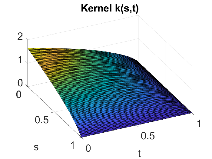

The right picture shows that the partial derivative has a pole at the right boundary with of the unit square. This pole implies that . On the other hand, is smooth elsewhere and allows for further partial differentiation with a second partial derivative
| (32) |
which has also a pole at . We note that the order of the pole there is growing by one for every higher partial differentiation step with respect to .
Based on (32) one can derive, in light of formula (26) from Lemma 3, that
with and . Notice, that , which prevents the application of Lemma 3, even in the case . Thus, Lemma 3 is not applicable, and we may not make inference on the decay rates of the singular values by means of considering kernel smoothness.
Remark 7.
We have not found assertions in the literature, which handle the situation of such poles in light of decay rates of singular values.
In summary, the smoothness of the kernel from (28) is strongly limited. In particular we have . This makes an exponential decay rate of the singular values appear rather unlikely. However, at present we have no analytical approach to check this in more detail.
5. Bounding the singular values of the composite operator
Our aim of this section is to improve the upper bound in (25) for the singular values of the composite operator
| (33) |
We emphasize that this composition constitutes a Hilbert-Schmidt operator, since its component is Hilbert-Schmidt, and our argument will be based on bounding the Hilbert-Schmidt norm
The main result will be the following.
Theorem 3.
For its proof we make the following preliminary considerations. We recall the definition of the shifted Legendre polynomials from (19), as well as , being the orthogonal projection onto the -dimensional subspace of the polynomials up to degree .
For the further estimates the next result is important. Here, we denote by the singular system of the compact operator .
Proposition 3.
Let denote the projections onto of the Legendre polynomials up to degree , and let be the singular projection onto of the first eigenelements of . Then we have for that
Proof.
We shall use the additivity of the singular values, i.e., it holds true that
In particular we see that
because vanishes by definition of . Consequently we can bound
with equality for being the singular projections . ∎
Finally we mention the following technical result, which is well-known. For the sake of completeness we add a brief proof.
Lemma 4.
Let be non-increasing, and let . Suppose that there is a constant such that for . Then there is a constant such that for
Proof.
We can estimate as
which gives and proves the lemma. ∎
Let us introduce the normalized functions
Lemma 5.
For each we have that
Proof.
Proof of Theorem 3.
Since the system of shifted Legendre polynomials is an orthogonal basis in , we have by virtue of [19, Thm. 15.5.5] that
| (35) |
and we shall bound by using Lemma 5 that
| (36) | ||||
| (37) |
The norm square within the above sum is less than or equal to one, such we arrive at
The sum on the right is known to be minus one half of the second derivative of the digamma function, see [1, (6.4.10)]. Thus we have
| (38) |
Moreover, from the series expansion of the digamma function, see [1, (6.4.13)], we see that , which implies
| (39) |
for sufficiently large . Finally, applying Proposition 3 and Lemma 4 (with and ) we see that for some constant . This completes the proof. ∎
6. Discussion
We extend the previous discussions in a few aspects. As it is seen from Corollary 2 and Theorem 3 there is a gap for the composition between the obtained decay rate of the order of the singular values and the available lower bound of the order as . We shall dwell on this further, and we highlight the main points that are responsible for the lower and upper bounds, respectively.
The overall results are entirely based on considering the Legendre polynomials as means for approximation. Clearly, these play a prominent role in our handling of compositions that contain the operator . In particular, the normalized polynomials constitute an orthonormal basis in , and the upper bounds from Lemma 2 show that these are suited for approximation. However, as a consequence of using the Legendre polynomials we arrive at the -sections of the Hilbert matrix , see Lemma 1. As emphasized in the proof of Theorem 2, the condition numbers of the Hilbert matrix are of the order , and this in turn yields the lower bound, after applying Theorem 1. Despite of the fact that this general result may not be sharp for non-commuting operators in the composition, we may argue that using -sections is not a good advice for obtaining sharp lower bounds. So, it may well be that the lower bounds could be improved by using other orthonormal bases than the Legendre polynomials.
The obtained upper bound is based on the approximation of by Legendre polynomials in the Hilbert-Schmidt norm, and we refer to the inequality (39). There are indications in our analysis, for example in the context of (37), that this bound cannot be improved, but what when using other bases?
Another aspect may be interesting. While we established an improved rate for the composition , this is not possible for the composition , see the discussion in Section 1. In the light of the spectral theorem, and we omit details, the operator is orthogonally equivalent to a multiplication operator mapping in with a multiplier function and possessing zero as accumulation point, and isometries and , for which we have . This implies that
Clearly we have that , which looks very similar to the problem of the composition , where but with the intermediate isometry . Therefore, we may search for isometries such that we arrive at
Clearly, this holds true for the identity, and this does not hold true for from above connected with the Hilbert matrix. Because isometries turn orthonormal bases onto each other, we are again faced with the problem, which approximating orthonormal basis is best suited as means of approximation in the composition . Thus, the results presented here are only a first step for better understanding the problem of approximating a composition of a compact mapping followed by a non-compact one.
Acknowledgment
The authors express their deep gratitude to Daniel Gerth (TU Chemnitz, Germany) for fruitful discussions and that he kindly provided Figure 1. We also appreciate thanks to Robert Plato (Univ. of Siegen, Germany) for his hint on studying the Fredholm integral operator kernel of in , which gives additional motivation. Bernd Hofmann is supported by the German Science Foundation (DFG) under the grant HO 1454/13-1 (Project No. 453804957).
Appendix A Proof of Proposition 1
To prove the series representation (28) for the kernel of , we start with
Integration part parts yields
| (40) |
Taking into account the well-known structure of the adjoint operator of (see, e.g., [7, Proposition 3]), we can further write
Applying the operator from the left, for which the analytical structure is also well-known, and we find again using integration by parts the formulas
We can rewrite this as
which shows the representation (28), and this completes the proof.
References
- [1] M. Abramowitz and I. A. Stegun, Handbook of Mathematical Functions with Formulas, Graphs, and Mathematical Tables, National Bureau of Standards Applied Mathematics Series, No. 55 U.S. Government Printing Office, Washington, D.C., 1964.
- [2] D. D. Ang, R. Gorenflo, V. K. Le, and D. D. Trong, Moment Theory and Some Inverse Problems in Potential Theory and Heat Condution, Springer-Verlag, Berlin-Heidelberg, 2002.
- [3] B. Beckermann, The condition number of real Vandermonde, Krylov and positive definite Hankel matrices, Numer. Math., 85(4):553–577, 2000.
- [4] R. Bot,̧ B. Hofmann and P. Mathé, Regularizability of ill-posed problems and the modulus of continuity, Z. Anal. Anwend. 32(3):299-312, 2013.
- [5] S.-H. Chang, A generalization of a theorem of Hille and Tamarkin with applications, Proc. London Math. Soc. (3)2:22–29, 1952.
- [6] M. Freitag and B. Hofmann, Analytical and numerical studies on the influence of multiplication operators for the ill-posedness of inverse problems, J. Inverse Ill-Posed Probl., 13(2):123–148, 2005.
- [7] D. Gerth, B. Hofmann, C. Hofmann and S. Kindermann, The Hausdorff moment problem in the light of ill-posedness of type I, Eurasian Journal of Mathematical and Computer Applications, 9(2):57–87, 2021.
- [8] F. Hausdorff, Momentprobleme für ein endliches Intervall (German), Math. Z., 16(1):220–248, 1923.
- [9] B. Hofmann and S. Kindermann, On the degree of ill-posedness for linear problems with non-compact operators, Methods Appl. Anal., 17(4):445–461, 2010.
- [10] B. Hofmann, P. Mathé and M. Schieck, Modulus of continuity for conditionally stable ill-posed problems in Hilbert space, J. Inverse Ill-Posed Probl., 16(6):567–585, 2008.
- [11] B. Hofmann and L. von Wolfersdorf, Some results and a conjecture on the degree of ill-posedness for integration operators with weights, Inverse Problems, 21(2):427–433, 2005.
- [12] B. Hofmann and L. von Wolfersdorf, A new result on the singular value asymptotics of integration oprators with weights, J. Integral Equations Appl., 21(2):281–295, 2009.
- [13] G. Inglese, Recent results in the study of the moment problem, In: Theory and Practice of Geophysical Data Inversion, Proc. of the 8th Int. Math. Geophysics Seminar on Model Optimization in Exploration Geophysics 1990, Vieweg, Braunschweig-Wiesbaden, 1992, pp. 73–84.
- [14] H. König, Eigenvalue distribution of compact operators, Birkhäuser Verlag, Basel, 1986.
- [15] S. Lu, V. Naumova and S. V. Pereverzev, Legendre polynomials as a recommended basis for numerical differentiation in the presence of stochastic white noise, J. Inverse Ill-Posed Probl., 21(2):193–216, 2013.
- [16] M. Z. Nashed, A new approach to classification and regularization of ill-posed operator equations, In: Inverse and Ill-posed Problems Sankt Wolfgang, 1986, volume 4 of Notes Rep. Math. Sci. Engrg. (Eds.: H. W. Engl and C. W. Groetsch), Academic Press, Boston, 1987, pp. 53–75.
- [17] A. Pietsch, -numbers of operators in Banach spaces, Studia Math., 51:201–223, 1974.
- [18] A. Pietsch, Eigenvalues and -numbers, Cambridge Studies in Advanced Mathematics, Cambridge University Press, Cambridge, 1987.
- [19] A. Pietsch, Operator Ideals, Mathematische Monographien [Mathematical Monographs] Vol. 16, Dt. Verlag der Wissenschaften, Berlin, 1978.
- [20] J. B. Reade, Eigenvalues of positive definite kernels, SIAM J. Math. Anal., 14(1):152–157, 1983.
- [21] J. B. Reade, Eigenvalues of Lipschitz kernels, Math. Proc. Cambridge Philos. Soc., 93(1):135–140, 1983.
- [22] G. Talenti, Recovering a function from a finite number of moments, Inverse Problems, 3(3):501–517, 1987.
- [23] J. Todd, The condition number of the finite segment of the Hilbert matrix, Nat. Bur. of Standards Appl. Math. Series, 39:109–116, 1954.
- [24] Vu Kim Tuan and R. Gorenflo, Asymptotics of singular values of fractional integral operators, Inverse Problems, 10(4):949–955, 1994.
- [25] H. Wang, S. Xiang, On the convergence rates of Legendre approximation, Math. Comput., 81:861–877, 2012.
- [26] H. S. Wilf, Finite Sections of Some Classical Inequalities, Springer-Verlag, New York-Berlin, 1970.
- [27] Z. Zhao, A truncated Legendre spectral method for solving numerical differentiation, Int. J. Comput. Math., 87(14):3209-3217, 2010.