Quantum Kinetic Theory of Plasmas
Abstract
As is well-known, for plasmas of high density and modest temperature, the classical kinetic theory needs to be extended. Such extensions can be based on the Schrödinger Hamiltonian, applying a Wigner transform of the density matrix, in which case the Vlasov equation is replaced by the celebrated Wigner-Moyal equation. Extending the treatment to more complicated models, we investigate aspects such as spin dynamics (based on the Pauli Hamiltonian), exchange effects (using the Hartree-Fock approximation), Landau quantization, and quantum relativistic theory. In the relativistic theory we first study cases where the field strength is well beyond Schwingers critical field. Both weakly relativistic theory (gamma factors close to unity) and strongly relativistic theory are investigated, using assumptions that allow for a separation of electron and positron states. Finally, we study the Dirac-Heisenberg-Wigner (DHW) formalism, which is a fully quantum relativistic theory, allowing for field strengths of the order of the Schwinger critical field or even larger. As a result, the quantum kinetic theory is extended to cover phenomena such as Zitterbewegung and electron-positron pair creation. While the focus of this review is on the quantum kinetic models, we illustrate the theories with various applications throughout the manuscript.
Keywords:
Quantum kinetic theory, Density matrix, Wigner transform, Exchange effects, Dirac-Heisenberg-Wigner formalismI Introduction
Historically, the vast majority of plasma physics has been limited to classical (non-quantum) phenomena. With important applications, such as magnetically confined fusion plasmas and space plasmas, where the density is modest and the temperature is high, the focus of plasma physics on classical models has been natural. However, in recent times, much work (see e.g. Refs. Manfredi-2019; Shukla-Eliasson-2011; Melrose-2020; Shukla-Eliasson-2011-2; Vladimirov-review, and references therein) has been devoted to the regime of high density and a low or modest temperature, allowing for quantum mechanical phenomena to influence the dynamics. We will come back to which concrete systems that can be of interest in such a context.
Out of the possible quantum effects, maybe the most basic one is particle dispersion (see e.g. Haas-book-chap2; ManfrediWigner-Numerics; Haas-Shukla 2008; Haas-mfl-2008). This spread out in the wave function is captured already in the Schrödinger equation, but arguably this is one of the most important quantum mechanical mechanisms. Another basic, and important, phenomenon is the degeneracy effect Manfredi-2019; Shukla-Eliasson-2011; Melrose-2020; Shukla-Eliasson-2011-2; Vladimirov-review; Vladimirov-surf1; Vladimirov-surf2, entering when the density becomes high enough to make the Fermi temperature significant in relation to the thermodynamic temperature. A related phenomena, also dependent on the antisymmetry of the manybody wavefunction of electrons, but considerably more complicated to model mathematically, is the exchange interaction Manfredi-exchange; Haas-exchange; Andreev-exchange; Egen-2013-exchange; Egen-2015-exchange; Egen-2015-second-exchange; Egen-2019-exchange, whose importance probably has been undervalued in the recent plasma research literature. Upgrading from the Schrödinger Hamiltonian to the Pauli-Hamiltonian, the spin dynamics enter the picture Manfredi-spin1; Brodin2008; Zamanian 2010; Andreev-spin1; Andreev-spin2; Andreev-spin3; Andreev-spin4, with physics such as the magnetic dipole force, spin precession, and (spin) magnetization currents. Extending the models to cover the weakly relativistic regime Asenjo-2012; Hurst-2017; Ekman-2021, spin-orbit interaction, Thomas precession and a spin-dependent polarization current are new features of the theory. Finally, in the regime of strong fields strongfield1; strongfield2 and fully relativistic theory BB-1991, phenomena such as strong Landau quantization landau-quant and electron-positron pair creation BB-1991; Al-Naseri-2021; Gies2; Sheng; Kohlfurst-2020; titopar come into play.
Before proceeding to the the more theoretical aspects, we should get an idea what concrete systems that are of interest. One such answer is explored in some detail in the recent review by Manfredi et al. Manfredi-2019, where metallic nano-objects are in focus. As described in that work, the properties of metallic particles ranging in size from a few to several hundred nanometer can be well modeled with quantum kinetic theory. Importantly, the nano-particles are of interest for applications in nano-photonics and other technological applications.
Furthermore, by identifying the quantum regime in a density temperature diagram, as done, e.g., by Refs. Bonitz-book; Asenjo-2012 a reasonably complete picture of quantum plasmas can be presented. Besides the solid state regime, that might be of most technological interest (including applications to e.g., spintronics Spintronics, plasmonics Plasmonics, nanotubes Nanotubes, quantum wells Quantum-wells and quantum dots Quantum-dots), quantum plasmas can be found in rather diverse contexts, including dense astrophysical objects astro1; astro2 (white dwarf stars neutron stars), warm dense matter, laboratory plasmas Glenzer, and plasmas in the early universe early universe. However, assuming that the plasma need to occupy a specific spot in a temperature-density diagram, for quantum effects to be significant, sometimes lead to the wrong conclusion. For example, strong laser fields may potentially induce quantum phenomena such as spin polarization, as explored in Refs. SP-1; SP-2; SP-3. Moreover, in an astrophysical context, strong magnetic fields from pulsars and/or magnetars magnetar may lead to very pronounced Landau quantization. Finally, as we will discuss in section VI, a sufficiently strong electrostatic field lead to Schwinger pair production of electrons and positrons BB-1991; Al-Naseri-2021; Gies2; Sheng; Kohlfurst-2020. Thus, when intense electromagnetic fields are involved, there are several ways quantum phenomena can enter the picture, even when the parameters of density and temperature correspond to the classical regime.
The paper is organized as follows: In section II we study foundations of quantum kinetic theory, in particular the density matrix, the von Neumann equation, and the Wigner transform Wigner32. To focus on the fundamentals, for much of the section we avoid the complications of spin and electromagnetic fields, and base the treatment on the simplest form of the Schrödinger equation. The theory is illustrated with examples from linear theory. In section III, the treatment is extended to cover many particle physics (in the quantum mechanical sense). In particular, the quantum mechanical version of the BBGKY-hierarchy is used to study exchange interaction, with a particular focus on electrostatic linearized theory. Exchange corrected dispersion relations are computed, for Langmuir waves and ion-acoustic waves, in the degenerate and non-degenerate regime. In section IV, we allow for electromagnetic fields and spin dynamics. For that purpose, the Schrödinger Hamiltonian is replaced with the Pauli Hamiltonian. Two equivalent but different versions of quantum kinetic theory is presented. The linear theory of the model is solved in the long-scale limit for the case of a homogeneous magnetized plasma, generalizing previous results to include an anisotropic background distribution. Next, in section V, a multitude of different problems are discussed that is not covered by the previous theories. This includes quantum kinetic conversation laws, relativistic Landau quantization, and aspects of nonlinear spin dynamics, focusing on the ponderomotive force. In section VI, we study the fully quantum relativistic case, using the Dirac-Heisenberg-Wigner (DHW) formalism, originally derived by Ref. BB-1991. The equations are used to study electrostatic fields, and some deviation from simpler theories are pointed out. Moreover, we show how to relate the DHW-formalism to limiting cases studied in the previous sections. Finally, the paper ends with concluding remarks in section VII.
II The Gauge-Invariant Wigner Theory
The aim of this section is to give a brief introduction to how the Wigner functions can be used to describe quantum effects in plasmas. In order to this, we start with a review of the density matrix and some of its properties. After that, we go on to define the Wigner transformation, which is a transformation that brings the evolution equation in a form similar to classical kinetic theory. We comment on the interpretation of the Wigner function and some of the key properties. Finally, we consider a system in an electromagnetic-field and give a description of the gauge-invariant Wigner function and the corresponding evolution equation.
II.1 The Density Matrix
In order to describe an -particle system, where the initial state is known we can use a many-particle wave function . Here is the position for the :th particle and , is the probability of simultaneously measuring the particles at respective positions in the volume around . Assuming that the particles have mass and are moving in a potential , the evolution follows the Schrödinger equation
| (1) |
supplemented by the initial state of the system
| (2) |
The exact state of a multi-particle system cannot be known in general, instead the best we can hope for is the knowledge of a statistical distribution of states. In order to handle this situation in it is then necessary to use the so called density matrix. It is defined as
| (3) |
where is the probability of finding the system in state , and the sum is over all states that the system can be in. From normalisation we require that
| (4) |
which can be interpreted that the total probability of finding the system in one of the states is unity. E.g., in the case where the system is in thermal equilibrium with temperature , the density matrix is
| (5) |
where
| (6) |
is the partition function, and the sum is over all eigenstates to the Hamiltonian, .
From the definition above together with the Schrödinger equation (and its complex conjugate), it is we can derive the evolution equation for the density matrix
| (7) |
This is called the von Neumann equation, or alternatively, the quantum Liouville equation (see e.g., Ref. Bonitz-book). The density matrix describes the system completely, and we can use it to calculate, e.g., the probability of finding the particles at respective positions as the diagonal elements
| (8) |
One thing to note about the density matrix is that it changes under a gauge-transformation. E.g., in case of a single particle interacting with an electromagnetic field described by the potentials , , a gauge transformation
| (9) | ||||
| (10) |
the density matrix transforms as
| (11) |
where is the charge of the particle, see e.g., Sakurai-book. In the -particle case, the density matrix obtains a phase-factor for each , and a factor for each .
The density matrix encodes all the information about the system. However, the evolution equation (7) involves a huge number of variables, six for each particle, so it is not directly applicable when considering plasmas. In Appendix A, we derive the mean-field approximation, which is a common approximation used when modelling plasmas. We here state the most important conclusions. In the mean-field approximation density matrix only depends on two variables
| (12) |
where the diagonal elements yields the density of particles at a given position in space
| (13) |
with the normalisation
| (14) |
where is the total number of particles. The mean-field Hamiltonian formally looks like it is describing a one-particle system, but is modified in that the fields are the self-consistent fields created by all the particles. For example, for an electrostatic plasma we have
| (15) |
where is the self-consistent field, which is relate to the particle density via Poisson’s equation
| (16) |
Here we have added a neutralising and homogeneous charge density . The mean-field approximation is usually applicable in cases where particle correlations can be neglected. E.g., in cases where particle-particle collisions can be neglected. By including further terms in the BBGKY-hierarchy it is possible to include particle collisions, see e.g., Ref. Bonitz-book In the discussion above we have also neglected any reference to the particle statistics. Since we are dealing with fermions one should really take into account the anti-symmetry of the wave function. In Section III we generalise the mean-field approximation to account for this. The resulting approximation is usually called the Hartree-Fock approximation.
II.2 The Wigner Transformation
A key tool when deriving quantum kinetic equations from the Schrödinger or Pauli Hamiltonian is the Wigner transform, introduced by Eugene Wigner in his famous paper from 1932 Wigner32. Using this transform on the density matrix, a kinetic evolution generalizing the classical Vlasov equation can be derived. This connection with classical theory is helpful for guiding the physical intuition, and the transformed quantities are typically more attractive for practical calculations. Wigner’s original approach has been further developed by others, in particular José Enrique Moyal Moyal-1949, and the Wigner equation is sometimes also referred to as the Wigner-Moyal equation.
The Wigner transform of the density matrix is defined by
| (17) |
We can see that e.g.,
| (18) |
gives the local density of particles, and similarly
| (19) |
is the momentum distribution of the particles. However, in contrast to the Vlasov distribution, the Wigner distribution can be negative in certain regions. This is attributed to the Pauli exclusion principle, and we should hence be careful in interpreting the Wigner function as a classical phase-space distribution. Irrespective of that, the Wigner function can still be used to calculate macroscopic properties of the system, such as, e.g., the charge and current densities.
If the system is described by the Hamiltonian, (15), we can derive the evolution equation for using the Schrödinger equation as follows: The evolution equation for the density matrix is given by
| (20) |
Using the variable change
| (21) |
the equation is cast into
| (22) |
We now want to take the Fourier transformation of this and re-identify the Wigner function in each term. In order to do this, we can use the following trick
| (23) |
where is defined by its Taylor expansion. Here the arrow over indicates that the operator should act to the left on the exponential function only. For the term containing we make a partial integration. Doing this we finally get the equation
| (24) |
In the mean-field approximation, the equation above describes a system of particles interacting via the electric potential created by all the particles via
| (25) |
where we have assumed that there is a homogeneous, neutralizing background of particles with charge density (note, for electrons with our conventions). These two equations together with the appropriate initial conditions yields the dynamics of the system.
The Wigner distribution function, can be used to calculate any expectation value in a similar way to how this is done in classical kinetic theory. For example we have
| (26) |
For a general operator , depending on both the position and momentum variables, we must first put all the position and momentum operators in completely symmetric form using the commutation relations, and then replace all operators with the corresponding phase-space variables. For example, to calculate the expectation value of the operator we first write
| (27) |
So the phase-space function corresponding to is . Note, that this particular operator is not physical since it is not hermitian, we only chose it to illustrate the procedure. This correspondence between operators and phase-space functions is called Weyl ordering, see e.g., qmps.
As an example, consider linear waves where the distribution function can be written
| (28) |
where is a spatially homogeneous equilibrium, e.g., a Maxwell-Boltzmann distribution. Similarly we write the potential as
| (29) |
Linearising the evolution equations above and solving for we get the dispersion relation
| (30) |
where the last equation is obtained by a change of variables. In the limit , this reduces to the classical Vlasov dispersion relation. This dispersion relation has been investigated in detail in Ref. eliason-shukla-09. There it is shown that for a fully degenerate background distribution (), the wave particle damping disappears in the Vlasov limit, since the phase-velocity always exceeds the Fermi velocity. Furthermore, the critical wave number , at which the Landau damping sets in, was computed.
Returning to the general case, Eq. (24), it is straightforward to show that this equation reduces to the classical Vlasov equation for long macroscopic scale lengths. In particular, if the potential varies on a scale length , i.e. , and the characteristic velocity of the system is , , then in the limit
| (31) |
we may keep the first non-vanishing terms in a Taylor expansion of the potential in Eq. (24). We then get
| (32) |
i.e., the Vlasov equation, where . By keeping further terms in the expansion we may use this method to derive quantum corrections to an arbitrary order, see, e.g., Ref. Waterbag.
II.3 The Gauge-Invariant Wigner Function
The Hamiltonian describing a charged particle of mass and charge ( for electrons) interacting with a magnetic field is given by
| (33) |
where and are the (mean-field) electromagnetic potentials. Note that, here is the canonical momentum operator, and it is related to the velocity via the vector potential in the usual way. If the state of the particle is described by the density operator , the evolution of the system is given by the von Neumann equation (159). As we have seen, above, the equation can also be used to describe a system of particles interacting with the mean-field created by all the other particles. In that case, the density operator should be interpreted as the reduced density operator. This is the point of view we will take here.
Under a gauge transformation the density matrix changes according to Eq. (11). Due to this, the Wigner function , defined in Eq. (17) will not be gauge-invariant. Furthermore, the momentum variable, will be related to the velocity in a gauge-dependent way. In order to get something that is more attractive to work with, we will use a modified version of the Wigner transformation, first constructed by Stratonovich strato. The definition is
| (34) |
An important aspect of this transformation, is that the momentum variable , is the kinetic momentum related to the velocity via . This can be seen by calculating the momentum density
| (35) |
where denotes the anti-commutator. The right hand side can be identified as the (kinetic) momentum density. From the evolution equation for the density matrix we can derive the evolution equation in the gauge invariant case in a similar fashion as in the previous sub-section. The result is serimaa
| (36) |
where
We note that, since the equation is completely expressed in terms of the electric and magnetic field, it is manifestly gauge-invariant. Also, since the momentum variable involved is the kinetic momentum, we may make the trivial variable change and express the Wigner function as . In the classical limit, i.e. when Eq. (31) applies, this reduces to the Vlasov equation. By Taylor-expanding the functions , and , it is possible to obtain approximations to arbitrary order in .
The models we have explored in this section are of importance in their own right, and have been used, for example, to consider quantum dispersive effects, see e.g., Refs. Shukla-Eliasson-2011; Vladimirov-review and references therein. However, in what follows, we will continue with more elaborate models including additional physical phenomena, such as exchange effects, spin, and relativistic effects.
III Exchange effects
Exchange interaction in plasmas follows from electrons being fermions, with a totally anti-symmetric wavefunction. To include exchange effects it is not enough to just use the Slater determinants to construct the many-body wave-functions from single-particle wave-functions (although this is a necessary first step). Nor will it suffice to simply infer Fermi-Dirac statistics of the background plasma. Instead one must go go beyond the simplest mean-field description. Covering exchange effects is usually referred to as the Hartee-Fock approximation Hartree-Fock, in contrast to the Hartree approximation, where exchange effects are ignored.
The relative importance of exchange effects in plasmas is proportional to the parameter Manfredi-exchange; Haas-exchange; Egen-2013-exchange; Egen-2015-exchange; Egen-2015-second-exchange; Egen-2019-exchange, where the characteristic kinetic energy is given by for a degenerate plasma (with ) and by for the non-degenerate case (with ). The above suggests that exchange effects are as important as the more basic particle dispersive effects, described by the Wigner-Moyal equation of the previous section. If so, the common approach of including particle dispersive effects through the Wigner equation, but simultaneously neglecting exchange effects would be highly questionable. Fortunately, while the relative importance scales with temperature and density as given by the -parameter, the overall importance is also proportional to another dimensionless constant that often is much smaller than unity Egen-2019-exchange. Hence the use of the Wigner equation from the preceding section, neglecting exchange effects, can still be a good approximation. What complicates the picture, is that the importance of exchange effects it not just dependent on the background plasma parameters (temperature and density), but also of the specific problem under study. Below we will illustrate this by considering simple examples of high-frequency Langmuir waves, and low-frequency ion-acoustic waves.
III.1 General electrostatic theory
Since the theory becomes more complicated for the electromagnetic case, we here present a general quantum kinetic approach to exchange effects in the electrostatic limit. The full electromagnetic case will be discussed briefly in the end of Section III.
Our treatment will follow Ref. Egen-2013-exchange, but leaving out some of the technical details. We here consider a completely ionized electron-ion plasma with the particles interacting through a mean-field scalar potential. Quantum effects for the ions will be completely neglected as will effects due to the self-energy and particle correlations Bonitz-book. The state of the -electrons is described by the density operator (see for example Ref. Bonitz-book), and the dynamics is given by the von Neumann equation with the Hamiltonian
| (37) |
The last term accounts for the interaction with the electric potential created by the ions. In Appendix A we derive the mean-field approximation, in the case where we can neglect exchange effects. Here we generalize (163) to take into account the anti-symmetry of the wave function for the electrons. We introduce the reduced density operators according to
| (38) |
where denotes the trace over particles to (i.e. integrating over the position degree of freedom and summing over the spins), and is the anti-symmetrization operator that takes an -particle state and makes it completely anti-symmetric db79. We will only need to know that where interchanges particle 1 and 2, i.e. (see, e.g., Ref. Bonitz-book for further details). The evolution for the one-particle density operator is given by
| (39) |
where and and is the two-particle density operator. The effects of two-particle correlations can be separated out of the two-particle density operator by writing it in the form
| (40) |
see e.g., Ref. wang85. We are interested in the collisionless limit where a mean-field approximation will suffice. This approximation is obtained by neglecting the correlation . Utilizing this in Eq. (39) we obtain
| (41) |
where , is the Hartree-Fock potential operator. This is a closed system for the one-particle density operator.
To obtain a connection to the classical kinetic theory we use the Wigner representation Wigner32 of this equation. Using the complete set of states , where is the position and is the spin along the axis of quantization, this representation is obtained as
| (42) |
where is the density matrix. This is a slight generalisation of Eq. (17), where we trivially include the spin-variables. Note, however, that the resulting Wigner function depends on the two spin-variables and is hence a 2-by-2 matrix. Writing Eq. (41) first in the position representation and Wigner transforming the result (using e.g., the method outlined in Section II.2) we obtain,
| (43) |
where
| (44) |
is the total (mean-field and the ionic field) potential and
| (45) |
is the Coulomb potential. The left hand side of Eq. (III.1) represents the electrostatic limit of the Wigner-Moyal equation, but keeping the spin-dependence (as encoded in ) while the right hand side is the correction due to exchange effects. This term is nonlocal in phase-space and nonlinear in the distribution function.
Two steps of our general treatment remain, taking the long-scale limit and averaging over the spin states . The first step is straightforward, just expanding the equations in . The second step takes a little more work, but can be done with the help of the spin transform. The spin transform will be discussed in detail in the next section (Section IV), and the details regarding the procedure for our specific case can be found in Ref. Egen-2013-exchange. Thus we will omit these details here, and proceed directly to the end result, the spin averaged evolution equation (assuming all spin directions equally probable) in the long scale limit (). The evolution equation then reads
| (46) |
where and analogously for and an arrow above an operator indicates in which direction it acts. We have also used the summation convention so that a sum over indices occurring twice in a term is understood.
III.2 High-frequency Langmuir waves
Eq. (46) is derived using a perturbative approach where exchange effects are considered to be small. Thus there is little reason trying to solve Poisson’s equation together with (46) exactly. Instead we first solve Eq. (46) dropping the right hand side altogether (i.e. we solve the Vlasov equation), and then substitute these solutions into the right hand side, in order to evaluate the exchange correction to first order. Even this simplified treatment might be rather difficult, unless the zero order Vlasov solution is fairly simple. In order to focus on a case that can be treated analytically to a large degree, we now consider the case of linear Langmuir waves in a homogeneous plasma. The general procedure is as follows:
- 1.
Pick a background distribution function (e.g. a Maxell-Boltzmann or a Fermi-Dirac distribution), linearize the left hand side Vlasov equation, make a plane wave ansatz, and compute the perturbed distribution function.
- 2.
Linearize the right hand side exchange term (keep terms where one factor is the linear perturbation, and the other is the background), substitute the distribution functions from the previous step and compute the integrals, and find the exchange correction to the perturbed distribution function.
- 3.
Make a final momentum integration to find the exchange contribution to the charge density, and use this in Poisson’s equation to find the exchange correction to the susceptibility.
Treating the ions as immobile, considering a Maxwell-Boltzmann background distribution for the electrons, and performing the steps outlined above, Ref. Egen-2015-exchange was able to derive the following result:
| (47) |
Here is the classical electron susceptibility, given by , and is the exchange correction to the susceptibility, given by
| (48) |
where the velocity integrations (normalized against the thermal velocity) covers all of velocity space. In general, the last integrals to find must be solved numerically. However, the case of most interest is when , such that the Landau damping is weak, in which case we can expand the integrals in powers of . To leading order in , neglecting the pole contribution associated with Landau damping altogether, Eq. (47) reduces to
| (49) |
After correcting a slight numerical error in equation (49) of Ref. Roos we note that the result there is exactly a factor two larger than our result above. The difference is due to that Ref. Roos does not take into the spin part of the wavefunction. We note that it is the full many-body wavefunction that should be anti-symmetric with respect to particle interchange, not just the spatial part. Ignoring this over-estimates the exchange correction by a factor of two.
While the scaling with temperature and density is the same as for many other quantum phenomena (proportional to ) , we note that the overall factor also contains the small dimensionless number which appears for geometrical reasons. Due to this small number, it makes sense to ignore exchange effects at the same time as other quantum effects are kept. However, as we will see below, there is no general principle guaranteeing the relative smallness of exchange effects. Thus, whether or not exchange effects can be ignored for other specific problems, as compared to particle dispersive effects, is an open question in general. The next sub-section will deal with ion-acoustic waves. However, before ending this sub-section, we note that the case of degenerate electrons require different integrals to be solved. We omit this case here, but point out that the exchange contribution to the Langmuir wave dispersion relation with a fully degenerate Fermi-Dirac background distribution can be found in Ref Egen-2015-second-exchange.
III.3 Low-frequency ion-acoustic waves
The general procedure numbered 1-3 of the previous sub-section still applies for ion-acoustic waves. However, the concrete integrals that need to be solved depend on whether the electrons are degenerate or non-degenerate (assuming we limit ourselves to a thermodynamic background distribution). Also, the integration will be simplified in the quasi-neutral regime, that applies for frequencies . An additional thing to consider is the Landau damping, that often can be neglected for Langmuir waves, but generally tends to be significant for ion-acoustic waves. Thus we must use the Landau contours when evaluating the integrals, and keep track of both the real and imaginary parts. The case of cold classical ions and a Maxwell Boltzmann distribution for electrons was considered by Ref. Egen-2013-exchange, and the dispersion relation in the quasi-neutral limit was found to be
| (50) |
where is the classical ion-acoustic velocity and we have introduced the classical electron Landau damping, , in the cold ion limit boyd. The coefficients of the real and imaginary quantum terms ( and , respectively) are only approximate, as the final step involves a numerical integration. An important result from this calculation is that the exchange corrections now is proportional to a factor of the order unity times the quantum parameter , in contrast to the previous case of Langmuir waves. As a consequence, when studying short scale dynamics, it is not a good approximation to keep the particle dispersive terms through the Wigner-Moyal equation, and simultaneously drop the exchange contribution.
Next, we turn our attention to the same case as above, but with degenerate electrons. In the quasi-neutral limit, the dispersion relation can then be computed as (see, e.g. Ref. Egen-2015-second-exchange for details]
| (51) |
where . Apparently, the relative magnitude of the exchange terms are even larger than for the non-degenerate case, and, accordingly, independently of the background distribution, the omission of exchange terms in the quantum regime cannot be justified for ion-acoustic waves.
III.4 Exchange effects - final discussion
As illustrated above, due to the non-trivial momentum integrals, a first principal kinetic treatment of exchange effects is complicated. Going beyond the simplest cases, like the ones studied above, would require a major numerical effort. Even so, only perturbative treatments where exchange effects are small would be possible. However, the topic is an important one, as exchange effects are not generally small compared to other quantum effects. A tentative conclusion, suggested by the above findings, would be that the exchange contribution might be limited (to the extent that it could be negligible) for high-frequency phenomena, but not for low-frequency phenomena. However, more studies need to be done to put such a conclusion on a firm ground.
An important generalization of the above treatment, is to cover also electromagnetic phenomena. Some key steps toward that goal was taken in Ref. Egen-2015-exchange, although no concrete examples were worked out. An important issue to address in this case is the gauge invariance, as the exchange integrals tend to be dependent on the electromagnetic potentials, rather than the electromagnetic fields.
In light of the challenging nature of the kinetic exchange contribution, it would be valuable to have less complex models, allowing for computational progress also beyond the perturbative regime. A quantum hydrodynamical model fulfilling this criterion has been put forward by Ref. Manfredi-exchange. In addition to exchange effects, this model also covers the effect of electron correlations. Importantly, the hydrodynamical model is easy to use for practical calculation, as the exchange and correlation terms does not add much extra difficulty compared to pressure and particle dispersive terms. However, a drawback is that the model is based on time-independent density functional theory, and hence the applicability to dynamical phenomena is uncertain at best. A comparison of the hydrodynamical and kinetic models, to some extent covering regimes not presented above, has been made in Ref. Egen-2019-exchange, and the numerical comparisons are shown in Figs 1 and 2, borrowed with permission from the original source. The overall conclusion is that there is a reasonable agreement between the hydrodynamic and the kinetic models in the long wavelength high-frequency regime, but otherwise the hydrodynamical model tend to largely underestimate the importance of exchange effects.
IV The Pauli Hamiltonian and Spin dynamics
Next we will generalize the treatment based on the Scrödinger equation to include the spin dynamics. In principle the formalism is similar to that of section II. In particular the higher order terms in the BBGKY-hierarchy BBGKY are dropped, and thus the evolution equation will be derived from the single particle density matrix, using the von Neumann equation, followed by a Wigner-transform. Nevertheless, there is an important difference compared to the previous case, as the density matrix now depend on the spin state. As a result, the single component in the Scrödinger case is replaced by a two by two matrix, where the different components represent different spin states. The changes needed to obtain the kinetic evolution equation are outlined in subsection A, and two different but equivalent systems are presented. Then, in subsection B, we use the model to derive the linear conductivity tensor in a magnetized plasma, generalizing previous results to cover the case of an an-isotropic background distribution.
IV.1 Derivation of evolution equations
Including the spin dynamics, in the lowest (non-relativisitic) approximation, we replace the Schrödinger Hamiltonian of Section II with the Pauli Hamiltonian
| (52) |
where here denotes a vector with the Pauli matrices as components. Following Ref. Zamanian 2010, we are able to construct a gauge invariant scalar kinetic theory using a density matrix description for a spin-1/2 particle.
The basis states are , where is a state with position and is the state with spin-up or spin-down . As a starting point for the derivation, we use the spinor state which fulfill the dynamical equation , with the Hamiltonian (52). The density matrix is now given by
| (53) |
where, as before, is the probability to have a state , but we have the additional dependence on spin state. Similarly as before, the von Neumann equation applies, i.e. the evolution equation for the density matrix is
| (54) |
Once the density matrix has been defined, we can define the Wigner-Stratonovich transform strato as
| (55) |
where the phase
| (56) |
is used to ensure gauge invariance of the resulting distribution function. This is the same transformation as in Eq. (34) with the modification that it must to be taken separately for each component of the 2-by-2 density matrix.
In principle, Eq. (54) together with Eq. (55) gives us a kinetic evolution equation, and we could be content with this. However, the individual components of have no clear physical interpretation, and it is desirable to construct functions that can be understood more intuitively. Two ways to do this has been presented in the literature, that we will descibe below.
The first way is to make a spin transform (or Q-transform, as it has also been called Q-transform), which creates a single scalar function from the Wigner matrix . The attractive feature here is that the charge and current sources in Maxwell’s equation can be calculated from a single scalar function , which plays a role much like the distribution function of classical physics. However, there is a prize to pay, since the transform extends the classical phase space to include an extra independent variable, namely the spin. Thus our scalar function has the functional dependence .
Following this approach, thoroughly discussed in Ref. Zamanian 2010, we here define a scalar distribution function in the extended phase-space as
| (57) |
where is a vector of unit length and denotes the trace over the spin indices. Integrating over momentum,
| (58) |
we find that the reduced distribution function gives the probability to find the particle at position with spin-up in the direction of . Similarly, defining
| (59) |
we find that gives the probability to find the particle with momentum with spin-up in the direction of . Moreover, we note that the expectation value for the spin polarization density is now given by
| (60) |
where we stress the need for the factor 3. This follows from the form of the transformation (57) and is needed to compensate for the quantum mechanical smearing of the distribution function in spin space. Eqs. (54), (55) and (57) determines the evolution equation for . We refer to Ref. Zamanian 2010 for a more thorough description of the technical details, and move on to the final result for the evolution equation, which is given by
| (61) |
where, as in Eq. (36), we have defined
| (62) | |||
| (63) | |||
| (64) | |||
| (65) |
In the long scale limit, for spatial variations much longer than the characteristic de Broglie length, the local approximations , etc, apply, and the term can be dropped altogether. As a result, the equation accounting for spin dynamics, but dropping short scale physics, is given by
| (66) |
Together with Maxwell’s equations, Eq. (61) (or Eq. (66) in the long scale limit)) provide a closed description for the spin dynamics, where the electron charge density is given by
| (67) |
and the current density is given by
| (68) | |||||
Here the two-dimensional spin integration is made over the Bloch sphere (naturally represented in spherical spin coordinates), and is the spin unit vector. As done above, the current density is naturally divided into its free contribution and the contribution due to the spin magnetization. The physics of the evolution equation can be understood as follows. The basic effect of short scale particle dispersion is captured in the non-local variables defined in Eqs. (62)-(65), and the same physics is present already without the spin effects of the Pauli Hamiltonian, as described already in section II. The effects due to the spin that are genuinely new all survive in the long scale limit, as seen in Eq. (66). The first terms of the equation are familiar from classical physics, then we have the effects of the magnetic dipole force, and the last term is the spin precession. To a large degree, Eq. (66) agrees with a semi-classical kinetic theory Brodin2008. The main difference is that the magnetic dipole force has a slightly more complicated dependence rather than the simpler semi-classical expression . The reason for this difference is discussed in Ref. Zamanian 2010.
In the next sub-section, we will demonstrate how to handle the extra spin-dependence in practical calculations. However, it is not necessary to use the Q-transform and introduce spin as an extra independent variable. Instead, we can proceed as Ref. Manfredi-spin1 and split the Wigner matrix into a vector part and a scalar part.
Specifically, we can split the Wigner matrix into the scalar, defined as
| (69) |
and the vector defined as
| (70) |
With these definitions, the Wigner matrix can be reconstructed as
| (71) |
where the Pauli spin matrices building up the vector has been complemented with the unit matrix With the aid of (69)-(71), the equation for the Wigner matrix can be rewritten in terms of and , with the result
| (72) |
and
| (73) |
where the definitions for , , and are the same as in (62)-(64). As expected, Eqs. (72) and (73) are completely equivalent to (61). The scalar function captures the phase space density, that is the charge density is computed as
| (74) |
whereas the vector gives the spin density (which in the approximation of the Pauli Hamiltonian used here coincides with the magnetization). Thus the magnetization current is given by
| (75) |
and the full current density to be used in Ampere’s law therefore is
| (76) | |||||
Note that In the long-scale limit, the approximations , etc., applies, in which case the long-scale version of (72) and (73) agrees with Eq. (66)). This version has been used by Ref. Manfredi-spin1 to derive fluid equation, with the aid of moment expansions. For more applications of Eqs. (72) and (73), see e.g. Refs. Manfredi-2019; Manfredi-solid.
After presenting two different (but equivalent) systems derived from the Wigner matrix, one can ask what has been gained. After all, all the physics is already contained in the equations for . However, the coupled equations for the components of does not provide much help of guiding the physical intuition. The individual components do not carry physical meaning themselves, only the complete object does. By contrast, the scalar object can be applied much like a classical distribution function, but in an extended phase space. Similarly, can be viewed much like a classical distribution function, but in this case averaged over the spin state, whereas the spin properties is captured in the vector . As a consequence, the quantities of the two theories can be related by the relations and .
Each of the two formulations has its own advantages. Firstly, the latter formulation (Eqs. (72) and (73)) give somewhat shorter equations. There is no explicit spin precession term, and the magnetic dipole force is now a bit simpler (one does not need the operator ). As a result these equations constitute a rather direct extension of the Vlasov equation. More importantly, not having the extra independent variable , makes the latter equations more suitable for a direct numerical approach. On the other hand, Eq. (61) is attractive when aiming for analytical solutions. Since only a scalar function is involved, and the structure of the extra terms are similar to the classical ones, most analytical approaches developed for the Vlasov equation can be adopted directly, with the simple addition of an extra integration over spin space. Moreover, in the case of the long scale version, Eq. (66), replacing the magnetic dipole force with its semi-classical correspondence, allows the equation to be written in a form consistent with classical PIC-schemes (see Ref. PIC-manfredi), in which case an efficient and attractive numerical scheme is possible.
IV.2 The linear conductivity tensor
We will here limit ourselves to the case of long spatial scale-length (much longer than the characteristic de Broglie length), in which case the local approximations , , etc., applies. Thus the evolution equation for is given by Eq. (66), and the current density to be used in Ampere’s law is given by (68).
In this section we only consider the electron contribution to the current density, as the classical ion-contribution can be found in the textbook literature, see e.g. Ref. Swanson. found. Below we will derive the linear conductivity tensor in a homogeneous magnetized plasma, defined as , for such a system, where contains both the free and magnetization current densities. With the conductivity tensor known, it is straightforward to find the dispersion relations for arbitrary wave modes.
We start by linearizing the kinetic Eq. (66) according to and , where the subscript denotes an unperturbed quantity and the subscript denotes a perturbation, and we take . Before proceeding, let us point out a few quantum effects that may be contained already in the unperturbed distribution function:
- 1.
Fermi-Dirac statistics: This effect is well-known. For much larger than unity, we will have almost complete degeneracy, whereas if the parameter is much smaller than unity, the thermodynamic background distribution can be approximated by a Maxwellian.
- 2.
Landau-quantization: The quantization of perpendicular energy states becomes important in the regime of very strong magnetic fields, or very low temperatures, when , where is Boltzmann’s constant and is the electron cyclotron frequency.
- 3.
Spin-splitting: The two spin states, up- and down relative to the magnetic field, have different probability distributions in spin space. As a result, the general time-independent distribution function can be written as with , where for a time-independent distribution function can be arbitrary functions of , and is normalized such that with being the number densities of the spin up/down states respectively. The positive spin state here means that the spin points in the direction parallel to the magnetic field, which means that the magnetic moment points in the opposite direction. Note that with this definition, the lower energy state is the spin state with negative index, i.e. in case the background distribution describes a thermodynamic equilibrium.
For a full quantum mechanical expression of the thermodynamic equilibrium distribution, see Ref. Zamanian 2010. Next, we follow Ref. Lundin2010 but with a slight generalization, allowing for a background distribution that is not necessarily isotropic, i.e. we also cover wave modes that are subject to Weibel type of instabilities. After linearization, Eq. (66) is written as
| (77) | |||||
In order to proceed, we make a plane wave ansatz of the perturbed parameters according to , etc. Without loss of generality, we define the wavevector as . We also choose to express the velocity in cylindrical coordinates such that , and expand in eigenfunctions to the operator of the right hand side
| (78) |
where
| (79) | |||||
and is a Bessel function of the first kind. We may then note the following simplifying relations;
| (80) |
where is the spin precession frequency. Using the eigenfunction expansion of (Eq. (78)) in the linearized Vlasov equation (77), multiplying the resulting equation with (where the star denotes complex conjugate) and integrating over and , we find the equation
| (81) |
where
| (82) |
The result coincides with Ref. Lundin2010, except that in our case is an arbitrary function, which means that the term in the integral survives the integration . Writing out the dependence on and explicitly, the integrals can be carried out, and the result substituted into the expression for the current density, which in turn give the conductivity tensor. Apart from the extra term , and the need to avoid some other slight simplifications for an isotropic background, the calculations are similar to those given in Ref. Lundin2010. Therefore we proceed directly to the final result for the conductivity tensor, which may be written as
| (83) |
where
is the classical contribution, and the spin contributions are
together with
where
It can be noted that the term comes from the spin (magnetic dipole force) contribution to the free current density, whereas the terms and comes from the magnetization current. Since the conductivity tensor (83) contain all plasma currents, the general dispersion relation is obtained in the same way as in the classical case, i.e. the dispersion relation is given by , with . Picking the special case of an isotropic distribution, i.e. letting , it is straightforward to show that the conductivity tensor reduces to the expression derived in Ref. Lundin2010.
Evaluating the dispersion relation is a complicated task in its own right. Generally, the spin contribution tend to be more significant if the background magnetic fields is strong, if the plasma density is high, and if the temperature is modest. There are numerous dimensionless parameters describing this, as discussed more thoroughly in Ref. Lundin2010. Here we would just like to point out a few more consequences of the conductivity tensor. Since there are certain denominators in the expression (83) proportional to , for almost perpendicular propagation (negligible ), certain spin terms will be magnified if the wave frequency matches the difference in the gyration frequency and the spin precession frequency, . Spin induced wave modes with have been studied by e.g. Refs. Brodin2008; Asenjo-2012. A closely related feature due to these denominators, is the spin-induced wave-particle interaction. Even if the plasma parameters are more or less classical, such that the spin terms are small, for classical wave modes with , the smallness of the overall coefficients for the spin terms, can be compensated by a larger number of resonant particles. Spin induced damping due to this mechanism have been studied e.g. by Refs. Zamanian 2010; Ekman-2021. For an extended treatment of the electrostatic limit, see Ref. Hussain2014.
Moreover, we note that since the expression for the conductivity tensor given here allows for anisotropic distributions, it may be used for studying instabilities of the Weibel type. In a quantum plasma context, such instabilities have been previously been studied by e.g. Refs. Haas2008; Weibel2018, but without accounting for the spin dynamics. Finally, in addition to the classical free energy sources, the theory presented here allows for instabilities driven by a difference in the spin temperature and the kinetic temperature. Fig. 3, reprinted with permission from J. Lundin and G. Brodin, Phys. Rev. E 82, 056407 (2010), copyright 2010 by the American Physical Society, shows that a rather small difference between the spin temperature and the kinetic temperature is enough to drive an instability in the absence of dissipation.
V Conservation laws, Landau quantization, and Nonlinear effects,
Up to now, we have aimed for a clear logical structure of the review article, building up quantum kinetic theory by starting from elementary models, gradually progressing to more advanced ones. In this section, we will leave this route to some extent, and instead offer a smorgasbord of different results, in order to illustrate the diversity of quantum kinetic theory. In particular, we will consider quantum kinetic conservation laws, Landau quantization in a strong magnetic field, and we will use nonlinear perturbation theory to find the spin contribution to the ponderomotive force. Doing so, in order to present findings of a more general nature, we will apply models that to some degree extends those presented earlier. However, all of them can be derived similarly to the schemes presented above, i.e. by finding a proper Hamiltonian, using the von Neumann equation for the density matrix, and finally making a Wigner transform (and possibly also a Q-transform). The only additional feature is the need for a Foldy-Wouthuysen transform FW-transform; Silenko2008, to isolate the electron degrees of freedom from the positron degrees of freedom.
V.1 Conservation laws
Here we will use a relativistic quantum kinetic model that comes from separating positive and negative energy solutions of the Dirac equation by means of a Foldy-Wouthuysen (F-W) transformation FW-transform; Silenko2008. Since we are decoupling electrons and positrons, the physical condition of applicability is that pair production is negligible. Quantitatively, the electric field should be much smaller than the critical field, and similarly for the magnetic field. Moreover, the typical scale lengths should be long compared to the Compton wavelength . Apart from the F-W transformation, the derivation of the model is similar to section III and we refer to Ref. strongfield1 for the details.
The evolution equation for the scalar Wigner function is
| (84) |
where , is the Bohr magneton and
| (85) | ||||
| (86) |
The system is closed with Maxwell’s equations, in units where ,
| (87a) | ||||
| (87b) | ||||
| (87c) | ||||
| (87d) | ||||
| where and are the polarization and magnetization densities, and and are the free charge and current densities. The source terms are slightly generalized, as compared to previous models, and given by | ||||
| (88) | ||||
| (89) | ||||
| (90) | ||||
| (91) |
As the theory is relativistic, the integration element of section III is replaced by its relativistic counterpart, i.e. . It follows from the evolution equation, Eq. (84), that the free charge is conserved, , and we interpret
| (92) |
as the function on phase space corresponding to the velocity – it is in fact the Weyl transform of the velocity operator given by the Heisenberg equation of motion. The spin-dependent term is related to the hidden momentum HM1; HM2; HM3; HM4 of systems with magnetic moments. Here we also note an important aspect of the relativistic theory; that the spin magnetization current is complemented by polarization currents. This is natural, of course, as a magnetic dipole moment in the rest frame of a particle correspond to both a magnetic and electric dipole moment in any other frame.
The total energy density is given by
| (93) |
with the corresponding energy flux vector
| (94) |
where . With these expression, we have a conservation law on divergence form
| (95) |
It is straightforward to confirm the above energy conservation law by carrying out a number of partial integrations.
Deriving the conservation law for momentum is somewhat more tedious, and we refer to Ref. strongfield2 for the details. Here we just present the result, which can be written in standard form in terms of energy-momentum tensors for particles and fields:
| (96) |
Here the electromagnetic part of the energy-momentum tensor is given by
| (97) |
where the usual relations and applies. Similarly, the electron contribution to the energy-momentum tensor is given by
| (98) |
where the momentum-velocity relation (92) apply.
A few things can be noted. Firstly, the corresponding conservation laws for the non-relativistic model in section III can be obtained as expected from the above results, i.e. by dropping terms of higher order in an expansion (letting , etc.) Secondly, with an expression for the energy momentum tensor, in principal we can compute the gravitational source due to quantum relativistic electrons. In practice, this is complicated by the fact that the stress tensor is not necessarily symmetric, see Ref. strongfield2 for a more thorough discussion. Finally, we note that the conserved quantities will not be modified due to our neglect of short scale effects (of the type contained in Eqs. (62)-(65)). The reason is that all the extra terms due to short scale effects contain higher order derivatives whose contributions to the energy momentum tensors vanish when integrating over momentum space.
V.2 Landau quantization
When the Zeeman energy in an external magnetic field is large, i.e. comparable to the kinetic energy of particles, the phenomenon of Landau quantization becomes crucial. This means that the energy levels for motion perpendicular to a magnetic field are quantized, and also that the energy difference between the spin states are significant. In particular this tend to occur in astrophysical scenarios, where, in extreme cases, the Zeeman energy may be comparable to the electron rest mass energy. Specifically this happens in the vicinity of magnetars, where the magnetic field strength can be of the order magnetar. Here we will address the regime of fully relativistic Landau quantization, when the effect is most pronounced. A particular difficulty with relativistic Landau quantization, is that we can no longer use the inequality , (or similarly for the electric field) which plays an important role when separating electron and positron states. In principal, this could be handled using the DHW-formalism to be discussed in the next section, but this comes at the price of a considerably more complex theory. In order to focus solely on the problem of Landau quantization, we here takes a simpler route, and consider a strong constant magnetic field (allowing for or even larger), but limit the magnitude of electromagnetic field perturbations well beyond this.
A model focusing on the effect of Landau quantization may still neglect spin-dynamics, in case the validity condition is fulfilled. (Here and do not necessarily refer to plane waves, instead they represent characteristic spatial and temporal gradients.) Also assuming , the previously studied short scale effects can be dropped, and the model will be a slight generalization of the relativistic Vlasov equation, extended to account for Landau quantization in a strong (constant) magnetic field . The kinetic evolution equation derived in Ref. landau-quant can be written
| (99) |
where the main difference to the (relativistic) Vlasov equation lies in the energy expression , which now becomes an operator given by
| (100) |
Here the first two terms inside the root sign just give the classical expression. The next term with a sign gives the magnetic dipole energy for spin up and spin down respectively.Accordingly, the upper and lower signs are described by different evolution equations for and , due to the different energies of the spin up and spin down particles. The final non-classical feature comes from the last term under the root sign, which makes the energy an operator instead of just an algebraic expression. Finally, to have a closed system, we need the source terms in Maxwell’s equations, which are given by summing over the spin up and down contribution, i.e.
| (101) | ||||
| (102) |
In principle, there are also magnetization currents that can be added to the free sources above. However, such a contribution will be negligible in comparison, provided the condition given above for neglecting the magnetic dipole force is fulfilled.
Next we want to deduce the thermodynamic equilibrium state in a constant magnetic field. Noting that for a constant magnetic field, both the Dirac equation and the Pauli equation results in electrons obeying a quantum harmonic oscillator equation, we can make a straightforward generalization of the Pauli case Zamanian 2010. Both for the Pauli and the Dirac equations, the spatial dependence of the wavefunction in Cartesian coordinates can be expressed as a Hermite polynomial times a Gaussian function melrose1983 only the energy eigenvalues for the Landau quantized states are different. Specifically, applying the Dirac theory, the energy of the Landau quantized states become
| (103) |
where corresponds to the different Landau levels for the perpendicular contribution to the kinetic energy, the index represents the contribution from the two spin states, and the term proportional to gives the continuous dependence on the parallel kinetic energy. Since the Pauli and Dirac equations for individual particle states have the same spatial dependence for the wave function, we can adopt the expression for the Wigner function from Ref. Zamanian 2010 (based on the Pauli equation) with some relatively minor adjustments.
- 1.
Contrary to Ref. Zamanian 2010, we have made no Q-transform to introduce an independent spin variable, and thus the spin-dependence of Ref. Zamanian 2010 reduces to .
- 2.
The Wigner function of Ref. Zamanian 2010 must be expressed in terms of the momentum, i.e., .
- 3.
The non-relativistic energy of Ref. Zamanian 2010 is replaced by the relativistic expression (103) of the Dirac theory.
- 4.
The normalization of the Wigner function must be adopted to fit the present case.
With these changes, the background Wigner function for the case of electrons in thermodynamic equilibrium can be written
| (104) |
where
| (105) |
is the electron number density of the plasma, is the chemical potential, is the temperature, and denotes the Laguerre polynomial of order .
That the factor gives us the proper Wigner function for the Landau quantized eigenstates can be confirmed by an independent check. Since the expression (104) contains no dependence on the azimuthal angle in momentum space, we can write
| (106) |
when acts on . Computing by Taylor-expanding the square root to infinite order, using the properties of the Laguerre polynomials, and then converting the sum back to a square-root, it is straightforward to verify the relation
| (107) |
where is the electron cyclotron frequency, confirming that generates the proper energy eigenvalues for the perpendicular kinetic energy and the spin degrees of freedom.
While (104) gives the thermodynamic equilibrium expression , we note that the plasma background state is not necessarily in thermodynamic equilibrium. Making use of the property (107), we note that the most general time-independent solution to (99) of physical significance can be written in the form
| (108) |
where is a function that is normalizable, but otherwise arbitrary, and the number of particles in each Landau quantized eigenstate obeys the condition
| (109) |
Naturally, the expressions for and presented here are of most significance for relativistically strong magnetic fields, when Landau quantization is pronounced. As a consequence, the above formulas will reduce to more well-known expressions when the limit is taken. Specifically, Eq. (104) will become a relativistically degenerate Fermi-Dirac distribution in case we let and , where is the Fermi energy. Alternatively, for and , Eq. (104) reduces to a Synge-Juttner distribution.
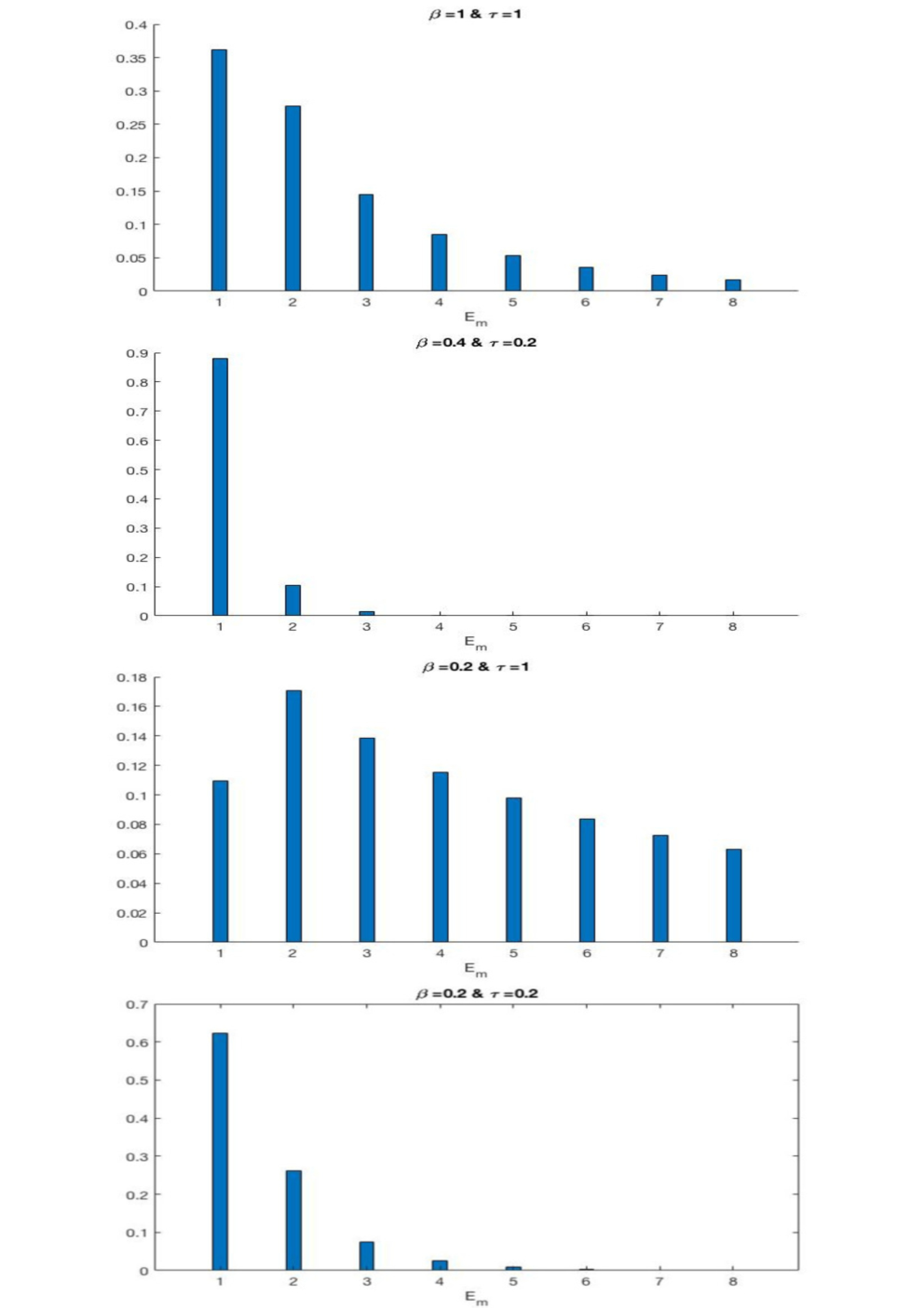
To give a concrete illustration, in Fig. IV, reprinted with permission from Al-Naseri-2021 copyright 2021 by the American Physical Society, we show a bar chart for the normalized number density in the different energy states, for a few values of the temperature and magnetic field, under the assumption that the density is low enough for the system to be non-degenerate, i.e. assuming .
As a result of the background dependence, Eq. (108), in the Landau quantized regime, the electrons behave as a multi-species system, where each particle species has its own rest mass, as given by Eq. (103) but with . This is because the separation between Landau levels is of the order of the rest mass, and all excitations by quanta with energies of that order have been neglected. If we define the effective number density of each ”species” (discrete energy-state) as
| (110) |
we see that to a large degree will be determined by the Boltzmann factors of Eq. (104). For a study of Langmuir waves in a Landau quantized plasma, see Ref. landau-quant.
While we have here focused on the extreme case of relativistic Landau quantization, we note that the thermodynamics is much affected also in the non-relativistic regime, provided the Zeeman energy is of the same magnitude or larger than the characteristic kinetic energy in the background plasma. For applications of Landau quantization in the non-relativistic regime, see e.g. LQ1; LQ2
V.3 Nonlinear effects
Not surprisingly, quantum kinetic models can describe a great variety of nonlinear phenomena. Just like for classical plasmas, a fair share of these phenomena is induced by the ponderomotive force. For example, the ponderomotive force is the driver of plasma wake field generation Wakefield, the key mechanism in soliton formation Soliton, and the main source of nonlinear self-focusing Selffocusing. While the main features of classical and quantum kinetic models driven by the ponderomotive force are similar, nevertheless there are important differences. For one thing, in a magnetized plasma, the classical ponderomotive force have cyclotron resonances Karpman. In quantum kinetic theory, the classical terms are still present, but they are complemented by terms containing extra quantum resonances PRL2010; PRE2011.
The concept of a ponderomotive force in quantum kinetic theory is not as straightforward as in a fluid theory. Depending on definition, some low-frequency nonlinearities induced by quadratic nonlinearities may be included as a ponderomotive force term or not. In order to avoid ambiguities, we will focus on the regime where the phase velocity of the high-frequency wave is much higher than the thermal velocity (or characteristic velocity, in case of degeneracy effects).
As a starting point, we will base our study on the long-scale version of the model put forward in Section III, that is, Eq. (66). Next, we consider circularly polarized electromagnetic waves of high frequency propagating parallel to an external magnetic field, , and use the following ansatz
| (111) |
The amplitudes are assumed to vary much slower than the exponential phase factors, and the star denotes complex conjugates. Since the basic wave modes propagating parallel to are either left- or right-circularly polarized, we have . Furthermore, all perturbations are small, such that weakly nonlinear perturbation theory is applicable, and we will focus on the ponderomotive contribution, that is the quadratically nonlinear low-frequency terms.
In order to calculate the weakly nonlinear low-frequency response to an incoming transverse wave packet we make the ansatz
| (112) |
where is the background distribution, is a low-frequency part due to quadratic nonlinearities and is a slowly modulated high-frequency wave. The background distribution will be taken to be of the form
| (113) |
where is the equilibrium density, the thermal velocity is defined as . It should be stressed that the background distribution (113) has been picked mostly for convenience. In fact, the results below are not depending sensitively on the background, as long as the phase velocity is larger than the characteristic velocity. For example, a degenerate distribution, but with the Fermi velocity smaller than the phase velocity would produce identical results.
Given the ansatz (111) and (112), the aim is then to find an equation for the low-frequency part of the distribution function. From such an equation we can then calculate the low-frequency response in the current density and magnetization, and compare with the results for a ponderomotive force, as defined from a fluid theory. First we deduce the high-frequency linear perturbation of the distribution function, which is given by ( for left-hand (right-hand) circularly polarized waves. The expressions for found from Eq. (66) to linear order can be easily computed from Eq. (9) in Ref. Lundin2010, and the result is
| (114) |
Next, allowing for slow modulations and solving the equation to first order in , , we note that the zero-order solution applies after making the substitution and in Eq. (114), and then expanding to first order in the slow derivatives. Inserting the ansatz above into the evolution equation and consider the slow-time scale and keeping only up to quadratic nonlinearities we obtain the equation
| (115) | |||||
where c.c. stands for complex conjugate. Here we have also added a low-frequency electric field in the -direction, , which has as source. Equations (115) and (114) now constitute a basis for calculating the nonlinear response in the current density and magnetization.
After some algebra (described more closely in Ref. PRE2011), based on the low-frequency part of Ampere’s law, we end up with the final expression for the induced low-frequency field, which can be written in terms of the ponderomotive force as
| (116) |
where can be divided into its classical and its spin contribution according to
with the different parts given by
| (117) |
and
| (118) |
The classical ponderomotive term (117) agree with an expression first derived by Ref. Karpman. The spin ponderomotive term (118)was first derived in Ref. PRE2011. Our spin term agree with that work, although - in contrast to that expression - we have integrated the contribution over the spin-up and the spin-down term. Note that although the modest scale lengths assumed tend to limit the magnitude of the spin terms, the quantum contribution can still be larger or comparable to the classical terms, in particular close to resonances or . Note that due to the closeness of the spin-precession frequency and the cyclotron frequency , these resonances can be more or less overlapping.
An interesting feature of the above expression is the second term in (118), containing the factor. If we had not averaged over the spin states, spin-up and spin-down electrons would be affected in opposite direction (recall that we get the factor from the difference in the number of spin-up and down particles), and hence a part of the spin contribution to the ponderomotive force leads to a spin-polarization being induced by the high-frequency wave. We will not explore the consequences of the expression (118) further, however, but refer to Refs PRL2010; PRE2011; PRE2010; POP2010 that have studied various types of nonlinear dynamics induced by the spin ponderomotive force.
Before ending the description of spin ponderomotive physics, it is worth noting that in certain cases, weakly relativistic contributions, in particular the spin-orbit correction, can be important for the end result. To explore this fact, we will make use of the weakly relativistic limit of Eq. (84). obtained by letting . This model was first derived by Ref. Asenjo-2012, and is given by
| (119) |
While we still use put gamma factors to unity (or ), the model keep terms linear in a -expansion, such that Thomas precession, spin-orbit terms, and a non-trivial velocity-momentum relation (including spin) is kept. Taking the appropriate limit, the source terms used in Section III is replaced by
| (120) | ||||
| (121) |
Here is the free charge density and the free current density, the polarisation and magnetisation are given by
| (122) | ||||
| (123) | ||||
| (124) |
Next, we make the same calculation as for the simpler (non-relativistic) model (given by Eq. (66)), considering a quasi-monchromatic circularly polarized electromagnetic wave. However, to reduce the algebra we consider a non-magnetized plasma, i.e. we let . We refer the reader to Ref. POP2013 for the algebraical details, and move on to the end result for the ponderomotive force.
| (125) |
where, due to the technicalities of the model, we have a result for the time-derivative of the ponderomotive force, rather than the ponderomotive force itself. The expression is
| (126) |
The last term is the classical contribution, and the second to last term in the square bracket is what is obtained without the weakly relativistic effects. However, if we assume that is roughly of order unity, we see that all terms in the square brackets are of the same order. This implies that when dealing with an unmagnetized plasma where spin effects are important, the spin orbit coupling contributions must be taken into account as well. However, the previous result for the ponderomotive force, Eq. (118) is still relevant, as spin terms tends to be more important in magnetized plasmas, and hence the simpler model (66) can still be justified.
VI The full Dirac theory - the DHW equations
Quantum relativistic treatments are of interest in several different contexts QRP-1; QRP-2; QRP-3. Dense astrophysical objects can have a Fermi energy approaching or exceeding the electron rest mass energy, the strong magnetic fields of magnetars give rise to relativistic Landau quantization . Importantly, the continuous evolution of laser intensity brings a variety of quantum relativistic phenomena accessible to experimentalists. Upcoming laser facilities of interest in this context include, e.g., the extreme light infrastructure (ELI) Eli; Dunne and the European x-ray free electron laser (XFEL) XFEL; Ringwald,
The quantum kinetic models of previous sections has all made various simplifications as compared to the full quantum relativistic theory. In particular, in order to avoid the mixed electron-positron states of the Dirac theory, up to now we have imposed limitations on the electric field. Specifically, we have demanded where is the critical field, in order to avoid the complications associated with significant pair-production due to the Schwinger mechanism. In this section, however, we will take on the full complexity of the Dirac theory using the so called Dirac-Heisenberg-Wigner (DHW) formalism BB-1991. Compared to previous sections, new features of the theory includes, Zitterbewegung (a rapid (speed of light) particle motion associated with interference between positive and negative energy states), vacuum polarization, and electron-positron pair creation. Also, the previous 2 by 2 Wigner matrix will be replaced by 16 components, due to the 4 components of the Dirac spinors. Nevertheless, many other aspects of the quantum kinetic theory will be familiar and we will point out how the DHW-formalism can be related to the quantum-kinetic approximations presented earlier.
VI.1 The DHW-model
The DHW-model was first derived by Ref. BB-1991. Moreover, some relatively minor variations of this derivation has been published in the literature more recently, see e.g. Gies; Sheng. As all these treatments are fully satisfactory, we will not repeat the calculations, but just point out a few of the main features.
- 1.
The derivation is based on the Dirac equation, which gives the time evolution of Dirac four spinors, generally describing mixed electron positron states.
- 2.
Just like in previous theories, a gauge-invariant Wigner transformation is made, which here produce a 4 by 4 Wigner matrix, with the components depending on phase-space variables just like in standard kinetic theory.
- 3.
The main omission is made when using the Hartree-approximation where the electromagnetic field is treated as a non-quantized field. This approximation amounts to neglecting the quantum fluctuations. We will come back to the consequences of this approximation.
- 4.
In order to write the equations in a physically more transparent form, the 16 components of the Wigner matrix is decomposed into 4 different four vectors, which in turn is split into temporal and spatial components. Most of these quantities have a clear physical meaning, which helps forming a physical understanding of the theory.
- 5.
The (phase-space) current density and charge density are parts of the DHW-functions, which makes it straightforward to close the system using Maxwell’s equations.
With these preliminaries, we jump directly to the DHW-equations, which in units where can be written in the form:
| (127) |
Due to the Wigner transform, we cover short-scale quantum phenomena in much the same way as in the previous sections. This is illustrated by the appearance of the non-local operators in Eq. (127), which are given by
| (128) | ||||
| (129) | ||||
| D | (130) | |||
| (131) |
As before, the operators reduce to their local approximations (i.e. , , , and ) for scale lengths much longer than the characteristic de Broglie length.
To close the system, we need the source terms in Maxwell’s equations, which are given by
| (132) |
and
| (133) |
Thus is the time component of the four-vector phase space function that gives the four current density, and is the spatial component, i.e. the current density. Most, if not all, DHW-functions have fairly concrete interpretations which helps guiding the physical intuition. To gain a better understanding, we take a look at some of the conserved quantities of the DHW-system (for a derivation, see Ref. BB-1991). Firstly, the total energy is given by
| (134) |
secondly, the linear momentum is
| (135) |
and, finally, the total angular momentum M is
| (136) |
We can see in Eq. (134) that the current density can be related to the kinetic energy, as expected. However, the role of mass density is played by another function , with no trivial relation to the charge density. As the Dirac field contain both electrons and positrons, the lack of a simple relation between the mass density and the charge density should not be surprising. Nevertheless, in the expression for momentum (135), we see that acts as a phase space momentum density. Since electrons and positrons contribute with opposite signs to , we realize that electrons and positrons must have a different dependence on . To be concrete, for electrons and positrons moving in the same direction, we need to shift the momentum dependence for the dependent variables according to , as will be illustrated more explicitly below. This is not an issue when solving the DHW-equations, as the DHW-variables generally describe coupled electron and positron states anyway. However, this insight can be of some importance e.g. when interpreting results, in particular when numerical calculations have been made. The shift in momentum dependence is consistent with the common interpretation of positrons as being electrons moving backwards in time.
Another observation that can be made based on the conserved quantities is that the term can be identified as the spin contribution to angular momentum, i.e. gives the spin density. Finally, the equation for in Eq. (127) shows a division of the total current density into its free part, magnetization part, and polarization part. To be specific, we can deduce that gives the magnetization, and gives the polarization. For some further discussion of the physical interpretation of the DHW-functions, see Ref. BB-1991.
Contrary to previous kinetic theories, in the DHW-formalism, the kinetic variables are not zero even in vacuum, in older terminology we would say that the vacuum is filled with the particles of the Dirac sea. However, in the absence of a spin polarizing magnetic field, the only DHW-functions with nonzero vacuum-values are the mass density and current density, which are given by
| (137) |
where . The expressions above are obtained by calculating the Wigner operator for the free particle Dirac equation and taking the vacuum expectation value. Note that while the charge density is zero (due to the cancellation of the electron and positron vacuum fluctuations), the same is not true for the current density. The reason is that there are two signs that enter the picture - firstly electrons and positrons have opposite signs of the charge, but secondly, switching electrons for positrons means letting , such that the vacuum contributions are additive. Nevertheless, when integrating over momentum to get the total current density, we still get zero as one would expect. The substitution when switching between electrons and positrons also holds for real particles as well as the vacuum contribution. In particular, for beam systems, this is important to keep in mind, as is illustrated in Fig. 5.
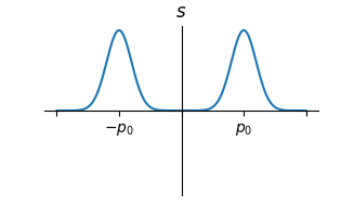
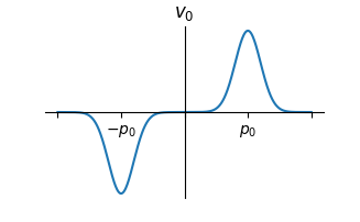
When adding the real particles of the Dirac field (electrons and/or positrons) into the picture, we can add distribution functions much like in the theories of the previous sections. Specifically, we could start from a background
| (138) |
with a nonzero charge density
| (139) |
The function can be picked as any common background distribution function from classical kinetic theory, i.e. a Maxwell-Boltzmann, Synge-Juttner, or Fermi-Dirac distribution, depending on whether the characteristic kinetic energy is relativistic and whether the particles are degenerate.
Note that for a completely degenerate () Fermi-Dirac background of electrons (and no positrons ), the electron and vacuum contributions for the mass density and current density cancel inside the Fermi sphere. Consequently, for momenta , where is the Fermi momentum, we have . Furthermore, note that in the presence of a strong field in the background state (e.g. a strong constant magnetic field), these fairly simple background expressions need to be modified. For example, in a case with , also the vacuum states will be subject to Landau quantization. Moreover, the spin density and magnetization (as described by the functions and , respectively) will no longer vanish in the background state, due to the contribution from real particles.
VI.2 The electrostatic one-dimensional case
In order to illustrate some features of the DHW-theory, we will consider the case of a one-dimensional electrostatic field, i.e. . At the same time, the DHW-functions depend on , but where the momentum dependence can be reduced to two independent variables (), due to the rotational symmetry.
Due to the simplified geometry, only half of the 16 scalar DHW-functions will be nonzero. Moreover, only four of these variables will be independent. There are different ways of finding these nonzero-variables. Here we will just present the result, which is straightforward to verify by direct substitutions into the DHW-equations, Eq. (127). For a more systematic derivation of the reduced electrostatic equations, see Ref. Al-Naseri-2021. As it turns out, the DHW-equations can be expressed in terms of four variables , related to the original DHW-functions as follows:
| (140) | ||||
where . Taking this as an ansatz for the variables and substituting the expressions into Eq. (127), we obtain the electrostatic equations:
| (141) | ||||
where, in the 1D-case of study, The above system is closed by Ampére’s law, which in terms of the -variables is written
| (142) |
While Eqs. (VI.2)-(142) represent a huge simplification compared to the full DHW-theory, they can still describe a host of different phenomena. As an example, Ref. Gies2 has used a similar set to study Schwinger pair-production for given electrostatic pulses. From a plasma physics perspective, studies of Langmuir waves in a high density plasma is a natural problem. While the nonlinear strong field regime is interesting to study (allowing for the Schwinger mechanism), we leave that for a future numerical investigation. Instead we will focus here on the problem of linearized Langmuir waves, as this is straightforward to study analytically.
The nonzero background quantities for the -variables can be written as
| (143) | ||||
using upper index for the unperturbed background values, and letting the variables have both electron and positron contributions. Next, we divide the variables into unperturbed and perturbed variables according to
| (144) |
(with and only a perturbed electric field ) and linearize (VI.2) and (142). Making use of the relation
| (145) |
the problem is reduced to linear algebra. Solving for , and restoring to identify the quantum contributions (e.g. letting in the denominator of Eq. (142)), we obtain
| (146) | ||||
| (147) | ||||
| (148) | ||||
| (149) |
where
| (150) | ||||
| (151) |
Note that and depend on the full momentum, but we suppressed the perpendicular momentum to simplify the notation. Combining the above results for with Ampere’s law (142) we obtain the dispersion relation with
| (152) |
The classical, but relativistic, limit of the dispersion relation is obtained by letting . Taking this limit, the dispersion function (152) reduces to
| (153) |
which can be shown to agree with the standard result after some straightforward algebra. Note that the appearance of in the integration measure is just a matter of normalization, and not a sign of any remaining quantum features.
The main purpose here as been to demonstrate the usefulness of the DHW-equation for practical plasma calculations. However, before ending the discussion, without going into details, let us point out a few features of the general dispersion relation.
- 1.
Apart from the effect of a relativistic Fermi velocity, in the relativistic regime, the quantum contribution to the real part of the plasma frequency will actually decrease with increasing density, since quantum terms are compared with the (high) relativistic Fermi energies and Fermi momenta.
- 2.
The main new effect due to the quantum relativistic regime, comes from the new types of resonant denominators, associated with wave damping. In particular, even for we may still have a resonant denominator (corresponding to electron-positron pair-production), provided the pair-creation condition is fulfilled.
- 3.
Due to the vacuum background, the integrand is nonzero even in the absence of particles, giving raise to the effect of vacuum polarization contribution. While this term typically gives a contribution that is much smaller than that from the real particles, the given expression is subject to ultra-violet divergences that must be handled using a renormalization scheme, see e.g. Ref. BB-1991.
Naturally, the above points only give the principal features. A more thorough study of the quantum relativistic dispersion relation for Langmuir waves has to be done numerically. This will be the subject of a future paper.
VI.3 Limiting cases of the DHW-theory
Apart from exchange effects, the DHW-equations covers all the physical phenomena presented in previous sections. Thus, ideally, we should be able to recover all the previous models, (except the parts presented in section III) as special cases of the DHW-formalism. However, demonstrating the equivalence in appropriate limiting cases is somewhat non-trivial. First of all, the DHW-equations do not only describe electrons, since a Foldy-Wouythuysen transformation cannot be made in the fully quantum relativistic regime. Furthermore, the equations with a spin-dependent Wigner-function uses a Q-transform to get a scalar theory, which further complicates a comparison. Nevertheless, though a complete investigation is yet to be made, showing the equivalence of the DHW-formalism with the models of section IV (i.e. the non-relativistic Pauli-limit) is relatively straightforward.
First, we note that for fields well below the critical field, there is little ambiguity whether we have electron or positron states. Considering the case of electrons only, ignoring relativistic effects, the charge and mass density are the same (due to the normalization, the constant factors involving and do not enter), i.e. . As a first exercise, let us recover the model based on the Schrödinger Hamiltonian. This implies dropping the effects of the electron spin, i.e. the spin density, magnetization, and spin polarization are zero, and thus we let in the DHW-equations. As a result of the above approximations, we get , which immediately lead to a closed equation for :
| (154) |
Identifying with the Wigner function of section II, using the definitions of the nonlocal variables to write the more explicitly, Eq. (154) gives us
| (155) |
The definitions of , etc., are the same as those in section II. We note that Eq. (155) coincides with Eq, (36). Thus Eq. (155) generalizes the results for the electrostatic version of the Schrödinger Hamiltonian to also cover electromagnetic fields, as follows naturally using the gauge-invariant Wigner transform, as discussed in section II.3. Alternatively, we could re-derive the same equation by dropping the spin terms in Eq. (61) (all terms proportional to ), and integrate the equation over spin space.
Next, our aim is to recover the model of Section IV, based on the Pauli Hamiltonian. As the short scale physics associated with the non-local expressions (128)-(131) has already been established above, for convenience we restrict ourselves to the case of long scale lengths (), such that the local approximations (i.e. dropping the variables with tilde) can be used. For the non-relativistic case, we can still put the charge and mass density equal, i.e. . Secondly, in the absence of relativistic effects (and for the given normalizations) and for the case of electrons only, the spin density and the magnetization is the same, i.e. . Thirdly, a non-vanishing polarization due to the spin only enters in the relativistic theory, and thus we can put . Finally, the term in Eq. (127) is a small correction (in a quantum relativistic expansion ), and hence we can use the approximation . With these simplifications as a starting point, the DHW-equations can be combined to give the following evolution equation for the magnetization:
| (156) |
Normally, we should drop the term , since such a term is identically zero. However, recall that before introducing approximations, this term would rather be proportional to . As it turns out, the local approximations are applicable everywhere else, as in those cases, the corrections are compared with larger surviving terms. Here, however, we need to use the full expression , and evaluate the term to the first non-vanishing order in an expansion in the small parameter . Performing this expansion and identifying with and with , after some algebra we can confirm the exact agreement of Eq. (156) with Eq. (73).
Next, to establish agreement with the model based on the Pauli Hamiltonian, we need to re-derive Eq. (72). Using the same approximations as before, we immediately get
| (157) |
While there is a litle bit of algbra involved (since the operator contains the magnetic field), it is straightforward to show that Eq. (157) reduces to Eq. (72). Finally, we note that the current sources to be used in the DHW-equations are the same as in the Pauli-limit, given that polarizations currents are dropped in non-relativistic theory. Furthermore, as the agreement between Eqs. (72)-(73) and (66) has already been established, and the short-scale physics (as described by Eq. (155)) have been recovered, for most practical purposes, the full model based on the Pauli Hamiltonian (Eq. (52)) have also been verified, although not in a strict sense.
While the above confirmation is reassuring, the main purpose of studying approximate versions of the DHW-model is to find models that are easier to analyze in specific cases. The DHW-equations allow for systematic expansions in numerous quantum and relativistic parameters, , (where represents electric and/or magnetic fields), , , and to name a few. Here and represents general temporal and spatial scales, rather than specific frequencies and wave numbers. Depending on the ordering of the dimensionless parameters, there are several possibilities for approximate models containing different combinations of expansion parameters. A systematic search for consistent approximations of the DHW-system is a project for further research.
VII Concluding remarks
While the aim of this review has been to cover many aspects of quantum kinetic theory, naturally, there are many interesting and important topics that we have not touched upon. While, undoubtedly, many things will be left out altogether, let us here at least partially remedy some of the omissions mad, by pointing to a few relevant aspects of quantum kinetic theory that we have not covered.
Firstly, as is well-known, there are close connections between hydrodynamic and kinetic theories. In particular, a common approach to derive accurate fluid theories is by making moment expansions of kinetic theories. In a quantum context, this scheme has been used to derive fluid theories from kinetic theories e.g. by Refs. Momexp1; Momexp2; Momexp3 for the model defined by the Schrödinger Hamiltonian and by Refs. Manfredi-spin1; Momexp4 for the Pauli Hamiltonian model, and also by Ref. Hurst-2017 for the model where the Pauli-Hamiltonian is extended by the spin-orbit term. Moreover, moment expansion for models including exchange effects has been made by e.g. Refs. Haas-exchange; Manfredi_DFT.
Secondly, we note that for completely degenerate systems, in certain cases kinetic models may be simplified. This happens in situations when the phase-space density is conserved, in which case the dynamics is determined by the Fermi surface. This has been explored in so called waterbag models of plasmas Manfredi_DFT; Waterbag and also for the case of a semiclassical model based on the Pauli Hamiltonian Brodin-Stefan.
Thirdly, we stress that we here have focused on non-dissipative quantum kinetic models, ignoring the effects of higher order correlation in the BBGKY-hierarchy, neglecting all the influence of collisions. The effect of dissipation is a research topic in its own right, of particular importance in the strong coupling regime. For references covering this field, see e.g. Bonitz-book; Ichimaru82; Bonitz2015.
As our review has focused on quantum kinetic models, and the worked out examples has served the purpose of illustrating the applicability of the theory, many aspects of quantum kinetic theory have still been ignored. In particular interesting theoretical aspects involving wave-particle interaction, spin-polarization dynamics, numerical computation schemes, and the interesting interplay with single particle dynamcis QRR
Appendix A BBGKY-Hierarchy and the Mean-Field Approximation
The -particle density matrix is not directly applicable in the case where we have a large number of particles, as is typically the case for plasmas. It is therefore necessary to make some approximations to reduce the complexity of the equations. One commonly used approximations when dealing with plasmas is the mean-field approximation, which we will consider here. Since it is more convenient for this type of considerations, we will here use the operator representation of the density matrix (as opposed to using the position representation as was done in Section II. Using the bra-ket notation we can define the density operator as
| (158) |
where are -particle states. The evolution equation can then be written as
| (159) |
where denotes the commutator. Assume that we have an Hamiltonian in the form
| (160) |
where
| (161) |
is the kinetic energy operator, with being the momentum operator acting on the :th particle. The operator in the last term corresponds to particle-particle interactions, which we will later take as the Coulomb interaction. However, for now, we only need to assume that the interaction is symmetric under exchange of particles, i.e., . We note that the density matrix is symmetric with respect to change of particles, i.e.,
| (162) |
This is true, as long as the particles are indistinguishable, and hence both for fermions and bosons. We may now define the -particle reduced density matrix as
| (163) |
where we, for convenience, have multiplied by the number of particles times. Now, using the above we can derive the so called BBGKY-hierarchy for the reduced density matrices:
| (164) |
Here we have assumed that is large so that we may use to any order where the above equation is of any practial use. We note that the one-particle density matrix couples to the two-particle density matrix, etc. Now, we are only interested in the lowest equation which is
| (165) |
In order to make progress from this, we write the two-particle density matrix as
| (166) |
where is the two-particle correlations defined by the equation above. In the lowest order approximation, we completely neglect the two-particle correlations . We then get the so-called mean-field, or Hartree approximation
| (167) |
We note that the normalisation of the density matrix is such that
| (168) |
i.e., the number of particles. The diagonal elements can then be identified as the local density of particles . In particular, in the case of a plasma interacting via the Coulumb interaction
| (169) |
and the last term is
| (170) |
where the last step is written in terms of the mean-field potential, i.e., the potential created by all particles interacting with particle 1. Here we have only considered particles which are indistinguishable, but we have not yet taken into account the correct symmetry. For fermions, we need to modify the procedure slightly in order to account for the antisymmetry of the wave function, but the basic principle is the same. We will do this modification in Section III where we consider exchange effects. The conclusion from the above considerations is that if we can assume that particle correlations are negligible, we may describe the plasma as particles moving in the mean-field created by all the other particles.
References
- (1) G. Manfredi, H. Paul-Antoine, and H. Jérôme, Rev. Mod. Plasma Phys. 3, 13 (2019).
- (2) P. K. Shukla and B. Eliasson Rev. Mod. Phys. 83, 885 (2011).
- (3) D. B. Melrose, Rev. Mod. Plasma Phys. 4, 8 (2020).
- (4) S. V. Vladimirov and Yu O. Tyshetskiy Phys.-Usp. 54 1243 (2011).
- (5) P. K. Shukla and B Eliasson Phys.-Usp. 53 51 (2010).
- (6) F. Haas Quantum Plasmas, A Hydrodynamics Approach, Chap 2 (Springer, New York, 2011)
- (7) N. Crouseilles G. Manfredi, Computer Phys. Commun. 185 448 (2014).
- (8) F. Haas and P. K. Shukla, Phys. Plasmas. 15 112302 (2008).
- (9) F. Haas, B. Eliasson, P. K. Shukla, and G. Manfredi Phys. Rev. E 78, 056407 (2008).
- (10) Yu. Tyshetskiy, S. V. Vladimirov, and R. Kompaneets, Phys. Plasmas 21, 122114 (2014).
- (11) Yu. Tyshetskiy, S. V. Vladimirov, and R. Kompaneets, J. Plasma Phys. 79, 387 (2013).
- (12) N. Crouseilles, P.-A. Hervieux, and G. Manfredi, Phys. Rev. B 78, 155412 (2008).
- (13) F. Haas, Contrib. Plasma. Phys. e202100046 (2021).
- (14) P. A. Andreev, Annals Phys. 350, 198 (2014).
- (15) J. Zamanian, M. Marklund, and G. Brodin, Phys. Rev. E 88, 63105 (2013).
- (16) J. Zamanian, M. Marklund, and G. Brodin, Eur. Phys. J. D 69, 25 (2015).
- (17) R. Ekman, J. Zamanian, and G. Brodin, Phys. Rev. E 92 013104 (2015).
- (18) G. Brodin, R. Ekman, and J. Zamanian,, Phys. Plasmas 26, 092113 (2019).
- (19) J Hurst, O. Morandi, G. Manfredi, et al. Eur. Phys. J. D 68, 176 (2014).
- (20) G. Brodin, M. Marklund, J. Zamanian, A. Ericsson, and P. L. Mana, Phys. Rev. Lett. 101, 245002 (2008).
- (21) J. Zamanian, M. Marklund, G. Brodin, New J. Phys. 12, 043019 (2010)
- (22) P. A. Andreev, Phys. Plasmas 23, 062103 (2016).
- (23) P. A. Andreev, Phys. Plasmas 25, 032116 (2018).
- (24) P. A. Andreev and L. S. Kuzmenkov, Phys. Plasmas 24, 112108 (2017).
- (25) P. A. Andreev, Phys. Plasmas 24, 022115 (2017).
- (26) F. A. Asenjo, J. Zamanian, M. Marklund, G. Brodin and P. Johansson, New J. Phys. 14, 073042 (2012).
- (27) J. Hurst, P. A. Hervieux, and G. Manfredi, Phil. Trans. R. Soc. A. 375 20160199 (2017).
- (28) R. Ekman, H. Al-Naseri, J. Zamanian, and G. Brodin. Eur. Phys. J. D 75, 29 (2021)
- (29) R. Ekman, F. A. Asenjo, and J. Zamanian, Phys. Rev. E 96, 023207 (2017).
- (30) R. Ekman, H. Al-Naseri, J. Zamanian, and G. Brodin, Phys. Rev. E 100, 023201 (2019).
- (31) I. Bialynicki-Birula, P. Gornicki, and J. Rafelski, Phys. Rev. D 44, 1825 (1991).
- (32) H. Al-Naseri, J. Zamanian, R. Ekman and G. Brodin, Phys. Rev. E 102, 043203 (2020).
- (33) H. Al-Naseri, J. Zamanian, and G. Brodin, Phys. Rev. E 104, 015207 (2021).
- (34) F. Hebenstreit, R. Alkofer, and H. Gies, Phys. Rev. Lett. 107, 180403 (2011).
- (35) X. L. Sheng, R. H. Fang, Q. Wang, and D. H. Rischke, Phys. Rev. D 99, 056004 (2019).
- (36) I. A. Aleksandrov and C. Kohlfurst, Phys. Rev. D 101, 096009 (2020).
- (37) J. T. Mendonça, Symmetry, 13, 1361, (2021).
- (38) M. Bonitz, Quantum kinetic theory, 2nd edn. (Springer, Cham, 2016)
- (39) S. A. Wolf, D. D. Awschalom, R. A. Buhrman, J. M. Daughton, S. Von Molnar, M. L. Roukes, A. Y. Chtchelkanova, and D. M. Treger, Science 294, 1488 (2001).
- (40) H. A. Atwater, Sci. Am. 296, 56 (2007).
- (41) A Moradi, J. Phys.: Condens. Matter 21 045303 (2008).
- (42) G. Manfredi and P.-A. Hervieux, Appl. Phys. Lett. 91, 61108 (2007).
- (43) D. Liu et al. Nat. Commun. 9, 193 (2018).
- (44) G. Chabrier, F. Douchin, and A. Potekhin, J. Phys. Condens. Matter. 14, 9133 (2002).
- (45) D. A. Uzdensky and S. Rightley, Rep. Prog. Phys. 77, 036902 (2014).
- (46) S. H. Glenzer and R. Redmer, Rev. Mod. Phys. 81, 1625 (2009).
- (47) L. C. Thomas, T. Dezen, E. B. Grohs, and C. T. Kishimoto, Phys. Rev. D, 101, 063507 (2020).
- (48) D. Del Sorbo, D. Seipt, T. G. Blackburn, A. G. R. Thomas, C. D. Murphy, J. G. Kirk, and C. P. Ridgers, Phys. Rev. A 96, 043407 (2017).
- (49) D. D. Sorbo, D. Seipt, A. G. R. Thomas, and C. P. Ridgers, Plasma Phys. Controlled Fusion 60, 064003 (2018).
- (50) Y.-F. Li, R. Shaisultanov, K. Z. Hatsagortsyan, F. Wan, C. H. Keitel, and J.-X. Li, Phys. Rev. Lett. 122, 154801 (2019).
- (51) A. K. Harding and D. Lai, Rep. Prog. Phys. 69, 2631 (2006).
- (52) E. Wigner, Phys. Rev. 40, 749 (1932).
- (53) J. J. Sakurai, and J. Napolitano, Modern Quantum Mechanics, 2nd edn. (Cambridge University Press, Cambridge, 2017)
- (54) J. E. Moyal, Math. Proceed. Cambridge Phil. Soc. 45, 99, (1949).
- (55) C Zachos, D Fairlie, and T Curtright, Quantum Mechanics in Phase Space (World Scientific, 2005).
- (56) B. Eliasson, and P. K. Shukla, J. Plasma Phys 76, 7 (2009).
- (57) G. Manfredi, Fields Inst. Commun. 46, 263, (2005).
- (58) R. L. Stratonovic, Zh. Eksp. Teor. Fiz. 58, 1612 (1970) [Sov. Phys. -JETP 31, 864 (1970).
- (59) O. T. Serimaa, J. Javanainen, and S. Varró, Phys. Rev. A 33, 2913 (1986).
- (60) A. H. MacDonald and Garnett W. Bryant Phys. Rev. Lett. 58, 515 (1987).
- (61) D. B. Boercker and J. W. Dufty, Ann. Phys. 119, 43 (1979).
- (62) S. J. Wang and W. Cassing, Ann. Phys. 159, 328 (1985).
- (63) O. Von Roos and J. Zmuidzinas, Phys. Rev. 121, 941 (1961).
- (64) T. J. M. Boyd, and J. J. Sanderson, The Physics of Plasmas (Cambridge University Press, Cambridge 2003).
- (65) N. N. Bogolyubov Zh. Eksp. Teor. Fiz. 16, 691 (1946); [JETP 10, 265 (1946)].
- (66) M. O. Scully and K. Wódkiewicz, Found. Phys. 24, 85 (1994).
- (67) G. Manfredi and Jerome Hurst, Plasma Phys. Control. Fusion 57 054004 (2015).
- (68) N. Crouseilles, P. Hervieux, Y. Li, G. Manfredi, and Y. Sun, J. Plasma Phys., 87, 825870301, (2021).
- (69) G. Swanson, Plasma Waves (Taylor & Francis, 2003).
- (70) J. Lundin and G. Brodin, Phys. Rev. E 82, 056407 (2010)
- (71) A. Hussain, M. Stefan, and G. Brodin, Phys. Plasmas 21, 032104 (2014)
- (72) F. Haas, Phys. Plasmas 15, 022104. (2008)
- (73) S. Rightley, D. Uzdensky. J. Plasma Phys. 84 905840408. (2018).
- (74) Foldy and Wouthuysen, Phys. Rev. 78, 29 (1950).
- (75) A. J. Silenko, Phys. Rev. A 77 012116 (2008).
- (76) W. Shockley and R. P. James, Phys. Rev. Lett. 18, 876 (1967).
- (77) W. Shockley, Phys. Rev. Lett. 20, 343 (1968).
- (78) S. Coleman and J. H. Van Vleck, Phys. Rev. 171, 1370 (1968).
- (79) D. Babson, S. P. Reynolds, R. Bjorkquist, and D. J. Griffiths, Am. J. Phys. 77, 826 (2009).
- (80) D. B. Melrose and A. J. Parle, Aust. J. Phys. 36, 755 (1983).
- (81) S. Eliezera, P. Norreys, J. T. Mendonça, and K. Lancaster, Phys. Plasmas 12, 052115 (2005).
- (82) M. I. Shaukat, Phys. Plasmas 24, 062305 (2017).
- (83) T Tajima, JM Dawson Physical Review Letters 43 (4), 267.
- (84) P. K. Shukla, N.N. Rao, M. Y. Yu and N. L. Tsintsadze, Phys. Reports, 138, 1 (1986).
- (85) T. Kurki-Suonio, P. J. Morrison, and T. Tajima Phys. Rev. A 40, 3230, (1989).
- (86) V.I. Karpman and H. Washimi, J. Plasma Phys. 18 , 173 (1977).
- (87) G Brodin, A. P. Misra, M Marklund Phys. Rev. lett. 105, 105004 (2010).
- (88) M. Stefan, J. Zamanian, G. Brodin, A. P. Misra, M- Marklund, Phys. Review E 83, 036410 (2011).
- (89) A.P. Misra, G. Brodin, M. Marklund, and P. K. Shukla Physical Review E 82, 056406 (2010).
- (90) A.P. Misra, G. Brodin, M. Marklund, and P. K. Shukla Phys. Plasmas 17, 122306 (2010).
- (91) M. Stefan and G. Brodin, Phys. Plasmas 20, 012114 (2013).
- (92) P. Zhang, S. S. Bulanov, D. Seipt, A. V. Arefiev, and A. G. R. Thomas, Phys. Plasmas 27, 050601 (2020).
- (93) I. S. Elkamash, F. Haas, and I. Kourakis, Phys. Plasmas 24, 092119 (2017).
- (94) Y. Shi, J. Xiao, H. Qin, and N.J. Fisch, Phys. Rev. E 97, 053206 (2018).
- (95) http://www.extreme-light-infrastructure.eu/.
- (96) G. Dunne, Eur. Phys. J. D 55, 327 (2009).
- (97) http://xfel.eu.
- (98) A. Ringwald. Phys. Lett. B 510, 107 (2001).
- (99) F. Hebenstreit, R. Alkofer, and H. Gies. Phys. Rev. D 82, 105026 (2010).
- (100) Z. Cai, Y. Fan, R. Li, T. Lu, and Y. Wang J. Math. Phys. 53, 103503 (2012);
- (101) F Haas, M. Marklund, G. Brodin, and J. Zamanian, Phys. Lett A, 374, 481, (2010).
- (102) F Haas, M. Marklund, G. Brodin, and J. Zamanian, NJP, 12, 073027, (2010).
- (103) J Zamanian, M Stefan, M Marklund, and G Brodin, Phys. Plasmas 17, 102109 (2010).
- (104) G. Manfredi, J. Plasma Phys. 86, 825860201, (2020).
- (105) G. Brodin and M. Stefan, Phys. Rev. E 88, 023107 (2013).
- (106) S. Ichimaru Rev. Mod. Phys. 54, 1017 (1982).
- (107) M. Bonitz, N. Schlunzen, and S. Hermanns, Contrib. Plasma Phys. 55, 152 (2015).
- (108) V. Dinu, C. Harvey, A. Ilderton, M. Marklund, and G. Torgrimsson, Phys. Rev. Lett. 116, 044801 (2016).