![[Uncaptioned image]](2111.00851v2/journal_name.png)
![[Uncaptioned image]](2111.00851v2/header_bar.png)
![[Uncaptioned image]](2111.00851v2/DOI.png)
|
Quantum Machine Learning for Chemistry and Physics |
| Manas Sajjan,a,d Junxu Lib,d‡, Raja Selvarajanb,d‡, Shree Hari Sureshbabuc,d¶, Sumit Suresh Kalea,d¶, Rishabh Guptaa,d¶, Vinit Singha,d¶ and Sabre Kais∗a,b,c,d | |
![[Uncaptioned image]](2111.00851v2/dates.png)
|
Machine learning (ML) has emerged into formidable force for identifying hidden but pertinent patterns within a given data set with the objective of subsequent generation of automated predictive behavior. In the recent years, it is safe to conclude that ML and its close cousin deep learning (DL) have ushered unprecedented developments in all areas of physical sciences especially chemistry. Not only the classical variants of ML , even those trainable on near-term quantum hardwares have been developed with promising outcomes. Such algorithms have revolutionzed material design and performance of photo-voltaics, electronic structure calculations of ground and excited states of correlated matter, computation of force-fields and potential energy surfaces informing chemical reaction dynamics, reactivity inspired rational strategies of drug designing and even classification of phases of matter with accurate identification of emergent criticality. In this review we shall explicate a subset of such topics and delineate the contributions made by both classical and quantum computing enhanced machine learning algorithms over the past few years. We shall not only present a brief overview of the well-known techniques but also highlight their learning strategies using statistical physical insight. The objective of the review is to not only to foster exposition to the aforesaid techniques but also to empower and promote cross-pollination among future-research in all areas of chemistry which can benefit from ML and in turn can potentially accelerate the growth of such algorithms. |
1 Introduction
The 21st century data revolution sparked by machine learning (ML) have yielded unprecedented applications in several domains of technology like natural language processing 1, 2, 3, translation 4, 5, autonomous vehicles 6, 7, 8, robotics 9, 10, image-recognition 11, 12, 13, recommender system 14, web-searching 15 and fraudulent email filtering 16, 17 and in medical science like bio-informatics 18, 19, medical imaging 20, brain-computer interfacing 21 and in social sciences 22 and finance 23 and even in problems like refugee integration 24. The primary reason for such prodigious advances is the uncanny ability of ML based protocols to detect and recognize unforeseen patterns in a data and integrate the acquired knowledge into decision-making, a process fancifully coined as ‘learning’. The fruitful use of this ability has been further accelerated by not only large-scale availability of shared databases and exponential growth of computing resources but also ingenuous algorithmic advances over the past few decades that precipitated in efficient dimensionality reduction 25 and data-manipulation. Needless to say that such a positively disruptive methodology have also fruitfully impacted several domains of physical sciences26. Applications ranging from astronomy 27, 28, particle-physics29, atomic and molecular physics 30, optical manipulation of matter31, forecasting of weather patterns and climate dynamics 32, 33 and even identification of evolutionary information from fossil records in paleontology 34, 35, 36 have been recorded with unforeseen success ratio. Chemical applications like understanding electronic properties of matter37, 38, material discovery with optimal properties 39, 40, retrosynthetic design and control of chemical reactions 41, 42, 43, 44, understanding reaction pathways 45, 46 on a potential energy surface, cheminformatics47 have been analyzed using the newly acquired lens of ML and continues to register a meteoric rise. Simulations performed in a recent review 48 bears testimony to this fact by highlighting that keywords based on ML have made steady appearances () across all divisions of chemistry over the last 20 years in technical journals of a particular publishing house. The number of such occurrences have specifically increased steadily for applications in physical chemistry/chemical physics. While ML based algorithms was enjoying this attention, much along the same time, the world was also witnessing the rapid emergence of another computing revolution which is fundamentally different from the familiar classical bit-based architecture. The new paradigm, called quantum computing49, leverages the power of quantum parallelism and non-classical correlations like quantum entanglement to offer a platform that has shown algorithmic speed-up over the classical version in many instances 50, 51, 52, 53, 54. The natural question which has been posed in the community is whether quantum computing can also expand the horizon for predicting and identifying relevant features in a given data-set55, lead to newer more efficient algorithms for machine learning or even record algorithmic speed-up for some of the established toolkits that are now routinely employed by ML practitioners in physics and chemistry56. In this review, we shall try to explore this exciting intersection.
1.1 Scope of the Review
The scope and philosophy of this review would thus be the following
- 1.
Ref 48 highlights that a survey has indicated that ML algorithms are increasingly becoming opaque to human comprehension. We feel that a part of the reason for this is the under-emphasis on the various methodologies that inform the basic building blocks of ML in recent reviews. While such topics are usually covered elaborately in data-science textbooks57, 58, 59 yet the latter resources lack domain-specific examples/applications which a new researcher in the field may find beneficial. Thus a holistic yet detailed account which focuses on both the basic tools used by ML practitioners as well as how such tools are enabling various physico-chemical applications, consolidated in one place for researchers to use synergistically is lacking. This review will try to address that gap.
- 2.
We shall not only discuss the common tools as used by traditional ML practitioners in theoretical and computational physics and chemistry but also delineate the analogues of these algorithms trainable on a quantum computer. This will be attained in two steps. Firstly, we shall discuss the underlying theoretical framework of quantum versions of each of the vanilla ML algorithms in detail along with their classical counterparts. Secondly, the contributions made by both the classical and the quantum versions would be discussed separately while exploring each of the respective applications in subsequent parts of the review. To this end, it is important to clearly define certain terms which will set the tone for the review. All applications to be discussed in this review will entail deploying ML based algorithms on dataset involving features or representations of molecules/atoms and/or nanomaterials. Due to the specific nature of the data, we shall broadly call all such examples as instances of quantum machine learning (as is commonly done in this domain 60, 61) even if the analysis is performed on a classical computer. However to distinguish examples wherein quantum computers have been used as a part of the training process for the ML algorithm we shall specifically call such applications as ‘quantum computing enhanced’. To the best of our knowledge, explicating such quantum computing enhanced variants in the physico-chemical domain have not been attempted in any of the recent reviews which distinctively sets this one apart from the rest in terms of coverage and focus.
- 3.
We shall also discuss five different domains of physico-chemical applications which includes - tomographic preparation of quantum states in matter, classification of states and phases of matter, electronic structure of matter, force field parameterization for molecular dynamics and drug discovery pipeline. For each such application we shall discuss ML algorithms (both the classical and quantum computing enhanced variety) that has been successfully used in recent literature focusing on as many different architectures as possible. The objective of treating such a diverse portfolio of applications is to ensure the reader is aware of the many distinct domains in physical chemistry that have benefited immensely from ML over the past decade. Since the quantum-computing variants are still a nascent variety, bulk of the applications to be discussed will involve classical ML algorithms on quantum data even though the focus will certainly be how the capabilities in each domain can be augmented with the former in the arsenal. To the best of our knowledge, such a diverse and comprehensive portfolio of applications consolidated in one place have not been presented in any single review most of which have been topical and focused on a single domain only. It must also be emphasized that the aforesaid list is by no means exhaustive. Indeed we shall enlist several other domains later which have not been discussed in this review. Topical reviews on such applications will be duly referenced which the interested reader may consult.
- 4.
Lastly, another reason for the obscurity in the interpretation of machine learning algorithms especially those involving neural networks is the lack of clarity in the underlying learning process. Indeed, physicists and chemists are motivated to design computational tools which explicitly uses physical laws and scientifically guided domain intuition to understand a given natural phenomenon. However in most of machine learning algorithms, the models are initially agnostic to such physical principles. Instead they identify pertinent features and/or strategies directly from the data without the need for human intervention. While this process is intriguing, certain researchers may be reluctant to reap the full benefits of ML due to this fundamental difference in the operational paradigm. In this review we strive to address this issue by discussing several statistical physical tools which have been used in recent years to demystify the learning process. This is either completely absent or is less emphasized in recent reviews which we believe also fuels the increasing opacity as highlighted in Ref 48
1.2 Organization of the Review
The organization of the review is as follows. In Section 2 we offer a glimpse of some basic notions in quantum computing to be used for understanding the subsequent portions of the review. In Section 3 we discuss in detail each of the commonly used architectures in ML and DL (both the classical and the quantum computing enhanced variant). The basic theoretical framework discussed in this section for each of the methods will be frequently referred to the subsequently. In Section 4 we enlist and discuss in detail some of the recent reports wherein the power of quantum computers for machine learning tasks has been explicitly demonstrated or theoretically proven to be superior to classical models. In Section 5 we discuss applications of ML in five different domains of physics and chemistry. In Section 6 we discuss the several different models for explaining the learning mechanisms of deep learning algorithms using statistical physics. In Section 7 we conclude with an foray into emerging domains not discussed in this review.
2 Short Primer on Quantum Computing
In this section we shall discuss some of the basic terminologies and conceptual foundations of quantum computing that will be useful for the rest of the review. This is not only done for completeness but with the motivation that since quantum computing as a paradigm is relatively new, it may be unfamiliar to traditional ML practitioners and/or new entrants in the field. To appreciate the quantum analogue of commonly used machine learning algorithms, a basic understanding of some of the operational concepts and terms used in this domain would be beneficial. This section would attempt to familiarize the reader with that knowledge. We shall visit the common operational paradigms of computing using quantum devices that are widely used. Just as in classical computers where one has binary bits encoded as used for all logical operations, on a quantum computer the primary unit of information is commonly encoded within a qubit. To define a qubit, one would need two two-dimensional vectors commonly denoted as and and are referred to as computational basis states. Physically this two states can be the two hyperfine energy levels of an ion like in trapped-ion based quantum computing platforms62, 63 or can be energy levels corresponding to different number of Cooper pairs in a superconducting island created between a Josephson junction and a capacitor plate 64 or can be the highly excited electronic energy levels of Rydberg atom based cold atomic-ensembles 65, 66 or polar molecules in pendular states 67, 68, 69, 70, 71 to name a few. Mathematically the two states can be represented as and and collectively forms a basis for the two-dimensional state space () of the system.
2.1 Single qubit state
The state of the qubit in the two-dimensional basis of is defined by unit trace positive semi-definite operator (denoted as ) as follows
| (1) | |||||
wherein and and the operators of the form corresponds to familiar outer-product of two vectors 49 . Positive semi-definiteness of the matrix in Eq.1 guarantees that which allows the vector to reside within a Bloch sphere 49. For pure states which are defined by the additional idempotency constraint of , the inequality is saturated. One can then parameterize the and establish a bijective correspondence with a vector (say ) defined as
| (2) |

The parametric angles are geometrically defined in the Bloch sphere in Fig.1 Such states of the system defined by Eq.2 will be extensively used in this review and will be exclusively referred to for single-qubit states unless otherwise specified. For certain magnitudes of the parameter wherein both acquires non-zero values, the state of the system in Eq.2 is said to be in a superposition of the two basis states. Realization of such superpositions presents one of the fundamental differences between qubit paradigm of computing and the bit paradigm of computing as used in classical processors. The parametric angle controls the relative phase difference between the computational basis in such superposition states. However a superposition even though is responsible for quantum parallelism would not survive a projective measurement protocol 72, 49. Such measurements would collapse the state in Eq. 2 in either computational basis state with probability or in the computational basis state with probability .
2.2 Multi-qubit state
For multiple qubits (say N), the corresponding state space is 49. One can thus define a computational basis using Kronecker product such as where the labels are physically used to demarcate the state-space of each qubit. There are now basis states generated from two choices for each of . Let us denote this set collectively as . For notational convenience such multi-qubit basis states will often be abbreviated in this review such as . A general state of the multi-qubit system would again correspond to a positive semi-definite operator with unit trace defined as
| (3) |
where the elements . One can also define a reduced state for each of sub-system qubits (say for the K-th qubit) through partial tracing of the state over computational basis states of the remaining qubits as follows
| (4) |
where . Such operations are completely positive trace-preserving (CPTP) maps and hence generates valid states72, 49 of the sub-system (often called reduced density operator of -th qubit). Just like in the case for single qubits, if the general state in Eq.3 is pure () one can associate a vector (say ) which in the multi-qubit computational basis is denoted as
| (5) | |||||
The coefficients . For a normalized state as is usually considered in this review, .
| Gate type | Number of qubit(s) | Matrix representation |
|---|---|---|
| 1 | ||
| 1 | ||
| 1 | ||
| X | 1 | |
| Y | 1 | |
| Z | 1 | |
| H | 1 | |
| 1 | ||
| 1 | ||
| 1 | ||
| CNOT | 2 | |
| CPHASE () | 2 | |
| SWAP | 2 | |
| CZ = CPHASE() | 2 | |
| Toffoli | 3 |
Other than the possibility of superposition over all basis states similar to the case of single-qubit as discussed in previous section, it is also possible now to encounter a new phenomenon which has to do with non-classical correlation. The pure state in Eq.5 will be termed separable if scalars for each sub-system such that i.e. if every coefficient is multiplicatively factorizable into scalars characterizing the 2D basis states of each sub-system qubit 73, 72, 49. For such pure separable state it is possible to express Eq.5 as wherein , ,…. . If a state in Eq.5 is not separable then it is said to be entangled which is a non-classical correlation.


The presence of entanglement is another feature wherein computation using qubits can be different from that of the classical bit counterparts and is often leveraged in many different algorithms as a useful resource 50, 51. Similar to that of the case of a single qubit, the probabilistic interpretation of a projective measurement on the state in Eq.5 is retained with the probability of collapsing onto a computational basis state is . Unless, otherwise stated by multi-qubit states in this review we shall almost always exclusively mean pure states of the kind given in Eq.5. Such states as we shall see can not only provide an efficient representation of the many-body states of any interacting quantum system in quantum simulations of stationary/time-independent processes but also for real and imaginary time evolution 74, 75 in quantum dynamics either through Lie-Trotter Suzuki expansion 76 or through variational frameworks 77.
2.3 Quantum gates and Quantum circuit based paradigm
Now that we know how to define quantum states of single and many qubits, it is important to learn how such states are transformed or manipulated. In the gate-model of quantum computing paradigm, transformations between states is achieved using unitary matrices which are represented as ‘Quantum Gates’. Since all quantum gates are unitary, the inverse of such gates necessarily exists and hence transformations using quantum gates alone is always reversible. The way to incorporate irreversibility in the paradigm is through making projective measurements as that disturbs the state vector irrevocably making it loose its present memory (interactions with the environment induces irreversibility too in the form of qubit decoherence 49. We shall return to this point later). Commonly used quantum gates and their matrix representation in the computational basis is given in Table 1. These gates acts on either one, two or three qubits as has been indicated in the table. For visualization of operations of single-qubit gates, in Fig.2 we plot the corresponding operations for most commonly-used single qubit gates in the Bloch sphere. We see that for the axis of rotation can be either and that decides the accessible state-space for a given initial state. For Hadamard transformation, the operation can be viewed as rotation about the axis through an angle of and hence creates the state starting from . The S-gate () and T-gate () controls the relative phases of and as has been shown in Fig. 2. Table 1 also discusses several commonly used multi-qubit gates. These operations are commonly used to entangle two or more qubits in a quantum circuit. For example one of the most celebrated two-qubit gate CNOT (see Table 1) can be interpreted as the following
| (6) |
wherein the subscript indicates the control qubit whose state is not changed and the subscript indicates the target qubit whose state is altered conditioned on the state of the controlling qubit. In this case if the state of the control is the target qubit is flipped but it is left unchanged if the state of the control is . Similarly using CPHASE() (see Table 1) one imparts a relative phase of between the basis states of the target qubit if the state of the control qubit is . It must be emphasized that gates wherein a non-trivial operation on a target qubit is initiated if the control qubit is in state are also routinely used in quantum algorithms. Such a controlled two qubit gate () for an arbitrary single qubit operation on the target qubit is written as
| (7) |
This interpretation extends to multi-qubit gates beyond two as well, except the size of the control register now is more than one and many more possibilities of multiple controls are realizable (for example for a three qubit control unitary, the two controlling qubits can be in any of the four states to initiate a non-trivial operation on the target). In the well-known Toffoli gate (see Table 1) the state of the target is flipped by a X operation conditioned on the joint state of two-qubits instead of one in unlike in CNOT gate. This means the operation is non-trivial only if this joint state is . Intuitively, one-qubit gates are required to initiate superposition between the two-basis states of individual qubits as depicted within the Bloch sphere in Fig.2 but multi-qubit gates are required to initiate correlation between the joint-states of several qubits. Both these operations are therefore necessary to create non-trivial many-body quantum states.
A certain subset of gates forms a universal set 49in the sense that any arbitrary -qubit unitary operation can be approximately modelled as a finite sequence of gates from this set within a preset user-defined precision. The choice of this set is not unique and is largely determined by which gates are operationally convenient for implementation on a given platform used for constructing the quantum hardware. One popular choice is the ({}) gate-set. Equivalent yet a minimalistic choice can be ({}) 73, 49. One must emphasize that the use of universal gate-sets only guarantees reachability i.e. the ability to approximately implement any desired unitary using a finite-sequence of gates from the set without placing any restriction on the number of gates inhabiting the sequence73. Indeed it may so happen that implementation of certain -qubit unitaries would require gate-sequences from the universal set with length scaling as i.e exponential. On the other hand for certain other operations length of gate-sequences scaling as (polynomial) is seen. Only the latter kind of unitaries can be hoped to be efficiently simulated on a quantum computer.
A quantum circuit is essentially an assembly of quantum gates which transforms an initial state of a multi-qubit system to a final desired state. The set of quantum gates operationally represents a user-defined unitary transformation. Such operations are frequently followed by measurement either in the computational basis or in the basis of the operator whose statistics in the prepared state is desired 49. The circuit representation of the commonly used gates is given in Fig.3 (a)-(d). A representative example of a quantum circuit built using some of the gates in Table. 1 is given in Fig. 3 (e). The circuit shows the preparation of a typical Bell state of the kind in a 2-qubit systems with being the relative phase difference between the two basis states (). One practically useful way to interpret such a circuit is to probe the state of the system at various junctions. We have divided the circuit into four junctions. At the first junction labelled as (I), the joint state of the two qubits is the initial computational basis . At the junction (II), the effect of the Hadamard (H) on first qubit yields a separable state wherein the first qubit is in an equal superposition of the single-qubit basis states and the second qubit is still in . The CNOT gate with the first qubit as the control and the second qubit as the target yields the state at junction (III). At the junction (IV), the controlled-phase gate (CPHASE()) selectively creates a phase difference of between the states and which results in the target state. Measurements on the target state in the computational basis would yield equal probability () of observing either the state or and zero probability of observing or . Circuit representations of the quantum-enhanced machine learning algorithms shall appear throughout the review. Interpretations of each of them can be done analogously.
Development of quantum computing is underway since the 1980s 78, 79 but it gained unprecedented attention with the exponential speed-up reported in prime factorization by Peter Shor in the last decade of 20th century 53. It was quickly realized however that uncontrolled interactions of the qubit register with the environmental bath leads to loss of coherence of the initialized state. Moreover for experimental implementation of a digital quantum-computing platform, the gate-operations (unitary gates defined above) may be imperfect too 80. The collective effect of both of these would be to introduce noise or errors thereby hampering the performance of the algorithm. Quantum error-correction (QEC) schemes were proposed 81 which can act to mitigate the effect of these noises. However scalable implementation of such protocols are challenging 82, 83 and is currently under development. In the current era, operational quantum devices are already a reality consisting of around 10-100 qubits but without any error-correction. This era of quantum computers is therefore termed as noisy-intermediate-scale quantum devices (NISQ) 84. Due to the inherently erroneous gate operations, the algorithms developed for NISQ devices are designed to use shallow-circuit depth and usually variational and delegate a part of the computation to a classical processor85. Such algorithms are meant to reap the maximum benefits from noisy hardwares and look for potential advantages. Such algorithms will be a key player in this review for understanding some of the near-term ML applications. These algorithms have proven to be advantageous for applications in chemistry/chemical physics86, 87, 88, 89, 90, in condensed-matter physics and material science 91, atomic physics92, high-energy physics93, 94, bio-chemistry95, finance96. In contrast, there are algorithms like quantum phase estimation97, 98 which have provable exponential advantage but requires high-circuit depth and hence is amenable to be implemented in fault-tolerant devices.
2.4 Quantum Annealing based paradigm
This paradigm is particularly useful for solving optimization problems wherein the optimal solution can be encoded within the ground state of a given Hamiltonian of a system (say ). The key working principle of the hardware operating under the annealing model is to prepare the ground state of a system which is efficiently prepared (say for a Hamiltonian ) from which the ground state of the target Hamiltonian is subsequently retrieved.
| (8) |
To be more specific, at time , the the Hamiltonian of the system be i.e. in Eq. 8 whose ground state can be easily constructed. Thereafter the switching parameter is varied until . If the variations is sufficiently ‘slow’ then the quantum adiabatic theorem 99 guarantees that the evolution trajectory would be traversing the instantaneous ground states of Hamiltonian with high probability. Under such circumstances this implies that one would yield the ground state of the target Hamiltonian at the end of the protocol with high fidelity (see Eq.8). A popular quantum annealer D-wave uses ground states of Ising type Hamiltonians 100 for encoding the solution to the problem being investigated. Optimization schemes like quadratic unconstrained binary optimization (QUBO), combinatoric problems etc which can be mapped to such Hamiltonians can thus be efficiently solved using this paradigm 101, 102, 103, 104. Except in a very small number of examples, this paradigm of quantum computing will not be explored much in this review. Interested reader may consult topical reviews like 105, 101.
3 Short Primer on the commonly used Toolkits in Machine Learning
3.1 Overview
Broadly problems tackled in machine learning can be categorized into 3 classes: Supervised, unsupervised and reinforcement learning. We start of by discussing each of the categories independently and introduce commonly used terminologies within the machine learning community.
3.1.1 Supervised learning
We are given a dataset of the form , where ’s are inputs sampled from some fixed distribution, is the corresponding label and is the size of the dataset. Typically is an element in and belongs to . The task is to identify the correct label for for a randomly chosen sample from that distribution. The dataset is referred to the training dataset. A loss function is defined based on the problem at hand that quantifies the error in the learning. Here refers to the hypothesis function that the learning procedure outputs and refers to the parameters or weights over which the optimization is performed. An empirical risk minimization is carried over to output , where are the parameters output at the end of learning. A test data set is finally used to output the performance of and used as metric of comparison across several learning methods. In general, the labelled dataset that one seeks to learn is partitioned manually into training and test data sets. The process of learning thus comprises of 2 parts: trainability (empirical risk minimization over training data) and generalization (how well it performs on unseen data). Typically the optimization of the parameters involves computing gradients of the loss function with respect to these parameters.
Apart from the parameters that are trained definitively through optimization schemes, other parameters referred to as hyperparameters become critically important for neural-network based supervised learning schemes (to be explored soon). Such parameters/variables are fixed manually by hand apriori. These may include, the learning technique employed, the number of parameters, the optimization procedure 106 (standard gradient descent, stochastic gradient descent, Adam optimizer) the parameter initialization scheme, the learning rate, the stopping condition for training (threshold for convergence or the number of parameter update iterations), batch sizes, choice of loss function etc 107.
Examples of problems in supervised learning procedure include classification, where the labels are discrete and regression, where the labels are continuous and extrapolation to unknown cases is sought. Some of the techniques used exclusively for problems in this domain include, support vector machine, kernel ridge regression wherein data is mapped to a higher-dimensional space for manipulation, Gaussian process regression, decision trees, Naive Bayes classifier. Other techniques not exclusive to this learning model, include Neural networks whose applications have spanned every field of industry and research. We will discuss more about each of the above learning models in the subsequent section.
3.1.2 Unsupervised learning
Unlike Supervised learning, here we are provided with data points that do not have any continuous or discrete labels associated with it. The task is to learn something intrinsic to the distribution of the data points. Some commonly tackled tasks under this learning scheme include, clustering with respect to some metric on the space, learning the given probability distribution by training latent variables (eg: Boltzmann Machine, Restricted Boltzmann Machine(RBM), Generative Adversarial Networks), dimensionality reduction that allows reduction in size of the feature space with little information loss (eg: autoencoders, principal component analysis, RBM’s). Unsupervised learning mainly tries to solve the problem of learning an arbitrary probability distribution by minimizing some loss function that quantifies the divergence between the given distribution to be learnt and model distribution being trained(eg: cross entropy, KL divergence, Renyi entropy) 108. We would like to point that the techniques mentioned above are different variations to making use of a neural networks, whose functionality depends on the exact form of cost function being employed in the training.
One is not restricted to using methods from either supervised or unsupervised learning exclusively for solving a problem. In practice we notice, a mix of the methods are employed to solve a given problem. For instance, one might require dimensionality reduction or noise filtering or distribution learning using unsupervised methods prior to introducing labels and solving a classification problem with supervised methods. These methods are commonly referred to as semi-supervised learning 109, 110 or hybrid learning methods.
3.1.3 Reinforcement learning
Unlike the above two learning models, here we take a totally different stand on the setting in which the learning happens. An artificial agent is made to interact with an environment through actions so as to maximize the reward function that has been identified. This type of learning is employed when the agent can learn about its surroundings only through interaction which is limited by finite set of actions that the agent is provided with. Due to the unbounded sequence of actions that the agent can explore, one needs to employ good heuristics in regards to designing reward functions that help accept or reject the outcome of a certain action in exploring this space. Thus optimal control theory 111 plays an important role in this learning method. Some of the most popular applications involve self driving cars (Tesla Autopilot), training bots in a game (Alpha zero for chess, Alpha Go zero for Go) and smart home robots (vacuum cleaning bots and companion bots) For an extensive introduction to Reinforcement learning refer 112.
3.2 Classical and Quantum variants of commonly used algorithms
In this section we shall elaborate some of the commonly encountered machine and deep learning techniques that has been used extensively for physico-chemical studies. We shall discuss both the classical implementation of the algorithms and also the appropriate quantum versions.
3.2.1 Kernel based learning theory
The concept of kernels is very important in machine learning , both quantum and classical 113, 114, 115. Let us imagine a dataset D= , as described in the supervised learning section. In the set D, are the feature vectors sampled from the set whereas the labels are sampled from another set . In the cases frequently encountered, one usually finds and . is the sample size of the training data-set or the number of observations. It is often convenient to define a map such that such that the new feature-space is usually a higher-dimensional space equipped with an inner product. For example if and then p d. The Kernel of the map is then defined as the following
| (9) |
where symbolizes an inner product on . For example, if then the inner product can be familiar .
The importance of kernels lies in the fact that since the space is high-dimensional, direct computation of feature map in that space might be intractable and/or expensive. However most algorithms using the kernel trick are designed such that the only quantity required would be the inner product (See Eq.9) without explicit construction or manipulation of or . Thus several popular kernel functions have been designed in literature 113, 114 which can be computed directly from the entries in the dataset D. Some of them are displayed below:
The success of the kernel trick has been extended to several important supervised machine learning algorithms like kernel-ridge regression, dimensionality reduction techniques like kernel-based principal component analysis, classification routines like k-nearest neighbor (see Section 3.2.4) and support-vector machines (SVM) (see Section 3.2.7) etc. For classification tasks like in SVM the effect is more conventionally described as inability of a hyperplane for linearly discriminating the data entries which can be ameliorated through the kernel trick of transporting the feature vectors to higher dimension wherein such a separability is easily attainable. Both regression and classification algorithms will be discussed in detail in appropriate sections. In this section, we shall first discuss the kernel theory developed recently for quantum-computing enhanced machine learning techniques.
3.2.1.1 Quantum enhanced variants
The theory of quantum kernels has been formalized in Ref 116, 117. For a given classical data set D= , as defined above wherein , a data domain, Ref 116 defines a data-encoding feature map as a quantum state which is created from a data-encoding unitary ( as . This unitary thus embeds each feature vector of the dataset within a quantum state . The state is part of a Hilbert space which is thereby equipped with an inner product defined as . The quantum variant of the kernel matrix entries from the dataset is thus computed from this inner product as
| (10) |
The authors prove that such a definition of a quantum kernel indeed satisfies Mercer’s condition 118 of positive-semi definiteness. The authors then define a reproducing kernel Hilbert space (RKHS) which is a span of basis functions where the function i.e each such basis function in the spanning set comprises of quantum kernel matrix elements as defined in Eq.10 with one input argument of the matrix element being made from a particular datum (say ) of the dataset . Any arbitrary function (say ) that lives in the RKHS is thus a linear combination of such basis functions and is expressed as
| (11) |
where are the linear combination coefficients. The author proves that any hypothesis function (say where is the measurement operator) which the supervised learning task ‘learns’ on the quantum computer by minimizing a loss function are essentially members of RKHS. In Ref 117, the authors proposes two different approaches for utilizing quantum Kernel entries as defined in Eq.10. The first approach which the authors call the implicit approach requires the quantum processor to just estimate entries of the Kernel matrix. The classical processor then performs the usual machine learning algorithm using this quantum-enhanced kernel. The second approach which the authors call as explicit involves performing the entire machine learning algorithm on the quantum computer using parameterized unitaries. We shall analyze examples of these approaches in Section 4 and 5.2.
3.2.2 Ridge Regression (RR)-Linear and Kernel based
This is a form of supervised machine learning which allows us to determine and construct an explicit functional dependence of the variates/labels and the feature vectors based on certain tunable parameters 119, 120, 121, 122. The dependence can later be extrapolated, interpolated to learn values associated with unknown feature vectors not a part of the training set. Let us start with the feature vectors in dataset D defined in the above section. Using these vectors, one can define a design matrix often designated as as follows:
| (12) |
Using the design matrix above and the training data label , the objective is to fit a linear model of the kind where to the data and obtain the optimal fitting parameters. This can be done through the minimization of the following mean-squared error loss (MSE)
| (13) |
In the expression above, the second term is the regularization to prevent over-fitting and also in case if the column space of the design matrix is not linearly -independent, the presence of this term can facilitate inversion of . The solution to Eq.13 (say ) is the following:
| (14) |
One must emphasize, the formulation is quite general and can be extended to cases wherein a constant term within the is necessary. That can be tackled by augmenting the design matrix as . Also extension to polynomial regression is straightforward as one can create a design matrix treating higher powers of as independent variables in each row of the design matrix as where denotes raising element-wise to power123, 124.
For the kernel variant of ridge-regression, if the prediction from the model is designated as , then the formalism represents the function as 125, 126
| (15) |
where are trainable parameters and are the hyper-parameters associated with the kernel . These hyperparameters are fixed at the beginning of the optimization and can be tuned for separate runs to modify accuracy. Using the labels of the training data set defined before and Eq. 15 one can now formulate a mean-squared error loss (MSE) (similar to Eq.13) to learn the parameters as below
| (16) |
The matrix is called the Gram matrix of the kernel 125 with entries as follows:
| (17) |
The minimizer of Eq. 16 can be easily shown to be
| (18) |
Another alternative formulation which leads to the same minimizer is the dual formulation of the problem which involves minimizing the following Langrangian 127
| (19) |
One can prove that the minimzer of Eq.19 is actually Eq.18.
This is a form of supervised machine learning which allows us to determine and construct an explicit functional dependence of the variates/labels and the feature vectors based on certain tunable parameters 119, 120, 122. The dependence can later be extrapolated, interpolated to learn values associated with unknown feature vectors not a part of the time dynamics 128 or excited state dynamics 129. We shall return to a subset of these topics in Section 5.3.
3.2.2.1 Quantum enhanced variants
Several quantum algorithms have been proposed in the last decade for solving linear systems which can be directly extended to the solution of the vanilla linear least-square fitting. The earliest was by Weibe 130 and is based on the Harrow, Hassidim, Lloyd (HHL) algorithm 131, 132. The technique starts with a non-hermitian matrix (say as in the design matrix in our example above) which is required to be sparse. The algorithm assumes oracular access to a quantum state encoding its row space and also a state encoding the . The key point of the routine is to expand the non-hermitian design matrix into a dimensional matrix with which the quantum-phase estimation algorithm 52 is performed. The ultimate product of this algorithm is a quantum state that encodes the fitted values. Even though extraction of the exact fitting parameters from the state might be exponentially hard yet prediction of new value for a given test-input can be made effortlessly through overlap with the register containing the fitted values. Variants of this algorithm for detecting statistic leverage score and matrix coherence have also been reported 133. Wang reported a quantum algorithm which can actually yield the fitted values as vector just as in classic least squares 134. Both the method have query complexity which is . A subset of these algorithms have also been experimentally implemented on a variety of platforms like NMR135, superconducting qubits 136, photonic137 etc. Schuld 138 have also designed an algorithm which does not require the design matrix to be sparse. The only requirement is that should be well-represented by a low rank approximation i.e. should be dominated by few eigenvalues only. The key point in the technique is to perform quantum-phase estimation with a density matrix encoding . The algorithm also returns the fitted values encoded within a quantum state with which efficient overlap of a new input can be initiated. An algorithm by Yigit 139 which solves for a linear system of equation through adiabatic hamiltonian evolution has also been demonstrated recently . A variational algorithm amenable to the NISQ era for linear equation solver has also been reported 140. The algorithm takes as input a gate sequence that prepares and encodes the state , a design matrix that is decomposable into implementable unitaries. The method implements a trainable unitary where are variational parameters. The aim of the unitary is to prepare a candidate state which encodes a prospective solution to the least-square problem. The prospective solution is tuned using a cost-function which measures the overlap of the state with the orthogonal subspace of the vector as follows:
| (20) |
The cost function above is minimized with respect to on a classical computer and the parameter vector is fed into the trainable unitary for the next iteration until the desired convergence is met. The authors show that the above cost-function being a global one suffers from barren plateaus and is rendered untrainable for the size of design matrix being close to . To evade the issue, they define local merit functions which remain faithful throughout. The ansatz used for encoding is the hardware-efficient ansatz and the algorithm showed logarithmic dependance on the error tolerance but near linear dependance on the condition number of the design matrix. The dependance on qubit requirements was found to be poly-logarithmic. The algorithm was implemented on an actual hardware for a design matrix of size . Recently, Yu reported an algorithm for Ridge-Regression (linear variant) 141 which like the one reported by Weibe requires oracular access to elements of the design matrix and the . The design matrix is expanded to make it hermitian and quantum-phase estimation is performed as before with respect to as the unitary to encode the eigenvalues onto a extra register. The difference comes at this stage when an ancillary qubit is added and rotated to invert the eigenvalues. The rotation angles are dependant on the Ridge parameter . Like previous algorithm this also yields the final optimal parameters as a quantum state. The authors also propose another quantum algorithm (which can be used along with this) for the choice of the Ridge parameter which is similar in principle to K-fold cross validation technique 142. To the best of our knowledge, no quantum algorithm has been proposed that directly attempts to implement the kernelized variant of Ridge-regression but any of the aforesaid ones can be trivially extended with the replacement of the design matrix with the Gram matrix of the appropriate kernel.
3.2.3 Principal Component Analysis-Linear and Kernel based
Dimensionality reduction without sacrificing the variance of the data-set is very important for most machine learning tasks that has large number of features and comparatively fewer training samples. One starts with a dataset (D as discussed before where D= ). Here we define a design matrix (say ) as in Eq.12 Formally the goal of PCA is to replace the matrix with another matrix such that where 143, 144, 119. To do that for the usual linear variant of the PCA one defines a mean-centered data matrix (say ) where is the stacked row-wise mean of the data matrix (mean of each feature over the samples). One then constructs the covariance matrix 144 (, ) and diagonalizes it to get the eigenvectors (). From the set one picks up the eigenvectors with the largest eigenvalues to form a new matrix (say ) as
| (21) |
The principal component matrix defined before is the projection of the data matrix onto the space of matrix as
| (22) |
The kernel-based variant of PCA 145 becomes important when the data needs to expressed in a high-dimensional subspace induced by the map as defined before. i.e. , where . One can then construct the covariance matrix in this new feature space of the data as follows:
| (23) |
In principle, one can simply do a PCA in the feature space to get the eigenvectors as follows
| (24) |
wherein . However, since this space is high-dimensional, computation can be expensive. It is thus desirable to use the power of the kernel and design an algorithm wherein the explicit construction and/or manipulation of is evaded. To do so, one can expand the eigenvectors as follows
| (25) | |||||
| (26) |
It is easy to show that the coefficient vector satisfies the eigenvalue equation for the Gram matrix (see Eq.17) of the kernel as
| (27) |
Thus one can simply diagonalize the Gram matrix of the kernel to get the coefficients of the eigenvectors of (see Eq.24) without explicitly constructing or even the covariance .Since valid kernels need to be positive-semi-definite as a condition imposed by Mercer’s theorem 146, 147, one can choose a subset (say R) from in decreasing order of their eigenvalues and construct a matrix as
| (28) |
thereby affording dimensionality reduction. Any projection onto the can be computed using the vector and the Kernel Gram matrix only as follows 148
| (29) |
We shall return to applications of PCA in Section 5.5
3.2.3.1 Quantum enhanced variants
The very first instance of performing principal component analysis on a quantum computer was put forward by Lloyd 149. The algorithm starts with a matrix say which is positive-semi-definite. Even the usual linear variant of the PCA using the covariance matrices of mean-centered data was discussed as an application for the method, yet the algorithm can be extended to any positive-semi-definite matrix including the Gram matrices of Kernels. Any such matrix can be written as where is the computational basis and are column vectors of P normalized to 1 149 and is the corresponding norm. The algorithm assumes that a oracular object exists that encode the column space onto a quantum state as where is an orthonormal basis usually the standard computational basis. The corresponding reduced density matrix for the first register in this state is exactly the positive semi-definite matrix .

The crux of the method is to prepare the unitary . This is done on a qubit register that encodes the reduced density matrix as described above and also another density matrix (say ). With repeated applications of on the joint state with n copies of yields where is the efficiently implementable SWAP operator. Once efficient preparation of the unitary has been conducted one can thereafter use standard phase estimation algorithms 52 to measure the first say eigenvalues and eigenvectors of the desired matrix and cast the data matrix in the form of Eq. 28. The algorithm produces the eigenvectors with a time complexity of where is the column dimension of the Gram matrix defined in 17. Since the above formulation relies on quantum-phase estimation to extract eigenvalues and eigenvectors of the Gram matrix, application of the procedure to near-term quantum devices is cost-prohibitive due to high-qubit and gate requirements. Recently Li 150 reported a new algorithm for extraction of principal components of any positive-semi-definite matrix using a single ancillary qubit. The algorithm encodes a joint initial state of an ancillary qubit and the n-qubit positive semi-definite matrix ( in the notation and it could be a Gram matrix of the kernel as well as defined in Eq.17) as . This state is evolved under the effect of the following Hamiltonian for a time (see circuit for implementing Trotterized evolution in Fig. 4
| (30) |
where is the strength of the drive on the probe ancillary qubit and is its natural frequency. The probability of finding the probe ancillary qubit in state after is given by
| (31) |
where the index is for any of the eigenvalues of the matrix . The quantity is defined as
| (32) |
So from Eq.32 one can directly see that a resonance condition is reached when i.e. by sweeping the probe qubit frequency one can enhance the probability of finding the probe qubit in state which gives an estimate of the eigenvalue . Near such a resonance if the qubit is measured then it would collapse to with high probability and the corresponding state in the n-qubit register would be . Thus the entire spectrum of matrix can be ascertained from which PCA procedure as described above can be performed. The group conducted successful experimental implementation of the algorithm on a nitrogen vacancy center for a system of 2-qubits 150 with dynamical decoupling sequences to prevent qubit de-phasing. Recently a direct kernel-based quantum-enhanced algorithm for PCA has been demonstrated too 151. The algorithm starts with an initial state which encodes the elements of the Gram matrix of the kernel (See Eq.17). The register encoding the row vector of the Kernel is then conceived to be expanded in the basis of its eigenvectors (preparation of which is the target, see Eq.27). Use of quantum-phase estimation followed by controlled rotations then prepare an auxillary qubit in a superposition state. Measurement of this ancillary qubit (with a probability proportional to where are the eigenvalues of the Gram matrix) encodes columns of the target matrix (see Eq.28) onto the register scaled with due to phase-kickback from the measurement. Note the final state thus prepared is not entirely the columns of Eq.28 but are scaled by the square root of the corresponding eigenvalues .
3.2.4 k-nearest neighbors algorithm (k-NN)
The kNN approach is based on the principle that the instances within a dataset will generally exist in close proximity to other instances that have similar properties. If the instances are tagged with a classification label, then the value of the label of an unclassified instance can be determined by observing the class of its nearest neighbours. The kNN locates the k nearest instances to the query instance and determines its class by identifying the single most frequent class label152. In ML, instances are generally be considered as points within an n-dimensional instance space, where each of the n-dimensions corresponds to one of the n-features. To classify a new test instance with kNN method, the first step is to find the k most nearest instances of the training set according to some distance metric. Then the resulting class is the most frequent class label of the k nearest instances. Fig.(5) is a simple example of kNN algorithm, where the blue dots and red triangles represent the training instances with two labels, and the grey diamond is a new test instance. In this example k is set as 5, and the 5 nearest instances are included in the black circle. For simplicity, here the relative distance between two instances and is calculated by Euclidean metric,
| (33) |
As there are 4 red triangles and only 1 blue dot, the class of the test instance is classified as red triangle.
the blue dots and red triangles represent the training instances with two labels, and the grey diamond is a new test instance. In this example k is set as 5, and the 5 nearest instances are included in the black circle. As there are 4 red triangles and only 1 blue dot, the class of the test instance is classified as red triangle.
Generally, the relative distance is determined by using a distance metric instead of the absolute position of the instances. Apart from the Euclidean metric, some significant metrics are presented as following:
An ideal distance metric should be chosen to minimize the distance between two similarly classified instances, meanwhile maximizing the distance between instances of different classes. Sometimes even these typical metrics do not lead to satisfying results, then one might consider to learn a distance metric for kNN classification153. In other words, the metric is optimized with the goal that k-nearest neighbors always belong to the same class while examples from different classes are separated. When there are plenty of training instances, centroid method154 could be applied initially, where the instances in different labels are clustered into several groups, and the kNN approach works on the centroid of each group instead of the original instances. Additionally, for more accurate classification, various weighting schemes155 could be included that alter the distance measurements and voting influence of each instance. We shall return to examples of k-NN in Section 5.2.
3.2.4.1 Quantum enhanced variants
In 2013, Lloyd and coworkers proposed a quantum clustering algorithm for supervised or unsupervised QML156, relying on the fact that estimating distances and inner products between post-processed vectors in -dimensional vector spaces takes time on a quantum computer whereas on a classical computer it would take time for sampling and estimating such distances and inner products thereby apparently providing an exponentially advantage157.More discussion about this speedup on a quantum computer can be found in Section 5.2. The significant speedup of estimating distances provokes enormous enthusiasm studying QML, particularly the quantum instance-based learning algorithms. Wiebe and coworkers developed the quantum nearest neighbor algorithm based on he Euclidean distance, and studied the performance on several real-world binary classification tasks56. Moreover, assorted quantum kNN methods153, 158, 159 are proposed with heterogeneous distance metrics, assisted solving a variety of pattern recognition problems.
The structure of the quantum nearest–neighbor algorithm is shown in Fig.(6)56. The quantum nearest neighbor algorithm can be implemented in briefly three steps56. Firstly for each training vector , prepare a state that encodes the distance between the test instance and in an amplitude using the subroutine for the appropriate distance metric. Then, use coherent amplitude amplification to store the distance estimate as a qubit string without measuring the state. Finally, find the that minimizes the distance under certain distance metrics, and is the nearest instance. Label of the test instance is thus predicted as the same label as .

Firstly for each training vector , prepare a state that encodes the distance between the test instance and in the amplitudes using the subroutine for the appropriate distance metric. Then, use coherent amplitude amplification to store the distance estimate as a qubit string without measuring the state. Finally, find the that minimize the distance under certain distance metrics, and is the nearest instance. Label of the test instance is thus predicted as the same label as .
3.2.5 Decision Trees
Decision trees are a way to represent rules underlying data with hierarchical, sequential structures that recursively partition the data160. In other words, decision trees are trees classifying instances by sorting them based on their features. Each node in a decision tree represents a feature in an instance to be classified, and each branch represents a value that the node can assume. Instances are classified starting from the root node and sorted based on their specific feature values.
A simple example is shown in Fig.(7), where four chemical substances are classified with a decision tree model. Instances are classified starting from the first node, or the root node, where we study the state of matter at standard temperature and pressure (STP). If the instance is gas, then it will be assigned as Hydrogen. If it is liquid, then it will be assigned as Mercury. For solid state, we further go to the next node, where we study its electrical resistivity (STP). Instance as conductor will be classified as copper, while insulator is classified as silicon.

Instances are classified starting from the first node, or the root node, where we study the state of matter at standard temperature and pressure (STP). If the instance is gas, then it will be assigned as Hydrogen. If it is liquid, then it will be assigned as Mercury. For solid state, we further go to the next node, where we study its electrical resistivity (STP). Instance as conductor will be classified as copper, while insulator is classified as silicon. For simplicity, we only consider these four chemical substances.
Constructing optimal binary decision trees is an NP complete problem, making it possible to find efficient heuristics for constructing near-optimal decision trees161. The feature that best divides the training data should be assigned as the root node of the tree. There are numerous methods for finding the feature that best divides the training data such as information gain162 and gini index 163. Comparison of individual methods may still be important when deciding which metric should be used in a particular dataset. We shall return to examples of decision trees in Section 5.2, Section 5.5.
3.2.5.1 Quantum enhanced variants
In 1998, Farhi and coworkers proposed a design of quantum decision tree, which can be experimentally implemented on a quantum computer that consists of enough spin- particles. They further studied a single time-independent Hamiltonian that evolves a quantum state through the nodes of a decision tree164. It is proved that if the classical strategy succeeds in reaching level in time polynomial in , then so does the quantum algorithm. Moreover, they found examples where the interference allows a class of trees to be penetrated exponentially faster by quantum evolution than by a classical random walk. Even though, these examples could also be solved in polynomial time by different classical algorithms.
A quantum training dataset with n quantum data pairs can be described as
| (34) |
where the quantum state denotes the th quantum object of the training dataset, and state denotes the corresponding label. Due to the existence of superposition, the classical node splitting criteria can hardly work in quantum world. Instead, criterion such as quantum entropy impurity165 are required to find the optimal features when designing the quantum decision trees. Recently, a quantum version of the classification decision tree constructing algorithm is proposed166, which is designed based on the classical version C5.0167.
3.2.6 Bayesian networks (BN)
Bayesian networks (BN) are the most well known representative of statistical learning algorithms, which are graphical models of causal relationships in a given domain. As definition, BN consists of the following168:
1.A set of variables and a set of directed edges between variables.
2.Each variable has a finite set of mutually exclusive states.
3.The variables together with the directed edges form a directed acyclic graph (DAG).
4.To each variable with parents , there is attached the conditional probability table (CPT) .

Atoms and molecule beams are initially prepared at certain initial states before the collision. The special patterns observed in the scattering experiment results are denoted as pattern and . In the network, Arcs are drawn from cause to effect. In chemical reactions we know that the initial states are causes, while the collected results are effects. The local probability distribution(s) associated with a node are shown adjacent to the node. For simplicity, here we assume that all the features (nodes) are binary, such as the feature will be set as ’true’ or ’yes’ as long as the kinetic energy of molecule beams is equal or greater than some certain threshold.
The learning process of BN methods generally contains two subtasks, the construction of the DAG network, and the determination of parameters. The approach to design the structure is based on two observations169. Firstly, people can often readily assert causal relationships among variables. Secondly, causal relationships typically correspond to assertions of conditional dependence. In particular, to construct a Bayesian network for a given set of variables, we simply draw arcs from cause variables to their immediate effects. Sometimes structure of the network is given, then parameters in the CPT usually be learnt by estimating a locally exponential number of parameters from the data provided168.
Fig.(8) is an example of the BN assisted study of scattering experiment between atom and molecule beams . Arcs should be drawn from cause to effect in the network. In chemical reactions we know that the initial states are causes, while the collected results are effects. The local probability distribution(s) associated with a node are shown adjacent to the node. For simplicity, here we assume that all the features (nodes) are binary, such as the feature will be set as ’true’ or ’yes’ as long as the kinetic energy of molecule beams is equal or greater than some certain threshold. We shall return to applications of BN in Section 5.2.
3.2.6.1 Quantum enhanced variants
In 1995, Tucci proposed the first design of quantum BN, which could be constructed by replacing real probabilities in classical BN with quantum complex amplitudes170. Leifer and Poulin proposed another model in 2008, constructing quantum BN based on probability distributions, quantum marginal probabilities and quantum conditional probabilities171. However, neither of these models could provide any advantage comparing with the classical models, due that they cannot take into account interference effects between random variables172. A quantum-like BN based on quantum probability amplitudes was proposed by Moreira and Wichert in 2016172, where a similarity heuristic method was required to determine the parameters.
On the other hand, in 2014, Low and coworkers discussed the principles of quantum circuit design to represent a Bayesian network with discrete nodes that have two states. Notably, it is reported that the graph structure of BN is able to efficiently construct a quantum state representing the intended classical distribution, and a square-root speedup time can be obtained per sample by implementing a quantum version of rejection sampling173. Recently, Borujeni and coworkers further expanded the quantum representation of generic discrete BN with nodes that may have two or more states174.
There are in total four qubits corresponding to the four nodes , all of which are initially set at state. gates are applied directly on root nodes to prepare the quantum states corresponding to the probability amplitudes. For example, node is a root node (In other words, there is no arcs pointing to node ), so that a single gate is applied on . Control- gates corresponds to the arcs in the BN. For example, there is only a single arc pointing to node , which comes from node . Thus, in the circuit there are two control- gates where is the control qubit and is the gate qubit. All the parameters can be derived from the DAG.
There are mainly three steps to construct the quantum circuit representing a BN. Firstly, map a BN node to one or more qubits depending on the number of states. The next step is to map the marginal or conditional probabilities of nodes to probability amplitudes associated with the qubits to be in and states. The final step is to realize the required probability amplitudes using single-qubit and controlled rotation gates.
Fig.(9) is the quantum circuit representing the BN shown in Fig.(8). The quantum circuit shown in Fig.(9) is constructed based on the three steps as the above discussion. The first step is to assign qubits for each node shown in Fig.(8). Here for simplicity, we only assign one qubit for the corresponding node. There are in total four qubits corresponding to the four nodes g, h, c, d, all of which are initially set at state. Next, we need to map the conditional probabilities of nodes to probability amplitudes. In the BN shown in Fig.(8), there are only two possible results for each node, ’yes’ or ’no’. Here we use quantum state to represent ’no’, and state to represent ’yes’. Then we need to realize the required probability amplitudes using single-qubit and controlled rotation gates. Single-qubit rotation gates are applied to construct the independent probability for nodes g and h, as p(g = yes) and p(h = yes) has nothing to do with the states of other nodes. Node is a root node (In other words, there is no arcs pointing to node in Fig. (8), so that a single gate is applied on . The value of can be derived from the constraint,
| (35) |
where we denote the final state as , and use state to represent ’yes’ as said before. Similarly the value of can be calculated, as is also a root node. The controlled rotation gates are used to construct the conditional probabilities. For example, to construct , we need to build a controlled rotation gates between (control qubit, representing node g) and (target qubit, representing node c). As the condition is g = yes,the controlled rotation gate works when the control qubit is at state , thus there is a solid dot in the corresponding operation in Fig.(9). On the other hand, when the condition is , then controlled rotation gate will work when the control qubit is at state , leading to a hollow dot in the quantum circuit. As there are only two arcs in Fig.8, there are two controlled-Ry gates involving and in one of which and in the other . The value of can be obtained from,
| (36) |
Similarly we can obtain . To construct the condition probabilities with more than one conditions, we need to include control rotation gates with more than one control qubits. For example, there are two arcs pointing to node in Fig.8, one of which comes from node and the other comes from . Thus, in the circuit there are four control-control- gates where and are the control qubits and is the target qubit corresponding to 4 different choices of configurations between , i.e. when both are ’yes’, both ’no’, and one of them is ’yes’ and the other is ’no’ and vice versa. The value of can be obtained from,
| (37) |
So that all parameters in the quantum gates are determined by the probability distribution from the DAG in Fig.8. On the other hand, one could obtain the conditional probability from a given quantum BN by measuring all qubits and estimating the corresponding frequency. For instance, the probability could be estimated by the frequency that are all at state . For simplicity, in the example we demonstrate a quantum representation of BN with nodes that have only two states (’yes’ or ’no’). The quantum representation of more intricate BN structure are discussed thoroughly in Borujeni and coworkers’ recent work174.
3.2.7 Support vector machine (SVM)
Support vector machines (SVM) revolve around the margin that separates two data classes. Implementation of SVM contains two main steps: Firstly map the input data into a high-dimensional feature space through some nonlinear methods, and then construct a optimal separating hyperplane. Support vector machine (SVM) can deal with both regression and classification tasks. Mathematically, if the dataset is linearly separable and is capable of being assigned into groups denoted by two labels and , there exist a weight vector and a bias constant , ensuring that
| (38) |
Thereby, the classification rule for test instance is given by
| (39) |
Finding the optimal hyperplane is equivalent to a a convex quadratic programming problem that minimizes the functional175
| (40) |
Fig.(10) is a scheme of the SVM classification with hyperplane. Blue dots and red triangles represent the training instances with two labels. The black line represents the optimal hyperplane, which maximize the margin between the blue and red instances. The red and blue dash line are hyperlines that can separate the two groups apart, though the corresponding margin is less than the optimal one.
Blue dots and red triangles represent the training instances with two labels. The black line represents the optimal hyperplane, which maximize the margin between the blue and red instances. The red and blue dash line are hyperlines that can separate the two groups apart, though the corresponding margin in less than the optimal one.
Sometimes due to the misclassified instances SVMs are not able to find any separating hyperplane that can perfectly separate two groups apart. Then the soft margin and penalty functions could be applied where some misclassifications of the training instances are accepted175.
The qubits can be assigned into three groups: training registers (blue) that represent the training instances, label qubit (green) that takes the label, and ancillary qubit(grey). The matrix inversion is employed to acquire the hyperplane parameters. Then, the training-data oracle is applied to prepare the training-data state. Classification of new test instance is introduced by operation .
Moreover, real-world problems often involve non-separable data, where there is no separating hyperplane initially even without misclassifications. Then the training data should be firstly mapped onto a higher dimensional space, where the separating hyperplane would be constructed. This higher-dimensional space is generally denoted as the transformed feature space, while the training instances occupy the input space. Instead of repeating the mapping process explicitly, the more popular approach is to calculate the Kernel functions defined in Eq. 9 which allow inner products to be calculated directly in feature space175. After successfully constructing the hyperplane, new instances are mapped into the feature space by Kernel functions for classification.
SVM methods are binary classification, thus to solve multi-class problems we must reduce the problem into a set of multiple binary classification problems. A core advantage of SVM is that training the optimization problem of the SVM necessarily reaches a global minimum, instead of being trapped in a local minimum. We shall return to applications in Section 5.2, Section 5.5 and in Section4.
3.2.7.1 Quantum enhanced variants
Enthused by the success of SVM assisted big data classification, Rebentrost and coworkers proposed the implementation of quantum SVM177.
Rewrite the weight vector in Eq.(38) and Eq.(39) as
| (41) |
where is the weight of the th training instance , and there are training instances in total. In the SVM with least-squares approximation, the optimal parameters can be obtained by solving a linear equation177
| (42) |
where is a matrix with the essential part as the kernel. Fig.(11) is a diagram of the quantum SVM176. We can rewrite the classification rule as
| (43) |
where is the final quantum state. The big picture is that if the expectation value in the above equation is greater than zero, then the test instance will be assigned as label positive (). Otherwise, it will be predicted with negative label ().
The circuit has three primary components in a nutshell as seen in Fig.11: Matrix inversion operation (green) is designed to acquire the hyperplane parameters; training-data oracle (blue) is included to prepare the training-data state; and is to map the test instance into quantum states. In classical SVM, the hyperplane is obtained by minimizing the functional as shown in Eq.39, while in qSVM, the hyperplane is obtained via solving linear equations, which leads to an exponential speedup.
Let us now get into the details of the quantum version of the algorithm. The qubits can be assigned into three groups: training registers (blue) that represent the training instances, label qubit (green) that takes the label, and ancillary qubit(grey). The matrix inversion is employed to acquire the hyperplane parameters. Then, the training-data oracle is applied to prepare the training-data state. Classification of new test instance is introduced by operation .
The the training-data oracles are designed to return the quantum counterpart of the training data ,
| (44) |
where is the th component of the training instance . The training-data oracles will convert the initial state into the state , where
| (45) |
with is normalization factor.
Optimization is implemented by the quantum algorithm solving linear equations, which provide exponential speedup comparing to the classical version178. Registers are initialized into state . After applying the matrix inversion operation, the quantum state is transformed to
| (46) |
With the optimal parameters , the classification rule corresponding to Eq.(39) can be written as
| (47) |
where for simplicity, the linear Kernel is considered. Classification result will be derived by measuring the expectation value of the coherent term , where the subscript denotes the ancillary qubit.
In spite of constructing quantum circuits to acquire the hyperplane, researchers further developed quantum kernel methods which harnesses the computational power of quantum devices. In 2019, researchers from Xanadu proposed to compute a classically intractable kernel by estimating inner products of quantum states179, while the kernel can then be fed into any classical kernel method such as the SVM. The crucial component of quantum kernel methods is quantum feature maps, which map a classical data point as an n-qubit quantum state nonlinearly, where the feature state is obtained by a parameterized circuit family 180. In the learning process, quantum feature maps take the position of pattern recognition. More details about the quantum kernel methods could be found in Sec.(4).
3.2.8 Gaussian Process Regression

Gaussian Process Regression (GPR) 182, a non-parametric and supervised learning method that has become quite popular in the ML setting for Chemistry applications 183. It is based on the Bayesian approach, where a probability distribution over all possible values for the parameters is inferred by the ML model. Considering the input vector x and output y, a function of x, with its functional form unknown, maps the d-dimensional vector to a scalar value: . The training set is made up of observations, Performing regression to predict the form of y can be obtained in two ways:
- •
Weight-space picture: Having parameterized the function , a prior is placed on the parameters of the model. Using the Bayes’ Rule, the probabilities are modified based on the observed data and the distribution is updated (called the posterior distribution). Then, the predictive posterior distribution on the points is calculated by weighting all the possible predictions by their respective calculated posterior distributions. In order to improve the expressiveness of the model, the inputs are projected into a high dimensional space using a set of basis functions to approximate by :
(48) where, is the kernel of choice placed on the representative set of input points, and are the associated weights. By choosing the Gaussian kernel, the model is fit to the data by finding the coefficients , that minimizes the loss:
(49) where the second term is the Tikhonov regularization.
- •
Function-space picture: The prior in this case is specified in the function space. For every , the distribution of along with the structure of covariance are characterized. A Gaussian process (GP) is used to describe a distribution over functions. A GP is completely specified by its mean function and covariance function ):
(50) (51) The GP can be written as:
(52) in this case is written as:
(53) where, represent the basis functions that are fixed, which are independent of data and indicate the probability distribution of functions, and are the weights drawn from independent, identically distributed (i.i.d) Gaussian probability distributions. Considering the squared exponential as the covariance function:
(54) which corresponds to a Bayesian linear regression model with infinite number of basis functions. Samples are drawn from the distribution of functions evaluated at a specified number of points and the corresponding covariance matrix is written elementwise. Then, a random Gaussian vector is generated with the covariance matrix and values are generated as a function of inputs.
We shall return to applications of SVM in Section 5.2, Section 5.5
3.2.8.1 Quantum enhanced variants
Matthew Otten et al. 181 proposed a procedure to build quantum enhanced kernels while still capturing the relevant features of the classical kernels. As can be seen from the weight-space picture above, the quality of regression results is directly influenced by the choice of the kernel. Quantum computing enhanced kernels have the potential of being powerful in terms of performing higher dimensional regression tasks since quantum computers can represent functions that classical computers might not calculate efficiently. As coherent states approximate the squared exponential kernel, the classical feature maps corresponding to the squared exponential kernel can be first approximated using coherent states, which leads to a corresponding quantum kernel. A generic coherent state with parameter can be written as:
| (55) |
The input data is encoded as , leading to the coherent state kernel:
| (56) |
Since the coherent state can be written in terms of the displacement operator applied to the vacuum state, and truncating the Hilbert space at some maximum number of levels , gives rise to the s finite-dimensional displacement operator , where is the bosonic creation operator in the finite-dimensional Hibert space.
The finite-dimensional coherent state based kernels are first prepared on a qubit system by decomposing the N level displacement operator into Pauli operators and then using Trotterization upto steps on the qubit Hamiltonian. This defines the quantum feature map that approximates the feature map of the classical exponential squared kernel. Classically insipred quantum feature maps can then be applied to solve the requisite regression task.
In order to show a quantum advantage, entanglement enhanced kernel can be prepared by using multi-mode squeezing operator to entangle the different data dimensions for a multi-dimensional regression problem. Thereby, smaller quantum devices with only a few operations can perform higher-dimensional regression tasks. Following this, the GP-based ML task is performed on the classical hardware.
3.3 Artificial Neural networks
In this section we briefly review the various architectures of neural network or deep learning algorithms that are commonly used for applications in physics and chemistry. As before, we not only focus on the training of each such architecture on a classical computer but also on the quantum algorithms proposed wherever applicable. Applications of NN are discussed in all sections from Section4, Section 5.1, Section 5.2, Section 5.3, Section 5.4 and in Section 5.5.
3.3.1 Perceptron and Feed forward-neural networks
A perceptron is a single artificial neuron which models a non-linear function of the kind where and 184, 185, 186. The - dimensional vector is an input and the single number is the output. The perceptron layer in between first makes an affine transformation on the input using tunable parameters (often called weights) and (often called bias). This transformation is as follows:
| (57) |
From the above transformation, it is clear that the weight vector strengthens or weakens the importance of each element in the input through multiplicative scaling. The bias physically sets a threshold when the neuron would ‘fire’ as would be clarified soon. Non-linearity is thereafter introduced by passing this affine transformed variable as an input argument through an activation function (say ). The output so obtained is the final output of the perceptron as follows:
| (58) | |||||
In Rosenblatt’s model of perceptron 187 the activation function used was a step function i.e. if but otherwise. It was essentially a linear classifier. However, more sophisticated and continuous activation functions commonly used now are as follows:

Logistic activation function:
The original idea of a perceptron is to model a biological neuron in the central nervous system. The activation function serves the purpose of mimicking the biological neuron’s activation rate. Logistic functions are typical activation functions having a similar representation to a biological neuron’s activation rate188. Sigmoid function is a traditional type of logistic functions. Sigmoid function is an increasing function with ‘S’ shape, assuming a continuous range of values from 0 to 1, as described with Eq.(59).
| (59) |
where is the slope parameter. Notice that the sigmoid function centers at 0.5, which might slow down the learning process. Besides, the gradient of sigmoid function for the data fallen in the region of either 0 or 1 are almost zero, which causes the network performance degrades189. Therefore, hyperbolic tangent (tanh) function is introduced as another type of logistic activation function, which is the rescaled and biased version of the sigmoid function. The tanh function is defined as follows,
| (60) |
Furthermore, there is adaptive hyperbolic tangent activation function with two trainable parameters and to adjust the slope and amplitude of the activation function throughout the training process. The adaptive activation function is defined as
| (61) |
Both the sigmoid function and tanh function are saturated activation function, as they squeeze the input (Sigmoid function squashes real numbers to range between , while tanh function squashes real numbers to range between ).
Rectified linear unit (ReLU): Rectified linear unit (ReLU) is defined as
| (62) |
Due to its simplicity, ReLU is a popular activation function in ANN. ReLU is more efficient than other functions because as all the neurons are not activated at the same time, rather a certain number of neurons are activated at a time190. If we would like to activate the neuron in the negative region, the Leaky ReLU (LReLU) might be an appropriate choice, where we could set the negative region with a small constant value191. The LReLU is defined as,
| (63) |
Both the ReLU and LReLU are non-saturating activation functions.
Exponential linear unit: Exponential linear unit(ELU) is defined as
| (64) |
ELU has a similar shape with LReLU, while it performs better than ReLU in batch normalization.
Multistate activation function (MSAF): Instead of combining numerous perceptrons with simple logistic activation functions, it is a simple way to achieve a N-state neuron by using a N-level activation function for real-valued neuronal states. Thus multistate activation functions (MSAF) are applied in ANN, which are generally multilevel step functions. As an example of MSAF, the N-level complex-signum activation function is defined as192
| (65) |
where , and
| (66) |
The complex-signum activation function is often applied in the associative memory models based on Hopfield-type neural networks193. Picking up the appropriate activation function is always essential in the classical ML. More discussion of the performance analysis of various activation functions can be found in Refs194, 195.
A perceptron is trained by seeing if the output value matches with the true or expected value. If such a matching did not happen based on some pre-defined metric then the parameters of the neuron are optimized so that the output of the network matches up to the desired value. In Rosenblatt’s perceptron 187, this optimization was done by simply adding the input vector to the weights if the perceptron underestimated the output value compared to the true label and subtracting the if the perceptron over-estimated the output value compared to the true label. The bias was updated by in the two cases respectively as well. Once the output of the perceptron agrees with the label the neuron is said to have ‘learnt’ to perform the task.
Each such perceptron described is essentially equivalent to a biological neuron. A feed-forward neural network is obtained by stacking many such neurons, layer by layer such that the neuron in one layer are connected to those in the other layer. Operationally, the network models a non-linear function of the kind where and . The - dimensional vector is an input and the dimensional vector is the output. If the network has layers of stacked neurons, this would mean that the first (input) and the last (output) layer will have and neurons respectively. The layers in between are called hidden layers. Let us concentrate on the -th and ()-th layers () only. The affine transformation defined at the -th layer will be parameterized by a weight matrix where is the number of neurons in the -th layer and is the number of neurons in the ()-th layer and also by a bias vector 184, 58. The transformation acts on the activation response of the ()-th layer i.e. as follows :
| (67) |
The transformation thus yields a new vector which is passed through an activation process using any of the activation functions defined before and fed into the next layer. This process is repeated until one reaches the last layer. At the last -th layer the activation response is . This is compared with the true values /labels of the data (say ). Many such metric for the comparison can be defined, one simple example being norm of the difference vector or even cross-entropy 196 if both and are probability distributions etc. Such metrics are often called merit-functions or cost functions. Once a cost-function is defined, the error in the metric is decided and that is used to evaluate the gradient of the cost-function with respect to the bias parameters of the -th layer and the interconnecting weights between the -th and -th layer. The process is then repeated for all the layers up until one reaches the first layer. At the end , one then has access to gradient of the cost function with respect to the tunable parameters of all the layers. This method of acquiring the gradient is called back-propagation 197, 198. Once all such gradients are obtained, one can update the parameters of the entire network using simple gradient descent 199 or sophisticated optimizers like ADAGRAD 200, RMSprop 199, ADAM201, 199, NADAM202 etc. When the error metric has decreased below a certain preset threshold, the network is said to have been ‘trained’ to perform the task. At this point, predictions of the network are usually cross-validated using data outside that of the labelled training examples. It must be noted that often the term multi-layer perceptron is used interchangeably for feed-forward neural networks even though historically as mentioned above the training algorithm of perceptrons are slightly different. For fairly large neural-networks with many neurons stacked within each layer, the risk of overfitting the data exists. This can be handled using appropriate regularization techniques 203, 204 or dropout 205.

3.3.1.1 Quantum enhanced variant
Difficulties arise inevitably when attempting to include nonlinear activation functions into quantum circuits. The nonlinear activation functions do not immediately correspond to the mathematical framework of quantum theory, which describes system evolution with linear operations and probabilistic observation. Conventionally, it is thus extremely difficult to generate these nonlinearities with a simple quantum circuit. Researchers could build up quantum-classical hybrid neural networks, where the linear part corresponds to the quantum unitary operations in quantum layers, while the nonlinear part corresponds to the classical layers. In other words, the classical layer in the quantum-classical hybrid neural network is to serve as the activation function connecting different quantum layers. Fig.(14) (a) is a scheme of the quantum-classical hybrid neural networks, where the linear part in the classical neural network is replaced by the quantum circuits. Fig.(15) (b) shows an example constructions of the hybrid quantum-classical neural network for 3 qubits. Fig.(14) (see Ref206). The quantum-classical hybrid neural networks generally work as follows. Firstly, the classical data in converted to the quantum state via certain mapping process. Then, the quantum unitary operations will implement the linear calculation. Next, the qubits are all measured and the estimation value is sent out to the classical layer. The classical layer will implement the nonlinear calculation (serve as the activation function), and the output will be sent to the next quantum layer to repeat the steps above. Based on the hybrid quantum-classical neural networks, researchers could construct quantum deep neural networks to calculate ground state energies of molecules206, to study the barren plateaus in training process207, and to recognition figures with transfer learning208. More details of the hybrid quantum-classical neural networks for various tasks could be found in these applications.

Though the unitary operations always correspond to linear calculation, the measurements could lead to nonlinearity. The repeat-until-success (RUS) circuit is a typical method implementing activation functions based on special measurements210, 211. In the RUS circuit, an ancillary qubit is connected with the input and the output qubit. After the certain operations, the ancillary qubit is measured. If result is obtained, then the desired output is generated. Otherwise, we need to correct the operation and apply it on the qubits, then measure the ancillary qubit once again. The steps above should be repeated until we get result . Thus the circuit is named as repeat-until-success (RUS) circuit. In 2017, Cao and coworkers developed both the quantum feedforward neural network and quantum Hopfield network based on the RUS circuit212. Sometimes in the hybrid quantum-classical neural networks, researchers also use special intermediate measurements to implement certain nonlinear functions206.
There are some other approaches to implement the activation functions in quantum neural networks. Activation functions can be implemented via the mapping process. In 2018, Daskin developed a simple quantum neural network with a periodic activation function213, where the simple function is used as activation function. There are also methods to implement activation function with assistance of the phase estimation algorithm214. Recently, our group also developed a quantum circuit to implement periodic nonlinear activation functions with multi copies of input209. Fig.(15) (a) is a scheme of the circuit structure, and Fig.(15) (b) shows the approximation of periodic square wave functions. The quantum circuit contains N-qubits to store the information on the different N-Fourier components and auxiliary qubits with for control operations. The desired output will be measured in the last qubit with a time complexity of the computation of , which leads to polynomial speedup under certain circumstances. In conclusion, it is an essential but still open question to find the optimal approach implementing nonlinear activation functions in the quantum neural network.
3.3.2 Convolutional Neural Network (CNN)

This is a specific kind of neural network architecture that is widely used for image classification and computer-vision problems 216, 217. To understand the basic algorithm let us consider a grayscale image composed of () pixels. The image can be numerically represented as a matrix of intensity I such that . For colored images the only difference will be the intensity distribution at th pixel (position of the intensity matrix) will be a vector of entries. If the total pixel count () is too big, then converting the matrix into a 1D vector and using a feed-forward neural network as discussed before may be cumbersome and would require a large number of tunable parameters with the possibility of over-fitting. Besides, a 1D encoding looses the spatial correlation in the intensity pattern among the neighboring pixels. CNN is designed to use as input the entire 2D matrix and hinges on understanding and identifying the spatial information (often called feature maps) and then condensing the information into feature vectors of reduced sizes which is then fed into a fully-connected feed-forward network for usual operations as described before 218, 219, 220, 221. In other words, CNN is basically a simple neural network defined before in the final layer equipped with a robust feature-extractor before the final layer to remove redundancies and decrease parameter count.
The key components which facilitates the CNN architecture are thus grouped into two parts : (a) Feature extractor (b) Fully-connected neural network. The component (a) is further made up of the repeated use of the following categories of layers.
- 1.
Convolutional layer 58 - This is where the magic of CNN happens. For each feature the user wants to identify and extract from the image, this layer uses a spatial filter (kernel) denoted as K which is essentially a matrix that can slide over the output of the previous layer (or the intensity matrix of the input image if one is looking right after the first layer) and define a new feature map. In other words the kernel acts on a chunk of the input matrix every time and the process is essentially a convolution. This feature map is obtained by a Frobenius inner product between the kernel and the chunk of the input it is acting on such that the resulting map has large entries only over the pixels (or positions) wherein the kernel entries ’are similar’ with the entries of the chunk i.e. the feature is present. This is done for every kernel (one corresponding to every feature that needs extraction) and for every feature map from the previous layer. Operationally let the input to the th layer from the th layer comprise feature maps denoted as each where features. Each such map is of sizes . Then each of the output from the th layer denoted as () is a feature map of size obtained by convolving against kernels as follows:
(68) (69) where are the elements of the bias matrix of the th layer. The tunable parameters within this layer are the bias matrix elements and the parameters within the kernel . This convoluted feature map may be obtained by passing the kernel over the entire input without missing any row or column (without using any stride 222) or otherwise. The corresponding map so obtained may also be padded with zeros for dimensional consistency. All the feature maps so generated serve as input to the th layer. The early convolutional layers in the network usually extracts simple features with complexity increasing along the way. Feature maps can also be stacked along the third dimension to obtain compound features.
- 2.
Activation Layer - This layer is responsible for introducing non-linearity into the model using the input of the previous layer through the following expression
(70) wherein is an activation function like ReLU, sigmoid, tanh etc and are defined as in the previous point. Sometimes rectification layers are also used which computes the absolute values of the input.
- 3.
Pooling layer- This is where dimensional reduction or downsampling of the feature maps happen. This layer takes in the feature maps from the previous layer and uses windows of pre-defined sizes within each chunk of the feature map and preserve only one value within each such window to generate a new feature map with reduced dimension. Number of feature maps remain unchanged. The one value so selected can be the maximum value of all features within the window (max-pooling 223, 224, 225) or may be the average value (average pooling 224, 225).
The architecture has repeated applications of these layers to ensure parameter sharing and efficient feature extraction. The output at the last layer of the feature-extractor is vectorized into a 1D format and fed into a completely connected deep-neural network at the end. This network then processes the input and generates the final output. For example if the final desired output is a multi-label classification task, the connected neural network will have as many neurons as the number of labels with each neuron being a placeholder for a 1 or 0 denoting classification into the corresponding label or not. Fig. 16(a) illustrates pictorially all of these components.
3.3.2.1 Quantum enhanced variant
In 2019, Cong 215 developed a quantum circuit based on CNN architecture which is used to classify an N-qubit quantum state with M-labels. In other words given a training data set of M states where are the binary classification labels associated with the states, the circuit can decide which of the training vectors the input unknown state resembles the most. This is useful in understanding whether a given state belongs to a particular phase with phase labels and shall be discussed later. The circuit architecture involves the following steps:
- 1.
The initial inputs are mapped to a quantum state
- 2.
In the convolutional layer, the quantum state is transformed using a set of quasi-local unitaries labelled as where
- 3.
In the pooling layer , some of the qubits are measured and conditioned on this measurement outcome, the unitaries for the remaining qubits are decided. This reduces the width of the circuit as certain qubits whose state has been readout are no longer a part of subsequent operations. Such controlled entangling unitaries are labelled as where
- 4.
The convolutional and the pooling layers are applied many times until the width of the circuit is reduced sufficiently.
- 5.
Finally a fully-connected layer of single and two-qubit gates (labelled as say ) are applied on the remaining qubits analogous to the fully-connected layer in classical CNN
- 6.
The final prediction from the algorithm is read by measuring certain qubits at the very end.
The circuit is described in Fig.16(b) schematically.
3.3.3 Recurrent Neural networks
For data that involves time-ordered sequence as what appears frequently in natural-language processing 226, stock-price prediction 227, translation 228 or any simple time-series prediction 229 it is important for the neural network architecture to preserve information about the previous entries in the sequence i.e. the notion of building memory in the architecture becomes essential. Recurrent Neural networks (RNN) are specifically built to handle such tasks. The task such networks perform are usually supervised in which one has access to a sequence where each entry in the sequence and a corresponding label where . The primary goal of the network is to produce a new sequence as output such that each is close enough to as computed from a chosen metric and a preset threshold. In the vanilla RNN architecture 230, the primary functional unit which is used repeatedly for each input entry in the sequence consists of three layers of stacked neurons. The first layer is an input layer having neurons (as the input entries are -dimensional). The next layer is the hidden layer having say neurons and is parameterized by weight matrices and bias vector . The weight matrix is responsible for the affine transformation on the input as discussed for the case of feed-forward neural networks. However the primary difference from an usual feed-forward network is the presence of second set of weight matrix which performs an affine transform on the hidden layer activation response corresponding to the entry in the previous step i.e. for the last but one input entry . If the activation response from the hidden layer for is denoted as and the activation response for the previous entry is denoted as then the two are related as
| (71) |

Using this activation response(usually tanh) the last output layer now performs another affine transformation followed by the usual introduction of non-linearity through input to activation process as follows :
| (72) |
where the weight matrix defines the inter-connections between the hidden layer and output layer and the bias vector . The total number of tunable parameters for this unit are thus . For all subsequent input entries (i.e. etc the functional unit is repeatedly queried using the activation response (usually tanh) of the previous step as explained above. The total number of parameters are kept the same for all such steps which leads to reduction in the number of variables through efficient sharing. Each such iteration generates a as explained. After the first pass through the entire data-set (a subset of the data-set can also be used depending on user preference) an ordered sequence is generated and a cost-function is defined to compare this sequence with the labelled sequence . The error in this cost-function is minimized by updating the parameter set using the gradient of the cost-function or any other optimizer as has been described for the case of feed-forward neural network. The architecture is pictorially depicted in Fig. 17 (a).
During back-propagation for long RNNs it is possible to encounter a situation wherein the gradient vector accrues a zero value (or grow unbounded in magnitude) with respect to parameters of nodes appearing at the beginning of the network. Such a situation is known as vanishing (exploding) gradient and if happens can render the model untrainable. Apart from changing the activation function from logistic ones like tanh to ReLU, one can adopt architectures of RNN like long-short term memory (LSTM) or gated recurrent unit (GRU) 232, 230, 233, 234, 235 in such a case. LSTM networks introduced in Ref 236 also have successive repeating units/cells wherein the input to each cell are one entry of the ordered sequence (defined before) as well as the activation response (say which was denoted as for vanilla RNN. The change in notation will be clarified soon. The two quantities are conceptually similar though.) However the key difference with the vanilla version of RNN lies in the presence of memory channel/carousel. The response of this memory channel from the previous cell (often denoted as ) is also fed as input into to the current cell. Inside the current cell there are three different networks/gates which work to erase, update the memory of the carousel entry and to generate a new output as well . The latter is fed back into the next cell as before in the case of vanilla RNN. The primary components inside each cell are the following :

(a) The forget gate- This takes in input , , and performs an affine transformation with weight matrices and bias wherein the subscript stands for forget gate. This is passed onto a sigmoid activation which outputs values between 0 and 1 only. The purpose of this gate is to read from the present input entries , what features in the memory channel needs to be erased (hence the name forget gate). If the output of the forget gate is denoted as the transformation is abbreviated as
| (73) |
where is sigmoid activation.
b) The next important gate is the input gate whose purpose is to decide what new information needs to be updated into the memory channel and at what places. Two operations are performed herein. The first involves creating an affine transformation of the input , followed by sigmoid activation. The weights and biases in the process are wherein is for input gate. This accomplishes the task of where to update the new information through the 0’s and 1’s of the sigmoid activation. The next operation is to create a candidate memory for the memory channel using the input entries and parameters using a tanh activation to acquire values between 1. The operations are as follows:
| (74) | |||||
| (75) |
The state in the memory channel is then updated using Eq.73 and Eq. 75 as
| (76) |
where the first term erases the memory from the previous state using location in and the second term re-builds it with new information in at the location specified by the vector.
(c) The third component is the output gate which uses Eq.3.3.3 to create an output which will be fed into the next cell with . The transformation is
| (77) |
This operation can be interpreted as returning the tanh of the state of the memory channel as output at locations filtered by the vector which explains why the symbol was changed from as it is not just an activation output but a scaled one. The weights and the biases are parameters of this output gate. Fig. 18(a) displays a schematic version of a typical LSTM network.
3.3.3.1 Quantum enhanced variants
Recently a quantum algorithm have been designed 231 to implement the vanilla RNN architecture using a hybrid-variational framework. The algorithm uses a quantum circuit of two set of qubits (say and ). The input sequence of data is stored within the quantum states of one of the two registers through appropriate unitary operations. Both registers are then processed through unitaries with parameterized angles. The state of one of the register is measured subsequently to obtain the output whereas the other is untouched and passes onto the subsequent state to carry memory of previous steps. The key ingredients of the protocol are:
- 1.
Both the registers with and qubits are initialized to null kets.
- 2.
The first input entry is encoded onto the state of the register with qubits. Thereafter controlled unitaries are used to entangle the register with qubits and qubits. Such unitaries are parameterized by variational angles.
- 3.
The expectation value of an operator is measured using the reduced density matrix of the first set of qubits (say ). This measurement yields . The second set of qubits (in register with qubits) remain untouched. The first register is re-initialized to null kets
- 4.
For subsequent input entries (say etc) the second step above is repeated with the input encoded within the first register. This is followed by the third step. The state of second register which is left pristine at each step retains the memory and information about previous input entries. This information is shared with the qubits in the first register through the parameterized entangling unitaries for each input
- 5.
The sequence of values so generated is fed into a cost function and the parameters of the entangling unitaries are updated for the next cycle from the knowledge of the errors
The circuit is schematically illustrated in Fig. 17 (b) A quantum version of the LSTM network have also been implemented recently using hybrid-variational circuits 237. The schema of the algorithm consists of 4 major components
- 1.
A data loader circuit- This component serves to map the concatenated form of the input vectors of the sequence and (defined before in the classical variant) to quantum states. The circuit consists of and gates after a conversion to an equal superposition state using Hadamard transforms
- 2.
The next step involves parameterized unitaries with CNOT gates and single-qubit rotations. This block of parameterized unitary is used inside the input gate, forget gate as well as the output gates (see Fig. 18 (b)) for optimizing the response from each gate.
- 3.
Measurement protocol on each such block of parameterized unitary in (2) using the input encoded within the state-preparation circuit in (1) yields the necessary affine transformation which is subsequently passed through the appropriate activation function for each gate as defined before in the classical variant. (see Fig. 18 (b))
- 4.
The parameters of the unitary in step 2) are updated through gradient estimates of a cost-function involving the error between the actual and the output from the network using a classical computer. The network was applied on many different problems including dynamics of damped harmonic oscillators with good results.
The circuit is schematically illustrated in Fig. 18 (b)
3.3.4 Autoencoders
A typical autoencoder is a type of neural network which is used to generate useful representations of the input data, to be used for unsupervised learning. The data can be thought of being generated from some distribution that represents a class spanning a subspace of the vector space in which they are represented. This is usually the case in most practically used image datasets and thus allows for dimensionality reduction. Autoencoders have helped in providing sparse representations238, denoising 239, generating compact representations, information retrieval240, anomaly detection 241, image processing as a precursor to classification tasks. An autoencoder can be thought of as a feed forward neural network composed of an encoder and decoder with a bottleneck layer providing a minimal representation separating them. The output of the encoder constructs a compact representation of the input data and is fed to the decoder which reconstructs it back.
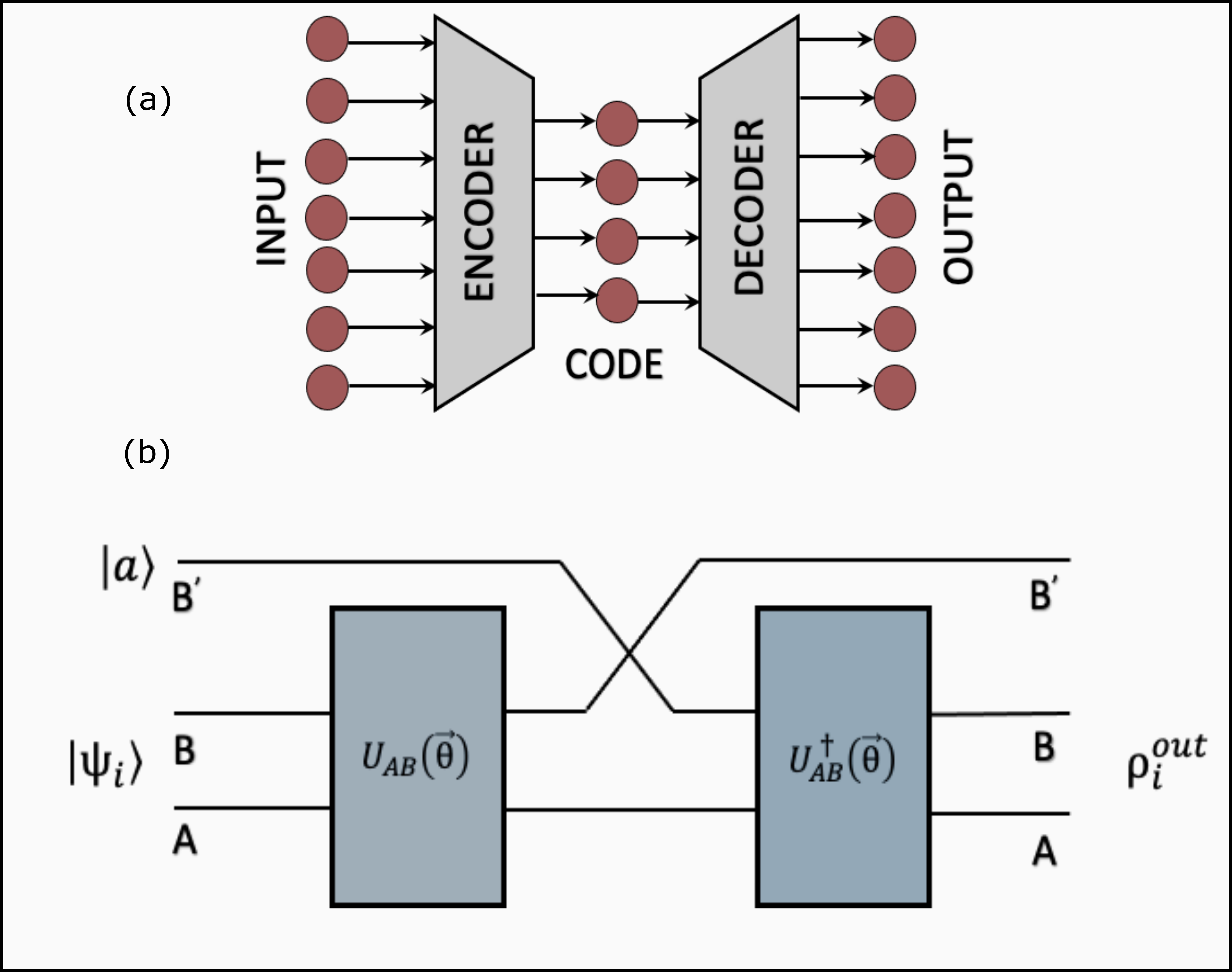
Like any other feed forward neural network it is trained through back-propagation to minimize the reconstruction error defined over it. For the simplest one layer encoder decoder circuit, with weights, biases and element wise activation function and , we can construct the norm loss function as follows,
| (78) |
where is the size of the training data set. Using a standard gradient descent one can train the parameters of the circuit to minimize the loss output. A regularization term might be added to ensure that network isn’t overfitting to the training dataset. Here we described an undercomplete autoencoder that made use of no regularization term. Overfitting here is avoided by ensuring a small latent code size. Depending on the error function, inputs, and size of the latent space we can construct autoencoders that have different functionality. A sparse encoder for instance has the same latent space size as the input and minimizes the number of activations in the latent space, implemented by a -regularization term on the latent space. A denoising encoder, takes inputs that are overlayed with minimal perturbations to reconstruct the original image. A contractive autoencoder tries to ensure that samples that are close in the input space have a similar encoding representation.
3.3.4.1 Quantum enhanced variants
To generalize a classical encoder to the quantum setting we start with building a unitary circuit that allows information to be compressed into a smaller set of qubits with a garbage state in the remaining qubits that can be replaced with a reference state. We start with an ensemble of pure states , where is an qubit system, is a qubit system. Let be the encoding unitary that takes as input a pure state from the ensemble. The system in the output is then swapped with a reference state and we try reconstructing the input state with a decoder given by the unitary . The objective function to maximize is given by
| (79) |
where
| (80) |
Here , denotes the fidelity between the states, is a swap gate that swaps the corresponding qubits and represents the parameters of the unitary circuit that needs to be trained. It can be show that the perfect fidelity is obtained when the output state of the encoder circuit produces a product circuit, i.e, 242. Thus we could alternatively define the maximizing objective function as the fidelity over the trash system B with respect to the reference state as,
| (81) |
This problem can thus be framed within the context of developing unitary circuits that works to disentangle qubits. It has been shown that using circuits of exponential depth it is always possible to disentangle qubits 243. Other alternative implementation include using approximate quantum adders trained with genetic algorithms 244 and generalization of feed forward neural networks as quantum circuits to implement autoencoders 245
3.3.5 Variational Encoders
Unlike autoencoders that try and provide useful latent space representation, variational autoencoders (VAEs) are used to learn the distribution that models the latent space. The decoder thus generated can be used to sample the input space working similar to Generative Adversarial Networks (to be discussed shortly). They have found their use in unsupervised 246 and semi-supervised learning 247. Let be the conditional likelihood of the decoder and be the the approximated posterior distribution the the encoder computes, where is the input vector and is the latent vector. We train the network on the parameters , to reduce the reconstruction error on the input and have as close possible to . Thus we would like to minimize the following evidence lower bound loss function (ELBO),
| (82) | |||||
where is the expectation value with respect to the specified distribution and is the KL divergence between the distributions and x is input from the training set. The later equality of the above expression is obtained by expressing using Bayes theorem and regrouping terms. The KL divergence regularizes the expression allowing for continuity (neighbouring points in latent space are mapped to neighbouring points in input space) and completeness (points in latent space map to meaningful points in input space for any chosen distribution). At this point 2 assumptions are made to allow for training. Firstly, is a Gaussian distribution and is a multivariate Gaussian that can be re-expressed as to allow for gradient back-propagation (reparametrization trick) , where and is an element wise product.

3.3.5.1 Quantum enhanced variants
Khoshaman et al 249 developed a quantum variational autoencoder that makes use of a Quantum Boltzmann Machine (QBM) 250 to evaluate the gradient updates used in training. A QBM is an energy model defined as,
| (83) | |||
| (84) | |||
| (85) |
where , , are pauli operators and governs the distribution of the states . The ELBO is defined with a cross entropy term as follows,
| (86) | |||||
| (87) |
where in the second line we have used Golden Thompson-Inequality( ) to express the intractable first term with a lower bound. Similar to the classical case, a reparametrization trick is employed to effectively evaluate gradients and the trace is taken to be concentrated at the state . See 249 for reparametrization trick in the continuous and discrete case setting.
3.3.6 Generative Adversarial Network (GAN)
Generative adversarial network (GAN) was introduced by Ian Goodfellow et al in 2014 251 and is considered to be one of the major milestones of machine learning in the last 10 years. Its applications extends to art 252, science 253, video games 254, deepfakes and transfer learning 255. A GAN consists of generator and discriminator that are trained simultaneously to learn a given distribution by competing against each other. The goal of the generator is to generate fake samples that cannot be distinguished from the true samples of input data. The goal of the discriminator is to correctly distinguish the fake samples from true samples, thus solving a well understood classification problem. This game has a Nash equilibrium point that is attained when the generator is able to generate samples are distinguished with a probability of , making it no better than a random guess. Let the generator take a random input from a distribution (usually taken to be a gaussian distribution) to generate samples from the distribution . Let be the discriminator that takes inputs equally likely sampled from (true distribution) and to output the probability of data coming from . The objective function for the discriminator is thus given by,
| (88) |
where the first term is the error in determining the true samples to be fake and the second term is the error in determining the generated samples to be true. The generator on the other hand tries to maximize this loss function against the trained discriminator, i.e, the objective function of the generator is given by
| (89) |
The parameters of the generator and discriminator are trained alternatively till the discriminator no longer is able to differentiate from . Thus the distributions are equal in the eyes of the discriminator and we have managed to create a generative model for the given training samples. The discriminator is discarded after the training. can be thought of the distribution that represents the domain set of the problem and thus the generator works to extract features of the input vector. The trained generator can be further re-purposed for transfer learning on similar input data. A conditional extension referred to as cGAN (conditional GAN) allows for generating inputs from a specific class by imposing additional restrictions on the random input vector provided. This restriction can be thought of selecting from classes within the domain set. To train a cGAN the discriminator also needs to be provided with this additional label input to constrain classification within the chosen class.
3.3.6.1 Quantum enhanced variants
In the quantum generative adversarial network (QGAN) 256, we have a source that outputs true samples and a generator that outputs fake samples. Both and takes an input state , label and random noise to output a density matrix in the system qubits. The noise vector supports to provide a distribution for the generator on the output qubit state corresponding to a given input label. With equal probability we choose between and to create a density matrix that is fed into the discriminator. Alongside the sample output from or provided, the discriminator takes as input the label used to generate the state, a bath that works as scratchpad and an output qubit to measure the probability of the source of the sample. Figure 20 provides a sketch for the working of the QGAN. The objective function can thus be given by,
| (90) |
where is the state output by the source and is the state output by the generator and represents the measurement made at the output qubit of the discriminator. The first and second term in the trace comes from the discriminators success in correctly predicting states from source and generator respectively. The cost function has been derived using measurement probabilities to keep the expression linear, unlike the maximum likelihood optimization used for the classical case. Given the optimization function, gradients can be computed using parameter shift trick or re-expressing it as a sum of simple unitary operations 257. For a complete discussion on the derivation of cost function, analyzing limiting cases and computing gradients corresponding to the parameters, refer 248.
3.4 Tensor Networks

Tensor network states constitute an important set of variational quantum states for numerical studies of strongly correlated systems in physics and chemistry as they attempt to construct global quantum states from tensors associated with local degrees of freedom. 258, 259. Expressing a quantum many-body systems defined on qubits requires complex coefficients. Storing and manipulating these numbers of coefficients on a classical computer poses a big challenge while simulating strongly correlated systems. Luckily physically relevant quantum states often possess limited amount of entanglement wherein only a subset of these coefficients are necessary to describe these states efficiently. Tensor networks provide a natural language to model complex quantum systems (states and operators) on which amount of entanglement (or correlations in the case of mixed-state dynamics) is conveniently restricted. The representation is such that the complexity of the structure grows linearly with qubit but exponentially with the amount of entanglement in the system. It thereby allows manipulation of quantum states residing in large Hilbert spaces with polynomial amount of resources. The classical simulation of low entangled systems (whose entanglement grows at most polynomially with system size ) becomes tractable using Tensor Network algorithms like Density Matrix Renormalization Group (DMRG) [Discussed in detail in Section 3.4.5] and Time-Evolving Block Decimation (TEBD)260, 261.
Tensor Networks are graphic representation of tensors in Einstein notation such that a rank-n tensor is represented by a box with n indices projecting out of it. The connections between tensor signify the set of indices of tensors which are contracted. Hence the final rank of a tensor network is determined by number of free edges. A quantum state in n-dimensional Hilbert space is a basically a rank-n tensor and can be written as,
| (91) |
where represent that local basis states and the coefficients are the amplitude of wave function in a given basis state .
The idea to using Tensor Networks to represent quantum systems is motivated from the very famous Area Law262 which states that the ground state of the Hamiltonian resides in the low entangled space such that entanglement entropy between any two partitions of the system grows as the area of the surface separating them. The entangled entropy is usually quantified in terms of the von Neumann entropy of a quantum many-body systems which is defined as , where is the density matrix of the state. It serves as a befitting measure of the degree of quantum correlation that exists between any of the two-partitions of the system under consideration. Area Law has been proven only for gapped Hamiltonians in one-dimension by Hastings 263 and has been studied intensively for higher dimensions [See section IV of review 262 for detailed discussion on Area Law in higher dimension]. Area Law guarantees an efficient description of ground states by a Matrix Product State and justifies the Density-Matrix Renormalization Group algorithm. Each of these two methods will be discussed in detail in Section 3.4.1 and Section 3.4.5 respectively.
Tensor Networks can be broadly classified into two main groups: those based on matrix product states (MPS), tree tensor network state (TTN) and their higher dimensions analogues (ex. PEPS); and those based on the multiscale entanglement renormalization ansatz (MERA). We shall discuss applications of TN in Section 5.2 and in Section4 and Section 5.3
3.4.1 Matrix Product State (MPS)
A pure quantum state of a -qubit system can be described by the sum of tensor products of orthogonal states in two subsystems. The Schmidt decomposition 49 of with respect to the partition reads,
| (92) |
where and are the state of the subsystems A and B and ’s are the Schmidt coefficients of the quantum state with respect to the partition. The Schmidt rank is defined by the number of non-zero Schmidt coefficients. It is a natural measure of the entanglement between the qubits in A and B, popularly known as bond dimensions in the Tensor Networks community. The von-Neumann entropy between the two partitions is given by,
| (93) |
Sometimes entanglement entropy is measured in ebits where one ebit is the amount of entanglement possessed by a maximally entangled two-qubit Bell state. Now if the states and are further partitioned in a similar fashion such that in the end the states we are only left with small states defined on single qubits. Let these states be denoted by and the diagonal matrix containing Schmidt coefficient be denoted by . Then the quantum state reads as,
| (94) |
where are complex square matrices of order (the bond dimension). represent the state indices in the computational basis (physical indices). These format of representing quantum states is known as Matrix Product State.264 In the tensor network notation it can be described as [Fig. 21 (a)]. Operators can similarly be represented in Matrix Product form known as Matrix Product Operator (MPO).
Matrix Product States in theory can represent a Maximally Entangled state but the bond dimension at middle cut would grows as 264. For a MPS with fixed bond dimension , the quantum state residing in -qubit Hilbert space can now be represented using just parameters. Area Law limits the bond dimension of the ground state of local gapped Hamiltonians making them the best candidates for MPS representation. Evaluating inner products of two quantum states in MPS form takes
matrices in the Eq. 94 are usually absorbed into the nearby local tensor . The Matrix Product state is invariant of the contraction of the either to left or right. This gives MPS a gauge degree of freedom. Usually the gauge is fixed by choosing either one direction for multiplying giving rise to the left and right canonical forms of MPS. The process is known as canonicalization 265, 264. There is another kind of canonical form known as the Mixed canonical form 266 which is obtained by combining each to the left (right) of a given special site to its left (right) neighbouring .
3.4.2 Tree Tensor Networks (TTN)
Tree Tensor Networks provide another approach to model quantum states by arranging the local tensors in a tree-like pattern (See Fig 21(b)). A TTN can be formed from a -qubit quantum state using the Tree-Tucker Decomposition 267, 268. Like other tensor networks, TTNs are used as ansatz to simulate ground state of local Hamiltonian. 269, 270, 271 Tensors in TTN form the nodes of the tree which are connected to each other through bond indices. The physical indices appear on the leaf nodes. On contracting the bond indices, the TTN has free indices which represent the physical degree of freedom of the state. TTNs are a generalization of MPS and can in principle be non-binary as well 272, 273. A MPS can be thought of as a flattened TTN such that each parent node has one successor (bond indices of MPS) and another leaf node (physical indices of MPS).
The structure of TTN is inspired from spatial Renormalization Group. 274 At every layer of TTN, a coarse-graining is carried out between neighbouring sub-trees. Unlike MPS, the local tensors with access to physical indices in TTN are not connected directly to each other, the correlation between qubits is represented through the layers. The local correlation information is stored in the lower layers while the upper layers store long-range correlation information.
Each node in a TTN is three-dimensional tensors (except the root/uppermost node) with at most one upper index and two lower index and . The tensors can be written as . The space required to store a TTN grows as (See Theorem 4.1 267), where is the number of physical indices and is the bond dimension of local tensors. Each tensor in TTN is an isometry satisfying the following condition:
| (95) |
Choosing isometric tensor as in Eq.95 is advantageous in numerous ways. It simplifies the optimization of TTN and calculation of expectation values of local observables and it is also known to provide numerical stability to TTN algorithms.275. TTN can very well be generalized to higher dimensions by appropriately placing isometries across local physical indices and hierarchically merging sub-trees through more isometries. Tagliacozzo et al. 275 in their works demonstrate simulation of the Transverse-field Ising model on square lattice using a two-dimensional TTN. Their approach takes advantage of the Area Law which reduces their simulation cost to instead of .
Tree Tensor Networks form the basis of the multi-layer multi-configuration time-dependent Hartree (ML-MCTDH) methods which are used to perform quantum molecular dynamics simulations. In the report 276 authors compute the vibrational eigenstates of acetonitrile using TTNs. ML-MCTDH methods are a generalization of MCTDH methods which can be optimized using MPS as shown in the report 277.Authors make use of the DMRG algorithm to efficiently evaluate the mean-field operators represented in MPS format. The runtime of MCTDH methods scales exponentially with system size, hence the multi-layered MCTDH is used which makes use of Tucker decomposition to reduce the dimensionality of the problem and enables it to simulate larger systems.
3.4.3 Projected Entangled Pair States (PEPS)
PEPS is a generalization of MPS in higher dimensions or for arbitrary graphs.264 It get its name from the way it is constructed. Let a vertex of a graph contain edges, each edge can be represented by a virtual spin of dimension (bond dimension). The edges are described by a maximally entangled state . Now the vertex can be defined by a -rank tensor containing entangled states. Ultimately this tensor is projected onto the physical spin through a linear map, , where d is the local dimension of the physical state.
In one dimension (k=2), an entangled pair of states are projected onto the physical index. While in a square lattice, each local tensor has at most four neighbours. [See Fig 21. (d)] Hence the local tensor can be written as , where the is the physical index and , , , and are bond indices. Hence storing a PEPS requires space, where is the number of qubits along a side of the square, is the dimension of the physical local state and is the bond dimension. Performing computations on PEPS is difficult,278 for instance evaluating the inner products of PEPS scales exponentially with the . This is because any partition which divides PEPS into two equal parts always cuts bonds, hence while evaluating the inner product one has to form a rank- tensor as an intermediate.
PEPS can theoretically represent any state due it’s generic structure given that its bond dimension can be arbitrarily large. Due to this universality, PEPS serve as variational ansatz in numerical simulation of a wide variety of quantum systems. It can easily prepare physically important states like GHZ and Cluster State 279 using . With D=3, PEPS can prepare a Resonance Valence Bond states. 280 Kitaev’s Toric code which finds its applications in quantum error correction and demonstrates non-trivial topological properties can be prepared using PEPS with D=2. 281 It is widely known that PEPS can efficiently approximate ground states of gapped local Hamiltonian which satisfy the area law. In the report 282 author show that they can compute the expectation values of local observables in quasi-polynomial time. Jordan propose algorithms to compute the ground states and time evolution of two-dimensional Hamiltonians defined on infinite-size lattice using PEPS. 283 It is known that it is difficult to simulate systems with long-range correlations on PEPS, but Gu et al. extensively studied these systems to demonstrate the power and versatility of PEPS. 284 They studied both systems which exhibit symmetry breaking phase transition (transverse field Ising model) and those that show topological phase transition ( gauge model, Double-semion model).
While PEPS have been designed to study quantum systems on classical computers, there have been approaches to simulate them on a quantum computer for faster computations. Schwarz et al. in their report 285 presented an algorithm to prepare a PEPS on a quantum computer which scale only polynomially with the spectral gap and the minimum condition number of the PEPS projectors. In the consecutive year they came up with another algorithm to prepare topologically projected entangled pair states on a quantum computer with similar runtime. 286 Specifically they simulated the resonance valence bond state which is hypothesized to contain topological spin liquid phase.
3.4.4 Multi-scale Entanglement Renormalisation Ansatz (MERA)
MERA 288 is a powerful class of Tensor Networks which can be used to study gapless ground states and properties of systems near criticality. Despite its huge success in representing a wide variety of states, MPS is scalable only for gapped systems with exponentially decaying correlations and the Area Law is strictly satisfied. Owing to its hierarchical structure, MERA allow long-range correlations and shows a polynomially decaying correlations [Shown in Eq. 5 of Ref 289]. The entanglement entropy of a -qubit 1D gapless system grow as and hence they can be naturally represented by a MERA.
The architecture of MERA is inspired from the Renormalization Group. 265, 290 Its structure is very similar to TTN with an additional type of tensors known as disentanglers () [shown in Fig. 21. (c) using blue circles]. These are unitary tensors satisfying,
| (96) |
whereas the isometries () [depicted using red triangles in Fig. 21. (c)] satisfies Eq. 95. To recover a TTN from MERA one can simply replace the disentangler with an Identity tensor.
Entanglement in MERA builds up due its layered structure. To dissect a sub-system of -qubits from the system requires at least bonds to be broken. Hence the maximum entanglement entropy generated by the MERA goes as . That is why MERA allows logarithmic divergence from the Area Law. 265, 289
Storing a MERA on a classical computer requires space polynomial in number of qubits and the bond dimension. Performing computations using MERA is simplified due to it structure. It can perform efficient computation of local expectation values and correlators by only contracting over the shadow (causal cone) of the local operator, i.e, the tensor which are directly connected to the operator and those tensors on higher levels which are further connected to these tensors. The isometries and disentanglers which lie outside this shadow contract themselves with their conjugates to give unity.
3.4.5 Density Matrix Renormalization Group (DMRG)
DMRG is one of the most successful algorithm for simulation of condensed matter systems. It was introduced by White 291 in the pre-Tensor Network era. The algorithm has changed a lot over the years and has been simplified by adapting to the language of tensor networks. In the following discussion, we will be describing the modern DMRG algorithm using Matrix Product State formulation. 266
Finding the ground state of a Hamiltonian is challenging problem and yet is one of core problem in physics, chemistry, and material sciences. Even for one-dimensional k-local Hamiltonian it is known to be QMA-complete 292 i.e. it’s difficult to solve it in polynomial time even with access to fully functional quantum computer.
Since the ground state of a gapped local Hamiltonian is known to reside in low entanglement regime by the Area Law. DMRG algorithm makes use of this property to find the solution of the local Hamiltonian problem. The algorithm makes use of an ansatz which succinctly represents the state with bounded entanglement (Matrix Product State). The ground state of the Hamiltonian is attained by minimizing the energy of the system,
| (97) |
Before starting the algorithm the Hamiltonian has to be converted into a Matrix Product Operator so that it is compatible with MPS. Since its a k-local Hamiltonians which can be written as, , where are local hermitian operators acting on at most k-qubits. Each can be converted into a MPO defined on k physical indices using recursive Singular Valued Decomposition as explained in Section 3.4.1. Once local operators are converted to MPO, they can be added using MPO addition operation, which is basically a direct sum operation over the bond indices. (See section 5.2 in Ref. 266 for details)
The initial MPS can be created using random tensors of desired dimension. At each step of DMRG a contiguous set of sites are chosen which is to be optimized and is designated as the system. While everything outside the system is called the environment which is kept fixed. By performing local optimization over the system states iteratively, the ground state of the given Hamiltonian is attained. Usually it requires several sweeps over the complete lattice to reach convergence which depend on the complexity of the Hamiltonian and also the choice of the initial state.
To perform local optimization over system, the environment qubits are contracted to form a reduced Hamiltonian () whose energy is then minimized.
| (98) |
Energy minimization of can be analogously performed by solving the following eigenvalue problem,
The system state so obtained updates the current system state. The system can be defined by any number of qubits. For single qubit systems the bond dimension remains fixed while working with two or more site system can allow the bond dimensions to be changed dynamically. Basically, the local optimization procedure for multi-site system returns the state defined on multiple qubits. This state has to decomposed into a MPS using recursive Singular Value Decomposition before replacing them at the current state. Since SVD gives us the complete set of singular values we can choose to trim the bond dimensions which are below the threshold of the accuracy required. Usually larger system size means more accurate results and the trial state converges to the ground state in lesser number number of sweeps. But it also increase the overall computation cost. The computational cost heavily depends on the local optimization procedure which can be improved by using iterative algorithms like Lanczos which only computes smallest set of eigenvalues and eigenvector of a given operator. Since we are only interested in the ground state of reduced Hamiltonian, Lanczos algorithm can massively cut down the computation cost.
3.4.6 Quantum enhanced Tensor Networks
There are numerous connections between tensor networks and quantum circuits. These relations lead to interest into two broad research directions. First one is the classical simulation of quantum circuits using Tensor Network. There are works demonstrating implementation of quantum algorithms like Grover’s algorithm and Shor’s algorithm in Matrix Product State (MPS) 293, 294 and Tree Tensor Network (TTN) framework 295. Recently a report showed classical simulation of the random quantum circuit using Tensor Network.296 The same circuit which was implemented on the Sycamore quantum processor to demonstrate "Quantum Supremacy" by Google.297 There has been massive improvement over the years in the runtimes for evaluating Tensor Network classically. In a recent report by Huang et al. 298, they demonstrated a new method called Index Slicing which can accelerate the simulation of random quantum circuits through tensor network contraction process by up to five orders of magnitude using parallelization. Markov et al. 299 theorized the time complexity of simulating quantum circuits using Tensor Network. A quantum circuit with a treewidth (a measure of how far a graph is from being a tree) and gates can be deterministically simulated in time. Another research direction which has been gaining traction due to advents of noisy intermediate scale quantum (NISQ) computers is the optimization of Tensor Networks using quantum computers. 300, 301. There are Quantum Machine Learning models which uses ansatz inspired from Tensor Network. 215, 302 The analogy between TN and quantum circuits can be exploited to develop an efficient state preparation mechanism on a quantum computer. There have been efforts in creating quantum states in MPS303, TTN302, PEPS285, and MERA304 format using quantum circuits.
Since the dimensions of the associated tensor grow exponentially with the depth of the quantum circuit associated with it, it is possible to prepare certain tensor networks with large bond dimension on a quantum computer that cannot be efficiently simulated on a classical computer. These states are of utmost importance because there is a definite quantum advantage associated with them. Authors in the report 304 demonstrated preparation of such a state called Deep-MERA which can be represented by a local quantum circuit of depth consisting of two-qubit gates. The expectation values of local observables of a DMERA can be computed in time on a quantum computer while a classical computer would take time, where is the desired precision and L is the number of qubits.
Schwarz et al. 285 demonstrate a procedure to efficiently prepare PEPS on a quantum computer that scales polynomially with the inverse of the spectral gap of Hamiltonian. There also have been efforts to use the advantages of Tensor Networks and Quantum Circuit simultaneously by fusing them. In the report 305, authors introduced a hybrid tree tensor network architecture to perform quantum simulation of spin lattice Hamiltonian with short-range interactions. They simulated two-dimensional spin systems as large as qubits which require operations acting on at most 9 qubits. Their method can be generalized to arbitrary trees to represent qubit system, where and are the maximal depth and degree of the tree. It would require circuits for computation and the cost for measuring local expectation values would be , where is the bond dimension of the TTN. They provide an efficient representation of a quantum state whose elements can be evaluated on a near-term quantum devices. When compared against standard DMRG on MPS and imaginary-TEBD on PEPS, they produce results more accurate by up to two orders.
4 Case for Quantum computing enhanced Machine Learning
4.1 Universal function approximation through supervised learning on a quantum computer
In this section, we shall specifically highlight some of the recent claims that propose a theoretical guarantee for supervised machine learning tasks on a quantum computer, with these claims being the successful mimicking of arbitrary unknown functional dependence with high accuracy. It is thus needless to say that the benefits of these claims if realized can enhance the learning capabilities of supervised models for both quantum and classical data even beyond the precincts of physical sciences.
Several significant proposals have been reported recently that attempts to approximate a function (say ) using a quantum circuit where are classical data entries. Intuitively this can be framed as a supervised learning task where one has access to a dataset which is assumed to follow the functional inter-relationship . The crux of the problem is therefore to learn a hypothesis which closely mimics the actual function within a certain error tolerance. To perform such tasks on a quantum computer and learn the hypothesis one needs to encode classical data onto a quantum state first. Mitarai 306 proposed a data-uploading scheme on a quantum circuit for such a scenario. The scheme maps with wherein one requires access to th power for each datum with into an qubit state as . The tensor product structure of the many-qubit state creates non-linear cross terms of the kind . Following this data-encoding, the state can be acted upon by any parameterized unitary (say ). This will be followed by a measurement protocol using a pre-defined operator (say ) to learn the hypothesis function . The hypothesis function is optimized with respect to the parameters using an appropriate loss function until the desired tolerance is reached i.e. at where The authors claim that the encoding above is capable of approximating a larger class of functions than what classical supervised learning tasks can achieve. To substantiate this claim the authors argue that if classical processors could mimic every kind of function, which can be realized from such quantum data-encoding, then that would mean the classical device in principle learn the input-output relationship of complex computational models like quantum cellular automata 307 which is known to not being achievable using polynomial resources on a classical device. Numerical experiments for fitting the time evolution of transverse Ising model and a binary classification task of a non-linearly separable data were performed with the above encoding with great success.
Perez-Salinas 308 demonstrated how to construct single-qubit classfiers using efficient data-reuploading which is essentially sequential loading of classical data entries. Many powerful insights into the function learning ability of a quantum circuit through data-encoders has been recently elaborated in Ref 309. The work explicates if the data-encoding unitary is expressed as and repetitions of such unitaries in the circuit are made along with parameterized unitaries (say as above) for training the model then the frequency components of the hypothesis function when resolved in the Fourier basis are entirely controlled by the encoding Hamiltonian family . However, the Fourier coefficients are influenced by the remaining part of the circuit i.e. the trainable unitaries as well as the measurement operator . The authors further show that repeating the encoding in parallel or in a sequence would lead to a similar frequency spectrum. Under the assumption that the trainable part of the circuit is general enough to realize any arbitrary unitary, then it is possible to choose encoding Hamiltonians that can generate any arbitrary frequency range asymptotically. Using this fact the authors prove that it is possible for the hypothesis function learnt by such a quantum circuit to mimic any square integrable function within an arbitrarily preset tolerance. This thereby lends to universal expressibility to such hypothesis functions. The importance of this result is many-fold as it allows one to not only realize that expressive power of the family of functions learnt from supervised learning task on a quantum circuit is extremely high but also allows one to design unitaries, set number of necessary repetitions etc to augment the learning process. Universality in discriminative learning wherein a hybrid quantum model to learn the parameters of an unknown unitary was used, have also been illustrated recently 310. Other than these expressive capacity of parameterized quantum circuits have been thoroughly investigated recently 311. Since most of NISQ era quantum ML models are indeed variational, much of the insight from these studies are directly transferable.
4.2 Power of Kernel estimation and data-classification from Quantum computers.
In this section we shall highlight some of the key results that has been demonstrated in recent years regarding the superiority of constructing kernel matrix elements from the quantum computer as opposed to a classical processor. Such kernel estimates are necessary for a variety of supervised learning algorithms like Kernel-Ridge Regression (see Section 3.2.2) or for classification tasks like in Support-Vector Machine or SVM (see Section 3.2.7) to name a few. Kernel-Ridge Regression on a classical processor has been extensively used in chemistry for estimating density functionals 312, simulating non-adiabatic dynamics across potential energy surfaces 45, dissipative quantum dynamics 128 and even procuring molecular and atomic properties like atomization energies 313, 314. We shall return to a subset of these applications and explore them in detail in Section 5.3. Even for classification, kernelized variants of SVM on a classical processor have been useful for demarcating phases of matter, or for delineating malignant tumors from non-malignant ones 315 which would be of use to biochemists and oncologists. We shall return to a subset of these applications in Section 5.2. Thus the learning capabilities of all the aforementioned algorithms can be augmented if quantum computing-enhanced kernel estimates are used. Kernelized SVM has also been used extensively for drug-designing process , in drug-induced toxicity classification 316 etc. We shall discuss some of these in Section 5.5. In fact a study has already demonstrated quantum advantage recently 317 wherein kernel SVM on an actual quantum device () was used with classical processing to delineate active vs inactive drug candidates for several diseases. The authors note faster training time on a quantum processor than on the classical processor for larger dataset sizes. We shall discuss this specific example in detail in Section 5.5.4.
It must be emphasized that for classification tasks, apart from quantum Kernel methods, the quantum instance-based learning algorithms could also outperform classical learners. Estimating the distance between the test data and the training ones is always crucial in the instance-based learning algorithms. For instance, in the nearest neighbor algorithm, one of the most typical instance-based learning frameworks, the label of the test data is determined by the nearest training data. In 2013, Lloyd and coworkers proposed a quantum clustering algorithm for unsupervised QML156, showing that estimating distances and inner products between post-processed vectors in N-dimensional vector spaces then takes time on a quantum computer. On the contrast, sampling and estimating distances and inner products between post-processed vectors on a classical computer is exponentially hard157.The significant speedup yields considerable power of the quantum instance-based learning algorithms as well. In fact a specific example of this class of algorithms which inherits the aforesaid advantage has also been recently designed by one of the authors 318 and applied for phase classification of material which will be of importance to material scientists. More details on such examples can be found in Sec.(5.2) and will not be elaborated herein. Here we shall specifically discuss the advantages of estimating the kernel on a quantum processors that has been noted recently for certain tasks which thereby promises exciting opportunities for kernelized quantum supervised learning with applications in physics and chemistry.
- 1.
Quantum-enhanced feature maps and kernels were defined in Section 3.2.1. As mentioned therein, Ref 117 provides two strategies for efficiently performing kernel-based machine learning algorithms using a quantum computer. The first is an implicit approach wherein the kernel matrix is estimated through an inner product once a quantum circuit for state preparation with encoding classical data is in place. With access to the entries of the kernel-matrix from the quantum computer, the actual ML algorithm is then performed classically. The other approach is the explicit approach, where the full ML task is performed on the quantum computer itself. Ref 117 adopts the first approach by encoding each entry of a given feature vector in the phase information of a multi-mode squeezed state and shows the corresponding kernel obtained through inner product of such states is expressive enough for classification tasks. To exemplify the second approach, it also used the two-mode squeezed state as a data-encoder and then applied a variational circuit (say ) followed by photon-number measurement and assigned the probability of a binary classification task to obtain two specific Fock states in the two-modes. Using the distribution obtained from the QC, the authors could linearly separate a dataset with 100 % accuracy. However, the authors note that the primary data-encoding strategy adopted in the paper is through the preparation of squeezed states in continuous variable quantum computing which can be efficiently simulated classically 319, 320. They further mention that inclusion of non-Gaussian elements like cubic-phase gates 97, non-linearity in photon-number measurements321, classically intractable continuous-variable instantaneous quantum computing or CV-IQP circuits 322 may lead to non-trivial kernel estimation task wherein the power of quantum computers can be better used. Similar results as these are also reported in Ref 318 wherein classical data was not-only encoded within the phase information of a multi-mode squeezed state but also in the amplitude. Proper comparisons of such squeezed state encoded kernels with Gaussian kernels were also investigated using standard datasets from scikit learn 323.
- 2.
The first work to exemplify an advantage is Ref 324. The algorithm in Ref 324 performs a standard support-vector machine classification task (discussed in Section 3.2.7) with (training feature vectors for input), and (testing feature vectors). The labels where the set . The algorithm only had access to the training labels () and its job was to evaluate an approximation to the testing labels i.e obtain which matches with with high probability. Unlike in the previous reference, the data-encoding feature map used did not produce product states. The specific data-encoding unitary used is the following:
(99) where is the number of qubits, denotes the nature of the unitary i.e if the unitary is local. For simulations the work used . Ref 324 argued that the above mentioned data-encoding is hard to simulate classically. The feature vector size i.e and the feature maps are defining the unitaries in Eq.99 are
(100) The first classification protocol which the authors in Ref 324 implemented is the explicit approach wherein after the above-mentioned data-encoding a variational circuit (say ) was also implemented followed by a measurement protocol. If the probability for certain specific bit-strings were higher than a tunable threshold, the algorithm was said to yield (or -1 otherwise). Numerical experiments were conducted on a 5-qubit superconducting circuit and the depth of the variational circuit was varied from 0-4. The training set had 20 data points for each label and so did the testing set. The success ratio as seen in Fig 3 of Ref 324 was close to 100% for 4 layers of the variational circuit. In the second part of the numerical experiment, the authors followed the implicit scheme in which only the estimates of the kernel matrix were obtained from the quantum computer. The rest of the classification task was performed classically once that was done. The constructed kernel matrix from the actual hardware agreed fairly well with the ideal one (see Fig. 4 in Ref 324) and classification task using it was of 100 % accuracy. After this demonstration of a data-encoding scheme which is hard to simulate classically, several other numerical experiments have been initiated to validate kernelized SVM on a quantum computer in different platforms 325, 326.
- 3.
A recent report 327 using the same feature-space encoding scheme as in Ref 324 above establishes that quantum enhanced kernels perform better for complex data classification tasks like geometric data patterns distributed according to Mersenne Twister distribution 328. Classical methods cannot achieve similar accuracy. However, if the data distribution is simple such that large differences exist between data that belongs to the separating classes then classical kernels would perform as well. Also, the study claims that simpler data encoding circuits for computing entries of quantum kernels may be less effective for certain data-classification tasks. Another study 329 has actually systematically studied the effect of noise and finite measurement samples and concluded that high noise content may expectedly be detrimental to the estimation of kernel entries on the quantum computer. However, the report 329 also proposes to mitigate the effect of the noise by classical pre-processing of the estimated noisy kernel like discarding the negative eigenvalues.
- 4.
A clear and most decisive exhibition of the power of kernelized variant of support-vector machine on a quantum computer for a classification task was highlighted in Ref 180. The motivation for the work was to demonstrate a specific example wherein estimation of the kernel Gram matrix on a classical processor would not only be not efficient, but the classification task itself would be provably disadvantageous. Also, the quantum advantage would be retained even in presence of finite sampling errors. The classification task chosen was based on the famous discrete-logarithm problem. The problem entails finding where with being a large prime number and being the generator of the multiplicative cyclic group . By generator one means an element such that for every element , one can write . In such a case is said to be the discrete-logarithm to base of in and is denoted by . It is believed that no classical algorithm can compute the discrete-logarithm in time which is polynomial in even though quantum algorithms like Shor’s algorithm is known to do it 53. The classifier function makes the following decision
(101) This classifier thus divides the set into two equal halves by mapping each of the halves to . The authors prove that a classical learning algorithm for this task cannot achieve an accuracy more than indicating that the best classical algorithm can only do random guessing for unseen test data. For the kernelized quantum SVM, however the authors propose the following quantum feature map/state
(102) where , for being some constant 180. The state-preparation circuit which prepares the above state is shown to be efficient using Shor’s algorithm 53. Using the above state-preparation strategy, the authors can estimate the kernel matrix for each entry in the training set as . Using this kernel, the authors rely on the usual SVM algorithm on a classical processor to construct a separating hyperplane and optimize the parameters for it. Once the parameters for the hyperplane are determined, classification of new test data also requires kernel matrix elements when new kernel estimates from the QC are invoked again. The authors call this procedure support vector machine with quantum kernel estimation (SVM-QKE) indicating that the quantum computer is only involved in constructing the entries of the kernel. The authors prove that SVM-QKE yields a classifier that can segregate the data in testing and training set with an accuracy of 0.99 in polynomial time and with a probability of at least over even random training samples. They further show that even when the QKE entries have a small additive perturbation due to finite sampling, the separating hyperplane so obtained is close to the exact one with high probability and so is the accuracy of the corresponding classifier. Since the kernel estimates from a classical processor cannot provably do better than random guessing, this classification task clearly explicates the superiority of quantum feature maps. Since then, several interesting demonstrations of kernel estimates on the quantum computer have emerged like using a linear combination of multiple quantum enhanced kernels with a variational circuit to enhance accuracy and expressivity over and beyond a single kernel for complex datasets 330, a fidelity based quantum kernel estimate between the members of the training dataset and the testing samples 331 or even distinguishing the classical data entries directly after mapping to quantum states in the quantum feature space using metrics with shallow circuit depth in a process which the authors call quantum metric learning 332 . Like in the above cases, numerical experiments have also been reported on real devices like a 17-qubit classification task 333 performed on Google’s Sycamore to segregate data in a 67-dimensional space with appropriate noise-mitigation strategies.
4.3 Power of Quantum-Neural Networks
In this section we shall highlight some of the recent reports wherein superiority of quantum computing enhanced neural network models have been demonstrated or theoretically proven in terms of its generalizability and expressive power, training capacity, resource and parameter requirements to mention a few. Neural networks in a classical processor have become the standard go-to method for many applications in chemistry and physics like in efficient state-preparation protocols using generative adversarial networks (see Section 3.3.6) 334, 335. Networks like CNN (see Section 3.3.2) have been used for the classification of phases of matter 336, 337, in quantum state-tomography, 338 and in structure and ligand based drug-designing protocols 339. Deep neural networks (see Section 3.3) have been also used for predicting molecular properties even with non-bonding interactions 340, in drug-induced toxicity detection 341, many-body structure of correlated quantum matter like molecules and materials, 342, 343 and even in molecular dynamics 344, 345. Generative models like Restricted Boltzmann Machine based neural-network representation of many-body quantum states 346 has been used for classification and understanding ground and excited state properties of quantum systems. We shall return to a subset of these applications in Section 5.1, 5.2 5.3, 5.4 and 5.5. It is thus apparent that all the aforesaid algorithms stand to benefit from any quantum advantage seen in the development of neural network based models on a quantum processor. In fact, in certain cases, direct advantages have already been reported. For example, the authors have reported a quantum circuit-based implementation of a Restricted Boltzmann Machine based ansatz for any of the electronic states of molecules and materials347 which requires polynomial resources for its construction. Similarly for quantum version of CNN which has been used for classification of phases in the Ising model 215, the authors claim a more parameter reduction. We shall return to these applications and their description in Section 5.2 and 5.3. Herein we enlist some of the recent examples wherein quantum superiority has been seen or theoretically conjectured thereby promising many novel applications in chemistry and physics which can be realized in future. More theoretical insight into the learning mechanisms and generalizability of quantum computing enhanced neural networks are discussed in detail in Section 6.4.
- 1.
Quantum-neural networks (QNN) have been discussed in Section 3.3. Each such network has three generic components - a data encoding circuit (often called feature map) which accepts classical data as input and usually encodes them into the amplitudes of a quantum state (Other encoding schemes are also possible. See ref 116) followed by a layer of parameterized unitaries. Finally, measurement protocol is exercised whose outcome is post-processed on a classical computer to minimize a loss function and alter the parameters of the last layer of unitaries variationally until the desired convergence is reached. A recent report has suggested that such networks can be more expressive and faster trainable than corresponding classical networks if the data encoding circuit possesses non-trivial entangling gates which can identify hidden correlation among data entries 348. The work used an input data-set and a parameter vector . The input distribution is the prior distribution and is the output distribution from the QNN given the input and specific parameter set. Using this they constructed the empirical Fisher information matrix ( 349 as follows:
(103) where denotes the sample size. The authors found that the eigenvalues of the Fisher information matrix for 100 samples with in the case of the QNN were fairly uniformly distributed contrary to that in the classical neural network wherein eigenvalues were largely concentrated near zero indicating the relative flatness of the optimization surface and difficulty in trainablity of the model with gradient-based schemes 350. They used an ‘easy-quantum’ model as well with data-encoding scheme without any entangling gates and found the Fisher information spectrum to be within the two limiting cases of a classical NN and a full quantum NN. The results are retained for .The authors in Ref 348 thereafter promised a metric for effective dimension defined below as
(104) where is the number of data samples, is the normalized Fisher information matrix and is the volume in parameter space and . The physical motivation of defining an effective dimension is to quantify the expressibility of the model i.e. estimate the size of the space all possible functions which the model class can successfully mimic with the Fisher information as the metric 351. Using the above definition of the effective dimension, the authors show that the full QNN has the highest effective dimension compared to the easy quantum model (without entangling gates in the circuit encoding the features) and even the classical neural network for and size of data (see Fig 3(a) in Ref 348). They also demonstrated that the full QNN trains faster and achieves lesser loss function values within smaller number of iterations compared to the other two (see Fig. 3(b) in Ref 348). The conclusion remains invariant to training even on the real hardware.
- 2.
Recently, a new report has been published 352 which extends the famous no-free lunch theorem 353, 354 to learning process in a quantum neural network (QNN) wherein the training data-set may be intrinsically entangled with a third accessible register. The no-free lunch theorem (NFL) for classical learning task is deduced for an unknown map , say where the size of the set is and that of set is . One generates a training set consisting of points from this function defined as . In general in the supervised learning setup, this set is used to construct a merit-function where is the hypothesis function that is expected to mimic the unknown function . The merit-function is minimized to obtain the parameters defining the hypothesis function which can then be used to make predictions for unseen . To quantify, how well the approximate function resembles the actual one one can define a risk function as follows:
(105) where is the prior probability distribution of sampling the input and is the probability that the output of the hypothesis function differs from the actual output for the specific input. The statement of NFL which the authors used is the following
(106) where the averaging of Eq. 105 has been done over many training sets and many different functional maps . The result in Eq.106 indicates that the average risk can be minimized if the number of training samples and hence is entirely determined by the training set independent of the specific details of the optimization scheme. In the quantum setting, the authors deduce a version of NFL wherein the data-set contains entries of quantum states that are entangled with an accessible auxillary quantum system. The setup of the deduction involves a unitary map both of which are -dimensional. The user herein has access to another auxillary quantum system (say ). The training set contains pairs of states which are entangled with as follows:
(107) All input states are entangled with the same Schmidt rank The learning task is to design an unitary such that and . The risk function in this case is defined as
(108) where and and (not necessarily within ) and and the measure is over the Haar measure of states. The averaging of the above risk function over all training sets and unitary maps as before yields
(109) The bound actually holds for each and hence averaging over is unnecessary. It is derived under the assumption that over the training samples the outcomes of and match perfectly. Implication of the above bound is that for , the bound vanishes and the average risk can be minimized only if where is the dimension of . This indicates that if the input states are product states with the quantum system characterized by then exponentially many training samples might be required in . This result was previously obtained in 355. However for that is not the case. Specifically, in the limiting case of , a single training example would suffice to saturate the lower bound on the average. For any in between one can easily see that the number of training samples can be set to be far fewer than . The authors show numerical experiments on Rigetti’s quantum processor for unitaries and demonstrate that the average risk can be minimized well below the classically accessible limit by controlling r which alters entanglement with the third quantum system . Similar results were obtained even in the simulator. The concrete proof of the theorem restores hope that the size of the training set can be small yet a quantum advantage can be retained as long as entanglement is used as a useful resource which is not possible classically. This result joins the group of other results wherein entanglement have served similar roles like in superdense coding 356, 357 or quantum teleportation 358, 359
- 3.
This example is different in spirit than the previous ones as it demonstrates how the quantum convolutional neural network (QCNN) 215 which is discussed in detail in Section 3.3.2 can lead to efficient parameter reduction compared to other methods of quantum phase classification. The power of a quantum classifier over and beyond that of a classical classifier has already been demonstrated for certain tasks in some of the points above. The task which the authors tested the QCNN was to segregate quantum states belonging to a particular phase given a training data-set where are the corresponding labels. The specific example was the symmetry-protected topological phase of a 1D spin-chain. The algorithm requires only parameters to classify such an -qubit quantum state which the authors claim is a two-fold exponential reduction in parameter space compared to other quantum classifiers. This essentially means that the QCNN is more expressive compared to other classifiers as it solves a relatively low-dimensional optimization problem without sacrificing the accuracy of the task at hand. Similarly, they also show that the sample complexity of QCNN which is defined as the number of copies of the input state that needs to be accessed by the algorithm for correctly identifying the phase, is lesser than from other techniques like direct evaluation of expectation values of certain operators which can also act as a marker of the phase. We shall return to this example in Section 5.2. Pesah 360 have demonstrated that in the conventional QCNN architecture there is absence of barren plateaus as the gradient estimates vanishes polynomially (and not exponentially) in the size of the system for random initialization . Recently MacCormack have extended the concept to introduce a variant of QCNN which is called the branching quantum convolutional network (bQCNN) 361. In QCNN as discussed in Section 3.3.2, the primary idea is reduction of the number of qubits while preserving important features. The convolutional layers perform multi-qubit unitaries for generating entanglement among the qubits whereas in pooling layers certain number of qubits are discarded through measurements and controlled rotations on nearby qubits are performed conditioned on the measurement results of the discarded qubits. The new reduced set of qubits is then fed into the convolutional unitaries again and the process is repeated. For bQCNN, the authors make a deviation at the pooling layer. Instead of using certain measurement outcomes only of the discarded qubits, the authors use all possible outcomes or binary bit combinations to design several different channels/branches for subsequent convolutional operation each of which is realized for a given bit string. This enhances the parameter requirement drastically as noted in the report. However the authors also demonstrate that the expressibility of the ansatz from bQCNN is higher than that of QCNN at similar circuit depth.
4.4 Power of Quantum Computers for Tensor-Network based Machine Learning tasks
In this section, we highlight an advantage that has been recently reported for a classification task performed using a tensor network ansatz on a quantum computer. Such classification can be extended to the physico-chemical domain like in ligand selectivity for structure-based drug designing (see Section 5.5.1) with the quantum benefit reaped. An example of another tensor network based classification of phases of a spin-model can be found in Section 5.2. Besides, Tensor networks on a classical processor have also been aggressively used for representing many-body states for a variety of applications like for spin-liquids 362, excitonic states in materials 363 and molecules 364. Quantum advantages as has been noted for the example below can be extended to such applications. We shall discuss such prospects with concrete examples in Section 5.3.2.
Recently, a report has illustrated the use of quantum architectures of Tree and Matrix Product state Tensor Networks 302 to demonstrate the working of a discriminative machine-learning model on MNIST dataset 365. The primary objective of the study was to perform classification and recognition of hand-written digits using a variational optimization procedure that can be efficiently carried out on a quantum hardware in the NISQ era. Classical data-entries (say ) from the data-set are mapped to a -qubit quantum state using the data-encoding protocol described below in Eq. 110
| (110) |
State is a product state which can easily be prepared by applying single qubit rotation gates on state. After state preparation, each set of qubits (say qubits where is the number of virtual states) is acted upon by a parameterized unitary gate. The scheme is inspired from coarse-graining techniques. After each parameterized unitary operation, qubits are discarded/reset and the other qubits proceed to the next step where they are merged with qubits coming from another set of qubits. This process is continued until the last 2V qubits remain which are acted upon by a unitary gate to produce output qubits. One or more output qubits are measured to determine the probability distribution of the output labels. While the model is agnostic to the grouping of the qubit sets, it is usually wise to group qubits that represent local regions in the input data. This ansatz is motivated from a Tree Tensor Network (see Fig. 22). The optimization problem which they solve involves classification of hand-written digits using a loss-function that penalizes the difference in the probability of attaining the true-label from the measurement protocol as opposed to the most-probable incorrect label. The algorithm used is adapted from Simultaneous Perturbation Stochastic Approximation (SPSA) 366 with momentum being included inside the gradient estimates 199. The accuracy of the method as reported is extremely high i.e. with the lowest percentage error being 87% and an average test accuracy of over 95%. The authors noted that for usual quantum algorithms, encoding such a -qubit state and applying tunable unitaries would require -physical qubits. However, the tree-structure in the ansatz with sequential measurements allows the authors to use physical qubits indicating that the scheme is qubit efficient. It must also be emphasized that merely using a tree-tensor network approach (TTN) on a classical processor would require a space complexity of 367 where is as defined before the number of virtual states. This result indicates that the TTN ansatz on the quantum computer is more expressive than a corresponding classical implementation as similar accuracies are afforded even with a reduced bond-dimension (bond-dimension is usually denoted by where and as seen here scales logarithmically for the quantum TTN version whereas would have a cubic scaling for classical TTN). The authors also perform a systematic analysis of the effect of noise on the algorithm and concluded that the degradation of the performance was only 0.004 with a strongly enhanced () noise parameters thereby indicating the resilience of the algorithm.

5 Applications
5.1 State preparation protocols and Quantum State Tomography
With the rapid advancement of quantum technology in the past decade, there is an increased demand for efficient methods that can verify the generated quantum states according to specific needs. This is primarily important for the validation and benchmarking of the quantum devices. To address this, quantum state tomography (QST) aims to obtain the statistical inference of the unknown quantum state of the system based on the information of the expectation values of a complete set of observables 49, 368, 369, 370, 371. However, the traditional approach to QST has been pushed to its limits for the large quantum platforms available today 372. This is because the number of measurements required for full reconstruction of the quantum state scales exponentially with the system size which poses a critical challenge for performing QST even for moderately sized systems. Also, in order to obtain valuable insight about the physical observables of the system and to estimate them accurately, the measurement outcomes need to be stored and processed for which exponential amounts of classical memory and computing power are required which makes the technique infeasible for practical applications.
Apart from the problem of exponential scaling for complex systems, another drawback for accurate estimation of a quantum state is the inherent noise in the present day noisy intermediate-scale quantum (NISQ) devices 84. Because of this the measurements available are of limited fidelity and in certain cases, some of the measurements are even not accessible. Several methods have been proposed as a means of an alternative approach to the traditional QST such as matrix product state tomography 371, neural network tomography 373, 374, 375, 376, quantum overlapping tomography 377, shadow tomography 378, 379. Because of the noisy nature of the quantum systems since not all measurements are available at high fidelity, there have also been approaches that try to carry out QST based on incomplete measurements 380, 381, 382 such as maximum likelihood estimation (MLE) 383, 384, 385, 386, 387, 388, Bayesian mean estimation (BME) 389, 390, 391, 392, and maximal entropy formalism based QST 393, 394.
Quantum detection and estimation theory has been a prominent field of research in quantum information theory since the 1970s 395, 396, 397 and the rapid progress in quantum communication and computation in the past two decades motivated the use of big data for the classification of quantum systems through quantum learning and quantum matching machines 398. The notion of self-improvement of the performances of quantum machines via quantum learning was introduced by Ron Chrisley in 1995 in 399 through the example of barrier/slit/plate feed-forward back-propagation network. In a feed-forward network, parameterized non-linear functions map an input state to an output state space. The interactions with the environment help the networks to modify those parameters such that each network can better approximate the resulting function. The proposed quantum implementation of such a network involved setting up a barrier with several slits in front of a particle beam. Some of the slits are designated as input slits and rest are the weight slits. Behind the barrier is a photo-sensitive plate on which the interference pattern is observed that serves as an output for each input slit configuration. Once an interference pattern of high resolution is obtained on the plate, the error, which is a function of the desired and actual output vectors, is calculated. The gradient descent method is applied by taking the partial derivative of the error function with respect to the control variables, the weights, and the slits are adjusted accordingly for the next reading so as to minimize the error function. After sufficient training, optimum values for the weight configuration are obtained that ensured minimal error on the training set. This feed-forward network established the correspondence between the neural networks and the quantum system and is one amongst the many diverse approaches for the practical implementation of quantum neural networks 400, 401.
One of the most valuable applications of quantum tomography is the validation and testing of near-term quantum devices called the NISQ devices. Leveraging the capabilities of quantum hardware of the gate-based NISQ devices, Alejandro et al in 402 proposed a hybrid quantum-classical framework called data-driven quantum circuit learning (DDQCL) algorithm for benchmarking and training shallow quantum circuits for generative modeling. Much like the various models encompassed within the Born machines 403, 404, 405, 406, the authors captured the correlations in the data set using the 2N amplitudes of wave function obtained from an N-qubit quantum circuit. However, the distinctive feature in their work is the use of quantum circuit as a model for the data set that naturally works as a Born machine, thereby avoiding the dependence on tensor networks for the same. They demonstrated their approach of training quantum circuits for preparation of the GHZ state and coherent thermal states thereby illustrating the power of Born machines for approximating Boltzmann machines.
Finding an effective quantum circuit that can optimally carry out a desired transformation between the input and output quantum states also constitutes an important aspect of QST. In 407 the authors proposed a machine learning based optimization algorithm for quantum state preparation and gate synthesis on photonic quantum computers. They used the continuous-variable quantum neural network architecture 408 as an ansatz whose optimization was carried out on the Strawberry Fields software platform for photonic quantum computation 409. Using the proposed method, the authors were able to achieve high fidelities of over 99 using short-depth circuits given only the target state as an input.
Another quantum state preparation method was presented in 410 based on reinforcement learning which is a machine learning training architecture framework that finds an optimal solution to a problem based on the principle of rewarding the desired actions and penalizing the negative actions. The authors made a comparative study of the performances of three reinforcement learning algorithms: tabular Q-learning (TQL), deep Q-learning (DQL), and policy gradient (PG), and two traditionally used non-machine-learning methods: stochastic gradient descent (SGD) and Krotov algorithms, demonstrating their efficiency with reference to quantum state preparations under certain control constraints. Their results illustrated the effectiveness of reinforcement learning algorithms in solving complex optimization problems as the algorithms, especially DQL and PG, performed better amongst the five algorithms considered for state preparation under different types of constraints.
Parameterized quantum circuits (PQC) are yet another machine learning model that utilizes the resources of both quantum and classical computation for applications in a variety of data-driven tasks. 411 presented a comprehensive review of various machine learning models involving PQC and also their applications in diverse fields including quantum tomography. Another class of algorithms within the domain of quantum machine learning is hybrid quantum-classical Variational Quantum Algorithms (VQAs) 412 that has been gaining popularity in the recent years with numerous applications 413, 414, 415, 416, 417, 418, 419. VQAs try to reduce the quantum resource allocation by using shallow quantum circuits for carrying out computations on a quantum device. One such algorithm was proposed in 420 by Wang et al to prepare quantum Gibbs state on near-term quantum hardware using parameterized quantum circuits. On such devices it is in general quite difficult to prepare Gibbs state at arbitrary low temperature just like finding the ground states of Hamiltonians 421. Preparation of quantum Gibbs state of a given Hamiltonian has its applications in a variety of fields like many-body physics, quantum simulations 422, quantum optimization 423, etc. In the method proposed by Wang et al minimization of free energy serves as the loss function. However, within the calculation of free energy estimation of entropy is the most challenging part 424. To tackle this problem they used truncation of Taylor series of the von Neumann entropy at order K and thus, the truncated free energy was set as the loss function whose minimum would correspond to the optimal parameters of the quantum circuit giving the Gibbs state. The estimation of the Taylor series expansion terms of entropy can be practically carried out using the well-known swap test 425, 426 and therefore, their method can be physically realized on a near-term quantum hardware. To validate the approach they numerically showed the preparation of high-fidelity Gibbs state for Ising chain and XY spin- chain models and were able to achieve fidelity of at least 95 for a range of temperature.
Another kind of quantum state preparation commonly termed as Quantum State Tomography relies on accessing experimentally measured observables. We shall discuss, hereby, how various techniques within the domain of machine learning/deep learning have been applied to perform QST.
As machine learning and neural networks became increasingly popular with its applications in many diverse fields, the concoction of quantum mechanics and machine learning algorithms also started surfacing 427, 428, 156, 177. The development of quantum annealing processors 429 deemed a natural fit for testing the machine learning algorithms on a quantum hardware 430, 431 to check for any quantum advantage. In the initial stages quantum mechanics was only used to facilitate the training for solving classical problems which, in fact for certain problems, did result in obtaining polynomial speed-ups relative to classical training methods 432. Although the training of the Boltzmann machines using quantum processors did result in accurate training at a lower cost, however, the success of machine learning algorithms based on classical Boltzmann distribution inspired the proposition of a quantum probabilistic model for machine learning called quantum Boltzmann machines (QBM) based on Boltzmann distribution for quantum Hamiltonian 433. In QBM, not only the training is performed utilizing the quantum nature of the processors but also the model in itself is inherently quantum. The data modeling and training of Boltzmann machine is carried out using the equilibrium thermal states of the transverse Ising type Hamiltonian.
However, the training procedure used in 433 suffered from two limitations: a) brute force techniques are required to find out the transverse field terms as it cannot be learned through classical data making it very hard to find the full Hamiltonian, b) quantum Monte Carlo methods can be used to efficiently simulate the transverse Ising models and therefore, using the training method with transverse Ising models in thermal equilibrium did not show a clear quantum advantage. In 434, the authors proposed the quantum analog of the generative training model that included quantum data sets in the training set so that their QBM is capable of learning the quantum terms along with the classical ones. The training of the Boltzmann machine to incorporate quantum data was carried out through two methods: POVM-based Golden-Thompson training and state-based relative entropy training (quantum equivalence of KL divergence). The relative entropy training method allowed the QBM to clone the quantum states within certain level of approximation and given considerable number of copies of the density operator for training of QBM, it could reproduce approximate copies of the input state. Thus, although different from the traditional quantum state tomography wherein an explicit representation of the state operator is available at the output, the generative training of the QBM resulted in a quantum process that can learn Hamiltonian models for complex quantum states which in itself is a form of partial tomography.
Machine learning techniques offer a big advantage of representing high dimensional data in compressed form which can be really favourable for QST which in itself is a highly data-driven technique. In 2018, Torlai and colleagues 373 utilized this property of the neural networks for obtaining the complete quantum mechanical description of highly entangled many-body quantum systems based on the availability of a limited set of experimental measurements. Their method involves training of a restricted Boltzmann machine (RBM) using simulated measurement data for the true state. Their RBM architecture comprises of a layer of visible neurons for encoding the measurement degrees of freedom and a hidden layer of binary neurons for encoding the tunable parameters. The training of the RBM is performed such that the the generated probability distribution resembles closely to the given data distribution and parameters are tuned depending on the desired degree of accuracy that is required for reconstruction. They demonstrated their approach by first benchmarking the neural network tomography of the N-qubit multipartite entangled W state. They also demonstrated QST for more complex systems consisting of quadratic spin Hamiltonians, namely the transverse-field Ising model and the XXZ spin-1/2 model.
According to the authors, their RBM model works really well for entangled many-body systems and quantum-optic states. However, when there is an unstructured data as in the case of states generated from random unitary operation, the performance of the RBM goes down. The paper also did not highlight some of the pertinent questions such as what should be the size of the training set, or the optimal number of hidden neurons, and the dominance of RBM over the other contemporary machine-learning approaches. Also, in the demonstration of their approach, both in the case of the tomographic reconstruction of the W state or ground states of the quadratic-spin Hamiltonians, the wavefunctions considered are real which decreases the measurement degrees of freedom required for state reconstruction and thereby, dramatically reduces the tomographic overhead.
Another neural network based quantum state estimation method empowered by machine learning techniques was presented in 435 in 2018 for full quantum state tomography. Instead of reducing the number of mean measurements required for full state reconstruction, the work focuses on speeding up the data processing in full QST without the assumption of any prior knowledge of the quantum state. Their training model is based on standard supervised learning techniques and the state estimation is carried out using a regression process wherein a parameterized function is applied for the mapping of the measurement data onto the estimated states. For a single state reconstruction, the computational complexity of their model is , where d is the dimension of the Hilbert space, and was the fastest amongst the full QST algorithms such as MLE, LRE, BME, etc. at the time.
A further application of neural network in the field of state tomography was presented in 376 where local measurements on reduced density matrices (RDMs)436, 437, 438, 439, 440 were used to characterize the quantum state. Using the recent approach of measuring RDMs and thereby reconstructing the full state is a convenient alternative to the traditional QST approaches as the whole system can be characterized in polynomial number of parameters as opposed to the exponential parameters required for full reconstruction in the traditional QST techniques. However, QST via local measurements on RDMs is a computationally hard problem 441. In this work, the authors addressed this problem using machine learning techniques by building a fully connected feedforward neural network, as shown in Figure 23, to demonstrate the full reconstruction of the states for up to 7-qubit in simulation and also reconstructed 4-qubit nuclear magnetic resonance (NMR) states in experiments. Their approach also had comparable fidelities with the MLE method but with the additional advantage in terms of speed up and better noise tolerance.

Another machine learning assisted quantum state estimation technique based on convolutional neural networks (CNN) (Basic theoretical framework discussed in Section 3.3.2) was presented in 338 in 2020 for reconstructing quantum states from a given set of coincidence measurements for both pure and mixed input states. Their approach involves feeding the noisy or incomplete set of simulated measurements to the CNN which then makes prediction of the -matrix based on the decomposition method discussed in 442. The predicted matrix, which is the output, is then inverted to give the final density matrix. In order to compare the fidelity of the reconstructed states, the authors also implemented the Stokes reconstruction method 442 and found a significant improvement in fidelity for not just noisy data sets but also when the projective measurements are incomplete and thereby, demonstrating the advantage of CNN over the typical reconstruction techniques.
As an alternative means of QST several methods have been proposed, such as MLE, BME, and least-squares (LS) inversion 443, for efficient reconstruction of the quantum state. Since measurements on many copies of the state are required for efficient reconstruction of the quantum state so in order to gain maximum information from the measurements on the next copy, the measurements are adjusted based on the already available information from the measurements made thus far. This method of reconstructing the quantum state through adaptive measurements is called adaptive quantum state tomography. One such approach was introduced in 444 where self-learning algorithm was used in combination with different optimization strategies such as random selection, maximization of average information gain, fidelity maximization for quantum state estimation. A generalization of self-learning algorithm was presented in 390 in the form of adaptive Bayesian quantum tomography (ABQT) with the aim to optimally design quantum tomographic experiments based on full Bayesian inference and Shannon information. Through their adaptive tomography strategy the authors were able to achieve significant reduction in the number of measurements required for full state reconstruction in case of two qubits pure states in comparison to Monte Carlo simulation of the qubit systems. The experimental realization of the ABQT method was also carried out in 445 for two qubit quantum system which did show a significant improvement in the accuracy of state estimation in comparison to the nonadaptive tomographic schemes. Recently, neural adaptive quantum state tomography (NAQT) was introduced in 446 that utilizes the neural network framework to replace the standard method of Bayes’ update in the ABQT scheme and thereby obtained orders of magnitude faster processing in estimating the quantum state while retaining the accuracy of the standard model. Basically, in the adaptive Bayesian-type tomography, the quantum space is discretized into samples and with each sample there is an associated weight that gets updated with each new measurement according to the Bayes’ rule in order to update the prior distribution to the posterior distribution of the quantum state space. However, with the increase in the number of measurements the likelihood function becomes sharply peaked with a tiny subset of the sample states having the majority weights. This can lead to a numerical singularity which is then avoided by resampling of the weights onto the space states which is computationally a very expensive process. In 446 the authors have used machine learning algorithm to map the Bayesian update rule on a neural network to replace the traditional approach and thereby eliminate the problem of resampling of the weights saving the computational cost significantly without compromising on the accuracy of the reconstruction process. In comparison to the ABQT technique, the NAQT approach was able to speed up the reconstruction process by a factor of a million for approximately measurements and is independent of the number of qubits involved and type of measurements used for estimating the quantum state.

In 2013, another useful method was proposed in 441 wherein linear regression estimation (LRE) model was used to identify optimal measurement sets to reconstruct the quantum state efficiently. The model was relatively straightforward where the authors converted the state estimation problem into a parameter estimation problem of a linear regression model and the LS method was employed to determine the unknown parameters. For a d-dimensional quantum state, the computational complexity of the method for state reconstruction is and thereby saves up the cost of computation in comparison with the MLE or BME method. A natural extension to this work, in terms of both theory and experiment, was presented in 448 in order to improve the tomography accuracy by better tomographic measurements via adaptive tomography protocol that does not necessarily require non-local measurements from experiments. The method is called recursively adaptive qauntum state tomography (RAQST) primarily because the parameters are updated using the recursive LRE proposed in 441 and using the already collected data the measurement strategy is adaptively optimized for obtaining the state estimation. The authors also performed two-qubit state tomography experiments and show the superiority of RAQST method over nonadaptive methods for qauntum states with high level of purity which is an important criterion for most forms of information processing methods.
Another significant machine learning approach is the Generative adversarial network (GAN) (Basic theoretical framework is discussed in Section 3.3.6) based QST 334, 335 that basically involves learning the map between the data and the quantum state unlike the RBM-based QST methods where the map yields a probability distribution. In the GAN method, two competing entities: generator G and discriminator D, engage with the objective to output a data distribution from some prior noisy distribution. Both G and D are parameterized non-linear functions consisting of multi-layered neural networks 251. With each step of optimization the generator becomes better at yielding outputs closer to the target data and the discriminator becomes better at detecting fake output. Inspired by the classical model, the quantum generative adversarial network (QGAN) was introduced in 449, 450 where quantum processors are used for running the neural nets of generator and discriminator as well as the data can be both quantum and classical. Thus, making the entire system quantum mechanical, at the end of the optimization process the generator can reproduce true ensemble of quantum states without the discriminator being able to distinguish between the true and generated ensemble.
The first proof-of-principle experimental demonstration of the QGAN algorithm was presented in 447 in a superconducting quantum circuit on datasets that are inherently quantum for both the input and the output. The QGAN algorithm employed was able to reproduce the statistics of the quantum data generated from a quantum channel simulator with high level of fidelity (98.8 on average). Their experimental approach involves a superconducting quantum circuit for the generator G that outputs an ensemble of quantum states with a probability distribution to mimic the quantum true data whereas the discriminator D is used to carry out projective measurements on the true and the generated data in order to distinguish the two based on the measurement outcomes. The optimization process based on the gradient descent method consists of the adversarial learning by the discriminator and the generator in alternative steps that is terminated when the a Nash equilibrium point is reached i.e. G produces the statistics such that D can no longer differentiate between the fake and the true data. The experimental protocol of the implementation of the QGAN algorithm is shown in Fig. 24.
In 451 the authors introduced conditional generative adversarial network (CGAN) based QST as in the standard GAN approach there is no control over the output as the generator input is random which can be addressed using CGAN. Because of the improved control over the output, the CGAN led to many diverse applications in a variety of fields 452, 453, 454, 455, 456. With the CGAN based QST the authors were able to achieve higher fidelity of reconstruction, faster convergence and also reduced the number the measurements required for reconstructing a quantum state as compared to the standard model of state reconstruction using MLE. Also, with sufficient training on simulated data their model can even reconstruct the quantum states in a single shot. In their CGAN approach, the measurement operators () and the measurement statistics are the conditioning input to the generator which then outputs a density matrix that is used to generate the measurement statistics by calculating tr(). These measurement statistics and the experimental measurement statistics serve as the input for the discriminator which then outputs a set of numbers to distinguish between the generated statistics and the true data.The standard gradient-based optimization techniques are then used to train the network which is completed when the discriminator is unable to differentiate between the generated statistics from the generator and the true data. With better control over the output the CGAN approach can further find its applications in efficiently eliminating noise from experimental data by training it on noisy simulated data as well as it can have potential advantages in adaptive tomography as well by improving on the choice of adaptive measurements for better reconstruction of quantum states.
The huge success of attention mechanism-based neural network generative model 228, 457, 458 to learn long-range correlations in natural language processing (NLP) 459 prompted for its applications in QST owing to the entanglement among qubits that can also be learnt through the self-attention mechanism used in the former case. The self-attention mechanism computes a representation of a sequence by relating different positions of a single sequence and has been very successful in a variety of sub-fields under NLP 460, 461. In 459 the authors proposed the first purely self-attention based transduction model, the Transformer, for deriving global dependencies between input and output without the use of recurrent neural network (RNN) or convolutions. Just like other transduction models, the Transformer also uses an architecture of fully connected layers for both the encoder and decoder 462, 228, 463 using stacked self-attention that results in significantly faster training than architectures based on recurrent or convolutional layers. To the best of our knowledge the quantum-enhanced version of the Transformer has not been studied yet. However, the application of Transformer on quantum data has shown tremendous potential, as discussed below in the context of QST, for future research in this field.
The long-range correlations exhibited by entangled quantum systems can be modeled analogous to the sentences in natural language using informationally complete positive operator-valued measurements (IC-POVM). Therefore, with this motivation, recently, Cha et al proposed the ’attention-based quantum tomography’ (AQT) 464 to reconstruct the mixed state density matrix of a noisy quantum system using the Transformer 459 architecture for the neural network. In this work they first benchmark their approach against previous neural network based QST using RNN 465 that demonstrated a high fidelity classical description of a noisy many-body quantum state. To compare the performance of AQT with other state-of-art tomographic techniques they considered Greenberger–Horne–Zeilinger (GHZ) state as their target state for upto 90 qubits and a built-in simulated error resulting in a mixed state. They showed that the complexity of learning the GHZ state can be improved by an order of magnitude when compared with the RNN method. They also benchmark AQT against MLE for a 3-qubit system and found a superior quantum fidelity of reconstruction for the AQT with the additional advantage of being scalable to larger systems. Furthermore, they were also able to reconstruct the density matrix of a 6-qubit GHZ state using AQT, with a quantum fidelity of 0.977, which is currently beyond the tomographic capabilities of IBM Qiskit.
QST becomes a formidable task as the size of the quantum system increases. In order to address the problem, in this section of the review, we presented research based on several machine learning driven QST techniques such as RBM based QST for highly entangled many-body quantum systems, characterizing quantum systems using local measurements on RDMs, using CNN for state reconstruction, adaptive QST through self-learning and optimization based algorithms, VQAs for QST, generative models like GANs and attention based QST. Although the use of classical machine learning algorithms and deep neural networks have proven to be very effective in finding patterns in data but for implementation on a quantum computer, loading classical data onto quantum devices can present a serious bottleneck for the implementation of these algorithms 466. Since large number of independent parameters are required for reconstructing the quantum state that scales exponentially with the system size and therefore, using quantum machine learning algorithms directly on the quantum states of the system can help in the learning and optimization of these parameters much more efficiently, owing to their ability of handling larger Hilbert space. As mentioned in the above sections, generative machine learning models such as quantum Boltzmann machine (QBM) and quantum generative adversarial network (QGAN) provide valuable insights into exploiting the full capabilities of the present day quantum computers in order to reproduce the desired quantum states. The improvement of quantum hardware with time also calls for their validation and benchmarking and QML can play a major role in the design of cost-effective quantum tomography techniques and protocols that can be easily implemented on the NISQ devices.
5.2 State classification protocols
Classification is always one of the most significant applications for classical machine learning(ML) or quantum machine learning(QML). Due to the fact that people are prone to make mistakes when establishing connections among various features, ML and QML are often able to improve the efficiency dealing with the classification problems. Each instance in the dataset used by machine learning algorithms should be represented with the same set of features, which could be continuous, categorical or binary161. The learning process is then denoted as supervised machine learning if all instances are given with known labels. Generally, the classification problems can be divided as binary classification and multi-label classification. Binary classification is a classification with two possible outcomes. For example, classify if an atom or molecule is excited or at ground state. Multi-label classification is a classification task with more than two possible outcomes. For example, classify the electrical resistivity and conductivity of materials as conductor, insulator, semiconductor or superconductor. We shall focus extensively on the supervised QML assisted classification problems in chemical systems, specifically, where the output of instances admits only discrete un-ordered values and then discuss unsupervised learning strategies too.
The process161, 467 of applying supervised ML or QML to a typical classification problem with physico-chemical is demonstrated in Fig.(25). The first step is to collect the dataset from chemical experiments. Due to the very existence of errors in measurement and impurities in reaction, in most cases the raw dataset contains noise and missing feature values, and therefore significant pre-processing is required468. The second step is to select appropriate algorithms and initialize the classifier model. Then, split the dataset using cross-validation and feed the classifier model with training data. Next, predict the label for test dataset, and evaluate error rate of the classifier model. Additionally, parameter tuning should be repeated until an acceptable evaluation with the test set is obtained.
Classifiers based on decision trees (see Section 3.2.5) play important roles in various chemical problems, such as the toxicity prediction469, mutagenesis analysis470, and reaction prediction471. Even though, quantum decision trees are hardly applied independently dealing with intricate chemical classification problems, since simplicity, one of the key advantages of decision tree, could be eclipsed during the complicated mapping and learning process in QML.
Decision trees are sometimes applied along with other algorithms to analyze and demonstrate the key features of intricate classification process. Recently, Heinen and coworkers studied two competing reactive processes mainly with a reactant-to-barrier (R2B) machine learning model472, where decision tree generated by the R2B method systematically extracts the information hidden in the data and the model. Fig.(26) is a scheme of the tree generated from the R2B method. Blue dotted lines refer to an accepted change meaning only compounds containing this substituents at the position are considered. Orange dotted lines refer to substitution declined, meaning all compounds except the decision are kept. Vertical lines on the right of energy levels denote the minimum first (lower limit), and the third (upper limit) quartile of a box plot over the energy range. Numbers above energy levels correspond to the number of compounds left after the decision. Lewis structures resemble the final decision.

In the recent years there arise more than a few reports where Bayesian networks (BN) (see Section 3.2.6) based methods are applied solving various chemical classification problems. The BN approach shows fruitful capability in the predictions of chemical shifts in NMR crystallography473, simulation of the entropy driven phase transitions474, and particularly, the simulation of quantum molecular dynamics simulation475.
Quantum instance-based learning algorithms like k-NN (see Section 3.2.4) are also applied in chemical classification problems. Recently, the authors have studied the phase transition of based on a quantum instance-based learning algorithms318. The training instances are firstly assigned into several sublabels via the quantum clustering algorithm, based on which a quantum circuit is constructed for classification. Fig.(27) is a scheme of the quantum circuit implementing classification process of the quantum clustering algorithm. For training instances that are clustered into N sublabels, qubits are required representing the sublabels in the classifier circuit. Meanwhile, qubits are required to represent the test instance, where is denoted as the dimension of instance. For simplicity, here we assume that there are only 5 sublabels totally, and all instances are 2-d vectors. Thus, represent the possible sublabels and represents the test instance, meanwhile is operation corresponding to the centroid or mean value of the training instances under the same sublabel. Here Hadamard gates are applied on , preparing a uniform distribution of the possible sublabels. To improve the accuracy, the weighting scheme can be included by assigning as some certain quantum states corresponding to the weights.
For training instances that are clustered into N sublabels, qubits are required representing the sublabels in the classifier circuit. Meanwhile, qubits are required to represent the test instance, where is denoted as the dimension of instance. For simplicity, here we assume that there are only 5 sublabels totally, and all instances are 2-d vectors. Thus, represent the possible sublabels and represents the test instance, meanwhile is operation corresponding to the centroid or mean value of the training instances under the same sublabel. Figure is reproduced from Ref318. (Under Creative Commons Attribution 4.0 International License)
The process of classification of metallic and insulating states of are shown in Fig.(28). Fig.(28(a)) demonstrates the original data used for classification. All training instances are 2-d vectors (pressure and temperature), while the label is denoted by color. Red dots represent metallic state, and blue ones represent insulating state. Phase transition line indicated by the black solid curve. The sublabels left after quantum clustering algorithm is shown in Fig.(28(b)), where each sphere represents a sublabel, with center corresponding to the centroid or mean-value, and radius corresponding to the number of instances. Prediction of test instances are shown in Fig.(28(c)). Test instances in the blue part will be recognized with label ’insulating’, and label of test instances in yellow part will be predicted as ’metallic’.

Fig.(28(a)) demonstrates the original data used for classification. All training instances are 2-d vectors (pressure and temperature), while the label is denoted by color. Red dots represent metallic state, and blue ones represent insulating state. Phase transition line indicated by the black solid curve. The sublabels left after quantum clustering algorithm is shown in Fig.(28(b)), where each sphere represents a sublabel, with center corresponding to the centroid or meanvalue, and radius corresponding to the number of instances. Prediction of test instances are shown in Fig.(28(c)). Test instances in the blue part will be recognized with label ’insulating’, and label of test instances in yellow part will be predicted as ’metallic’. Figure is reproduced from Ref318 (Under Creative Commons Attribution 4.0 International License).
The quantum SVM (see Section 3.2.7) has also been applied into various classification problems, such as handwritten character recognition176, solar irradiation prediction476, and even the study of particle decays in high energy physics477. Additionally, in experiments provable quantum advantage has been demonstrated by the recent quantum classifiers based on a variational quantum classifier and a quantum kernel estimator—build on noisy intermediate-scale (NISQ) devices324. Though there are only a few attempts to deal with specific chemical problems with quantum SVM methods, quantum SVM demonstrate great capacity in classification problems, while the optimization process of quantum SVM leads to exponential speedup comparing with the classical version. Therefore, there exists enormous potential for the quantum SVM methods to assist chemical classification and regression problems.
It is always one of the most crucial challenge in the study of many-body problems that the dimensionality of the Hilbert space grows exponentially with system size, which leads tremendous difficulty to solve the Shrödinger equations. Among the modern numerical techniques designed to study the complicated systems, neural networks (NN) attracts enormous attention due to the remarkable abilities to extract features and classify or characterize complex sets of data. Modern ANN architectures, especially the feed-forward neural networks (see Section 3.3.1) and convolutional neural networks (see Section 3.3.2) have been playing significant roles in the classification problems of various fields. It is reported that the neural network technologies can be used to discriminate phase transitions in correlated many-body systems336, to probe the localization in many-body systems478, and even to classify the entangled states from separated ones337.
On the other hand, dramatic success of classical neural networks as well provokes interest developing the quantum version. More than 20 years ago, pioneers attempted to build up quantum neural networks(QNN), particularly, the quantum version of feed-forward neural networks479 (see Section 3.3.1). There were also reports where the QNN were applied into real classification problems, such as the vehicle classification480. The rapid development of hardware further provided more possibilities designing the QNN models.
Special-purpose quantum information processors such as quantum annealers and programmable photonic circuits are suitable fundamental implementation of deep quantum learning networks55, 481. Researchers also developed recurrent quantum neural networks (RQNN) (see Section 3.3.3) that can characterize a nonstationary stochastic signals482, 483. Additionally, there are some other QNN models aiming to supervised learning, such as the classifiers based on QNN and measurements of entanglement484. Even though, most of these models are actually hybrid models, as the activation functions are calculated classically, and the dataset are generally classical data.
In 2018 Farhi and Neven proposed a specific framework for building QNN that can be used to do supervised learning both on classical and quantum data485. For binary classification problems, the input instance can be represented by quantum state , where is a -bit binary string carrying information of the inputs, and an auxiliary qubit is set as initially. Totally there are qubits, qubits representing the input instance, and 1 qubit representing the label. After the unitary operation , the auxiliary qubit is measured by a Pauli operator, denoted as , and the measurement result or indicates the prediction of label. With multiple copies, the average of the observed outcomes can be written as . Further, we can estimate the loss function
| (111) |
where is the label of instance , which might be or . For a training set , the training process is to find the optimal parameters minimizing the loss function . However, in the numerical simulations, they did not find any cases where the QNN could show speedup over classical competitors for supervised learning485.
Meanwhile in 2018, researchers from Xanadu investigated the relationship between feature maps, kernel methods and quantum computing179. There contains two main steps in the classification steps. They attempted to encode the inputs in a quantum state as a nonlinear feature map that maps data to quantum Hilbert space. Inner products of quantum states in the quantum Hilbert space can be used to evaluate a kernel function. Then a variational quantum circuit is trained as an explicit classifier in feature space to learn a decision boundary. In the model, a vector from the input space is mapped into the feature space which is the infinite-dimensional space of the quantum system. The model circuit then implements a linear model in feature space and reduces the “infinite hidden layer” to two outputs. Though linear transformations are natural for quantum theory, nonlinearities are difficult to design in the quantum circuits. Therefore the feature map approach offers an elegant solution. Classical machine learning took many years from the original inception until the construction of a general framework for supervised learning. Therefore, towards the general implementation much efforts might be required as we are still at the exploratory stage in the design of quantum neural networks.
In 2019, Adhikary and coworkers proposed a quantum classifier using a quantum feature space486, with both quantum variational algorithm and hybrid quantum-classical algorithm for training. The input are encoded into a multi-level system, therefore the required number of training parameters is significantly less than the classical ones. Simulation based on four benchmark datasets (CANCER, SONAR, IRIS and IRIS2) shows that the quantum classifier could lead to a better performance with respect to some classical machine learning classifiers. In 2020, Wiebe’s group proposed circuit-centric quantum classifier487, which is a class of variational circuits designed for supervised machine learning. The quantum classifier contains relatively few trainable parameters, and constructed by only a small number of one- and two-qubit quantum gates, as entanglement among the qubits plays a crucial role capturing patterns in the data. The optimal parameters are obtained via a hybrid gradient descent method. The circuit-centric quantum classifier shows significant model size reduction comparing the classical predictive models487.
The impressive success of these hybrid methods provide an alternative to study the chemistry classification problems. There are plenty of attempts to study the phase diagrams classification with classical machine learning methods488, 489. It would be of great interest to study these problems with quantum or hybrid classifiers.
Recently 490 a report has proposed a variational quantum algorithm to classify phases of matter using a tensor network ansatz. The algorithm has been exemplified on XXZ model and transverse field Ising model. The classification circuit is composed of two parts: The first part prepares the approximate ground state of the system using Variational Quantum Eigensolver and feeds the state to the second part which is a quantum classifier which is used to label the phase of the state. Since the quantum state is fed directly into the classification circuit from the variational quantum eigensolver, it bypasses the data reading overhead which slows down many applications of quantum-enhanced machine learning. For both the parts, the quantum state is represented using a shallow tensor network which makes the algorithms realizable on NISQ devices. The first part of the algorithm represents the Hamiltonian matrix of the system in terms of Pauli strings and variationally minimize the average energy to prepare the ground state. A checkerboard tensor network scheme with tunable number of layers is used for the representation. For an -qubit state, the ansatz requires independent parameters, where is the number of layers in the circuit. In this scheme, maximally entangled state would require layers with periodic boundary conditions and for a critical one-dimensional systems is enough. This can be contrasted with a UCCSD ansatz which requires typically parameters 491 thereby necessitating a higher dimensional optimization. As mentioned before, the second part of the circuit i.e. the classifier receives the state from VQE part and applies a unitary . The unitary is again approximated using the Checkerboard tensor network ansatz. Then the output of the circuit is measured in Z-basis to determine the phase of the state using majority voting. For the transverse field Ising model the report demonstrated a accuracy with 4-layered classifier and for the XXZ model it was accuracy with a 6-layered classifier.
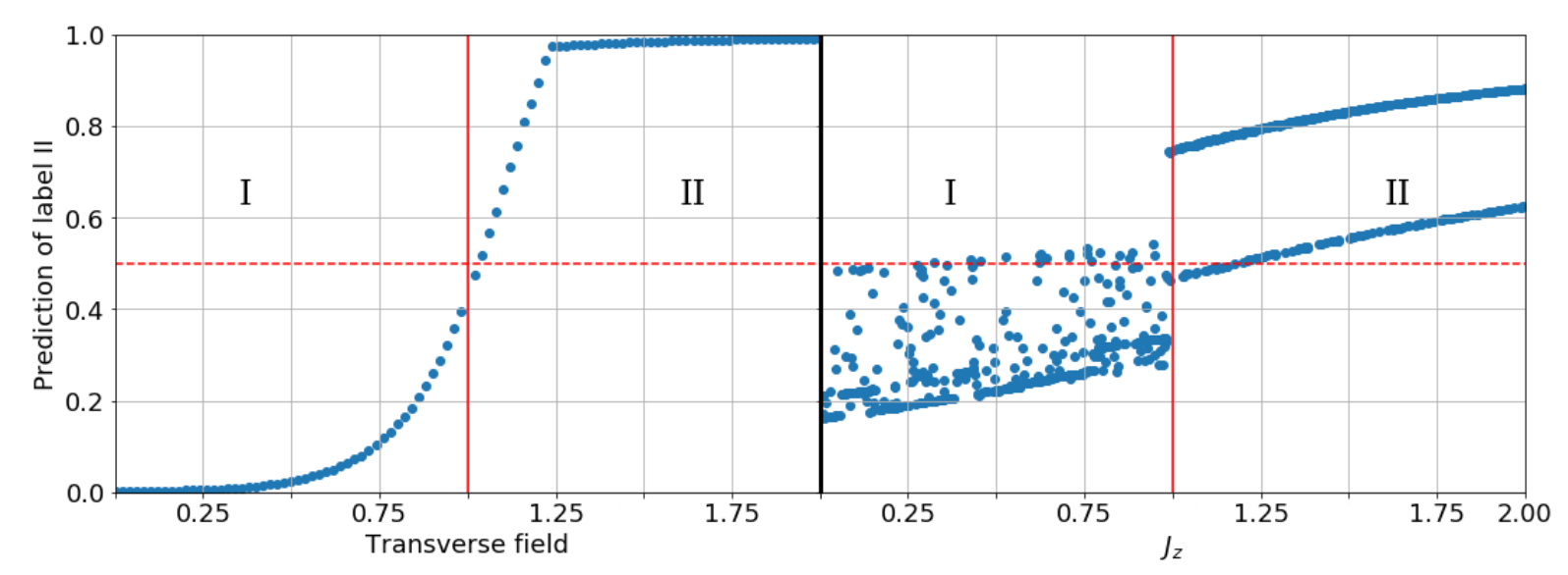
Picking up an appropriate algorithm is always crucial dealing with the classification problems The classifier’s evaluation is often based on prediction accuracy. Here we present three techniques estimating a classifier’s accuracy161. One popular technique is to split the training instances into two groups, where two-thirds are regard as training data and the other third is regard as test data. Another technique is known as cross-validation. The training set is manually divided into exclusive and equal-sized subsets in initial. Then for each subset the classifier is trained on all the other subsets. Thus, estimation of the error rate of the classifier is obtained by calculating the average of the error rate of each subset. The last one is denoted as Leave-one-out validation, which is a special case of cross validation. In Leave-one-out validation there is only a single instance in each subset. If the prediction accuracy can not reach the demand, another supervised learning algorithm should be selected, as shown in Fig.(25).
Additionally, we will present some remarks about the techniques as follows. Even though the optimal solution always depends on the task at hand, these remarks can prevent the practitioners from selecting a wholly inappropriate algorithm. Logic-based systems often perform better when dealing with discrete features. Decision trees are in general resistant to noise because of their pruning strategies. In contrast, most decision tree algorithms cannot perform well when diagonal partitioning is required. Interference allows a class of quantum decision trees to be penetrated exponentially faster by quantum evolution than by a classical random walk. Even though, these examples could also be solved in polynomial time by different classical algorithms164. BN methods are able to achieve its maximum prediction accuracy with a relatively a small dataset. Besides, BN methods train very quickly since they require only a single pass on the data either to collect the frequencies or to compute the normal probability density functions. The graph structure of BN can efficiently construct a quantum state representing the intended classical distribution, and a square-root speedup time can be obtained per sample by implementing a quantum version of rejection sampling173. Lazy learning methods require zero training time due the training instance is initially stored. On the other hand, k-NN is quite sensitive to the irrelevant features, and is generally intolerant of noise. Quantum nearest neighbor algorithm and quantum nearest centroid algorithm both show significant speedup comparing the classical version. In certain cases, there are exponential or even super-exponential reductions over the classical analog56. SVM methods generally perform better when dealing with classification problems with multi-dimensions and continuous features. Moreover, SVMs are still able to perform well when there exists a nonlinear relationship between the input and output features. Even though, a large sample size is required to achieve its maximum prediction accuracy. Optimization of quantum SVM is implemented by the quantum algorithm solving linear equations, leading to exponential speedup comparing to the classical version177.
Let us now focus on unsupervised approaches to classification briefly. The learning process is denoted as unsupervised when the given training instances are not assigned with the desired labels. Due to the absence of supervision, the unsupervised learning can hardly be applied to distinguish various types of chemicals or detect some certain structures. Instead, unsupervised learning process can find out the boundaries that divides the instances, so that it could be beneficial in the recognition of phase transitions. For instance, unsupervised machine learning methods can be applied to identify the phase transition to non-trivial many-body phases such as superfluids492, or to detect the topological quantum phase transitions493.
One important approach in the unsupervised QML is clustering methods. The clustering methods can be assigned as instance-based learning algorithms. Consider the k-means problem of assigning given vectors to k clusters minimizing the average distance to the centroid of the cluster. The standard unsupervised learning method is Lloyd’s algorithm, which contains the following steps494, 495: (1)Pick up the initial centroid randomly; (2)Assign each vector to the cluster with the closest mean; (3)Recalculate the centroids of the clusters; (4)Repeat steps (1-2) until a stationary assignment is attained. Based on the classical version, in 2013 Lloyd and coworkers proposed the quantum unsupervised machine learning method156, rephrasing the the k-means problem as a quadratic programming problem which is amenable to solution by the quantum adiabatic algorithm. In 2018, Iordanis and coworkers proposed q-means, a new quantum algorithm for clustering problem, which provides substantial savings compared to the classical k-means algorithm. In 2017, researchers implemented a hybrid quantum algorithm for clustering on a 19-qubit quantum computer496, which shows robustness to realistic noise.
Inspired by the success of neural network-based machine learning, Iris and coworkers proposed the quantum convolutional neural networks (QCNN) in 2019215 (see Section 3.3.2). A paradigm is presented where the QCNN is applied to 1-D quantum phase recognition. There are less applications of unsupervised QML compared to supervised learning in chemical classification problems reported so far. Even though, the recent advancements suggest the future that unsupervised QML could take a place in the study of complex many-body systems, especially in the recognition of phases.
5.3 Many-body structure and property prediction for molecules, materials, and lattice models and spin-systems
5.3.1 Machine learning techniques on a classical processor
Obtaining an electronic structure description for material systems has been a problem with continued research in Chemistry and material science. Since this task is a many-body problem, solving it with high accuracy is crucial as numerous material properties and chemical reactions entails quantum many-body effects. For a significant duration, performing electronic structure calculations were done using the Density Functional Theory (DFT), which is based on the effective single-particle Kohn-Sham equations 497. In DFT, the ground state energy of a many-electron system is written as a functional of the electron density, thereby reducing the many-body problem for an N particle wavefunction to just one. This has yielded accurate results with efficient computations compared to its predecessors, but the functional form of the exact solution is unknown and efficient approximations are made for practical purposes. Attempts have been therefore made to obtain such density-functionals using ML algorithms. One of the earliest study is due to Snyder 312 which constructed the kinetic energy functional for spinless fermions in a 1D box subjected to an external potential made from the linear combination of several gaussians defined on a dense spatial grid. Many such randomly selected external potentials were chosen as the training set with the actual labelled density and kinetic energy obtained by solving the Schroedinger equation as the training data. Thereafter kernel-ridge regression was used to construct the kinetic energy functional from the aforesaid known density with excellent accuracy. The oscillations in functional derivative of the so constructed kinetic energy functional were dampened by using the principal components. From the knowledge of this functional derivative a protocol to procure a self-consistent density field that minimizes the energy was presented. Since then many report exists which have attempted to construct density functionals especially the exchange-correlation functional 498, 499, 500, 501, 502, 503, 504, 505.
Kernel-ridge regression (see Section 3.2.2) has been extensively used in chemistry for a variety of other purposes too like predicting the energy of the highest occupied molecular orbital from three different molecular datasets 506 using two different technique to encode structural information about the molecule or for the prediction of atomization energies 313, 507 through a Coulomb matrix representation of the molecule wherein the energy is expressed as a sum of weighted gaussian functions. Recently many new schemes to represent structural features have also been designed 508, 314 wherein information about the environment of each constituent atom is encoded within its -body interaction elements each of which is a weighted sum of several gaussian functions. The distance metric between each such interaction representation between element and is considered to be the usual Euclidean norm. Atomization energies, energies for even non-bonded interaction like in water clusters predicted using such representations are extremely accurate314. More such examples can be found in topical reviews like in Ref 509. Caetano et al. 342 used Artificial Neural Networks (ANNs) (Theoretical framework discussed in section. 3.3) trained using the Genetic Algorithm (GA) to solve the Kohn-Sham equations for He and Li atoms. They used a network comprising of one neuron in the input layer, one hidden layer with eight neurons, and two neurons in the output layer. For the GA based optimization, the number of individuals N in the population was kept to 50. By generating the initial orbitals randomly and building the electron density, an effective Hamiltonian is constructed. The ANN is trained using GA to find the orbitals that minimize the energy functional and then the total energy is calculated, which is repeated until a convergence point. The results from the ANN were shown to be in good agreement with the other numerical procedures.
Performing higher order calculations like CCSD provides accurate results but have very high computational cost. While, methods such as semi-empirical theory PM7, Hartree-Fock (HF), or (DFT) provide less accurate results but scale efficiently. The work by Ramakrishnan et al. 510 corrects the lower-order methods to provide accurate calculations by training their model to to learn enthalpies, free energies, entropies, and electron correlation energies from a dataset consisting of organic molecules. The property of interest was corrected by expressing:
| (112) |
where, are regression coefficients, obtained through kernel ridge regression (Theoretical framework discussed in section. 3.2.8), , with being a hyperparameter that is tuned, is the Manhattan norm 511 measuring the similarity between the features of target molecule and molecule in the data .
Burak Himmetoglu 512 constructed a dataset incorporated from PubChem comprising of the electronic structures of 16,242 molecules composed of CHNOPS atoms. Having constructed the Coulomb matrices as in 511 defined by:
| (113) |
where, the atomic numbers are denoted by , and is their corresponding positions. Design matrices using the eigenvalues of the Coulomb matrices are constructed and two types of ML approaches are used to predict the molecular ground state energies. Firstly, boosted regression trees (Theoretical framework discussed in section. 3.2.5) and then ANNs are used, and their performances are compared.
Geometry optimization is a crucial task, which directly impacts the electronic structure calculations. The total energy calculations can prove to be quite expensive depending on the choice of electronic structure method. Hence, the number of evaluations of the potential energy surface has to be reduced considerably. A novel gradient-based geometry optimizer was developed by Denzel and Kästner 513, that exploits Gaussian Process Regression or GPR (Theoretical framework discussed in section. 3.2.8) to find the minimum structures. By comparing Matérn kernel with the squared exponential kernel, the authors show that the performance is better when Matérn kernel is used. The performance of their optimizer was tested on a set of 25 test cases along with a higher dimensional molybdenum system, molybdenum amidato bisalkyl alkylidyne complex, and was shown that GPR based approach can handle the optimization quite well.
In the work by Carleo and Troyer 346, it was shown that by representing the many-body wavefunction in terms of ANNs, the quantum many-body problem can be solved. They used this idea to solve for the ground states and describe the time evolution of the quantum spin models, viz. transverse field Ising, and anti-ferromagnetic Heisenberg models. Expanding the quantum many-body state in the basis :
| (114) |
where, is the wavefunction represented in terms of a Restricted Boltzmann Machine (RBM), which is the ANN architecture that was used in this study (Fig. 30 a). The description of Neural-Network Quantum States (NQS) results in the wavefunction to be written as , where denotes the tunable parameters of the neural network. The quantum states can now be expressed as:
| (115) |
where, the values of & {+1,-1}, & are the bias parameters corresponding to the visible and hidden layer respectively, and is the weight associated with the connections between & (see Fig. 30 (a)). For a given Hamiltonian, the average energy written as a statistical expectation value over distribution is computed. For a specific set of parameters, samples from the distribution are taken via Markov Chain Monte Carlo (MCMC) and the gradients of the expectation value are calculated. With the gradients known, the parameters are optimized in order to model the ground states of the Hamiltonian. The accuracy of the results were extremely high in comparison to the exact values. Recently Choo 514 have also extended the method to model ground states of molecular hamiltonians. The protocol maps the molecular hamiltonian onto the basis of Pauli strings using any of the fermion-qubit mapping like Jordan-Wigner or Bravi-Kitaev encoding that is routinely employed in quantum computing 515. Thereafter the wave-function as described in Eq. 115 is used to variationally minimized the ground state energy by drawing samples using Variational Monte Carlo (VMC) 514. Several insightful features like the fact that support of the probability distribution in the space of spin configurations is peaked over certain dominant configurations only near the Hartree-Fock state, out-performance of RBM ansatz over more traditional quantum chemistry methods like CCSD(T) and Jastrow ansatz, the efficacy of the various fermion-qubit mapping techniques in classical quantum chemistry simnulations etc were elucidated.
This NQS approach was then extended by Saito 516 to compute the ground states of the Bose-Hubbard model. Here, the quantum state is expanded by the Fock states. one-dimensional optical lattice with 11 sites and 9 particles, and a two-dimensional lattice with 99 sites and 25 particles were studied. The optimization scheme is similar to that in 346 and the ground states were calculated for the 1D and 2D cases were shown to be in good agreement with those obtained from exact diagonalization and Gutzwiller approximation respectively.
.
In the work by Coe 520, NNs were used to select important configurations in the Configuration Interaction (CI) method. By using just a single hidden layer, with binary occupations of the spin orbitals in the desired configurations, the transformed co-efficient of the configuration that fitted to the co-efficients in the training set, are predicted. The important configurations of stretched and at its equilibrium geometry were shown to have accurate predictions. This work was extended in their follow-up paper 521, in which the potential energy curves for , , and, were computed with near-full CI accuracy.
Custódio et al. 522 developed a feedforward neural network (Theoretical framework discussed in section. 3.3) to obtain a functional form for calculations pertaining to inhomogeneous systems within DFT and Local Spin Density Approximation (LSDA) framework. The network consists of an input layer with 3 neurons, a hidden layer with 20 neurons, and an output layer consisting of one neuron. The network was trained on 20,891 numerically exact Lieb-Wu results for 1000 epochs. The authors test their network on non-magnetic and magnetic systems and through their results claim that the neural network functional provides is capable of capturing the qualitative behavior of energy and density profiles for all the inhomogeneous systems. In another closely related work 523, the authors attempt to construct the many-body wavefunction directly from 1D discretized electron density using a feed-forward neural network. The network was trained by a supervised learning scheme with the infidelity of the procured wave-function and the target wave-function within the training data. The model showed excellent performance for the Fermni-Hubbard hamiltonian in both the metallic and the Mott-insulating phases. To bypass the need to construct the exponentially scaling many-body wavefunction, the authors also construct the density-density two-point auto-correlation function with remarkable accuracy. From such auto-correlation function, the power-law scaling parameters of different phases can be obtained 523
A deep neural network titled SchNet introduced by 524 and SchNOrd introduced by 343, to predict the wavefunction in a local basis of atomic orbitals. By treating a molecule as a collection of atoms and having a descriptor for each atom, the output property being predicted is a sum of all these atomic descriptions. The inputs to the network are the atom types and the position of these atoms in the Cartesian coordinates. The atom types are embedded in random initializations and are convoluted with continuous filters in order to encode the distances of these atoms. The interaction layers encode the interaction between different atoms, which essentially dictates the features of these atoms. These features are now input to a factorized tensor layer, which connects the features into pairwise combinations representing every pair of atomic orbitals. Multi-layer perceptrons (Theoretical framework discussed in section. 3.3) are then used to describe the pair-wise interactions within these pair of orbitals. This model was shown to predict with good accuracy the energies, Hamiltonians, and overlap matrices corresponding to water, ethanol, malondialdehyde, and uracil.
Hermann et al. 525 extended the work by Schutt et al. 524 by using SchNet in the representation of electrons in molecular environments. The representation of the wavefunction through their neural network titled PauliNet in association with the training done using Variational Monte Carlo approaches very high accuracy for energies of Hydrogen molecule , Lithium Hydride , Beryllium , Boron , and a linear chain of hydrogen atoms . The authors also investigate the scaling of PauliNet with the number of determinants and with system size on , , , and and state the high accuracy in comparison to Diffusion Monte Carlo (DMC) can be achieved quite fast. Having studied the energies for systems that have benchmark results, the authors move on to high accuracy prediction of the minimum and transition-state energies of cyclobutadiene.
Faber et al. 526 introduced a representations of atoms as a sum of multidimensional Gaussians in a given chemical compound for a Kernel-Ridge Regression (KRR) (Theoretical framework discussed in section. 3.2.8) based model to predict the electronic properties having learnt them from several datasets. By deriving analytical expressions for the distances between chemical compounds, the authors use these distances to make the KRR based model to learn the electronic ground state properties. In a follow-up paper from the same group 527, Christensen et al. provide a discretized representation as opposed to comparing atomic environments by solving the aforementioned analytical expression. In this work, the authors use KRR to learn the energy of chemical compounds and three other regressors viz. operator quantum machine learning (OQML), GPR, and gradient-domain machine learning (GDML), are reviewed for the learning of forces and energies of chemical compounds.
In order to have a ML model that can generalize well in large datasets and have efficient tranferability, Huang and Lilienfeld 528 introduced the atom-in-molecule (amon) approach where fragments of such amons with increasing size act as training data to predict molecular quantum properties. Considering only two and three-body interatomic potential based representations of amons, a subgraph matching procedure is adopted, which iterates over all the non-hydrogen atoms in the molecule, and identifies the relevant amons. The relevent amons are identified by converting the molecular geometry to a molecular graph with vertices specified by the nuclear charge of atoms and bond orders, then verifying if their hybridization state is preserved or not, and if such subgraphs are isomorphic to other identified subgraphs with some additional checks. Such amons are selected and sorted based on size.
Obtaining the right material that can be explored experimentally in a large database can prove to be a daunting task but provides very rewarding results. Multilayer Perceptrons (MLP) were used by Pyzer-Knapp et al. 529 in the High Throughput Virtual Screening (HTVS) of the Harvard Clean Energy Project, which was developed for the discovery of organic photovoltaic materials. The network consisting of a linear input and output layers, three hidden layers with 128, 64, and 32 nodes, was trained on 200,000 molecules and an additional 50,000 molecules were considered to make up the validation set.
Having performed a FT based high throughput screening, Choudhary et al. 530 trained a Gradient Boosting Decision Tree (GBDT) (Theoretical framework discussed in section. 3.2.5) based supervised learning model on 1557 descriptors obtained from classical force-field inspired descriptors CFID. The model was used to classify the materials based on spectroscopic limited maximum efficiency (SLME) to be greater than 10% or not. The authors The authors use this classification to prescreen over a million materials available through large crystallographic and DFT databases, with the goal of accelerating the prediction of novel high-efficiency solar cell materials.
By using a series of random forest models (Theoretical framework discussed in section. 3.2.5) trained with different threshold temperatures, Stanev et al. 531 show that the materials in the SuperCon database can be classified into two classes, above or below a critical temperature () of 10 K. The features required to be learnt by the model are obtained by using Materials Agnostic Platform for Informatics and Exploration (Magpie) based predictors from SuperCon along with a set of 26 predictors from AFLOW online Repositories. The authors also develop a regression model to predict the of cuprate, iron-based and low- materials.
Barett et al. 532 showed the expressibility power of representing the wavefunction ansatz using an Autoregressive Neural Network (ARN). ARNs are a class of generative, sequential models that are feedforward, where observations from the previous time-steps are used to predict the value at the current time step. By developing an architecture with several sub-networks, each made up of a multi-level perceptron, to model the amplitudes and a separate sub-network to model the phase of the wavefunction, the authors go on to introduce a unique sampling procedure that scales with the number of unique configurations sampled and describe the efficiency of ARNs by computing the ground states of various molecules achieving standard full configurational interaction results.
In order to discover non-centrosymmetric oxides, Prasanna V. Balachandran et al. 533 developed a methodolofy combining group theroretic approach, ML, and DFT and applied it towards layered Ruddlesden-Popper oxides. Using group theory to establish a dataset consisting of 3253 total chemical compositions and performing PCA (Theoretical framework discussed in section. 3.2.3) and classification learning, the authors identify 242 relevant compositions that displayed potential for NCS ground state structures. Then, taking advantage of DFT, 19 compositions were predicted that were suggested for experimental synthesis. Autoencoders (Theoretical framework discussed in section. 3.3.4) are known for their ability to reduce the dimenisonality of the problem at hand and can be used to design molecules with a specific desirable property. This was used by Gómez-Bombarelli et al. 534 by coupling an autoencoder with a neural network to generate molecular structures along with predicting the properties of molecules, which were represented by points in the latent space. Neural networks have also branched into the domain of generating complex crystalline nanomaterials thanks to the work by Baekjun Kim et al. 535. In this work, the authors base their approach with the use of Wasserstein GAN (WGAN) (Theoretical framework discussed in section. 3.3.6) with gradient penalty on the loss function on the critic (which is a renamed discriminator specific to the WGANs). By considering a training set consisting of 31713 known zeolites, the network takes enery and material dimensions (with the materials grid subdivided into silicon and oxygen atom grids) as input, to produce 121 crystalline porous materials. Considering methane potential energy to be the energy dimension, and a user defined range from 18 kJ/mol to 22 kJ/mol, the authors were able to successfully demonstrate inverse design of zeolites. Since the combinatorial space of multi-principal element alloys (MPEAs) is extensive, it becomes necessary to have a reliable method that accurately and rapidly predicts the intermetallics and their formation enthalpies. In accordance with this necessity, an ML model using GPR (Theoretical framework discussed in section. 3.2.8) with a sum kernel, which consists of the square exponential kernel and a white noise kernel, was developed 536. In this work, the ML model is trained on 1538 stable binary intermetallics from the Materials Project database and uses elemental properties as descriptors in order to learn the distribution that maps these descriptors to the formation enthalpies. By doing so, the authors show that stable intermetallics can be predicted using this method. They also perform transfer learning to predict ternary intermetallics in the aforementioned database, thereby informing about the generalizability of the model. With growing interest in superhard materials for various industrial applications, Efim Mazhni et el. 537 developed a neural network on graphs model, with a linear embedding layer, followed by three convolutional layers, a pooling layer, and two linear transformations with softmax activation layers, to calculate hardness and fracture toughness. By training their network on the database of crystal structures by Materials Project, consisting of 8033 structures, the authors predict the bulk modulus and the shear modulus, from which the Young’s modulus and the Poisson’s ratio is obtained.
Tensor networks have been discussed in Section 3.4. Tensor Network have been applied to solve numerous problems in physics, chemistry and material science. (To review tensor network algorithms for simulating strongly correlated systems refer 538). Recently Kshetrimayum 539 published a report developing tensor network models for strongly correlated systems in two spatial dimensions and extending it to more realistic example. The specific material the authors chose is that of a quantum magnet which is known to show properties of a quantum spin liquid in inelastic neutron scattering experiments 540. The material possesses a distorted breathing bilayer Kagome lattice crystal structure comprising of ions with spin-1/2 moments. Despite having even number of spin-1/2 ions, the interactions lack the tendency to form a singlet state. The description of the lattice is shown in Fig. 31. The two Kagome layers are different from each other and each of them consists of two non-equivalent alternating triangles.

The Hamiltonian of this compound consists of five distinct Heisenberg type interactions and is as follows:
| (116) | |||||
where, corresponds to the nearest-neighbor interaction between ions only in the lattice. The first term with an interaction strength of is ferromagnetic and defines the coupling between two layers in the lattice (see Fig. 31). The second term is responsible for coupling spins within the ‘up’-triangles in first layer and is ferromagnetic too. The third term is similar to the second term but for the ‘down’ triangles and is anti-ferromagnetic. Terms with interaction matrix elements labelled by and are similar to the first two terms but for the second layer. The combination of ferromagnetic and anti-ferromagnetic interactions leads to spin-frustration. The magnetization curve of the material along the -direction is obtained by adding the following term
| (117) |
where and is the Bohr magneton and is equal to eV per Tesla and is the strength of the external field along z-direction. The ground state of the above model was investigated using Projected Entangled Simplex State (PESS) algorithm in the thermodynamic limit. 541 as a function of bond dimensions. Trends in the ground state energy, heat capacity and magnetization and magnetic susceptibility indicated a gap-less spectrum of a spin-liquid.
The DMRG algorithm (see Section 3.4.5) has been extremely useful in finding the ground state of one-dimensional systems. Despite the success of DMRG, the method is not suitable for simulating high-dimensional system. It requires projecting the multi-dimensional state into one dimension which causes the computation time to grow many-fold. Murg et al. in their report 542 demonstrate a general approach to simulate ground states of systems in higher dimension using the Tree Tensor Network ansatz. (See Section 3.4.2) By exploiting the advantages of correlation scaling of TTN (correlations in TTN only deviates polynomially from the mean-field value compared to MPS which deviates exponentially)542 they efficiently simulate the two-dimensional Heisenberg model and interacting spinless fermions on a square lattice. They also demonstrate its working on the simulation of the ground state of Beryllium atom. Another work by Barthel et al. 543 proposed an ansatz, Fermionic Operator circuits (FOC), to simulate fermionic systems in higher dimension by mapping the fermionic operators onto known Tensor Network architectures, namely, MPS, PEPS, and MERA. (See Sections 3.4.1, 3.4.3, and 3.4.4 respectively). FOC is composed of products of fermionic operators and are known to be parity symmetric. The biggest challenge in formulating a FOC is to manage the sign factors while reordering the fermionic operators. Authors propose an efficient scheme to contract FOC which computationally scale similar to the contraction of standard TN architectures. The efficiency of the scheme emerges from the fact that while contracting Jordan-Wigner string within a causal cone (specifically referring to the MERA based FOC), the strings outside it are not accounted. The scheme provides a method to formulate fermionic problems in the tensor network notation so that they can be benefited from the existing Tensor network algorithms. In another work544, authors propose a PEPS based algorithm to classify quantum phases of matter in fermionic system with a specific emphasis on topological phases. Authors introduce a Grassman number tensor network ansatz to study the exemplary Toric code model and Fermionic Twisted Quantum Double model which support topological phases. While working with fermionic problems in quantum chemistry, the choice of most suitable orbital is very crucial. Author in the report 545 propose a tool to optimize the orbitals using Tensor Network.
Thermal state or Gibbs state provide efficient description of systems in equilibrium. (See Ref. 546 for a detailed review) Simulating these states at finite temperature for higher dimensions is computationally challenging. Authors in the report 547 propose an algorithm based on Projected Entangled Pair States (see Section 3.4.3) to compute the thermal state of two-dimensional Ising model and Bose-Hubbard model on infinite square lattice. They use a method akin to annealing, i.e. cool down the state from a high temperature to attain the desired finite-temperature state. A thermal state can be described as, , where H is the Hamiltonian of the system and is the inverse temperature. In the infinite temperature limit, the thermal state is described by just an Identity matrix. The evolution of state can performed by the operator which can be approximated by Suzuki-Trotter expansion. The final state’s description reads as,
| (118) |
where (m is the number of temperature steps). The state evolution operator is represented in the Projected Entangled Pair Operator (PEPO) notation.
Moving a step further, there are states which do not thermalize due to many-body localization (MBL) and studying them is both interesting and difficult. In the report 548, authors propose an algorithm based on infinite PEPS to simulate time evolution of disordered spin-1/2 XXZ Hamiltonian on a square lattice. They initialize the system in the Neel state and update it with the time evolution operator as,
They estimated the expectation value of the local particle number to determine the phases of the system for varying disorder dimension and disorder strength.
5.3.2 Quantum-computing enhanced machine learning techniques
The above works involved the usage of ML in its classical sense. Implementing neural networks where a quantum computer is involved to either in part (hybrid classical-quantum approach) or in entirety is suspected to achieve speed-ups that could be very beneficial to many fields of study in particular chemistry. A parameterized quantum circuit-based quantum-classical hybrid neural network was proposed by Xia et al. 206. This study uses the fundamental idea that a neural network is composed of a linear part and a non-linear activation part (Theoretical framework discussed in section. 3.3.1). The linear part is now made of a quantum layer and the non-linear part is composed of measurements, which is also the classical part of the hybrid quantum-classical method. The quantum layer is constructed using parameterized quantum circuit (PQC). Having encoded the input data as quantum states, the PQC is optimized to approximate the output state, and the outputs are extracted as the expectation values by measurements. The encoding of input along with the usage of PQC and computing the outputs can be repeated several times to construct a hybrid multi-layer neural network and is trained in an unsupervised fashion for the ground state energies on a few bond lengths. The trained network is now used to predict the energies for other bond lengths. The authors show high accuracy for obtaining the ground state energies of , , and .
Xia and Kais 517 also developed a hybrid quantum machine learning algorithm, which involves a three-layered RBM approach as shown in Fig. 30 (b). The first two layers encode the amplitude field similar to Ref 346, while the third layer consisting of one unit is to deal with the lack of sign in the electronic structure problems. Now the ansatz for state-vector is given by:
| (119) |
where
| (120) | ||||
| (121) |

In order to simulate the distribution P(x), a quantum algorithm is proposed to sample from the Gibb’s distribution. The quantum circuit mainly consists of two types of operations:
- •
Single-qubit gates, that corresponds to a rotational operation whose angle is determined by the bias parameters (visible) and (hidden) and is responsible for simulating the non-interacting of the distribution in Eq.120
- •
A three-qubit gates (efficiently representable by two-qubit and single-qubit operations), that is a controlled-controlled-rotation whose angle is determined by the connection parameter and is responsible for simulating the interaction between the visible and hidden layer of the distribution in Eq.120. The target qubit of each such controlled operations is an ancillary qubit which was re-initialized and re-used post-measurement.
A Boltzmann distribution for all configurations of the visible and hidden layers can be generated through the quantum circuit similar to as shown in Fig. 30 (d). This algorithm is based on sequential applications of controlled-rotation operations, which tries to calculate the interacting part of the distribution P(x) with an ancillary qubit. The ancillary qubit was thereafter measured and conditioned on the measurement results sampling from P(x) is deemed successful. With P(x) computed through the quantum circuit and computed classically, can now be minimized by using gradient descent. Having described the method, the authors show the results corresponding to the ground states of , , and molecules (Fig. 32 ).
An extension to the work by Xia et al. 517 was proposed in the study by Kanno 518, wherein an additional unit in the third layer of the RBM was introduced in order to tackle periodic systems and take into account the complex value of the wavefunction. So, the sign layer contains two units, one to encode the real part and the other to encode the complex part of the wavefunction as shown in Fig. 30 (c).

The authors construct the global electronic structure using DFT, then an effective model with just the target band. By using the maximally localized Wannier function for basis construction for the effective model, a Hubbard Hamiltonian for the target bands is built. The choice of the material is graphene with the target band being the valence band contributed by the orbitals of the two carbon atoms within an unit cell. Using the algorithm by Xia and Kais 517, this study shows the pristine valence band of graphene in presence and absence of band splitting for a finite repulsion parameter within the Hubbard Hamiltonian 518.
In the above references 517, 518 efficacy of the quantum circuit was tested by simulating it on a classical computer. To benchmark the performance on an actual quantum device, repeated use of a single ancilla qubit would not be operationally convenient. A slightly modified variant of the quantum circuit with qubits in the ancilla register has been used thereafter to act as targets of the controlled operations 519, 347 as shown in Fig. 30 (d). One must note that denotes the number of neurons in the hidden layer and denotes the number of neurons in the visible layer. Sureshbabu in Ref 519 uses this circuit to benchmark implementation on two 27 qubit IBM-Q devices for the valence bands (within the tight-binding framework) of hexagonal Boron Nitride (h-BN) and monolayer graphene respectively. A Hubbard Hamiltonian similar to Ref 518 was used to explore band-splitting as shown in Fig. 33 (a-b). Excellent results were obtained even on an actual NISQ device through the use of measurement-error mitigation and repeated warm starting with well converged results for nearby points in the energy trajectory.
The classical-quantum hybrid algorithms described above focus their attention on only computing the ground states of molecules and materials. In the work by Sajjan et al. 347, the authors use the idea of constrained optimization to obtain any arbitrary energy eigenstates of molecules and materials through a user-defined choice. The authors define a quadratic minimization problem with a penalty procedure to achieve the target state 347. The procedure is capable of producing a minimum energy state in the orthogonal complement sub-space of a given user-defined state. The latter state can be obtained from a prior run of the same algorithm. The authors also elucidate the protocol to systematically filter states using a symmetry operator (say ) of the Hamiltonian by sampling the symmetry eigenspace labelled by the eigenvalue (say ). Apart from this in the same reference Sajjan 347 also deduces a generic lower bound for the successful sampling of the quantum circuit and thoroughly discusses special limiting cases. The lower bound can be surpassed with a tunable parameter which the user can set to ensure the ancilla register collapses into the favorable state enough number of times on repeated measurements of the quantum circuit as shown in Fig. 30 (d). Only such measurements are important in constructing the distribution in Eq. 120. The role of measurement error mitigation and warm-initialization on the algorithm, measurement statistics of the algorithm, transferability of the algorithm to related tasks, effect of hidden node density to name a few were thoroughly explored. Specific examples used were important category of 2D-materials like transition metal di-chalcogenides (TMDCs) whose entire set of frontier bands (both valence and conduction), band-splitting due to spin-orbit coupling (SOC) etc were accurately obtained even when implemented on 27-qubit IBMQ processors. Representative data for monolayer Molybdenum di-Sulfide () for valence and conduction bands are shown in Fig. 33 (c) and for symmetry filtering using squared-orbital angular momentum () operator in Fig. 33 (d-e). Molecular examples to study the effect of multi-reference correlation was explored both in the ground and excited state. In each case the performance of the algorithm was benchmarked with metric like energy errors, infidelity of the target state trained on the neural network, constraint violation etc.
Tensor Network as described in Section 3.4 has been used as an ansatz to classically simulate numerous quantum system with limited entanglement. One can map a quantum many-body states represented on tensor network to quantum circuits so that it can harness the quantum advantage. The goal is to prepare variational states using quantum circuits which are more expressive than tensor network or any other classical ansatz and also are difficult to simulate on a classical computers. In a recent report, the authors 549 use this idea to represent quantum states with variational parameters of quantum circuit defined on a few qubits instead of standard parameterized tensor used in DMRG (see Section 3.4.5). They show that sparsely parameterized quantum circuit tensor networks are capable of representing physical states more efficiently than the dense tensor networks. Author refer to the standard Tensor Networks with all variable elements as Dense with a prefix ’D’ while the quantum circuit Tensor Networks are referred with their names prefixed with ’q’. In theory, the number of gates required to exactly recover a q-qubit unitary grows exponentially with q. The bond dimensions (D) between local tensors of tensors networks are encoded into quantum circuit using an unitary operator defined on q qubits where . Contrary to this, the authors claim that only a polynomial number of variational parameters of two qubit unitaries and isometries are sufficient to express the quantum state. Authors work with three types of local circuits to represent the unitary:
- •
Brick-wall circuit: It has a layered structure with successive layers fully connected via two-body unitary gates. In [Fig 34 (a)] a brick-wall circuit is shown with depth . The effective correlation length is proportional to the depth, hence the correlations in brick-wall circuit are known to spread slowly with increasing depth.
- •
Ladder circuit: It also has a layered structure with denser connections. The first and the last qubits are entangled to each other in the first layer itself. This structure allows efficient propagation of correlations. [Fig 34 (b)] shows a ladder circuit with depth .
- •
MERA circuit: Its architecture is inspired from the MERA Tensor Networks (Described in Section ). It has isometric tensors and unitary disentanglers arranged in alternate layers. [Fig 34 (c)] shows a MERA circuit with depth .

Two different paradigmatic Hamiltonians - Heisenberg and Fermi-Hubbard model has been used to test the efficacy of the technique using both local DMRG like optimization and global gradient based optimization. The minimization of the energy () is performed using conjugate gradient 550 and LBFGS-B 551.
Empirically the relative error in the ground state energy was found to be inversely proportional to the polynomial of number of variational parameters .
| (122) |
The results obtained by implementing different local quantum circuit tensor networks are shown in Fig. . Fitting the Eq. () on the data generates set of parameters which are summarized in Table 2.
| Ansatz | Heisenberg (a, b) | Hubbard (a, b) |
|---|---|---|
| qMPS-b | (20, 4) | (9, 1.9) |
| qMPS-l | (14, 3.1) | (10, 1.9) |
| qMERA-b | (15, 3.1) | (6.0, 1.4) |
| dMPS (DMRG) | (15, 2.9) | (8.0, 1.5) |
| dMERA | (3.5, 1.2) | (0.8, 0.6) |
The parameter b gives the asymptotic behaviour of accuracy of the circuit depending on the number of parameters. A higher b indicates that for same number of parameters, the model is approximating the ground state better. Hence, it is quite evident that ansatz based on quantum circuit tensor networks are more expressive compared to the standard classical variants studied in the report as the former yields comparable accuracy to the latter with lower parameter cost. This clearly explicates the need for simulating tensor networks on a quantum-hardware to realize its optimum potential for understanding many-body quantum systems.

Being limited by the number of noiseless qubits available on any quantum hardware in the NISQ era, a recent report 552 have illustrated how to decompose a -qubit circuit into multiple -qubit circuits. These -qubit circuits can be run on NISQ devices while their results can be post-processed on a classical computer. In this formulation, the state on qubit system can be partitioned into smaller states defined on N qubits using Schmidt decomposition (Similar to MPS defined in Section 3.4.1).
| (123) |
are the N-qubits states in the computational basis, U and V are unitary operators acting on the two subsystems that transforms the computational basis to the desired state. The ’s are the Schmidt coefficients which determine the degree of correlation present within the system. Using the above state, the expectation of a 2N-qubit operator defined as can be written as
| (124) | |||||
where and , and with .
Authors use this approach to simulate ground state of water molecule using VQE simulation. They use the frozen core approximation and to enforce spin symmetry set . This yields ten spin orbitals of the water molecule in basis set which using the aforesaid scheme can be encoded into five qubits on the quantum processor. The formalism yields excellent values of energies for geometries which are distorted through stretching of the bond in molecule by using just 3 Schmidt coefficients even though the results degrade from the exact value for deformations of the bond angle.
Another algorithm has been proposed based on tensor networks to solve for any eigenvector of a unitary matrix Q, given a black-box access to the matrix . When working with a given Hamiltonian for a physical system, the black-box unitary can be prepared by applying the unitaries of the problem Hamiltonian and the mixing Hamiltonian alternatively for different times. In that case Q will be characterized by time-parameters. A parameterized unitary is used to define the state ansatz. The loss function for estimating the ground state of Q is simply maximizing the probability of projecting each qubit to . If denotes a k-ebit matrix product state (MPS) then the value k value is iteratively increased until the desired accuracy is achieved. k ranges from 1 to because the maximum entanglement produced by a n-qubit quantum circuit of depth m is ebits. The implementation complexity of the algorithm (measured in terms of number of CNOT gates used) scales as where n is the number of blocks and r is the rank of tensor network and is the number of steps required to terminate the optimization routine. This algorithm has a significant advantage over other Variational techniques in that it terminates when the state reaches the eigenstate of system.
5.4 Estimation and parameterization of force fields in molecular dynamics
5.4.1 Machine learning techniques on a classical processor
The use of molecular dynamics (MD) simulations to unravel the motion of molecules dates back to 1977 by McCammon et. al.553. Their study simulated dynamics of folded protein for 10 ps which unraveled the fluid-like nature of the interior region of protein for the first time. Since then the field of molecular dynamics has seen various incarnations from increasing the simulations system size to million-atoms 554 to simulating it for a longer time scale using parallel computing 555. While performing MD simulations Newton’s laws of motions are numerically integrated at each time step. Which requires a set of initial conditions (position and velocity of each particle) and a comprehensive understanding of atomic forces acting on the system. The best way to obtain these forces is via first-principles i.e. solving the Schrödinger equation for a particular configuration of the nuclei. Unfortunately getting an exact analytical solution for the Schrödinger equation (SE) is a herculean task for most of the chemical species. Thus some levels of approximations are considered while solving the exact SE. In this approach, the size of the problem increases exponentially as a function of degrees of freedom (DOFs) and thus increasing the computation cost. For example advance electronic structure calculations, such as coupled cluster singles-doubles (CCSD), it’s perturbative triples variant CCSD(T) scales as where is the number of basis functions used.
Thus calculations are known for their precision but they are computationally expensive restricting their application to smaller systems in the gas phase or solid-state periodic materials. To model larger systems we have to use a higher level of approximations and use empirical force field (FF) methods. Their computational efficiency allows the simulation of systems containing millions of atoms 554, 556 and explore much longer simulation time scales 557. A FF is an analytical expression that denotes interatomic potential energy as a function of the coordinates of the system (for a particular configuration) and set of parameters. Depending on the intricacy of the underlying system different FFs are employed and today’s scientific literature provides a myriad choices. But a standard expression for a FF resembles like
| (125) | ||||
The first four terms are intramolecular contributions (the first term corresponds to bond stretching followed by bending, dihedral rotation, and improper torsion). The last two terms correspond to Van der Waals (12-6 Lennard-Jones potential) and coulombic interactions. The parameters in FF ( and ) are usually obtained via or semi-empirical calculations or by fitting to experimental data such as X-ray and electron diffraction, NMR, infrared, Raman spectroscopy. A general review of the force fields for molecular dynamics can be found in Refs. 558, 559. The final aim of FF is to express all the quantum mechanical information in classical terms, splitting up the total electronic energy of the system into well-divided atom-atom contributions (coulombic, dispersion, etc). Although it’s an arduous task to split up the total electronic energy even after using precise quantum mechanical calculations. Thus while determining inter-molecular forces we need to consider crucial physical approximations which limit the accuracy. So depending on the system one chooses a certain level of approximation and uses the input data to optimize parameters which makes this approach empirical. Basic steps to form a new Force field involve accessing the system to select a functional form for the system’s energy. After that, we need to choose the data set which determines the parameters in the function defined earlier. Earlier people used to use experimental data from x-ray or neutron diffraction (for equilibrium bond lengths) and different spectroscopic techniques (for force constants). But in most of the cases, the experimental data used to be insufficient or inaccurate, thus nowadays data is preferred. Next, we optimize these parameters, in general, there exists colinearity between them i.e. these parameters are coupled (changing one would change another) so the optimization is done iteratively. The last step involves validation where we calculate different properties of the system which are not involved in the parametrization.
Thus the underlying assumptions behind a FF eventually limit the accuracy of the physical insights gained from them. Since conventional FFs do not explicitly model multi-body interactions, polarizations and bond breakings during a chemical reaction make their predictions highly inaccurate. Although there are specially developed FFs (AMOEBA, ReaxFF, RMDFF, ARMD) 560, 561, 562, 563 that include these effects at a certain computational cost, in most of these cases there exists ambiguity regarding the necessity of inclusion of these effects. Mixed Quantum Mechanics/Molecular Mechanics (QM/MM)564 becomes a handy tool while dealing with huge systems (bio-molecules). As the name suggests it employees Quantum Mechanical treatment for a subset of the problem ("reactive region") and the rest of the problem ("environment") is being treated classically. This way QM/MM approach includes certain quantum correlations in bigger systems improving its accuracy (compared to FF). Although it may seem QM/MM approach is the most optimal way to simulate huge problems but one needs to consider huge "reactive region" to get converged results which eventually increases the computational cost.
Machine Learning Force Fields (ML FFs) combines the accuracy of methods with the efficiency of classical FFs and resolves the accuracy/efficiency dilemma. ML approaches evade solving equations and rely on recognizing the underlying pattern in the data and learning the functional correspondence between the input and the output data with unparalleled accuracy and efficiency507, 565. Unlike conventional FFs ML FFs does not require predetermined ideas about the bonding pattern assumptions. This distinctive feature makes ML approaches admirable in the chemical space and there are huge number of options ML models are available or MLFFs ranging from PhysNEt566, sGDML565, GAP567, SchNet568, HDNN569 and ANI570. However, it’s not trivial to extend the classical ML formalism to generate FFs. The reason being exacting standards are imposed on the ML FFs which offers an alternative to the already established benchmark FFs. Additionally, classical ML techniques (Natural Language Processing (NLP), Computer Vision, etc) assumes huge reference data sets while optimizing thousands of training parameters, whereas it is very difficult to get such extensive data sets in case of natural sciences. Since each data set is generated either from an expensive calculation or from rigorous experimental measurement. Thus data efficiency becomes a key factor while developing ML FFs. Which is resolved by encoding the physical knowledge or laws directly into the architecture of the ML models565, 568. Ref. 571, 572, 573 discuss construction of potential energy surfaces using different supervised machine learning techniques for complex chemical systems and electronically excited molecular states. Recent review by Unke et. al. 574 presents an in depth overview of ML FFs along with the step-by-step guideline for constructing and testing them. The rest of the section focuses on the application of ML to optimize the FF parameters in ReaxFF575 which eventually leads to more accurate physical insights. We will show specific example 576 where ML is used for parameter optimization.
Refinement of parameters is essential while employing ReaxFF MD for chemical reactions. To get insights about static properties (energy, force or charge distribution) fitting of FF parameters is done by using specific Quantum Mechanical (QM) training data. Genetic algorithm577, 578 and its multi-objective variant579 have been developed to ease out the parameter optimization using QM data. However application of ReaxFF for dynamic non-equilibrium chemical reactions (Chemical Vapour Deposition) is not straightforward, as it is unfeasible to gain QM training data set for fitting. In addition, the dynamical properties we would like to predict decides the computational cost and resources needed for parameter fitting. In such situations, ML-based approaches comes to our rescue. Hiroya and Shandan 576 recognized the flexibility that ML-based models offer and used it to efficiently optimize the parameters in ReaxFF. Their approach uses nearest neighbor algorithm to get several local minima and then optimization is done using ML. The most distinctive feature in this approach is that it can combine efficiency from ML-based optimization with accuracy from other optimization techniques (Monte Carlo/genetic) making itself a powerful tool.
The first step in parameter optimization is creating a reference parameter data set (,,,,,,,) for the given ReaxFF. The ReaxFF parameters encode the information about the system’s potential energy’s different terms (bonding, lone pairs, van der Waals etc). This reference data set is then used for random generation of () different data sets. While generating random samples from the reference data two different strategies are implemented in the first strategy a random change is made in the ReaxFF parameter set which is followed by the second strategy where we exchange parameters between different ReaxFF data sets. During the random sampling process, it is important to find the sweet spot where the sampling process should not result in a huge deviation making the resultant random sample unphysical at the same time the resultant random sample should not be too close to the reference data (the model will be stuck at the local minima).
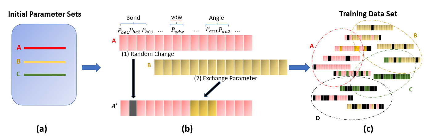
The next step involves score assessment where a score is calculated for each training reference data set is calculated.
| (126) |
| (127) |
Here is the number of geometry sets and corresponds to number of different structures in the geometry set. These structures constitute a specific physical property (Potential energy change as a function of volume change in crystal).
After evaluating the score of every training data ML is used for data analysis. There are three major steps (1) Use Random forest regression to extract important features (2) update initial parameters by k-nearest neighbor (k-NN) algorithm (3) use grid search to get the optimal parameters. In the first step, random forest regression is employed. Where the objective function for minimization can be written in the form of difference between the actual score calculated via ReaxFF and the estimated score via ML:
| (128) |
| (129) |
Here is the number of random samples created and denotes each structure group. The ML model is build by minimizing Eq. 128 and Eq. 129. At the end of ML training important features are extracted which will be used further during grid search parameter optimization. The second step consists of applying the k-NN algorithm to divide the training data into k different groups on the basis of closest distance. For each group scores (Eq. 127) are calculated and the parameter set corresponding to the minimum score is selected eventually modifying the initial parameter set. The modified initial parameter set after the k-NN algorithm is not fully optimized the reason being in a way it is being chosen from the initial data set. Thus grid search parameter optimization is used in the third step which is combined with the extracted parameters from the trained ML model.

Grid search parameter optimization (GSPO) is defined by three parameters , and . Every geometry set (containing various physical properties) has a corresponding ML model with different variations of important features. Depending on the importance of particular feature groups are formed containing elements. In Fig. 37(b) we take , the parameters corresponding to model A are sorted according to their importance (sensitivity). Since first four important parameters are clubbed together forming group A the next set of 4 will be named group B so on so forth. This process is repeated with all the ML models. Since each ML model has varying feature importance levels the groups will contain different parameters. GSPO is then carried out on individual groups by splitting it into m grid points. As each group contains n parameters number the total number of grid points becomes . Getting scores Eq.126 for every grid point for comparison is a laborious task. ML alleviates this issue by selecting test parameter sets from the haystack of different parameter sets. At every group, the scores of test parameters are compared with the Initial sets of parameters obtained from k-NN. If the score of a particular parameter set (in ) is less than the score of the Initial sets of parameters the parameters are updated. However, it’s still a time-consuming task to repeat the process for all the groups (). Since the score does not change much when the group is not sensitive enough. A new cutoff term is introduced which determines when to stop computing score for a particular group and move on to the next. For instance, if GSPO is carried out on group (most important) and group (nest most important). After this GSPO moves on to ML model B.
To summarize while optimizing the parameters of ReaxFF broadly there are three major steps involved (1) Use random forest regression to construct ML models and extract important features (2) Locating probable local minima using k-Nearest Neighbour algorithm (3) Use grid search optimization to optimize the parameters using information from developed ML models. It is important to note that different optimized parameters sets will predict the potential energy decently (in agreement with QM), although their estimation for different physical properties will diverge. The reason is an unavoidable uncertainty is carried out corresponding to a particular physical property during the parameter estimation. Hiroya and Shandan 576 used this approach on a pilot test in which the optimized parameters of ReaxFF were further used to simulate Chemical Vapour Deposition (CVD) of an crystal. The optimized parameters decently predicted crystal structure of even at high temperatures (2000K). Stochastic behavior or the random forest algorithm used in different ML approaches results in hundreds of error evaluations during training for complex training jobs. Where each error evaluation involves minimizing the energy for many molecules in the training data. Recently Mehmet et. al.580 proposed a novel method that employs an automatic differentiation technique from the JAX library developed by Google to calculate the gradients of the loss function. It’s impressive that the efficiency of the gradient-based local optimizer is independent of the initial approximation made for ReaxFF. Given reasonable computing resources, ML-assisted parameter optimization techniques are powerful tools that can be used to simulate wide spectra of reactive MD simulations.
In Non-Adiabatic (NA) Molecular Dynamics (MD) simulations Born-Oppenheimer (BO) approximation breaks down and the electronic and nuclear degrees of freedom can’t be treated independently. These simulations perform a pivotal role while understanding the dynamics of excited states. Recently, supervised machine learning techniques have been employed which interpolates NA Hamiltonian along the classical path approximated NA-MD trajectories581, 582, 583 eventually speeding up NA MD simulations584, 585, 45, 586. NA MD simulations act as a robust resource especially while predicting macroscopic observables such as quantum yield without knowing the mechanism for the larger systems involving strong couplings in which it’s difficult to choose a reaction coordinate587, 588, 589. But they come with a cost of expensive calculations of geometry-dependent forces and energies or the different states. In such situations, ML techniques come to the rescue by predicting band gaps and NA coupling using a small fragment of training data585, 45, 586, 590, 591. To predict the physical properties of materials, unsupervised ML techniques592, 593, 594, 595 has been employed on the trajectories of NA MD simulations while explaining the dominant structural factors 596, 597, 598. Many times Mutual Information (MI) is used to identify unanticipated correlations between many important features. Results from MI are easier to interpret and it is supported by information-theoretic bound which makes it not sensitive to the size of the data set598, 599. These properties make it popular for its application in the chemical regime. For instance, a model of metal halide perovskites (MHPs) based on unsupervised MI unveiled the importance of geometric features as compared to the atomic velocities while predicting Non-Adiabatic coupling (NAC)596.
In a recent study by How et al.600, supervised and unsupervised ML techniques have been used for feature selection, prediction of Non-Adiabatic couplings, and excitation energies of NA MD simulations of metal halide perovskites (MHPs). MHPs have high optical absorption, low cost of manufacturing and long carrier diffusion 601, 602, 603 which makes them an ideal candidate for their use in optoelectronics and solar energy harvesting materials. In order to improve the design of MHPs it is important to develop a computationally efficient and a systematic NA MD which utilizes the theory as well as simulations to predict the physical properties of MHPs. How et al.600 fills this knowledge gap by employing MI on the NA MD trajectory data set of perovskite and extracting the most important features that determine the NA Hamiltonian. The ML model is then validated by checking the performance of the extracted important features to predict the band gap and NAC. Their model showed surprising and counterintuitive results suggesting that the NA Hamiltonian can be predicted by using a single most important feature of the chemical environment information of any of the three elements in . This eventually leads to a drastic reduction in the dimensionality of the original 360-feature ML model developed from ML force fields to merely 12 featured ML models which can produce high-quality NA-MD simulation results which are further confirmed by the present theoretical knowledge about the electronic properties of . This dimensionality reduction technique helps alleviating the high computational cost of ab initio NA-MD and to extends NA-MD simulations to larger, more complex systems and longer time scales.
5.4.2 Quantum-computing enhanced machine learning techniques
Previously variational quantum algorithms (VQAs) have been applied for simulation of small systems 604 with strongly bounded intramolecular forces 605. Most of these approaches relies on complete electronic basis set of the hamiltionian. Smaller coherence times needed in VQA’s makes them ideal fit for the current generation Noisy intermediate scale quantum (NISQ) processors devices. However it is difficult to employ them for simulation of weak intermolecular interactions. As it requires consideration of core electrons (for dispersive forces) leading to a bigger orbital sets eventually requiring large number for qubits. Recently Anderson et. al. 606 resolved this issue by developing a VQA compatible coarse grained model that scales linearly with the system size. Inspired by the maximally coarse grained method 607 their model represents the polarisable part of the molecular charge distribution as a quantum harmonic oscillator in which the parameters are finely tuned empirically to emulate reference polarisability values corresponding to a real molecule. The model contains zero point multipolar fluctuations by definition and thus dispersion interactions exists inherently. Additionally it does not define force laws between atoms and molecules (interaction potentials) which are predicted by using coarse grained electronic structures. Thus the model combines properties from empirical approach and first principle ab-initio approach. Another advantage that this approach has is the number of unique quantum circuits required to measure the given Hamiltonian after considering all possible dipole interactions scales linearly () with the number of quantum oscillators compared to scaling when we consider an orbital based VQE hamiltonian with orbitals 608.
Anderson et.al. 606 showed the solubility of the proposed model by presenting a proof of principle example by calculating London dispersion energies for interacting dimers on IBM quantum processor. While relaxing the harmonic approximation, classical methods heavily relies on path integral and Monte Carlo techniques for efficient sampling of two point correlators for Gaussian states created by harmonic Hamiltonians 609. Since sampling process for non-Gaussian ground states of anharmonic potentials is very expensive anharmonic electron-nuclear potentials remain unexplored using classical computational techniques. VQA base approach shows a quantum advantage as it suffers negligible experimental overhead while performing relaxation of the harmonic approximation. Thus the VQA based approach provides a road-map that includes anharmonicity and higher order terms for simulation of realistic systems which are inaccessible for current classical methods. In conclusion quantum machine learning provides an efficient and accurate way to model realistic systems and may show a quantum advantage in the future.
A detailed theoretical description of the nonadiabatic (NA) process is limited by intricate coupling between nuclear and electronic degrees of freedom (DOF) eventually leading towards adverse scaling of classical computational resources as the system size grows. Although in principle Quantum Computers can simulate real-time quantum dynamics within polynomial time and memory resource complexity. But quantum algorithms have not been extensively investigated for their application towards the simulation of NA processes. A recent study by Ollitrault et. al. 610 proposed a quantum algorithm for simulation of rapid NA chemical process which scales linearly as the system size. Specifically, they propagated the nuclear wave packet across diabatic surfaces having nonlinear couplings (Marcus Model). The algorithm requires three quantum registers. First quantization formalism is used for DOF, so the space and momentum are discretized and encoded in the quantum register. The population transfer between diabatic potentials is encoded in registers and the nonlinear coupling in register. Scaling logarithmic with the precision the proposed algorithm is efficient in terms of the number of qubits requirements. This majestic memory compression while storing the propagated wave function denotes an exponential quantum advantage as compared to its classical counterparts.

The algorithm was applied to simulate NA dynamics of a wave-packet on a simple two one-dimensional harmonic potentials which are shifted in energy by a variable offset. In total 18 qubits were required to simulate this simple model. The characteristic feature of decline in the population transfer of the Marcus model in the inverted region was clearly observed in the simulation, showing an excellent agreement with the exact propagation. Although the simulation was not entirely implemented on the quantum processor the reason is the huge circuit depth of the quantum circuit corresponding to the dynamics parts which requires higher coherence time not attainable by the current generation of quantum processors. But the first part of the algorithm which prepares an initial Gaussian wave packet610 was implemented on an IBM Q device. The extension of this algorithm to higher dimensions is straightforward and a dimensional polynomial potential energy surface (PES) can be encoded with ( is the number of discrete grid points). Current classical algorithms 611, 612 are limited to simulations of molecular systems which are characterized by up to ten vibrational modes. Hence a quantum processor offering approximately 165 qubits with sufficient coherence time would alleviate this hurdle thus providing an immense quantum advantage while understanding fast chemical processes involving exciton formation, inter-system crossings, and charge separation.
Although Quantum Machine Learning (QML) shows quantum advantage in electronic structure calculation, its application towards force field generation remains unexplored. A recent study by Kiss et. al.613 learns a neural network potential energy surface and generates a molecular force field via systematic application of parametrized Quantum Neural Networks (QNN) techniques on the data set generated from classical techniques. The proposed QNN model was applied on single molecules and the results show the competitive performance of the QNN model with respect to its classical counterparts. Additionally, the results suggest that a properly designed QNN model exhibits a larger effective dimension resulting in fast and stable training capabilities. This potentially hints towards a possible quantum advantage of QML’s application in force field generation
5.5 Drug-Discovery Pipeline and pharmaceutical applications

To deploy machine learning or deep learning algorithms for computer-aided drug discovery (CADD) 615, 616 it is important to access large molecular databases wherein such structural information about the target (receptor) and/or drug (ligand) candidates may be found. Such databases are screened to generate prospective hits based on either binding affinity with the target above a threshold for structure based protocols or by looking at chemical similarities with previously known bio-active candidates for ligand-based protocols. For the second category, chemical databases like PubChem 617, 618, ChEMBL 619, Drug-Bank 620, DUD-E 621 etc may be good choices. DUD-E contains many decoys (ligands/drug candidates which shows similarity in properties but are not topologically similar in structure) which may be useful for testing and validation of the trained models. For the first category wherein physical information about the target protein is necessary, databases like UnitProt 622, PDB623, 624, 625, PDBbind 626 may be a useful resource. Combination databases BindingDB 627 which contains experimental data for several ligands and targets together have also been employed extensively too. Most of these databases do encode the structural/physico-chemical attributes of the candidate molecule and/or the target into computer-inputable format which are either numerically describable or string-based. These are called features or very simply molecular descriptors and often depending on the choice of the user other molecular descriptors can be generated using the accessed structural information with libraries like RDKit etc. For the ligand/drug generic features like number of atoms, molecular weight, number of isomers etc are often called as 0D features as they do not describe the specific nature of the connectivity of atoms within the molecule and remain oblivious to conformational changes. 1D features like SMILES 628, 629, 630, SELFIES 631, 632, SMARTS 633, 634 which encodes the connectivity pattern within the molecule using strings are quite commonly used. On the other hand, numeric features are based on fingerprints which usually represent the molecule as a binary vector with entry 1 (0) corresponding presence (absence) of certain prototypical substructures/functional groups. These are further divided into many categories like circular fingerprints like ECFP 635 which are extremely popular as they are quickly generated, Morgan fingerprints 636, Molecular ACCess System (MACCS)637, Tree based fingerprints 638, Atom pairs 639, 640 to name a few. Graph based 2D descriptors641, 642 are also commonly used with the atoms in the molecule represented as vertices and the bonds between them as connectivity pattern. Adjacency matrix derived from such a graph can act as a molecular descriptor. Fig. 39(b) shows the an example for representing a given molecule in the commonly used 1D and 2D formats. However, these 1D and 2D descriptors even though widely used are often less sensitive to stereochemistry within the molecule which may be important for evaluating binding proclivity with the target. 3D descriptors are useful for this purpose as detailed structural information like dihedral angles are important for this encoding643, 644. Higher dimensional encoding with information like specific conformational state, interaction with the solvent or the background residues of the target may also be used to enhance the predictive capacity of the model643, 644.
5.5.1 Structure-based drug designing protocols using classical machine learning techniques
We first see the performance of machine learning techniques on the structure-based drug designing protocols (see Fig.39 (a)). The primary goal for such studies is to determine whether the prospective candidate molecule can bind effectively (and thereafter evaluate the binding pose and compute the binding affinity) to the target receptor given that the structural information about the target protein is available from prior experimental (like X-ray, NMR etc) or theoretical studies 615, 644. Even though experimental assurances are the most trusted means of evaluating such an interaction , yet simulation of the process gives a window into understanding the interaction between a prospective candidates with the desired target relegating the need for direct labor and money intensive experimental verification at a later stage before clinical trial thereby leading to efficient screening. Recently, convolutional neural-network (CNN) (Basic theoretical formalism discussed in Section 3.3.2 and recurrent neural network based models (RNN) (Basic theoretical formalism discussed in Section 3.3.3) are being used to investigate the process. In a celebrated work by Ragoza 339, 3D conformational images of the protein and molecule (ligand/drug) is taken and trained with a CNN to identify which poses are suitable for binding and which are not. The SAR-NRC-HiQ dataset was used 645 containing 466 ligand-bound receptors (proteins). Two training sets are generated from it by re-docking using Smina 646 and labelled using the Auto Dock Vina scoring function 647. These re-docked 3D structures are discretized into grid near the binding-site with a length of 24 Å on either axis and 0.5 Å resolution. The ligand and protein atoms within each such grid points were differentiated. This served as input to the CNN. CNN model used had an architecture of five hidden layers with ReLU activation and additional max pooling layers. The model was trained using Caffe Deep Learning framework 648 minimizing multi-dimensional logistic loss function using gradient descent as the training algorithm. CNN outperformed AutoDock Vina scoring in pose-prediction ability i.e. grouping which poses affords a good binding affinity. The superior performance of the model was upheld for virtual screening too. Compounded datasets by combining training examples from both the tasks were used and the CNN model based training was found to be as effective as their separate counterparts. Even though the CNN was not trained on mutated protein datasets for binding affinity, yet it was able to register the amino acid residues within the protein critical for binding which afforded an easily interpretable visualization of the features that the network is learning. The work envisioned developing protocols to perform tasks like pose-ranking, binding affinity prediction , virtual screening using a highly multi-task network trained on much larger dataset which can ameliorate its performance even more.
In a similar work Yang-Bin Wang 649 developed a computational model with memory based on LSTM to construct a framework for drug-target interaction. Information about the drug-target pairs were obtained using Kegg 650, DrugBank 651 and Super Target databases 652. Four classes of targets were considered i.e. enzymes, ion-channels, GPCRs and nuclear receptors. From the dataset curated from the above bases, the drug-target interaction pairs with known affinities are set as positive examples while the remaining are treated as negative examples. The structural features of the protein was described using Position Specific Scoring Matrix (PSSM) 649. For a protein consisting of amino acids , PSSM is a matrix with the (i,j) th element of the PSSM denotes the probability of mutating the ith amino acid in the sequence with the native amino acid from the list of 20. The PSSM was constructed using PSI BLAST 653. Legendre moments using the elements of PSSM was then constructed to remove redundancy in features. At the end 961 features were obtained for each protein sequence. The structural features of the drug was encoded molecular fingerprints. PubChem database was used for this purpose which defines 881 sub-structural features. As a result each drug/ligand was represented by an 881 dimensional Boolean vector denoting the presence or absence of these tagged molecular substructures. The total 1842 dimensional vector (881 + 961) for the molecule and the receptor target was reduced to 400 size feature vector using sparse principal component analysis (SPCA). This combined feature vector was fed into the classifier. Multiple LSTM layers were stacked to get a deep LSTM setup i.e. 4 hidden layers with 36 neurons were used. Overfitting was compensated by using dropout of randomly chosen neurons during the training process. Different performance metrics were used like ACC, true positive rate or even the standard AUC as defined before 654. Both hyperbolic tangent and logistic sigmoid was used as the activation function depending on the case (see Section 3.3.1). The output layer being a classifier uses a softmax. The method attained great accuracy across all performance metrics for all the 4 classes of drug-target chosen in comparison to traditional machine learning techniques or even multi-layer perceptrons. The multi-layer perceptron they trained had the same number of hidden units as the LSTM network being used for a fair comparison. The method performed reasonably well even with small training sample size like 180 as was available for the nuclear-receptor family. In another recent work by Zheng 655, a deep learning algorithm is developed with both CNN and LSTM. The target/receptor proteins is processed into a fixed length feature vector using a dynamic attentive CNN. 16-32 filters and 30 residual blocks were used in the construction of the dynamic attentive CNN 656. The drug candidate was represented as a 2D matrix similar to 657. This is processed using a self-attentional LSTM network 655 known as BiLSTM which extracts features. The number of hidden layers in the BiLSTM network was 64. Three kind of databases were used for numerical experiments. The first is DUD-E 658. This dataset has 102 target receptors across 8 protein families. Each receptor has 224 active drug molecules and 10,000 inactive ones. The final dataset curated from this database had 22,645 active drug-protein interaction pair examples and 1,407,145 negative ones. The second database used was Human 659 containing 1,998 unique proteins and 6,675 interactions. The third database used is Binding DB 660 which contains experimental results of binding affinities. The dataset curated from this had 39, 747 positive examples and 31,218 negative binding interaction pairs. The two feature vector of the target and the protein are combined and fed into a classifier which generated a probabilitty vector from it using sigmoid activation. This probability vector was then minimized against the data label of positive and negative interaction pairs using cross-entropy with regularization. The metric used to evaluate the final performance of the model is area under the ROC (Receiver-Operating Characteristic)661 curve. This metric is often abbreviated as AUC in literature. Receiver-operating characteristic curve (ROC) enrichment metric (RE) is also used for DUD-E dataset. For the Human dataset, the method achieved 98.7 % for AUC outperforming all traditional methods like Random Forests, Support-Vector Machines etc. For DUD-E dataset, the method outperformed Vina 647, AtomNet 662 to name a few. On BindingDB with seen and unseen drug-target pairs too , the model outperformed all traditional competitive algorithms. Visual demonstration of which amino acids residues of the target and what structural features/moieties in the drug are important for interaction was also provided.
5.5.2 Ligand-based drug designing protocols using classical machine learning techniques
Next we move onto to ligand-based drug designing protocols (see Fig.39 (a)). The objective of these methods is to analyze what kind of prospective drug/ligand candidates obtained by screening compound libraries share similar structural features with previously known drug candidates (used as reference) against the given target. In this paradigm one operates under the premise that ligands with such features will have similar bio-activity too against the said target. These methods are therefore useful when direct structural information of the target is not available 615, 644 but bio-activity of some reference compounds against the target is known from previous domain knowledge. One most commonly employed technique in this category is constructing quantitative relationship between structure and activity (QSAR). QSAR is the analytical quantification to the degree to which structural related molecules will share isomorphic bio-activity and hence allows prediction of the behavior of the newly screened compounds against the specified target. This facilitates the identification what structural features are responsible for the activity and hence provides insight into rational synthesis of drugs in future.
The first report for the use of deep-learning models in QSAR prediction after the publically accessible Merck challenge was due to Dahl 663. QSAR studies mainly focus on understanding what chemical composition and structural features of the prospective molecule of choice (ligand) might have desired pharmacological activities against a chosen target (receptor). The study by Dahl focused mainly on the effectiveness of multi-tasking while designing architectures for neural-networks (Basic theoretical formalism discussed in Section 3.3). Multi-tasking refers to the ability of the network design wherein different outputs of interest are simultaneously retrievable. For instance, in the aforesaid study a single-task network would be training using molecular descriptors obtained from compounds within a single assay (data-set) as input features and using the activity of the said molecule as a performance label for comparing the output. However, this model of training requires huge data assemblies from single assays alone which may not always be available. To circumvent the issue, the authors of the aforesaid study combined data from multiple assays using an architecture in the final output layer wherein individual neurons are dedicated to each assay. The same molecule may have appeared in different assays with different activity labels. For any given such molecule, the input feature vector is the molecular descriptor. The output at each of the neurons in the final layer are the activity/inactivity classification values learnt by the network for each assay. This output is then compared against the recorded activity label obtained from the corresponding assay for back-propagation. The study used data from 19 such assays from PubChem database (see Table I in 663) with each assay containing compounds. The molecular descriptors used were generated using Dragon software664 as a feature vector of length 3764 for each compound. Although the model is a binary classification study, the performance metric used is AUC as defined before. The network was trained using Stochastic-Gradient Descent algorithm with momentum and the problem of over-fitting due to many tunable parameters was eschewed using drop-out 205. It was seen that the Deep-learning network used outperformed traditional machine learning models in 14 out of the 19 assays. Among these 14, multi-task networks outperformed single-task models in 12 of the assays. These favorable results were retained by grouping similar molecules across different assays into a customized composite data-set. The depth of the neural network/addition of more hidden layers did not always produce improvement in the performance of the multi-task network which the authors attribute to smallness of the data within each assay. All the deep-learning models used handled reasonably well correlated features in the input feature vector. In a related study Ramsundar .665 resolved certain questions about the efficacy of multi-task neural networks in virtual screening of candidate molecules against several targets using extremely large data-sets. 259 assays were used and divided into 4 groups - PCBA, DUD-E658, MUV, Tox21. Together all these databases had 1.6 M compounds. The validation scheme used is AUC as before and the feature vector of the studied compounds were ECPF4 fingerprints635. All such collection of fingerprints for the molecule were hashed into a single bit vector. The trained network as before is a multi-task classifier with each neuron at the output layer having a softmax activation666 corresponding to each assay. The study found that such multi-task NN performed better than several ML models and the performance metric can be improved with increasing number of tasks and/or increasing the volume of data per task. Certain data-sets in the study showed better performance than others which were attributed to shared set of compounds among such databases. However the biological class of the target receptor did not affect the performance metric too much. The study concluded by saying that extensive data-sharing among proprietary databases needs to happen to benchmark the performance of such models with bigger data-sets. Another study which thoroughly benchmarked the performance of deep neural networks against a commonly used machine learning model like Random Forest (RF) was due to Ma 667. The report used 15 Kaggle data-sets for training and another 15 for validation too. Each such data-set had around candidates as molecular designs for drugs each labelled with response activity against designated target(s). The type of descriptors used for each of these molecules included combination of atom pairs and global donor-acceptor pairs 668 as input feature vectors. The report used the squared Pearson correlation coefficient (R2) 669 between observed and predicted activities in the testing set as the preferred metric of performance. The study showed that there was a mean improvement in R2 of 0.043 when using deep-neural network as opposed to RF against arbitrarily selected parameters. 4 of the data-set showed dramatic improvement in favor of deep-neural network whereas one favored RF. When refined parameter set was used instead of arbitrarily chosen ones, the trend is retained with an expectedly higher mean improvement of 0.051. Increasing the number of hidden layers and also number of neurons in each such hidden layer displayed a R2 in favor of deep neural network. Changing the activation function from sigmoid to ReLU 666 also favored the deep network model for 8 data-sets. R2 was found to also favor networks when it is not pre-trained.
5.5.3 Machine learning and drug-induced toxicity
Another area wherein machine learning algorithms are important is identifying if a particular drug when administered in a biological medium would be toxic or not. Such adverse effects due to an administered drug may lead to serious health complications culminating in the eventual withdrawal of the drug during development/testing or even post-marketing thereby leading to wastage of resources. Many such studies has been initiated like in 670. The earlier investigations primarily used machine learning methods. This can be exemplified from the work of Rodgers 671 which created a model using k-nearest neighbor (kNN) (Basic theoretical formalism discussed in Section 3.2.4) for identifying whether a drug candidate from Human Liver Adverse Effects Database (HLAED) belongs to two categories- hepatotoxic in humans or not based on labelled markers from five liver enzymes. With a dataset of over 400 compounds, the algorithm was successful in classifying with a sensitivity of 70 % and a specificity 90 %. The model was extended to test unseen cases in World Drug Index (WDI) database and Prestwick Chemical Library (PCL) Database with good success ratio. To do so, a compound similarity metric based on Euclidean norm between molecular candidates were used and an applicability domain threshold was constructed using the metric. Predictions for candidates with similarity scores outside the applicability domain threshold were considered unreliable. Chemical features like aromatic hydroxyl units in drugs like Methyldopa 672 or pyrimidyl units in drugs like Trimethoprim 673 were identified to play a key role in the assignment of high hepatotoxic activity of the respective drugs as they are prone to oxidation and can form hapten adducts with cellular proteins. In yet another study 316 a classification task among molecular candidates were designed using Support-Vector Machines (Basic theoretical formalism discussed in Section 3.2.7) with the Gaussian Radial Basis Function (RBF) as the kernel to group molecules into active and inactive categories with respect to susceptibility to induce phospholipidosis (PLD). Phospholipidosis refers to intracellular accummulation of phospholipids induced by drug candidates when they bind to polar phospholipids in the lysosome 674. The model was trained by curating dataset from three databases National Institutes of Health Chemical Genomics Center (NCGC) Pharmaceutical Collections (NPC)675, the Library of Pharmacologically Active Compounds (LOPAC) and Tocris Biosciences collection and the target cell used was HepG2 676. The model developed was found to accomplish the selection task with high sensitivity and specificity as seen from the AUC metric. The training was found to be sensitive to the nature of molecular descriptors used and also to the size of the dataset. Certain simple chemical attributes like size of hydrophillic moieties are often used as indicators to characterize if a drug can induce PLD. Such features even though showed correlation with the identified active compounds in some cases but did not agree on some others. On the contrary features like presence of positively charged nitrogen center correlated well across the entire dataset. Identification of such features may be important to chemist for avoiding or replacing such structural moieties during the early developmental stage of the drug.
Deep learning models have also been deployed for the said purpose. In a recent one using artificial neural network, toxicity due to epoxide formation is thoroughly investigated341. The study identified among a given set of drugs/ligands and targets which drug is susceptible to be epoxidized with natural oxidants in the biological medium by oxidants like cytochrome P450. Formation of such epoxidized metabolities can be harmful for the body as has been explicitly noted for the case of an anti-epileptic drug like carbamazepine 677 which after epoxidation binds to nucleophillic sites within a protein forming a hapten adduct thereby triggering immune response678. The product of such reactions need not always be an epoxide as the study suggests from previous reports 679 for drugs like N-desmethyl triflubazam wherein a DNA adduct is formed post a transient epoxidation. The neural-network model used in the study not only decides if a given drug is epoxidizable but also focuses on identifying if the site of epoxidation (SOE) is a double bond or an aromatic ring. It further delineates such sites from site of hydroxylation (SOH) which shares some key structural features with SOEs and can also potentially lead to harmful oxidation products. The Accelrys Metabolite Database (AMD) was used from which a dataset of 389 molecules were curated having toxicity labels. These molecules had 411 aromatic SOEs, 168 double bond SOEs and 20 even single bond SOEs. Non-epoxidizable molecules were also included in the set thereafter to afford a proper distinction. To describe each bond within the specific molecule 214 molecular descriptors/features were identified- 89 each for the left and right atom sharing the bond, 13 specific bond descriptor and 23 overall molecular descriptors. The neural network used had 1 input and 2 output layers . The top output layer was for the molecular epoxidation score whereas the last one for the specific bond epoxidation score. The training data involved using labelled binary vector within the molecule with the designated SOE marked as 1. Cross-entropy minimization was used as the cost function. The final metric of performance as before was AUC. The model outperformed logistic regression and other competitive algorithms in all departments like identification of SOEs, differentiation of SOEs and SOHs etc. The model could correctly identify SOE in carbamazepine which is absent in substitutes like oxcarbazepine with similar functionality, in the furan ring of furosemide 680 and in severely hepatotoxic sudoxicam vs its less problematic cousin like meloxicam 680. More such examples can be found in specialized topical reviews like 670.
5.5.4 Power of quantum computers and quantum-computing enhanced machine learning techniques
As discussed in other domains, quantum computing enhanced machine learning techniques are also beginning to gain attention in the overall drug production pipeline. An early review 681 identified the efficacy of quantum computers to the drug discovery process by noting the key areas wherein quantum computers can impact. The study reported that for structure based drug designing protocols, quantum computers may help in understanding the structure of target protein sequence better. It claimed that using both gate model of quantum computing and quantum annealers, simple problems like the Miyazawa-Jernigan model were investigated for understanding the dynamics of protein folding for smaller peptides 682. Unfortunately such model problems may not accurately assess the real situation in all cases especially for complicated situations like the presence of several protein conformations with minimal free energy difference thereby rendering them accessible via thermal fluctuations or how the native 3D conformation of the protein is sustained due to its interaction with the surrounding media. In most cases for biologically significant proteins, crystallized 3D structure is not available in the database due to sheer size of the protein and/or lack of solubility etc 615. As a result structure-based designing protocols are often thwarted. Better computational models for predicting the protein structure is therefore necessary and can influence the drug-discovery pipeline immensely. Banchi 683 used Gaussian Boson Sampling to identify the highest affinity binding poses of a given ligand with the active centre of the target. The primary workhorse of the protocol is to map the active centre and the ligand onto a pharmacophoric feature space of few descriptors. Each such descriptor corresponded to a vertex in a graph and the edges defined the Euclidean distance between the corresponding structural motif in the lowest energy 3D geometry. The resultant encoded graphs were then used to construct a binding-configuration graph wherein structural features of the ligand and the target that are compatible to bind are represented by a weighted vertices. The maximum-weighted clique (a closed sub-graph) within the binding-configuration will be the preferred binding pose. Such configurations are identified with high-probability using a Gaussian Boson sampler with the input state of photons being in squeezed states and identifying the detector wherein the photon appears at the output. Such detectors corresponds to vertices on the binding-configuration graph. If the combination so-attained at the output is not a clique then the authors have defined greedy shrinking of vertices or expansion of vertices by probing the local environment to modify the search space for next iteration. Recently, an efficient hybrid-variational algorithm amenable to NISQ architecture has also been proposed which using an -sequence amino acid can construct a sample of the lower energy 3D-conformations684. Previous reports tackling the same problem were either inefficient or offered problem specific solutions 685. The work represented the given sequence by stacking monomeric units on a tetrahedral lattice. 4 qubits were assigned for each of the 4 different directions the lattice could grow from a given monomer. New ancillary qubits were also used to define the interactions between l nearest neighboring (l-) monomeric units. A graph hamiltonian was constructed with these interactions and the self-energy terms of each residue. Overlapping positions of the amino acids were avoided by including penalty terms corresponding to such assignments. The ground state of this hamiltonian is the most stable conformation. To solve the problem, a variational circuit was constructed parameterized by tunable rotation angles of both the single-qubit and entangling gates involved. The various bit-strings obtained from the measurement of the circuit encoded the 3D structural arrangement of the amino acid residues in the tetrahedral lattice and the energy distribution would highlight the relative stability of these various arrangements/conformations. The circuit was optimized variationally to selectively enhance the chances of sampling the lower energy conformations corresponding to tail of the aforesaid energy distribution. The number of qubits in the method scales as and the number of terms in the hamiltonian is . The model was tested on 10 amino acid peptide Angiotensin using 22 qubits and also on a designed 7 amino acid neuropeptide using 9 qubits on IBMQ processors. In the former the probability of collectively sampling all the lower energy conformations was reported to be 89.5 % which augmented further with increase in the number of measurements.
However recently a work from Google’s DeepMind (UK) 686, have made enormous strides in predicting the 3D structure of a peptide from just a given sequence of amino acids solving this 50-year old grand challenge. Even though the algorithm uses a neural-network architecture trainable on a classical computer (and hence is not a quantum-computing enhanced algorithm), yet the performance of the method is so good that it deserves a special discussion. This novel algorithm has won the CASP14 challenge which involves a blind assessment of the efficacy of structure determination from amino acid sequence for proteins/peptides whose structure has been recently solved through explicit experimentation yet has not been publicly released in common databases. The neural network design is broken down into three components. The first component in the neural network architecture takes as input a 1D sequence of amino acid residues and searches multiple databases to generate multiple sequence alignments (MSAs) which are essentially sequence of previously identified amino acids closely resembling the target one and understanding the evolutionary history of the mutation of these MSAs.

This is important to derive information about structural proximity between amino acid pairs which shows correlated mutation. This component then generates a template 3D structure also called pair representation as an initial hypothesis that is to be modified at later stages. The next functional unit is called the Evoformer and is the heart of the design. This takes as input both the pair representation and the MSA and subsequently refines the representation of each self-iteratively using the architecture of transformer 459. The third block takes the refined MSA and the pair representation and generates a 3D structure which is essentially cartesian co-ordinates of the individual atoms i.e. the native 3D conformation of the protein/peptide. This process is repeated several times by feeding back the 3D structure into the Evoformer block until convergence. The final prediction seems to have surpassed all previously known methods with an accuracy of 0.95 Åroot-mean square error from the target structure for 95 % of the residues. This will definitely be a landmark study and for years to come one has to investigate the efficacy of the method for antibodies , synthetic peptide sequences for which evolutionary data to generate the initial MSA will be scarce. This method will positively impact understanding protein-protein interactions and also bring in new insight in diseases like Alzheimer’s and Parkinson’s. For structure based drug-discovery since at least one method exist now which can determine the 3D conformation efficiently thereby massively speeding up the product development pipeline, quantum computers can now help in understanding the drug-protein affinity and molecular docking mechanisms. The review by Cao 681 already identifies this possibility by noting that with algorithms like quantum phase estimation on fault-tolerant devices and variational eigensolvers for near term devices, we are capable of computing the potential energy surfaces of larger molecular systems efficiently and hence force-field calculations as is required for understanding molecular docking will also be greatly impacted.
For QSAR studies too, benchmarking the performance of quantum computer against classical processors has been documented recently in the work of Batra 317. The authors have used several molecular databases to identify prospective ligands for diseases like M.Tubercolosis, Krabbe disease, SARS-CoV-2 in Vero cells , plague and hERG. With the curated data from the compound datasets feature vectors were constructed and used for binary classification of the compound in active or inactive using kernel-based SVM techniques (see Section 3.2.7 for basic theoretical formalism). The authors used several techniques to reduce the size of the feature vector such that the classification can be performed on a NISQ device ( was used) using Qiskit. It was seen that for most datasets comparable accuracy on a quantum computer was attained too using the feature reduction techniques employed by the authors. A hybrid quantum-classical approach was also used for high-throughput virtual screening data screening with good accuracy and slightly faster run time for processing the data on a quantum computer than on a classical computer. Representative data from the study is displayed in Fig. 40.
Beyond the precincts of academic research, even the interest of industrial players on quantum-enabled technologies seems to be escalating rapidly. The report by Zinner 687 have identified that 17 out of 21 established pharmaceutical companies and 38 start-ups are directly working on enhancing and ameliorating the technical challenges in the drug discovery pipeline using quantum computers. 75% of such companies so far have been identified to be geographically in Europe and North America. The cumulative funding received by all the start-ups as per the report 687 is €311 million with the top five funded start-ups being Cambridge Quantum Computing, Zapata, 1QBit, Quantum Biosystems and SeeQC. Most of the activity is directed towards virtual screening for ligand-based drug designing protocol and subsequent lead optimization.
The report from Langione 688 and Evers from McKinsey 689 also systematically delineates what pharmaceutical industries should do to prepare themselves attain a favorable position in order to leverage the quantum revolution. Both the reports agree that bio-pharmaceutical companies should start now to reap the benefits of early movers advantage. In fact 688 mentions that it might be possible that tech-giants equipped with quantum computers with higher number of qubits and better noise-tolerance might enter the race of in -silico drug discovery in the future relegating the task of post-design synthesis, clinical trials and commercialization to pharmaceutical companies. That can lead to a situation wherein companies may race to patent the best molecule that are responsive to a particular disease. However pharmaceutical companies are at an advantage here due to years of experience with computational drug-designing protocols. So strictly they do not have to change the inherent model or the business goal they already follow. They will likely be using a more capable device like a quantum computer to attain that goal. In order to avoid such undue competition, pharmaceutical companies should start now by assessing and answering few key questions about the probable impact quantum computers are likely to have on the workflow and the specific product design the respective company is targeting. This can happen by understanding what are the key areas where development can be sought in the product design model the company is following and more importantly if those areas fall into the category of problems that can be solved efficiently on a quantum computer. The key directions to think would be would a quantum-computer enabled business provide an unprecedented value to their supply-chain or an undue advantage to their competitors. If the analysis is positive, one needs to then think of the time scale of such developmental changes and whether the resources the company has access to would be enough to sustain entry into the domain. Some of above resource overheads can be solved through appropriate memberships through consortium like QuPharm that categorically specializes in the designated area. QuPharm, as an organization was developed by many member pharmaceutical companies for specifically understanding and optimizing the benefits the quantum revolution can have on the pharmaceutical industry. The consortium is known to have a collaboration with Quantum Economic Development Consortium (QED-C)687. Hardware needs can be sorted through collaborations with end-to-end technological providers like Google, IBM, Honeywell, Rigetti, Xanadu etc each of which have quantum computers of varying architecture and even on different platforms and have even promised to develop larger scale ones in near future. For example Amgen, a pharmaceutical company has declared collaboration with both Amazon Braket and IBMQ 687. Boehringer, another pharmaceutical has established collaboration with Google QuantumAI to develop algorithms for molecular dynamics simulation 687. New software solutions are necessary to interface with the quantum hardware for which commercially available varieties like Qiskit (IBM), OpenFermion (Google), tKet (Cambridge Quantum Computing) can be leveraged. Companies can also initiate partnerships with firms like ProteinQure, GTN, Rahko, Qulab etc which are developing softwares to specifically cater to advancing quantum-computing algorithms for drug discovery . Classical computing algorithms have also benefited from the ideas that were synthesized to initiate a rapid discovery of quantum algorithms over the last few years. Companies like Qubit Pharmaceuticals, Turbine etc are developing such approaches and combining them with machine learning. Such collaborations with global and local companies with specialized expertise can result in engineering custom solutions to tackle specific problems during the drug discovery pipeline. Pharmaceutical companies can thus immensely benefit from such collaborative ventures.
Partnerships can be built with other pharmaceutical companies or start-ups too to share expertise and develop mutually beneficial quantum computing based drug-development protocols. The report by Zinner 687 has identified 17 pharmaceutical companies with publically disclosed collaborations with at least 12 start-ups. All the pharmaceutical companies are members of QuPharm, NEASQC etc. Among the big pharma corporations Merck (Germany) has invested €4 million on start-ups like SeeQC and has disclosed active collaboration with Rahko, HQC 690, 691. Merck (USA) has made financial investment in Zapata 692. Non-equity partnerships like that by Amgen with QSimulate to develop advanced molecular simulation tools or like that by AstraZeneca with ProteinQure to design amino-acid sequences have also been seen 693. Some new collaborations are also announced which depicts not only the prospective promise associated with the technology but also the seriousness of the industry players. For example, Cambridge Quantum Computing have announced a collaboration with CrownBio and JSR LifeSciences about using quantum machine learning algorithms to identify multi-cancer genes biomarkers 694 which can positively impact bioinformatics research. Apart from this, it would also be beneficial for pharmaceutical companies to collaborate with scientists in academia. Adopting a strategy that allows effective co-operation among all involved parties internal and/or external beyond the traditional organizational structure will accelerate growth and foster efficient and fast sharing of resources and knowledge which can otherwise be harder to access due to institutional barriers. The reports 688, 689 identify that recruitment of skilled technicians and professionals with training in developing algorithms on a quantum computer is necessary for pharmaceutical companies to enhance quantum-enabled research. The report by Zinner 687 conducted a thorough search across 21 pharmaceutical companies with a combined revenue of €800 billion in 2019 and reported that only about 50 employees were found designated to quantum-enabled technology. This is partly because quantum computing is an emerging technology and hence such a skillset may not be readily available among the usually hired talent pool of the pharmaceutical industries688. Companies like IBM which holds outreach programs and workshops in quantum computing interfaces like Qiskit can be a useful resource. The other alternative might be looking into developing specialized programs internally to train scientists and engineers once hired.
6 Insight into learning mechanisms
Despite the enormous success of machine learning coming from network based models with large number of tunable parameters, little progress has been made towards understanding the generalization capabilities displayed by them 695. The choice of hyperparameters in these models have been based on trial and error with no analytical guidance, despite it showing enormous potential in analyzing data sets. Physics on the other has provided us with white box models of the universe around us that provides us with tools to predict and examine observed data. Intuition from statistical mechanics have helped provide understanding with respect to the learning limits of some network models. Seminal contributions in this regards include methods from spin glass theory, that have been used to extensively study associative memory of Hopfield networks 696 and Valiants theory of learnable models that introduced statistical learning into the then existing logic based AI 697. Another major contribution comes from Gardners usage of replica trick to calculate volume in the parameter space for feed forward neural networks in the case of both supervised and unsupervised models 698, 699. The problem of learning was also shown to exhibit phase transitions in reference to generalization and training efficiency 700. A typical example of one such parameter is the ratio of input size to the number of model parameters. A diminishing value usually results in overfitting while a large allows for successful generalization. The reader is encouraged to refer 701, 702, 703 for some of the early works that made use of statistical physics to understand multi layered network learning

We will see that some self averaging statistical properties in large random systems with microscopic heterogeneity give raise to macroscopic order that do not depend on the microscopic details. Learning these governing dynamics can play an important role in tuning the performance of machine learning techniques. One of the tools that provides an analytical handle in analyzing these details is the replica method 704. Replica methods have been used to explore the teacher-student model to provide information theoretic best estimates of the latent variables that teacher uses in generating the data matrix handed over to the student 705. This problem can be specialized to the case of providing a low rank matrix decomposition matrix of underlying input data. Interest into statistical methods have stayed dormant since 1990, due to the limited tractability of algorithms used in learning. It was sparked again with the contribution of Decelle 706 to use spin glass theory to study stochastic block model that played a major role in understanding community detection in sparse networks. They observed second order phase transitions in the models that separated regions of efficient clustering when solved using belief propagation algorithms 707. For a comprehensive list of physics inspired research in the machine learning community, refer 708.
Generative models are suitable for feature extraction apart from doing domain sampling. Within every layer of one such network, one could imagine some form of feature extraction being made to provide for a compact representation, which might later be used by generative models to learn the distribution of classifiers to do prediction. We point towards this feature extraction as the central idea for relating machine learning to renormalization group. We investigate to see if concepts like criticality and fixed points have something to reveal about the nature in which learning happens in the framework of deep learning and machine learning in general. Figure 41 provides a schematic sketch of the methods that have been primarily explored in studying network models. In here we shall restrict our attention to cavity methods, Renormalization group and Replica methods. Refer 709 for a thorough exploration of Message Passing Algorithms.
A somewhat non rigorous argument for the remarkable working of these machine learning algorithm comes from noting the following two observations. Consider a vector of input size taking values and thus can span a space of possible configurations. Despite this being exponentially a large space for image datasets, we have managed to build relatively small networks that learns to identify the features of the image accurately. This is to be attributed to the realization that the class of relevant images comes from a relatively small subspace that is efficiently learnt by the neural network with relatively fewer nodes that scale as instead 710. This is much similar to how low energy states of interest of hamiltonian mapping to small subspace of the Hilbert space. This simplification comes from the Hamiltonian having a low polynomial order, locality and symmetry built into it . Secondly, despite the vastness of all possible inputs that can be generated, most input data can be thought of coming from a Markovian process that identifies at each stage a select set of parameters. Thus the work of a deep learning machine would be to reverse some form of heirarchial markovian generative process using some minimal statistic function (A function is minimal statistic if for some random variables and we have ) that retains the features of the probability distribution by preserving mutual Information.
The methods in the following subsection describe its working in the context of Ising model, so we start by describing one briefly. Ising is a model for representing classical spins or magnets arranged in a 2d lattice whose interaction with one another is quantified by the strength of the coupling. Each spin takes a binary configuration of choosing to align up or down. At low temperatures spins prefer aligning in the same direction forming a magnet. At high temperatures the thermal fluctuations kill any order within the system causing them to arrange chaotically with no net observable magnetic field. A general Ising Hamiltonian is given by,
| (130) |
where indicates the sum over nearest neighbour pairs. The probability of any given configuration is determined by the Boltzmann distribution with inverse temperature of the system scaling the governing Hamiltonian. Expectation values of observables correspond to averages computed using the distribution. Given any observable the expectation value at a given inverse temperature is given by,
| (131) |
6.1 Replica Method

Replica method is a way of computing self averaging expectation values of observables such that is a minimizer of where is the distribution some input space. A typical example of would be the cost function of a learning problem and would be the dataset used for training in the problem. Figure 42 provides a schematic representation of the use of replica method. Here we shall be explore it in the context of Ising Hamiltonians. Consider the Ising model of N spins, given by the following Hamiltonian,
| (132) |
where the connectivity matrix entries has been sampled independently from a Gaussian distribution with zero mean and variance . The spins take values from . In a bath of inverse temperature this results in an equilibrium distribution that is governed by the Gibbs distribution given by,
| (133) |
where Z is the partition function. We would like to analyze the structure of low energy patterns that is independent of the realization of the couplings in the large limit. Properties of disordered system can be learnt by studying self averaging properties (have zero relative variance when averaged over multiple realizations) . Steady states emerge in the large limit as a result of diverging free energy barriers causing time average activity patterns that no longer look like Gibbs averaging, due to broken ergodicity.
To study the patterns encoded within the Gibbs distribution, we start with computing the free energy average over all the realizations of . This involves computing expectations of a logarithm which can be simplified using the following Replica trick.
| (134) |
Evaluating is much simpler as this can be expressed as an average over replicated neuronal activity, i.e,
| (135) |
where denotes the set of replicated spins over which the averaging is done. The Gaussian integrals can be easily evaluated resulting in,
| (136) |
where the overlap matrix . Minimizing the free energy amounts to retaining patterns with maximal overlap. The non zero averaging can be interpreted as certain patterns being promoted within replicas and enforced across different realizations of . The minimization of free energy gives a self consistent equation for ,
| (137) |
where refers to averaging over the distribution , where . The hamiltonian is symmetric with respect to permutation of indices and thus for all . Minimizing the free energy with respect to the variable gives a self consistent equation,
| (138) |
where is a random variable with Gaussian distribution of mean zero and variance . For i.e, high temperature, is the only solution, representing a paramagnetic phase while for , i.e, low temperatures we have a continuously raising value from zero, suggesting a phase transition. However the replica symmetric saddle point solution for derived for the Ising Hamiltonian is unstable and is thus inconsistent with physical predictions 711.
6.2 Cavity method
Cavity method 712 provides for an alternative analysis to the results derived from Replica method. Consider the Ising Hamiltonian over N neurons reordered in the following fashion,
| (139) |
where is the local field at site and is the remaining Hamiltonian that defines the interaction over other spins. The distribution of in the system of the remaining neurons is given by
| (140) |
The joint distribution of the , is thus given by,
| (141) |
Since the cavity field in this method decouples with the remaining neurons, we can approximate the distribution for with a Gaussian of mean and variance . The variance has inbuilt into it an approximation of vanishing correlations that is equivalent to the single energy well approximation made in the Replica solution. Under this approximation we can write,
| (142) |
We expect to be self averaging and have a Gaussian distribution (as is uncorrelated with ) with a mean and variance over random realizations of in the large limit . Replacing the averaging over the neurons with an average over the gaussian distribution we get,
| (143) |
Since all the neurons are equivalent, neuron 1 replaced with any other neuron in equation 142. The mean activity of neuron is thus given by,
| (144) |
6.3 Renormalization group and RBM
Renormalization group (RG) 713 is based on the idea that physics describing long range interactions can be obtained by coarse graining degrees of freedom at the short scale. Under this scheme small scale fluctuations get averaged out iteratively and certain relevant features becomes increasingly more prominent. This helps in building effective low energy physics, starting from microscopic description of the system. Despite its exactness and wide usage within the fields of quantum field theory and condensed matter, any form of exact RG computations in large systems is limited by computational power. RG was introduced within the context of Quantum Electrodynamics(QED) 714 and played a crucial role in addressing the problem of infinities. A proper physical understanding was given by Kadanoff within condensed matter systems while proposing the idea of block spin renormalization group 715. This formed the ground for the later seminal work of Kenneth Wilson in producing the scaling laws of correlations near the critical point 716.
RG can be analytically studied for 1d Ising model, as decimation does not produce additional interaction terms,leaving the hierarchy of effective Hamiltonians tractable. Consider the following Ising spin Hamiltonian with N spins whose interaction is given by,
| (146) |
where i runs over all the spins of the current description. Here is the strength of the uniform coupling and no external magnetic field. We study how the couplings transforms by doing a decimation over the odd spins (summing over the degrees of freedom labelled odd). This results in the following hamiltonian that only depends on the remaining spins with no new interaction terms generated,
| (147) |
where . This can be repeated recursively times giving raise to that depends on the remaining spins.
For the 2d Ising model doing renormalization using spin decimation is not feasible as this produces higher order interactions that are not tractable. Approximations of higher order interactions have been introduced to allow for analytical extensions 717. At the critical temperature the system exhibits conformal symmetry and this fixes the 2 point and higher point correlations along with the scaling dimensions. To verify that an observable defined over the renormalized degrees of freedom remains invariant under renormalization, we will compute the expectation value over the initial probability distribution. Let refer to the probability distribution generated by the initial hamiltonian over spins and be the probability distribution generated by the renormalized hamiltonian over spins . Thus,
| (148) | ||||
Notice that this only for true for observables that are defined on the coarse grained degrees and does not work for those defined on the observables that are defined on the microscopic degrees as these correlations are washed out during renormalization. In the remainder of this section we shall talk about methods of generating RG flows using RBM on a uniform 2d Ising Hamiltonian. Any indication of RBM generating flows that approach criticality like RG should be indicated through correlators that follow the behavior of conformal fields.
RG flows can be well described in the space of parameters that weighs different operators that make up the Hamiltonian. As one coarse grains the Hamiltonian from UV (microscopic description) to an IR (macroscopic description) prescription, we observe that certain parameter weights flow to zero (monotonically decrease). These are termed as irrelevant operators as they play no role in the flow . Operators which regulate the flow with monotonically increasing weights are relevant operators. Within the space of all possible Hamiltonians lies a critical surface where the theory respects conformal symmetry with length scales that run to infinity. When the RG flow meets such a surface it results in a fixed point referred to as critical point. Critical points are usually associated with phase transitions. For example, the critical temperature of uniform 2d Ising with no external magnetic field is given by and marks the demarcation between low temperature ferromagnetic and high temperature paramagnetic phases. We shall describe three different methods of generating RBM flows using: (a) Learned weights (b) Variational RG (c) Real Space Mututal Information.
6.3.1 From learned weights
In this method flows are generated through a markov chain of alternatively sampling the hidden and visible layer starting from a given distribution of initial configurations that corresponds to a Hamiltonian with parameters . The RBM then generates a flow as follows,
| (149) | ||||
This produces a new distribution that corresponds to a flow within the probability distribution and can be seen as the distribution generated by some Hamiltonian of the same statistical model with parameters . This would correspond to a flow within the parameter space (). We would like to verify if such an transformation on the parameter space actually corresponds to an RG flow. We do that by implicitly computing correlation functions of certain operators and comparing against known results from RG.
The number of nodes in the successive layers is kept the same as the same RBM is used to produce the flow, unlike RG with reducing degrees of freedom as one flows. Its observed that the RBM flow generated in this method approaches the critical point, despite the RG flow moving away from unstable points. Despite these differences the authors still manage to provide accurate predictions of the cirtical exponents in [15],[16]. At the critical temperature the Ising model enjoy conformal symmetry, giving rise to operators whose correlations scale by well known power laws. The authors of the paper have used that has a weight of and that has a weight of . The former operator acts as a estimator of reproducing long range correlations, as it dies off faster, while acts as a estimator for being able to reproduce short correlations when testing on the RBM.
Monte Carlo is used to generate 20000 samples of 10x10 square lattice Ising configurations according Boltzmann distribution at each temperature over 0 to 6 with increments of 0.1. A neural network is trained over these samples with supervised learning to predict the temperature. The RBM is then used to generate flows for temperatures close to the critical temperature. Samples collected from flow lengths of greater than 26 allows for predicting the proportionality constant and scaling dimension with a very high accuracy by fitting against,
| (150) |
The above computation of involves using data across flows 2 different temperatures. We could rather compute the scaling dimension and from a single flow of different temperatures. This then allows us to interpolate and predict the dimension for the critical temperature. is reproduced with a very high precision, indicating the RBM flow preserves long range correlation, while high errors in predicting shows that short range correlations are usually lost.
6.3.2 Variational RG
Here the hidden layer of an RBM is used to construct the output of a single step of a variational RG 718. This is unlike the previous method where the number of spins were kept fixed with every iteration. To generate a flow several RBM’s are stacked with each one using the output from the previous RBM hidden layers. The correlation pattern between the visible and hidden nodes are studied to check for any RG like connection. The quantity as defined below is computed on the block spin renormalization procedure.
| (151) |
where is a node within the visible layer, a node in the hidden layer, indexes the samples against which the correlation has been computed and refers to the total number of samples. This is then used to compute the following correlation function,
| (152) |
The above correlation is plotted with against for renormalization over lattices of different sizes at the critical temperature for a RBM trained on data from a 2d Ising Hamiltonian with nearest neighbour interaction. A fall in correlation with the separation is noticed for large lattices and no pattern is obtained for small Ising lattice keeping the decimation ratio fixed. The RBM thus has managed to preserve the correlations with nearest neighbours showing some reminiscent behaviour of RG under some circumstance.
6.3.3 Real Space Mutual Information
An alternative representation 719 of block spin renormalization can be defined to capture relevant features by using information theoretic expressions. Lets consider a spin system, where a subset of spins (visible) are to be effectively represented using spins (hidden) such that the replacement retains the maximal mutual information with remaining spins (environment) of the system. Refer 720 for a detailed study about mutual information in the context of RG flow. Thus we would like to maximize
| (153) |
where is the probability distribution over the environment and p(h) is the probability distribution over the hidden layer. The choice of maximization is motivated from the fact that the coarse grained effective hamiltonian be compact and short ranged (See supplementary in 719). We construct p(h) by marginalizing the joint probability distribution over an RBM that provides for . The samples for learning , can come from a markov chain with 2 RBMs employed to learn these distributions. The updates to the RBM that learns the distribution comes from minimizing . Note that this process needs to be repeated on every iteration of the renormalization procedure.
This procedure reproduces the Kadanoff renormalization when tested on a 2d lattice with 4 visible spins. Samples are generated from a square lattice of size 128x128. The effective temperature can be computed against a neural network trained with samples at different temperature or as described in the earlier section or by plotting the temperature against the mutual information. The procedure reveals a clear separation in the phase transition while predicting the critical temperature with a very high accuracy.
6.4 Learnability of Quantum Neural networks
The examples discussed in previous sections demonstrate the power of neural networks with regards to generalization, for problems related to classification and generative modelling. We also seen how some of these classically inspired models can be understood from the standpoint of classical physics. Here we would like to address the question of learnability of quantum models with regards to expressibility, trainability and generalization for Quantum Neural Networks (QNN). The working of QNN involves 2 components:
- •
Feature Encoding layer: Feature extraction is performed on raw classical data to extract relevant features for the model to train on. This might for example include denoising, data compression, privacy filtration. Unlike classical ML, for QNN we need to have an efficient method of encoding the feature output as part of quantum states. One might go for qubit encoding (phase encoding), basis encoding (initialize starting state in the computation basis state) or amplitude encoding (using QRAM).
- •
A Function: In neural networks a generic non linear function this is implemented using layers of fully connected nodes, that seem to resemble multiple layers of RBM stacked over. In the case of QNN, a general unitary constructed from paramaterized quantum circuits is used. The ansatz that defines the unitary could be inspired by the problem at hand or could be a very general multilayered hardware efficient one.
Following this an optimizer is enrolled to compute gradients on the cost function of interest. The gradients of these operators may not directly correspond to another unitary operator, in which one needs to re-express them as a sum of terms with term corresponding to an efficient computation of expectation value of some observable for the corresponding unitary that’s being output. An example of this would be to use parameters shift rule to re-express gradients as differences.
6.4.1 Expressibility of QNN
Just like in DNN where the depth adds to the networks capacity to fit the training data, we would like to quantify the circuits ability to generate states from the Hilbert space. When very little is known about the system that one is dealing with, one might choose to work with generic random ansatz that is agnostic to the system built from hardware efficient elementary gates as layers with repeating elements. The expressibility of such an ansatz 721 can be expressed in terms of the deviation from the the Haar 722 integral,
| (154) |
where refers to the Hilbert Schmidt norm and the moment up to which one would like to approximate. The above definition forms the basis for verifying if a given circuit is a t-design 723 approximation and quantifies the extent to which the ansatz can sample the hilbert space uniformly. Hubregtsen et al 724 showed that this correlates to the classification accuracy of the circuits on MNIST dataset. We would like to next point out that despite expressibility being a good thing to achieve better approximations, the trainability of such ansatz is prone barren plateaus.
6.4.2 Trainability of QNN
Let represent the loss function we would like to optimize to build the learning model, where represent the parameters to be optimized and . Here represents the input vector and represents the label assigned to it. Thus the optimization procedure solves the following empirical minimization problem,
| (155) |
here represents the label predicted by the classifier and is a regularization term added to prevent over-fitting. Some of the major sources for errors include noisy quantum gates, decoherence of qubits (ex:depolorizing noise), errors in measurement and errors coming from finite measurement statistics. Having defined a loss function, one can then define the following metrics,
| (156) | |||
where denotes the parameters in the training iteration and the averaging is done over randomness in the noisy quantum gates and multiple measurements. Here quantifies the rate of convergence to a stationary point and quantifies the rate of convergence and excess error in the loss function. Yuxuan et al 725 showed that and ( for satisfy the following bounds,
| (157) | |||
where is the number of parameters, the number of iterations to be executed, number of measurements made, batch size used for computing gradients, is the gate noise and is the circuit depth. One key result in establishing these bounds was to show that the empirically estimated gradients via measurements is biased. A multiplicative bias that depends on and an additive bias that comes from a distribution that depends on the labels, K and . Functionally this marks another distinction between DNN and QNN. The noise models explicitly added to DNN as are bias free and help with the convergence, where as the intrinsic noise that come from gate and measurement errors, results in a bias that degrades learning. The bounds on and indicate that increasing , and reducing , and can result in better trainability of the quantum circuit model. We notice that the exponential powering of the noise by the circuit depth , indicates that training deep circuits will be infeasible in the NISQ era.
6.4.3 Generalizability of QNN
Generalizability is an important aspect of an ML model that caters to the ability of that model to generalize a given task. One way to speak about the generalizability of a model is by looking if it capable of transfering the knowledge learnt from a task to perform a similar task with just a little additional training as opposed to training the model from scratch for the second task. In the work by Andrea Mari et al. 208, it was shown that a QML model is indeed capable of performing transfer learning. The generic transfer learning approach can be summarized as considering a network trained on a dataset for a particular task, using only the first few layers of this network as a feature extraction network and appending a new network to it that can be trained on a new dataset for a related new task. One can consider the first network to either be classical or quantum and subsequently the second appendable network to also be either classical or quantum, resulting in four possible combinations. The classical-classical network is a common framework, while in this work, the authors provide relevant examples for the other three cases corresponding to classical-quantum, quantum-classical, and quantum-quantum networks, thereby, providing evidence that QML models can be generalized for tasks using transfer learning. Generalizability is also the ability for the model to perform well when new data is shown having trained on a given set of data. There have been studies that show the performance of QML models on the testing set for their respective models 348, 726. However, a general framework to study the generalization abilities of QML models was introduced in 727. In this work, the authors establish a quantitative metric on the generalization of QML models for classification tasks with an error bound based on the Rényi mutual information between the quantum state space and the classical input space, thereafter showing that overfitting does not occur if the number of training pairs considered is greater than base 2 exponentiation of the mutual information.
6.4.4 Barren Plateaus in training Variational Circuits
Barren plateaus are characterized by vanishing variance of sample gradients, causing the optimizer to perform random walks in regions on diminishing gradients, with a very low probability of leaving them. McClean 728 in 2018 first showed that on an average the variance of the gradient is exponentially vanishing in the number of qubits for any t-design circuit leading to barren plateaus anytime the gradient vanishes. Fig. 43 shows the rapidly falling variance of sample gradients with increasing number of qubits.

As polynomially deep (in terms of the number of qubits) ansatz built out of 2 qubit unitaries as form 2-design circuits 729, one is likely to encounter barren plateaus while training circuits with sufficiently large number of qubits. Barren plateaus can also arise from the use of global cost functions 730. Examples of this include computing ground state energies of highly non local hamiltonians and preparing a given density matrix with high fidelity. Lorocca et. al. 731 shows that for controllable systems (roughly refers to ansatz with highly expressibility) the gradients decay by the dimension of the symmetry subspace to which the initial state prepared by the circuit belongs to (In the lack of any symmetry subspaces, it will be the dimension of the Hilbert space). However one can tailor the ansatz to remain in the uncontrollable regime and sacrifice on expressibility to achieve approximately good results. Another unavoidable source of barren plateaus is the presence of gate noise in NISQ devices. Samson et. al. 732 show rigorously that for a noisy circuit the gradients vanish exponentially in the number of qubits with increasing depth.
7 Conclusions
In this review, we have explored some of the popular algorithms in machine learning that is used frequently for many physico-chemical applications. We discussed in detail not only the vanilla protocol implementable on a classical computer but also the quantum computing enhanced variants wherever applicable. Equipped with this underlying theoretical framework, we thereafter ventured to investigate five distinct domains of applications which includes tomographic state-reconstruction, state-classification methodologies, electronic structure and property prediction, paramaterizing force-fields for molecular dynamics and even drug discovery pipeline. Such an organizational paradigm places equal emphasis on the methodologies and the applications unlike in most other reviews, and is expected to be be beneficial to new entrants in the field especially when supplemented with domain-specific examples as is the case in this review. Last but not the least, we offered an insight into the learning mechanisms, using tools from statistical physics and computer science, that have been used by researchers in recent years to understand the operational mechanism behind the training and feature-extracting ability of the deep-learning algorithms. In particular in the context of Ising Hamiltonains, the Replica and Cavity method provides for calculating observable expectation values that correspond to the least free energy (cost function). We followed this with a discussion on renormalization group searching for connections within deep learning and presented some methods that have been used in exploring the same. The kind of insight we believe reduces the obscurity of these models and the common reluctance associated with the fact that the learning dynamics of these protocols are unreliant on hard-coded physical principles or domain intuition.
The applications explicated in this review covers a wide spectrum. As discussed even though the quantum-computing enhanced protocols are beginning to be duly recognized, we anticipate that we are still at a nascent stage scratching just the surface. For example, for modeling electronic structure of molecules and materials there already exists a huge variety of methods ranging from learning the functional form of density functionals, approximating wavefunction, to learning the atomic environment descriptors to predict the atom types and properties which have shown great accuracy. Applying these ML methods with the help of quantum computers can further augment our capabilities especially when solving the electronic Schrodinger equation of large and strongly correlated systems are concerned. One can use the variational quantum generator (VQG) based hybrid quantum-classical architecture developed by Romero and Guzik 733 in order to generate continuous classical probability distributions to perform chemical analysis, quantum state preparation, etc. The critical point and the critical exponents for a quantum phase transition can be determined using a QML approach through the finite-size scaling (FSS) analysis 734. Therefore, the development of QML approaches has a huge role to play in the coming years in the domain of electronic structure, material, and property prediction methods. Similar statements can also be extended to computation of force-fields wherein classical ML techniques even though successful have only efficiently modelled small systems. For the drug discovery pipeline, as has been indicated in Section 5.5, key players in both industry and academia are recognizing the potential of quantum computers through investments and collaborative ventures. In the context of interpretability, analytically understanding how generalization of some of the models presented works while increasing the number of parameters with respect to size of input space and the number of learning samples is still open. We would like to have an handle over the limit points of a given deep learning model and perturb to understand the neighborhood space much akin to having a conformal field theory that describes the critical surface and is used to explore the space of quantum field theories. Studies have been conducted in the context of 2d Ising model along the lines of analyzing information flow for RG and deep neural networks 735. Convergence towards critical points in these models is in stark contrast with it being an unstable point in the RG flow. It is important that further studies be conducted in models that have self organized criticality to probe if there exists a definitive relation and if the fixed points have anything to tell us about how choices are to be made in the models that we study, with respect to hyperparameters, cost function, optimizer choice and learning ability.
Since machine learning tasks are data-intensive efficient protocols for loading entries from a high-dimensional classical vector onto a quantum state without smarter preprocessing for feature extraction continues to be a significant challenge. The early domain of QML algorithms included HHL 178 for PCA and clustering, required the assumption about the oracular presence of qRAM to enable efficient encoding of data. While the development of qRAMs is still an ongoing field of research, recent results claims that the exponential speedup in a subset of such algorithms is only due to the assumption that the encoding of data is efficient 736. Quantum inspired classical algorithms 737 that manipulate norm sampling distributions provide an exponential speedups in the case of recommendation systems imply the lack of provability concerning the quantum speedups of certain early QML algorithms. Another primary concern for the development of any quantum algorithms even beyond ML applications is the inherent presence of noise manifested from shorter coherence times of qubits and greater gate-infidelities especially of multi-qubit operations. The fundamental research related to the development of better qubits, improving gate fidelities in unitary operations, and improving the qubit connectivity is very much an active field of investigation among hardware engineers and physicists. New reports have been demonstrated with protected qubits resilient against certain kind of hardware noises 738. Fault-tolerant quantum computation wherein logical qubits are protected using more physical qubits like in stabilizer codes 739 or qubit configurations based on topological properties of the underlying interactions 740, 81 have been proposed and is actively under development. First-ever such operation has been recently demonstrated on a trapped-ion platform 741. The process of such error correction can itself suffer from noise which can be mitigated by the quantum fault-tolerant threshold theorem 742 provided noise levels are low. Partial suppression of bit and phase-flip errors have also been demonstrated 743. On the algorithmic side, algorithms that utilize the specific problem structure smartly have also been proposed744. One also needs to thoroughly understand the noise resilience of some of the existing methods and investigate how much of hardware noise can be tolerated before the results are corrupted beyond a certain threshold and the proclaimed quantum advantages are lost. Proper certification schemes and figures of merit for benchmarking such algorithms are beginning to gain attention 745. With the increased activity on developing quantum ML algorithms underway, creating a provision for generalizability of these models is an important consideration and this aspect has been already discussed in the Section 6.4.3. Some of the key open questions in this area would be a proper theoretical demonstration of asymptotic universality (as was discussed in Section 4) for the function class which quantum models can learn in presence of trainable unitaries of finite circuit depth 309 thereby relaxing the assumptions used thereof. Another interesting question would be proposing real-life applications tailored to take advantages of the universality in such function classes such that quantum benefits over classical learning can be seen. Resource dependance of such algorithms from the perspective foundational aspects of quantum mechanics is also an interesting avenue for research. With regards to trainability of ML models one of the major menace to tackle is the presence of barren plateaus (see Section 6.4.4) in exploring high dimensional feature spaces to find optimal parameters that minimize the cost function. Much of the questions concerning how the possibility of such exponentially vanishing gradients needs to be handled and mitigated are essentially open to further investigation.
One must also note that there are other applications which have not been discussed in this review at all. Perhaps the most important one from the point of view of chemistry is modelling chemical reactions and computer aided rational design of molecules and synthetic strategies. In this technique one considers retro-synthetic pathways arising from a given product until a set of precursors which are commercially available or synthetically known in literature is obtained. Such pathways are scored on efficacy based on number of reactions involved, intermediates, reaction conditions etc. Two different kinds of strategies are known in this regard. The first involves retrosynthetic disconnection based on domain knowledge or commonly used chemistry-inspired rules followed by subsequent ranking of the precursor steps. This can suffer for unknown or rare reactions where such intuition may not be available. The second category uses simple translation of the molecular descriptors of the reactants into products as is used in machine-induced linguistic translations. Promising results have been obtained for either category using ML/DL algorithms 746, 747, 748, 749, 750. For further information, the reader may consult already existing topical reviews like 751, 41. To the best of our knowledge, the role of quantum computing in this area have not been explored. Another area which is very important is understanding non-unitary dynamical evolution of quantum systems and the role of coupling to the environment and emergence of decoherence 752, 753. Such open system dynamics have also begun to receive attention from the point of view of machine learning wherein the density matrix of the state is encoded as within an efficiently constructible ansatz. In a recent report 128 Kernel-Ridge Regression (see Section 3.2.2) has been used to faithfully recover long-time dynamical averages of the spin-boson model when linearly coupled to a harmonic bath characterized by the Drude-Lorentz spectral density. Hierarchical equation of motion approach (HEOM) was used to train the model using short-time trajectories but the results when extrapolated beyond the training time intervals using Gaussian kernels leads to unprecedented accuracy. LSTM networks (see Section 3.3.3) have been used to model dynamical evolution of density operators for a coupled two-level system vibronically coupled to a harmonic bath 754. The population difference between the two levels and the real and imaginary part of the coherence was used as time series data for training at shorter times from the numerically exact multi-layer multi-configurational Time Dependant Hartree method (ML-MCTDH). Remarkable accuracy was seen being preserved even in the long-time limit. A similar result was also obtained with CNN 755 (see Section 3.3.2) where input training data was the density matrix elements at various time steps and the prediction of the network through successive series of convolutions and max-pooling yielded accurate values of averages of the system operators (like the Pauli-z or ). For further elaboration on other such methods, the interested reader is referred to 756, 757, 758, 759.
Yet another promising area which is left untouched here is the use of physics-inspired machine learning algorithms which even though is beginning to gain attention in problems of physical or technological interests 760, 761, 762, 763, 764 but has been sparsely adopted in chemistry 765. Reader may consult a recent review for further discussion 766. We thus see that the road ahead is ripe with possibilities that can be explored in future especially for the quantum-computing based ML variants. Hopefully with better error mitigating strategies 767 and large scale devices with over 1000 qubits being promised in recent future by tech-giants 768, this burgeoning field will pick up momentum with enhanced capabilities to conduct many pioneering investigation.
Conflicts of interest
There are no conflicts of interest to declare.
Acknowledgements
The authors acknowledge funding by the U.S. Department of Energy (Office of Basic Energy Sciences) under Award No. DE-SC0019215, the National Science Foundation under Award No. 1955907 and the U.S. Department of Energy, Office of Science, National Quantum Information Science Research Centers, Quantum Science Center.
References
- Li 2017 H. Li, National Science Review, 2017.
- Torfi et al. 2021 A. Torfi, R. A. Shirvani, Y. Keneshloo, N. Tavaf and E. A. Fox, Natural Language Processing Advancements By Deep Learning: A Survey, 2021.
- Nagarhalli et al. 2021 T. P. Nagarhalli, V. Vaze and N. Rana, 2021 Third International Conference on Intelligent Communication Technologies and Virtual Mobile Networks (ICICV), 2021, pp. 1529–1534.
- Wu et al. 2016 Y. Wu, M. Schuster, Z. Chen, Q. V. Le, M. Norouzi, W. Macherey, M. Krikun, Y. Cao, Q. Gao, K. Macherey et al., arXiv preprint arXiv:1609.08144, 2016.
- Lopez 2008 A. Lopez, ACM Computing Surveys (CSUR), 2008, 40, 1–49.
- Tuncali et al. 2018 C. E. Tuncali, G. Fainekos, H. Ito and J. Kapinski, 2018 IEEE Intelligent Vehicles Symposium (IV), 2018, pp. 1555–1562.
- Janai et al. 2020 J. Janai, F. Güney, A. Behl, A. Geiger et al., Foundations and Trends® in Computer Graphics and Vision, 2020, 12, 1–308.
- Daily et al. 2017 M. Daily, S. Medasani, R. Behringer and M. Trivedi, Computer, 2017, 50, 18–23.
- Siau and Wang 2018 K. Siau and W. Wang, Cutter business technology journal, 2018, 31, 47–53.
- Pierson and Gashler 2017 H. A. Pierson and M. S. Gashler, Advanced Robotics, 2017, 31, 821–835.
- He et al. 2015 K. He, X. Zhang, S. Ren and J. Sun, Proceedings of the IEEE international conference on computer vision, 2015, pp. 1026–1034.
- He et al. 2016 K. He, X. Zhang, S. Ren and J. Sun, Proceedings of the IEEE conference on computer vision and pattern recognition, 2016, pp. 770–778.
- Wu and Chen 2015 M. Wu and L. Chen, 2015 Chinese Automation Congress (CAC), 2015, pp. 542–546.
- Covington et al. 2016 P. Covington, J. Adams and E. Sargin, Proceedings of the 10th ACM conference on recommender systems, 2016, pp. 191–198.
- Pazzani and Billsus 1997 M. Pazzani and D. Billsus, Machine learning, 1997, 27, 313–331.
- Dada et al. 2019 E. G. Dada, J. S. Bassi, H. Chiroma, A. O. Adetunmbi, O. E. Ajibuwa et al., Heliyon, 2019, 5, e01802.
- Guzella and Caminhas 2009 T. S. Guzella and W. M. Caminhas, Expert Systems with Applications, 2009, 36, 10206–10222.
- Lengauer et al. 2007 T. Lengauer, O. Sander, S. Sierra, A. Thielen and R. Kaiser, Nature biotechnology, 2007, 25, 1407–1410.
- Larranaga et al. 2006 P. Larranaga, B. Calvo, R. Santana, C. Bielza, J. Galdiano, I. Inza, J. A. Lozano, R. Armananzas, G. Santafé, A. Pérez et al., Briefings in bioinformatics, 2006, 7, 86–112.
- Erickson et al. 2017 B. J. Erickson, P. Korfiatis, Z. Akkus and T. L. Kline, Radiographics, 2017, 37, 505–515.
- Sakhavi et al. 2018 S. Sakhavi, C. Guan and S. Yan, IEEE transactions on neural networks and learning systems, 2018, 29, 5619–5629.
- Grimmer et al. 2021 J. Grimmer, M. E. Roberts and B. M. Stewart, Annual Review of Political Science, 2021, 24, 395–419.
- Heaton et al. 2017 J. B. Heaton, N. G. Polson and J. H. Witte, Applied Stochastic Models in Business and Industry, 2017, 33, 3–12.
- Bansak et al. 2018 K. Bansak, J. Ferwerda, J. Hainmueller, A. Dillon, D. Hangartner, D. Lawrence and J. Weinstein, Science, 2018, 359, 325–329.
- Van Der Maaten et al. 2009 L. Van Der Maaten, E. Postma, J. Van den Herik et al., J Mach Learn Res, 2009, 10, 13.
- Carleo et al. 2019 G. Carleo, I. Cirac, K. Cranmer, L. Daudet, M. Schuld, N. Tishby, L. Vogt-Maranto and L. Zdeborová, Reviews of Modern Physics, 2019, 91, 045002.
- Ball and Brunner 2010 N. M. Ball and R. J. Brunner, International Journal of Modern Physics D, 2010, 19, 1049–1106.
- Ivezić et al. 2014 Ž. Ivezić, A. J. Connolly, J. T. VanderPlas and A. Gray, Statistics, data mining, and machine learning in astronomy, Princeton University Press, 2014.
- Radovic et al. 2018 A. Radovic, M. Williams, D. Rousseau, M. Kagan, D. Bonacorsi, A. Himmel, A. Aurisano, K. Terao and T. Wongjirad, Nature, 2018, 560, 41–48.
- Wigley et al. 2016 P. B. Wigley, P. J. Everitt, A. van den Hengel, J. W. Bastian, M. A. Sooriyabandara, G. D. McDonald, K. S. Hardman, C. D. Quinlivan, P. Manju, C. C. Kuhn et al., Scientific reports, 2016, 6, 1–6.
- Zhou et al. 2019 J. Zhou, B. Huang, Z. Yan and J.-C. G. Bünzli, Light: Science & Applications, 2019, 8, 1–7.
- Chattopadhyay et al. 2020 A. Chattopadhyay, E. Nabizadeh and P. Hassanzadeh, Journal of Advances in Modeling Earth Systems, 2020, 12, e2019MS001958.
- Ren et al. 2021 X. Ren, X. Li, K. Ren, J. Song, Z. Xu, K. Deng and X. Wang, Big Data Research, 2021, 23, 100178.
- Monson et al. 2018 T. A. Monson, D. W. Armitage and L. J. Hlusko, PaleoBios, 2018, 35, 1–20.
- Spradley et al. 2019 J. P. Spradley, B. J. Glazer and R. F. Kay, Palaeogeography, Palaeoclimatology, Palaeoecology, 2019, 518, 155–171.
- Romero et al. 2020 I. C. Romero, S. Kong, C. C. Fowlkes, C. Jaramillo, M. A. Urban, F. Oboh-Ikuenobe, C. D’Apolito and S. W. Punyasena, Proceedings of the National Academy of Sciences, 2020, 117, 28496–28505.
- Schleder et al. 2019 G. R. Schleder, A. C. Padilha, C. M. Acosta, M. Costa and A. Fazzio, Journal of Physics: Materials, 2019, 2, 032001.
- Behler 2016 J. Behler, The Journal of chemical physics, 2016, 145, 170901.
- von Lilienfeld and Burke 2020 O. A. von Lilienfeld and K. Burke, Nature communications, 2020, 11, 1–4.
- Liu et al. 2020 Y. Liu, C. Niu, Z. Wang, Y. Gan, Y. Zhu, S. Sun and T. Shen, Journal of Materials Science & Technology, 2020, 57, 113–122.
- Strieth-Kalthoff et al. 2020 F. Strieth-Kalthoff, F. Sandfort, M. H. Segler and F. Glorius, Chemical Society Reviews, 2020, 49, 6154–6168.
- Coley et al. 2018 C. W. Coley, W. H. Green and K. F. Jensen, Accounts of chemical research, 2018, 51, 1281–1289.
- Fu et al. 2020 Z. Fu, X. Li, Z. Wang, Z. Li, X. Liu, X. Wu, J. Zhao, X. Ding, X. Wan, F. Zhong et al., Organic Chemistry Frontiers, 2020, 7, 2269–2277.
- Fooshee et al. 2018 D. Fooshee, A. Mood, E. Gutman, M. Tavakoli, G. Urban, F. Liu, N. Huynh, D. Van Vranken and P. Baldi, Mol. Syst. Des. Eng., 2018, 3, 442–452.
- Hu et al. 2018 D. Hu, Y. Xie, X. Li, L. Li and Z. Lan, The journal of physical chemistry letters, 2018, 9, 2725–2732.
- Amabilino et al. 2019 S. Amabilino, L. A. Bratholm, S. J. Bennie, A. C. Vaucher, M. Reiher and D. R. Glowacki, The Journal of Physical Chemistry A, 2019, 123, 4486–4499.
- Kumar et al. 2021 A. Kumar, S. Loharch, S. Kumar, R. P. Ringe and R. Parkesh, Computational and structural biotechnology journal, 2021, 19, 424–438.
- Keith et al. 2021 J. A. Keith, V. Vassilev-Galindo, B. Cheng, S. Chmiela, M. Gastegger, K.-R. Müller and A. Tkatchenko, arXiv preprint arXiv:2102.06321, 2021.
- Nielsen and Chuang 2011 M. A. Nielsen and I. L. Chuang, Quantum Computation and Quantum Information: 10th Anniversary Edition, Cambridge University Press, USA, 10th edn, 2011.
- Bennett et al. 1993 C. H. Bennett, G. Brassard, C. Crépeau, R. Jozsa, A. Peres and W. K. Wootters, Physical review letters, 1993, 70, 1895.
- Harrow et al. 2004 A. Harrow, P. Hayden and D. Leung, Physical review letters, 2004, 92, 187901.
- Abrams and Lloyd 1999 D. S. Abrams and S. Lloyd, Phys. Rev. Lett., 1999, 83, 5162–5165.
- Shor 1999 P. W. Shor, SIAM review, 1999, 41, 303–332.
- Grover 1996 L. K. Grover, Proceedings of the twenty-eighth annual ACM symposium on Theory of computing, 1996, pp. 212–219.
- Biamonte et al. 2017 J. Biamonte, P. Wittek, N. Pancotti, P. Rebentrost, N. Wiebe and S. Lloyd, Nature, 2017, 549, 195–202.
- Wiebe et al. 2014 N. Wiebe, A. Kapoor and K. M. Svore, arXiv preprint arXiv:1412.3489, 2014.
- Alpaydin 2010 E. Alpaydin, Introduction to Machine Learning, The MIT Press, 2nd edn, 2010.
- Goodfellow et al. 2016 I. Goodfellow, Y. Bengio and A. Courville, Deep Learning, MIT Press, 2016.
- Kubat 2017 M. Kubat, An Introduction to Machine Learning, 2017.
- Von Lilienfeld 2018 O. A. Von Lilienfeld, Angewandte Chemie International Edition, 2018, 57, 4164–4169.
- Huang et al. 2018 B. Huang, N. O. Symonds and O. A. v. Lilienfeld, Handbook of Materials Modeling, 2018, 1–27.
- Häffner et al. 2008 H. Häffner, C. F. Roos and R. Blatt, Physics reports, 2008, 469, 155–203.
- Bruzewicz et al. 2019 C. D. Bruzewicz, J. Chiaverini, R. McConnell and J. M. Sage, Applied Physics Reviews, 2019, 6, 021314.
- Kjaergaard et al. 2020 M. Kjaergaard, M. E. Schwartz, J. Braumüller, P. Krantz, J. I.-J. Wang, S. Gustavsson and W. D. Oliver, Annual Review of Condensed Matter Physics, 2020, 11, 369–395.
- Saffman et al. 2010 M. Saffman, T. G. Walker and K. Mølmer, Reviews of modern physics, 2010, 82, 2313.
- Saffman 2016 M. Saffman, Journal of Physics B: Atomic, Molecular and Optical Physics, 2016, 49, 202001.
- Wei et al. 2016 Q. Wei, Y. Cao, S. Kais, B. Friedrich and D. R. Herschbach, Chemphyschem : a European journal of chemical physics and physical chemistry, 2016, 17 22, 3714–3722.
- Karra et al. 2016 M. Karra, K. Sharma, B. Friedrich, S. Kais and D. R. Herschbach, The Journal of chemical physics, 2016, 144 9, 094301.
- Zhu et al. 2013 J. Zhu, S. Kais, Q. Wei, D. Herschbach and B. Friedrich, The Journal of Chemical Physics, 2013, 138, 024104.
- Wei et al. 2011 Q. Wei, S. Kais, B. Friedrich and D. Herschbach, The Journal of Chemical Physics, 2011, 134, 124107.
- Wei et al. 2011 Q. Wei, S. Kais, B. Friedrich and D. Herschbach, The Journal of Chemical Physics, 2011, 135, 154102.
- Watrous 2018 J. Watrous, The theory of quantum information, Cambridge university press, 2018.
- 73 J. Preskill, Lecture Notes for Ph219/CS219, http://theory.caltech.edu/˜preskill/ph229/, Accessed: 2021-10-22.
- Lin et al. 2021 S.-H. Lin, R. Dilip, A. G. Green, A. Smith and F. Pollmann, PRX Quantum, 2021, 2, 010342.
- Yeter-Aydeniz et al. 2022 K. Yeter-Aydeniz, E. Moschandreou and G. Siopsis, Phys. Rev. A, 2022, 105, 012412.
- Yi 2021 C. Yi, Phys. Rev. A, 2021, 104, 052603.
- Endo et al. 2020 S. Endo, J. Sun, Y. Li, S. C. Benjamin and X. Yuan, Phys. Rev. Lett., 2020, 125, 010501.
- Deutsch 1985 D. Deutsch, Proceedings of the Royal Society of London. A. Mathematical and Physical Sciences, 1985, 400, 97–117.
- Benioff 1980 P. Benioff, Journal of statistical physics, 1980, 22, 563–591.
- Hu and Sarma 2002 X. Hu and S. D. Sarma, Physical Review A, 2002, 66, 012312.
- Terhal 2015 B. M. Terhal, Rev. Mod. Phys., 2015, 87, 307–346.
- Kitaev 2003 A. Kitaev, Annals of Physics, 2003, 303, 2–30.
- Knill and Laflamme 1997 E. Knill and R. Laflamme, Physical Review A, 1997, 55, 900.
- Preskill 2018 J. Preskill, Quantum, 2018, 2, 79.
- Bharti et al. 2022 K. Bharti, A. Cervera-Lierta, T. H. Kyaw, T. Haug, S. Alperin-Lea, A. Anand, M. Degroote, H. Heimonen, J. S. Kottmann, T. Menke et al., Reviews of Modern Physics, 2022, 94, 015004.
- Quantum et al. 2020 G. A. Quantum, Collaborators*†, F. Arute, K. Arya, R. Babbush, D. Bacon, J. C. Bardin, R. Barends, S. Boixo, M. Broughton, B. B. Buckley et al., Science, 2020, 369, 1084–1089.
- Cao et al. 2019 Y. Cao, J. Romero, J. P. Olson, M. Degroote, P. D. Johnson, M. Kieferová, I. D. Kivlichan, T. Menke, B. Peropadre, N. P. Sawaya et al., Chemical reviews, 2019, 119, 10856–10915.
- Head-Marsden et al. 2020 K. Head-Marsden, J. Flick, C. J. Ciccarino and P. Narang, Chemical Reviews, 2020, 121, 3061–3120.
- Yuan et al. 2019 X. Yuan, S. Endo, Q. Zhao, Y. Li and S. C. Benjamin, Quantum, 2019, 3, 191.
- Cerezo et al. 2021 M. Cerezo, A. Arrasmith, R. Babbush, S. C. Benjamin, S. Endo, K. Fujii, J. R. McClean, K. Mitarai, X. Yuan, L. Cincio et al., Nature Reviews Physics, 2021, 3, 625–644.
- Bauer et al. 2020 B. Bauer, S. Bravyi, M. Motta and G. K.-L. Chan, Chemical Reviews, 2020, 120, 12685–12717.
- Dumitrescu et al. 2018 E. F. Dumitrescu, A. J. McCaskey, G. Hagen, G. R. Jansen, T. D. Morris, T. Papenbrock, R. C. Pooser, D. J. Dean and P. Lougovski, Physical review letters, 2018, 120, 210501.
- Wu et al. 2021 S. L. Wu, J. Chan, W. Guan, S. Sun, A. Wang, C. Zhou, M. Livny, F. Carminati, A. Di Meglio, A. C. Li et al., Journal of Physics G: Nuclear and Particle Physics, 2021, 48, 125003.
- Guan et al. 2021 W. Guan, G. Perdue, A. Pesah, M. Schuld, K. Terashi, S. Vallecorsa and J.-R. Vlimant, Machine Learning: Science and Technology, 2021, 2, 011003.
- Cheng et al. 2020 H.-P. Cheng, E. Deumens, J. K. Freericks, C. Li and B. A. Sanders, Frontiers in Chemistry, 2020, 1066.
- Orus et al. 2019 R. Orus, S. Mugel and E. Lizaso, Reviews in Physics, 2019, 4, 100028.
- Lloyd and Braunstein 2003 S. Lloyd and S. L. Braunstein, in Quantum Computation Over Continuous Variables, ed. S. L. Braunstein and A. K. Pati, Springer Netherlands, Dordrecht, 2003, pp. 9–17.
- Aspuru-Guzik et al. 2005 A. Aspuru-Guzik, A. D. Dutoi, P. J. Love and M. Head-Gordon, Science, 2005, 309, 1704–1707.
- Albash and Lidar 2018 T. Albash and D. A. Lidar, Reviews of Modern Physics, 2018, 90, 015002.
- 100 D-Wave System Documentation, https://docs.dwavesys.com/docs/latest/doc_getting_started.html, Accessed: 2021-10-22.
- Hauke et al. 2020 P. Hauke, H. G. Katzgraber, W. Lechner, H. Nishimori and W. D. Oliver, Reports on Progress in Physics, 2020, 83, 054401.
- Djidjev et al. 2018 H. N. Djidjev, G. Chapuis, G. Hahn and G. Rizk, Efficient Combinatorial Optimization Using Quantum Annealing, 2018.
- Li et al. 2018 R. Y. Li, R. Di Felice, R. Rohs and D. A. Lidar, NPJ quantum information, 2018, 4, 1–10.
- Neukart et al. 2017 F. Neukart, G. Compostella, C. Seidel, D. Von Dollen, S. Yarkoni and B. Parney, Frontiers in ICT, 2017, 4, 29.
- Nath et al. 2021 R. K. Nath, H. Thapliyal and T. S. Humble, arXiv preprint arXiv:2106.02964, 2021.
- Ruder 2016 S. Ruder, CoRR, 2016, abs/1609.04747, year.
- Breuel 2015 T. M. Breuel, CoRR, 2015, abs/1508.02788, year.
- Wang 2008 Q. A. Wang, Journal of Physics A: Mathematical and Theoretical, 2008, 41, 065004.
- Ouali et al. 2020 Y. Ouali, C. Hudelot and M. Tami, CoRR, 2020, abs/2006.05278, year.
- Garg and Kalai 2017 V. K. Garg and A. Kalai, CoRR, 2017, abs/1709.05262, year.
- Powell 2019 W. B. Powell, CoRR, 2019, abs/1912.03513, year.
- François-Lavet et al. 2018 V. François-Lavet, P. Henderson, R. Islam, M. G. Bellemare and J. Pineau, Foundations and Trends® in Machine Learning, 2018, 11, 219–354.
- Scholkopf and Smola 2001 B. Scholkopf and A. J. Smola, Learning with Kernels: Support Vector Machines, Regularization, Optimization, and Beyond, MIT Press, Cambridge, MA, USA, 2001.
- Genton 2001 M. G. Genton, Journal of machine learning research, 2001, 2, 299–312.
- Azim and Ahmed 2018 T. Azim and S. Ahmed, Composing Fisher Kernels from Deep Neural Models, Springer, 2018, pp. 1–7.
- Schuld and Petruccione 2018 M. Schuld and F. Petruccione, Supervised learning with quantum computers, Springer, 2018, vol. 17.
- Schuld and Killoran 2019 M. Schuld and N. Killoran, Phys. Rev. Lett., 2019, 122, 040504.
- Ghojogh et al. 2021 B. Ghojogh, A. Ghodsi, F. Karray and M. Crowley, arXiv preprint arXiv:2106.08443, 2021.
- Brunton and Kutz 2019 S. L. Brunton and J. N. Kutz, Data-driven science and engineering: Machine learning, dynamical systems, and control, Cambridge University Press, 2019.
- Marquardt and Snee 1975 D. W. Marquardt and R. D. Snee, The American Statistician, 1975, 29, 3–20.
- McDonald 2009 G. C. McDonald, Wiley Interdisciplinary Reviews: Computational Statistics, 2009, 1, 93–100.
- Hoerl et al. 1975 A. E. Hoerl, R. W. Kannard and K. F. Baldwin, Communications in Statistics-Theory and Methods, 1975, 4, 105–123.
- Ostertagová 2012 E. Ostertagová, Procedia Engineering, 2012, 48, 500–506.
- Rawlings et al. 1998 Polynomial Regression, ed. J. O. Rawlings, S. G. Pantula and D. A. Dickey, Springer New York, New York, NY, 1998, pp. 235–268.
- Vovk 2013 V. Vovk, Empirical inference, Springer, 2013, pp. 105–116.
- Vu et al. 2015 K. Vu, J. C. Snyder, L. Li, M. Rupp, B. F. Chen, T. Khelif, K.-R. Müller and K. Burke, International Journal of Quantum Chemistry, 2015, 115, 1115–1128.
- Saunders et al. 1998 C. Saunders, A. Gammerman and V. Vovk, 1998.
- Ullah and Dral 2021 A. Ullah and P. O. Dral, New Journal of Physics, 2021, 23, 113019.
- Westermayr et al. 2020 J. Westermayr, F. A. Faber, A. S. Christensen, O. A. von Lilienfeld and P. Marquetand, Machine Learning: Science and Technology, 2020, 1, 025009.
- Wiebe et al. 2012 N. Wiebe, D. Braun and S. Lloyd, Phys. Rev. Lett., 2012, 109, 050505.
- Harrow et al. 2009 A. W. Harrow, A. Hassidim and S. Lloyd, Phys. Rev. Lett., 2009, 103, 150502.
- Lee et al. 2019 Y. Lee, J. Joo and S. Lee, Scientific reports, 2019, 9, 1–12.
- Liu and Zhang 2017 Y. Liu and S. Zhang, Theoretical Computer Science, 2017, 657, 38–47.
- Wang 2017 G. Wang, Phys. Rev. A, 2017, 96, 012335.
- Pan et al. 2014 J. Pan, Y. Cao, X. Yao, Z. Li, C. Ju, H. Chen, X. Peng, S. Kais and J. Du, Phys. Rev. A, 2014, 89, 022313.
- Zheng et al. 2017 Y. Zheng, C. Song, M.-C. Chen, B. Xia, W. Liu, Q. Guo, L. Zhang, D. Xu, H. Deng, K. Huang, Y. Wu, Z. Yan, D. Zheng, L. Lu, J.-W. Pan, H. Wang, C.-Y. Lu and X. Zhu, Phys. Rev. Lett., 2017, 118, 210504.
- Slussarenko and Pryde 2019 S. Slussarenko and G. J. Pryde, Applied Physics Reviews, 2019, 6, 041303.
- Schuld et al. 2016 M. Schuld, I. Sinayskiy and F. Petruccione, Phys. Rev. A, 2016, 94, 022342.
- Subaşı et al. 2019 Y. Subaşı, R. D. Somma and D. Orsucci, Physical review letters, 2019, 122, 060504.
- Bravo-Prieto et al. 2019 C. Bravo-Prieto, R. LaRose, M. Cerezo, Y. Subasi, L. Cincio and P. J. Coles, arXiv preprint arXiv:1909.05820, 2019.
- Yu et al. 2019 C.-H. Yu, F. Gao and Q.-Y. Wen, IEEE Transactions on Knowledge and Data Engineering, 2019, 33, 858–866.
- Berrar 2019 D. Berrar, Encyclopedia of Bioinformatics and Computational Biology, Academic Press, Oxford, 2019, pp. 542–545.
- Jolliffe and Cadima 2016 I. T. Jolliffe and J. Cadima, Philosophical Transactions of the Royal Society A: Mathematical, Physical and Engineering Sciences, 2016, 374, 20150202.
- Jolliffe 2002 I. T. Jolliffe, Principal component analysis for special types of data, Springer, 2002.
- Schölkopf et al. 1997 B. Schölkopf, A. Smola and K.-R. Müller, International conference on artificial neural networks, 1997, pp. 583–588.
- Minh et al. 2006 H. Q. Minh, P. Niyogi and Y. Yao, International Conference on Computational Learning Theory, 2006, pp. 154–168.
- Campbell 2002 C. Campbell, Neurocomputing, 2002, 48, 63–84.
- Wang 2012 Q. Wang, arXiv preprint arXiv:1207.3538, 2012.
- Lloyd et al. 2014 S. Lloyd, M. Mohseni and P. Rebentrost, Nature Physics, 2014, 10, 631–633.
- Li et al. 2021 Z. Li, Z. Chai, Y. Guo, W. Ji, M. Wang, F. Shi, Y. Wang, S. Lloyd and J. Du, Science Advances, 2021, 7, eabg2589.
- Li et al. 2020 Y. Li, R.-G. Zhou, R. Xu, W. Hu and P. Fan, Quantum Science and Technology, 2020, 6, 014001.
- Cover and Hart 1967 T. Cover and P. Hart, IEEE transactions on information theory, 1967, 13, 21–27.
- Ruan et al. 2017 Y. Ruan, X. Xue, H. Liu, J. Tan and X. Li, International Journal of Theoretical Physics, 2017, 56, 3496–3507.
- Gou et al. 2012 J. Gou, Z. Yi, L. Du and T. Xiong, The Computer Journal, 2012, 55, 1058–1071.
- Geler et al. 2016 Z. Geler, V. Kurbalija, M. Radovanović and M. Ivanović, Knowledge and Information Systems, 2016, 48, 331–378.
- Lloyd et al. 2013 S. Lloyd, M. Mohseni and P. Rebentrost, arXiv preprint arXiv:1307.0411, 2013.
- Aaronson 2010 S. Aaronson, Proceedings of the forty-second ACM symposium on Theory of computing, 2010, pp. 141–150.
- Wiśniewska and Sawerwain 2018 J. Wiśniewska and M. Sawerwain, Vietnam Journal of Computer Science, 2018, 5, 197–204.
- Wang et al. 2019 Y. Wang, R. Wang, D. Li, D. Adu-Gyamfi, K. Tian and Y. Zhu, International Journal of Theoretical Physics, 2019, 58, 2331–2340.
- Murthy 1998 S. K. Murthy, Data mining and knowledge discovery, 1998, 2, 345–389.
- Kotsiantis et al. 2007 S. B. Kotsiantis, I. Zaharakis, P. Pintelas et al., Emerging artificial intelligence applications in computer engineering, 2007, 160, 3–24.
- Hunt et al. 1966 E. B. Hunt, J. Marin and P. J. Stone, 1966.
- Breiman et al. 2017 L. Breiman, J. H. Friedman, R. A. Olshen and C. J. Stone, Classification and regression trees, Routledge, 2017.
- Farhi and Gutmann 1998 E. Farhi and S. Gutmann, Physical Review A, 1998, 58, 915.
- Lu and Braunstein 2014 S. Lu and S. L. Braunstein, Quantum information processing, 2014, 13, 757–770.
- Khadiev et al. 2019 K. Khadiev, I. Mannapov and L. Safina, arXiv preprint arXiv:1907.06840, 2019.
- Wu et al. 2008 X. Wu, V. Kumar, J. R. Quinlan, J. Ghosh, Q. Yang, H. Motoda, G. J. McLachlan, A. Ng, B. Liu, S. Y. Philip et al., Knowledge and information systems, 2008, 14, 1–37.
- Jensen and Nielsen 2007 F. V. Jensen and T. D. Nielsen, Bayesian networks and decision graphs, Springer, 2007, vol. 2.
- Heckerman 2008 D. Heckerman, Innovations in Bayesian networks, 2008, 33–82.
- Tucci 1995 R. R. Tucci, International Journal of Modern Physics B, 1995, 9, 295–337.
- Leifer and Poulin 2008 M. S. Leifer and D. Poulin, Annals of Physics, 2008, 323, 1899–1946.
- Moreira and Wichert 2016 C. Moreira and A. Wichert, Frontiers in psychology, 2016, 7, 11.
- Low et al. 2014 G. H. Low, T. J. Yoder and I. L. Chuang, Physical Review A, 2014, 89, 062315.
- Borujeni et al. 2021 S. E. Borujeni, S. Nannapaneni, N. H. Nguyen, E. C. Behrman and J. E. Steck, Expert Systems with Applications, 2021, 176, 114768.
- Vapnik 2013 V. Vapnik, The nature of statistical learning theory, Springer science & business media, 2013.
- Li et al. 2015 Z. Li, X. Liu, N. Xu and J. Du, Physical review letters, 2015, 114, 140504.
- Rebentrost et al. 2014 P. Rebentrost, M. Mohseni and S. Lloyd, Physical review letters, 2014, 113, 130503.
- Harrow et al. 2009 A. W. Harrow, A. Hassidim and S. Lloyd, Physical review letters, 2009, 103, 150502.
- Schuld and Killoran 2019 M. Schuld and N. Killoran, Physical review letters, 2019, 122, 040504.
- Liu et al. 2021 Y. Liu, S. Arunachalam and K. Temme, Nature Physics, 2021, 17, 1013–1017.
- Otten et al. 2020 M. Otten, I. R. Goumiri, B. W. Priest, G. F. Chapline and M. D. Schneider, arXiv preprint arXiv:2004.11280, 2020.
- Williams and Rasmussen 2006 C. K. Williams and C. E. Rasmussen, Gaussian processes for machine learning, MIT press Cambridge, MA, 2006, vol. 2.
- Deringer et al. 2021 V. L. Deringer, A. P. Bartók, N. Bernstein, D. M. Wilkins, M. Ceriotti and G. Csányi, Chemical Reviews, 2021, 121, 10073–10141.
- Bishop 2006 C. M. Bishop, Pattern Recognition and Machine Learning (Information Science and Statistics), Springer-Verlag, Berlin, Heidelberg, 2006.
- Freund and Schapire 1999 Y. Freund and R. Schapire, Machine Learning, 1999, 37, .
- Al-Mahasneh et al. 2017 A. J. Al-Mahasneh, S. G. Anavatti and M. A. Garratt, 2017 International Conference on Advanced Mechatronics, Intelligent Manufacture, and Industrial Automation (ICAMIMIA), 2017, pp. 1–6.
- Rosenblatt 1958 F. Rosenblatt, Psychological review, 1958, 65, 386.
- Haykin and Network 2004 S. Haykin and N. Network, Neural networks, 2004, 2, 41.
- Lau and Lim 2018 M. M. Lau and K. H. Lim, 2018 IEEE-EMBS Conference on Biomedical Engineering and Sciences (IECBES), 2018, pp. 686–690.
- Sharma and Sharma 2017 S. Sharma and S. Sharma, Towards Data Science, 2017, 6, 310–316.
- Maas et al. 2013 A. L. Maas, A. Y. Hannun, A. Y. Ng et al., Proc. icml, 2013, p. 3.
- Jankowski et al. 1996 S. Jankowski, A. Lozowski and J. M. Zurada, IEEE Transactions on Neural Networks, 1996, 7, 1491–1496.
- Tanaka and Aihara 2009 G. Tanaka and K. Aihara, IEEE Transactions on Neural Networks, 2009, 20, 1463–1473.
- Karlik and Olgac 2011 B. Karlik and A. V. Olgac, International Journal of Artificial Intelligence and Expert Systems, 2011, 1, 111–122.
- Agostinelli et al. 2014 F. Agostinelli, M. Hoffman, P. Sadowski and P. Baldi, arXiv preprint arXiv:1412.6830, 2014.
- De Boer et al. 2005 P.-T. De Boer, D. P. Kroese, S. Mannor and R. Y. Rubinstein, Annals of operations research, 2005, 134, 19–67.
- Rumelhart et al. 1986 D. E. Rumelhart, G. E. Hinton and R. J. Williams, nature, 1986, 323, 533–536.
- LeCun et al. 2015 Y. LeCun, Y. Bengio and G. Hinton, nature, 2015, 521, 436–444.
- Ruder 2016 S. Ruder, arXiv preprint arXiv:1609.04747, 2016.
- Duchi et al. 2011 J. Duchi, E. Hazan and Y. Singer, Journal of machine learning research, 2011, 12, 2121–2159.
- Kingma and Ba 2014 D. P. Kingma and J. Ba, arXiv preprint arXiv:1412.6980, 2014.
- Dozat 2016 T. Dozat, 2016.
- Wan et al. 2013 L. Wan, M. Zeiler, S. Zhang, Y. Le Cun and R. Fergus, International conference on machine learning, 2013, pp. 1058–1066.
- Girosi et al. 1995 F. Girosi, M. Jones and T. Poggio, Neural computation, 1995, 7, 219–269.
- Srivastava et al. 2014 N. Srivastava, G. Hinton, A. Krizhevsky, I. Sutskever and R. Salakhutdinov, The journal of machine learning research, 2014, 15, 1929–1958.
- Xia and Kais 2020 R. Xia and S. Kais, Entropy, 2020, 22, 828.
- McClean et al. 2018 J. R. McClean, S. Boixo, V. N. Smelyanskiy, R. Babbush and H. Neven, Nature communications, 2018, 9, 1–6.
- Mari et al. 2020 A. Mari, T. R. Bromley, J. Izaac, M. Schuld and N. Killoran, Quantum, 2020, 4, 340.
- Li and Kais 2021 J. Li and S. Kais, New Journal of Physics, 2021.
- Wiebe and Kliuchnikov 2013 N. Wiebe and V. Kliuchnikov, New Journal of Physics, 2013, 15, 093041.
- Paetznick and Svore 2013 A. Paetznick and K. M. Svore, arXiv preprint arXiv:1311.1074, 2013.
- Cao et al. 2017 Y. Cao, G. G. Guerreschi and A. Aspuru-Guzik, arXiv preprint arXiv:1711.11240, 2017.
- Daskin 2018 A. Daskin, 2018 IEEE International Conference on Systems, Man, and Cybernetics (SMC), 2018, pp. 2887–2891.
- Schuld et al. 2015 M. Schuld, I. Sinayskiy and F. Petruccione, Physics Letters A, 2015, 379, 660–663.
- Cong et al. 2019 I. Cong, S. Choi and M. D. Lukin, Nature Physics, 2019, 15, 1273–1278.
- Rawat and Wang 2017 W. Rawat and Z. Wang, Neural computation, 2017, 29, 2352–2449.
- Voulodimos et al. 2018 A. Voulodimos, N. Doulamis, A. Doulamis and E. Protopapadakis, Computational intelligence and neuroscience, 2018, 2018, 13.
- Albawi et al. 2017 S. Albawi, T. A. Mohammed and S. Al-Zawi, 2017 International Conference on Engineering and Technology (ICET), 2017, pp. 1–6.
- LeCun et al. 1999 Y. LeCun, P. Haffner, L. Bottou and Y. Bengio, Shape, contour and grouping in computer vision, Springer, 1999, pp. 319–345.
- Dhillon and Verma 2020 A. Dhillon and G. K. Verma, Progress in Artificial Intelligence, 2020, 9, 85–112.
- Aloysius and Geetha 2017 N. Aloysius and M. Geetha, 2017 International Conference on Communication and Signal Processing (ICCSP), 2017, pp. 0588–0592.
- Kong and Lucey 2017 C. Kong and S. Lucey, arXiv preprint arXiv:1712.02502, 2017.
- Alzubaidi et al. 2021 L. Alzubaidi, J. Zhang, A. J. Humaidi, A. Al-Dujaili, Y. Duan, O. Al-Shamma, J. Santamaría, M. A. Fadhel, M. Al-Amidie and L. Farhan, Journal of big Data, 2021, 8, 1–74.
- Yu et al. 2014 D. Yu, H. Wang, P. Chen and Z. Wei, International conference on rough sets and knowledge technology, 2014, pp. 364–375.
- Li et al. 2019 Z. Li, S.-H. Wang, R.-R. Fan, G. Cao, Y.-D. Zhang and T. Guo, International Journal of Imaging Systems and Technology, 2019, 29, 577–583.
- Yin et al. 2017 W. Yin, K. Kann, M. Yu and H. Schütze, arXiv preprint arXiv:1702.01923, 2017.
- Selvin et al. 2017 S. Selvin, R. Vinayakumar, E. Gopalakrishnan, V. K. Menon and K. Soman, 2017 international conference on advances in computing, communications and informatics (icacci), 2017, pp. 1643–1647.
- Cho et al. 2014 K. Cho, B. Van Merriënboer, C. Gulcehre, D. Bahdanau, F. Bougares, H. Schwenk and Y. Bengio, arXiv preprint arXiv:1406.1078, 2014.
- Qin et al. 2017 Y. Qin, D. Song, H. Chen, W. Cheng, G. Jiang and G. Cottrell, arXiv preprint arXiv:1704.02971, 2017.
- Yu et al. 2019 Y. Yu, X. Si, C. Hu and J. Zhang, Neural computation, 2019, 31, 1235–1270.
- Takaki et al. 2021 Y. Takaki, K. Mitarai, M. Negoro, K. Fujii and M. Kitagawa, Physical Review A, 2021, 103, 052414.
- Sherstinsky 2020 A. Sherstinsky, Physica D: Nonlinear Phenomena, 2020, 404, 132306.
- Yang et al. 2020 S. Yang, X. Yu and Y. Zhou, 2020 International workshop on electronic communication and artificial intelligence (IWECAI), 2020, pp. 98–101.
- Dey and Salem 2017 R. Dey and F. M. Salem, 2017 IEEE 60th international midwest symposium on circuits and systems (MWSCAS), 2017, pp. 1597–1600.
- Chung et al. 2014 J. Chung, C. Gulcehre, K. Cho and Y. Bengio, arXiv preprint arXiv:1412.3555, 2014.
- Hochreiter and Schmidhuber 1997 S. Hochreiter and J. Schmidhuber, Neural computation, 1997, 9, 1735–1780.
- Chen et al. 2020 S. Y.-C. Chen, S. Yoo and Y.-L. L. Fang, arXiv preprint arXiv:2009.01783, 2020.
- Makhzani and Frey 2014 A. Makhzani and B. Frey, k-Sparse Autoencoders, 2014.
- Vincent et al. 2010 P. Vincent, H. Larochelle, I. Lajoie, Y. Bengio and P.-A. Manzagol, J. Mach. Learn. Res., 2010, 11, 3371–3408.
- Salakhutdinov and Hinton 2009 R. Salakhutdinov and G. Hinton, International Journal of Approximate Reasoning, 2009, 50, 969–978.
- Ribeiro et al. 2018 M. Ribeiro, A. E. Lazzaretti and H. S. Lopes, Pattern Recognition Letters, 2018, 105, 13–22.
- Romero et al. 2017 J. Romero, J. P. Olson and A. Aspuru-Guzik, Quantum Science and Technology, 2017, 2, 045001.
- Shende et al. 2006 V. Shende, S. Bullock and I. Markov, 2006.
- Lamata et al. 2018 L. Lamata, U. Alvarez-Rodriguez, J. D. Martín-Guerrero, M. Sanz and E. Solano, Quantum Science and Technology, 2018, 4, 014007.
- Wan et al. 2017 K. H. Wan, O. Dahlsten, H. Kristjánsson, R. Gardner and M. S. Kim, npj Quantum Information, 2017, 3, 36.
- Dilokthanakul et al. 2017 N. Dilokthanakul, P. A. M. Mediano, M. Garnelo, M. C. H. Lee, H. Salimbeni, K. Arulkumaran and M. Shanahan, Deep Unsupervised Clustering with Gaussian Mixture Variational Autoencoders, 2017.
- Xu et al. 2017 W. Xu, H. Sun, C. Deng and Y. Tan, Proceedings of the AAAI Conference on Artificial Intelligence, 2017, 31, 3358.
- Dallaire-Demers and Killoran 2018 P.-L. Dallaire-Demers and N. Killoran, Physical Review A, 2018, 98, 012324.
- Khoshaman et al. 2018 A. Khoshaman, W. Vinci, B. Denis, E. Andriyash, H. Sadeghi and M. H. Amin, Quantum Science and Technology, 2018, 4, 014001.
- Amin et al. 2018 M. H. Amin, E. Andriyash, J. Rolfe, B. Kulchytskyy and R. Melko, Physical Review X, 2018, 8, 021050.
- Goodfellow et al. 2014 I. J. Goodfellow, J. Pouget-Abadie, M. Mirza, B. Xu, D. Warde-Farley, S. Ozair, A. Courville and Y. Bengio, Generative Adversarial Networks, 2014.
- Yu et al. 2018 J. Yu, Z. Lin, J. Yang, X. Shen, X. Lu and T. S. Huang, Generative Image Inpainting with Contextual Attention, 2018.
- Schawinski et al. 2017 K. Schawinski, C. Zhang, H. Zhang, L. Fowler and G. K. Santhanam, Monthly Notices of the Royal Astronomical Society: Letters, 2017, slx008.
- Wang et al. 2018 X. Wang, K. Yu, S. Wu, J. Gu, Y. Liu, C. Dong, C. C. Loy, Y. Qiao and X. Tang, ESRGAN: Enhanced Super-Resolution Generative Adversarial Networks, 2018.
- Li et al. 2021 B. Li, V. François-Lavet, T. Doan and J. Pineau, Domain Adversarial Reinforcement Learning, 2021.
- Lloyd and Weedbrook 2018 S. Lloyd and C. Weedbrook, Physical Review Letters, 2018, 121, 040502.
- Schuld et al. 2019 M. Schuld, V. Bergholm, C. Gogolin, J. Izaac and N. Killoran, Physical Review A, 2019, 99, 032331.
- Biamonte and Bergholm 2017 J. Biamonte and V. Bergholm, arXiv preprint arXiv:1708.00006, 2017.
- Bridgeman and Chubb 2017 J. C. Bridgeman and C. T. Chubb, Hand-waving and interpretive dance: an introductory course on tensor networks, 2017.
- Vidal 2004 G. Vidal, Physical review letters, 2004, 93, 040502.
- Vidal 2003 G. Vidal, Physical review letters, 2003, 91, 147902.
- Eisert et al. 2010 J. Eisert, M. Cramer and M. B. Plenio, Reviews of modern physics, 2010, 82, 277.
- Hastings 2007 M. B. Hastings, Journal of statistical mechanics: theory and experiment, 2007, 2007, P08024.
- Orús 2014 R. Orús, Annals of physics, 2014, 349, 117–158.
- Vidal 2009 G. Vidal, arXiv preprint arXiv:0912.1651, 2009.
- Schollwöck 2011 U. Schollwöck, Annals of physics, 2011, 326, 96–192.
- 267
- Oseledets 2011 I. V. Oseledets, SIAM Journal on Scientific Computing, 2011, 33, 2295–2317.
- Shi et al. 2006 Y.-Y. Shi, L.-M. Duan and G. Vidal, Physical review a, 2006, 74, 022320.
- Nagaj et al. 2008 D. Nagaj, E. Farhi, J. Goldstone, P. Shor and I. Sylvester, Physical Review B, 2008, 77, 214431.
- Friedman 1997 B. Friedman, Journal of Physics: Condensed Matter, 1997, 9, 9021.
- Nakatani and Chan 2013 N. Nakatani and G. K.-L. Chan, The Journal of Chemical Physics, 2013, 138, 134113.
- Castellana and Bacciu 2020 D. Castellana and D. Bacciu, Learning from Non-Binary Constituency Trees via Tensor Decomposition, 2020, https://arxiv.org/abs/2011.00860.
- Fisher 1998 M. E. Fisher, Reviews of Modern Physics, 1998, 70, 653.
- Tagliacozzo et al. 2009 L. Tagliacozzo, G. Evenbly and G. Vidal, Physical Review B, 2009, 80, 235127.
- Larsson 2019 H. R. Larsson, The Journal of chemical physics, 2019, 151, 204102.
- Kurashige 2018 Y. Kurashige, The Journal of Chemical Physics, 2018, 149, 194114.
- Kliesch et al. 2014 M. Kliesch, D. Gross and J. Eisert, Physical review letters, 2014, 113, 160503.
- Raussendorf and Briegel 2001 R. Raussendorf and H. J. Briegel, Physical Review Letters, 2001, 86, 5188.
- Verstraete et al. 2006 F. Verstraete, M. M. Wolf, D. Perez-Garcia and J. I. Cirac, Physical review letters, 2006, 96, 220601.
- Kitaev 2003 A. Y. Kitaev, Annals of Physics, 2003, 303, 2–30.
- Schwarz et al. 2017 M. Schwarz, O. Buerschaper and J. Eisert, Phys. Rev. A, 2017, 95, 060102.
- Jordan et al. 2008 J. Jordan, R. Orús, G. Vidal, F. Verstraete and J. I. Cirac, Classical Simulation of Infinite-Size Quantum Lattice Systems in Two Spatial Dimensions, 2008.
- Gu et al. 2008 Z.-C. Gu, M. Levin and X.-G. Wen, Phys. Rev. B Condens. Matter, 2008, 78, 205116.
- Schwarz et al. 2012 M. Schwarz, K. Temme and F. Verstraete, Physical review letters, 2012, 108, 110502.
- Schwarz et al. 2013 M. Schwarz, K. Temme, F. Verstraete, D. Perez-Garcia and T. S. Cubitt, Physical Review A, 2013, 88, 032321.
- Corboz et al. 2018 P. Corboz, P. Czarnik, G. Kapteijns and L. Tagliacozzo, Finite Correlation Length Scaling with Infinite Projected Entangled-Pair States, 2018.
- Milsted and Vidal 2018 A. Milsted and G. Vidal, arXiv preprint arXiv:1812.00529, 2018.
- Vidal 2008 G. Vidal, Physical review letters, 2008, 101, 110501.
- Evenbly and Vidal 2009 G. Evenbly and G. Vidal, Entanglement Renormalization in Two Spatial Dimensions, 2009.
- White 1993 S. R. White, Physical review b, 1993, 48, 10345.
- Kempe et al. 2006 J. Kempe, A. Kitaev and O. Regev, Siam journal on computing, 2006, 35, 1070–1097.
- Kawaguchi et al. 2004 A. Kawaguchi, K. Shimizu, Y. Tokura and N. Imoto, arXiv preprint quant-ph/0411205, 2004.
- Dang et al. 2019 A. Dang, C. D. Hill and L. C. Hollenberg, Quantum, 2019, 3, 116.
- Dumitrescu 2017 E. Dumitrescu, Phys. Rev. A, 2017, 96, 062322.
- Huang et al. 2020 C. Huang, F. Zhang, M. Newman, J. Cai, X. Gao, Z. Tian, J. Wu, H. Xu, H. Yu, B. Yuan et al., arXiv preprint arXiv:2005.06787, 2020.
- Arute et al. 2019 F. Arute, K. Arya, R. Babbush, D. Bacon, J. C. Bardin, R. Barends, R. Biswas, S. Boixo, F. G. Brandao, D. A. Buell et al., Nature, 2019, 574, 505–510.
- Huang et al. 2021 C. Huang, F. Zhang, M. Newman, X. Ni, D. Ding, J. Cai, X. Gao, T. Wang, F. Wu, G. Zhang et al., Nature Computational Science, 2021, 1, 578–587.
- Markov and Shi 2008 I. L. Markov and Y. Shi, SIAM Journal on Computing, 2008, 38, 963–981.
- Liu et al. 2019 J.-G. Liu, Y.-H. Zhang, Y. Wan and L. Wang, Phys. Rev. Research, 2019, 1, 023025.
- Ran 2020 S.-J. Ran, Encoding of matrix product states into quantum circuits of one- and two-qubit gates, 2020.
- Huggins et al. 2019 W. Huggins, P. Patil, B. Mitchell, K. B. Whaley and E. M. Stoudenmire, Quantum Science and technology, 2019, 4, 024001.
- Kardashin et al. 2021 A. Kardashin, A. Uvarov and J. Biamonte, Frontiers in Physics, 2021, 644.
- Kim and Swingle 2017 I. H. Kim and B. Swingle, arXiv preprint arXiv:1711.07500, 2017.
- Yuan et al. 2021 X. Yuan, J. Sun, J. Liu, Q. Zhao and Y. Zhou, Physical Review Letters, 2021, 127, 040501.
- Mitarai et al. 2018 K. Mitarai, M. Negoro, M. Kitagawa and K. Fujii, Physical Review A, 2018, 98, 032309.
- Arrighi 2019 P. Arrighi, Natural Computing, 2019, 18, 885–899.
- Pérez-Salinas et al. 2020 A. Pérez-Salinas, A. Cervera-Lierta, E. Gil-Fuster and J. I. Latorre, Quantum, 2020, 4, 226.
- Schuld et al. 2021 M. Schuld, R. Sweke and J. J. Meyer, Physical Review A, 2021, 103, 032430.
- Chen et al. 2021 H. Chen, L. Wossnig, S. Severini, H. Neven and M. Mohseni, Quantum Machine Intelligence, 2021, 3, 1–11.
- Sim et al. 2019 S. Sim, P. D. Johnson and A. Aspuru-Guzik, Advanced Quantum Technologies, 2019, 2, 1900070.
- Snyder et al. 2012 J. C. Snyder, M. Rupp, K. Hansen, K.-R. Müller and K. Burke, Physical review letters, 2012, 108, 253002.
- Rupp et al. 2012 M. Rupp, A. Tkatchenko, K.-R. Müller and O. A. von Lilienfeld, Phys. Rev. Lett., 2012, 108, 058301.
- Christensen et al. 2020 A. S. Christensen, L. A. Bratholm, F. A. Faber and O. Anatole von Lilienfeld, The Journal of Chemical Physics, 2020, 152, 044107.
- Huang et al. 2017 M.-W. Huang, C.-W. Chen, W.-C. Lin, S.-W. Ke and C.-F. Tsai, PloS one, 2017, 12, e0161501.
- Sun et al. 2012 H. Sun, S. Shahane, M. Xia, C. P. Austin and R. Huang, Journal of chemical information and modeling, 2012, 52, 1798–1805.
- Batra et al. 2021 K. Batra, K. M. Zorn, D. H. Foil, E. Minerali, V. O. Gawriljuk, T. R. Lane and S. Ekins, Journal of Chemical Information and Modeling, 2021.
- Li et al. 2021 L. H. Li, D.-B. Zhang and Z. Wang, arXiv preprint arXiv:2108.11114, 2021.
- Bartlett et al. 2003 S. D. Bartlett, B. C. Sanders, S. L. Braunstein and K. Nemoto, in Efficient Classical Simulation of Continuous Variable Quantum Information Processes, ed. S. L. Braunstein and A. K. Pati, Springer Netherlands, Dordrecht, 2003, pp. 47–55.
- Braunstein and van Loock 2005 S. L. Braunstein and P. van Loock, Rev. Mod. Phys., 2005, 77, 513–577.
- Bartlett and Sanders 2002 S. D. Bartlett and B. C. Sanders, Phys. Rev. A, 2002, 65, 042304.
- Douce et al. 2017 T. Douce, D. Markham, E. Kashefi, E. Diamanti, T. Coudreau, P. Milman, P. van Loock and G. Ferrini, Phys. Rev. Lett., 2017, 118, 070503.
- Pedregosa et al. 2011 F. Pedregosa, G. Varoquaux, A. Gramfort, V. Michel, B. Thirion, O. Grisel, M. Blondel, P. Prettenhofer, R. Weiss, V. Dubourg et al., the Journal of machine Learning research, 2011, 12, 2825–2830.
- Havlíček et al. 2019 V. Havlíček, A. D. Córcoles, K. Temme, A. W. Harrow, A. Kandala, J. M. Chow and J. M. Gambetta, Nature, 2019, 567, 209–212.
- Kusumoto et al. 2021 T. Kusumoto, K. Mitarai, K. Fujii, M. Kitagawa and M. Negoro, npj Quantum Information, 2021, 7, 1–7.
- Bartkiewicz et al. 2020 K. Bartkiewicz, C. Gneiting, A. Černoch, K. Jiráková, K. Lemr and F. Nori, Scientific reports, 2020, 10, 1–9.
- Guo and Weng 2022 M. Guo and Y. Weng, Where can quantum kernel methods make a big difference?, 2022, https://openreview.net/forum?id=NoE4RfaOOa.
- Matsumoto and Nishimura 1998 M. Matsumoto and T. Nishimura, ACM Trans. Model. Comput. Simul., 1998, 8, 3–30.
- Wang et al. 2021 X. Wang, Y. Du, Y. Luo and D. Tao, Quantum, 2021, 5, 531.
- Vedaie et al. 2020 S. S. Vedaie, M. Noori, J. S. Oberoi, B. C. Sanders and E. Zahedinejad, arXiv preprint arXiv:2011.09694, 2020.
- Blank et al. 2020 C. Blank, D. K. Park, J.-K. K. Rhee and F. Petruccione, npj Quantum Information, 2020, 6, 1–7.
- Lloyd et al. 2020 S. Lloyd, M. Schuld, A. Ijaz, J. Izaac and N. Killoran, arXiv preprint arXiv:2001.03622, 2020.
- Peters et al. 2021 E. Peters, J. Caldeira, A. Ho, S. Leichenauer, M. Mohseni, H. Neven, P. Spentzouris, D. Strain and G. N. Perdue, npj Quantum Information, 2021, 7, 1–5.
- Yang et al. 2020 X. Yang, M. Kahnt, D. Brückner, A. Schropp, Y. Fam, J. Becher, J.-D. Grunwaldt, T. L. Sheppard and C. G. Schroer, Journal of synchrotron radiation, 2020, 27, 486–493.
- Liu et al. 2020 Z. Liu, T. Bicer, R. Kettimuthu, D. Gursoy, F. De Carlo and I. Foster, JOSA A, 2020, 37, 422–434.
- Carrasquilla and Melko 2017 J. Carrasquilla and R. G. Melko, Nature Physics, 2017, 13, 431–434.
- Gao et al. 2018 J. Gao, L.-F. Qiao, Z.-Q. Jiao, Y.-C. Ma, C.-Q. Hu, R.-J. Ren, A.-L. Yang, H. Tang, M.-H. Yung and X.-M. Jin, Physical review letters, 2018, 120, 240501.
- Lohani et al. 2020 S. Lohani, B. T. Kirby, M. Brodsky, O. Danaci and R. T. Glasser, Machine Learning: Science and Technology, 2020, 1, 035007.
- Ragoza et al. 2017 M. Ragoza, J. Hochuli, E. Idrobo, J. Sunseri and D. R. Koes, Journal of chemical information and modeling, 2017, 57, 942–957.
- Yao et al. 2018 K. Yao, J. E. Herr, D. W. Toth, R. Mckintyre and J. Parkhill, Chemical science, 2018, 9, 2261–2269.
- Hughes et al. 2015 T. B. Hughes, G. P. Miller and S. J. Swamidass, ACS central science, 2015, 1, 168–180.
- Caetano et al. 2011 C. Caetano, J. Reis Jr, J. Amorim, M. R. Lemes and A. D. Pino Jr, International Journal of Quantum Chemistry, 2011, 111, 2732–2740.
- Schütt et al. 2019 K. T. Schütt, M. Gastegger, A. Tkatchenko, K.-R. Müller and R. J. Maurer, Nature communications, 2019, 10, 1–10.
- Galvelis and Sugita 2017 R. Galvelis and Y. Sugita, Journal of chemical theory and computation, 2017, 13, 2489–2500.
- Zeng et al. 2020 J. Zeng, L. Cao, M. Xu, T. Zhu and J. Z. Zhang, Nature communications, 2020, 11, 1–9.
- Carleo and Troyer 2017 G. Carleo and M. Troyer, Science, 2017, 355, 602–606.
- Sajjan et al. 2021 M. Sajjan, S. H. Sureshbabu and S. Kais, J. Am. Chem. Soc, 2021.
- Abbas et al. 2021 A. Abbas, D. Sutter, C. Zoufal, A. Lucchi, A. Figalli and S. Woerner, Nature Computational Science, 2021, 1, 403–409.
- Kunstner et al. 2019 F. Kunstner, P. Hennig and L. Balles, Advances in neural information processing systems, 2019, 32, .
- Karakida et al. 2019 R. Karakida, S. Akaho and S.-i. Amari, The 22nd International Conference on Artificial Intelligence and Statistics, 2019, pp. 1032–1041.
- Berezniuk et al. 2020 O. Berezniuk, A. Figalli, R. Ghigliazza and K. Musaelian, arXiv preprint arXiv:2001.10872, 2020.
- Sharma et al. 2022 K. Sharma, M. Cerezo, Z. Holmes, L. Cincio, A. Sornborger and P. J. Coles, Phys. Rev. Lett., 2022, 128, 070501.
- Adam et al. 2019 S. P. Adam, S.-A. N. Alexandropoulos, P. M. Pardalos and M. N. Vrahatis, in No Free Lunch Theorem: A Review, ed. I. C. Demetriou and P. M. Pardalos, Springer International Publishing, Cham, 2019, pp. 57–82.
- M.M.Wolf 2018 M.M.Wolf, Mathematical Foundations of Supervised Learning, 2018, https://www-m5.ma.tum.de/Allgemeines/MA4801_2016S.
- Poland et al. 2020 K. Poland, K. Beer and T. J. Osborne, No Free Lunch for Quantum Machine Learning, 2020.
- Bennett and Wiesner 1992 C. H. Bennett and S. J. Wiesner, Phys. Rev. Lett., 1992, 69, 2881–2884.
- Harrow et al. 2004 A. Harrow, P. Hayden and D. Leung, Phys. Rev. Lett., 2004, 92, 187901.
- Bennett et al. 1993 C. H. Bennett, G. Brassard, C. Crépeau, R. Jozsa, A. Peres and W. K. Wootters, Phys. Rev. Lett., 1993, 70, 1895–1899.
- Luo et al. 2019 Y.-H. Luo, H.-S. Zhong, M. Erhard, X.-L. Wang, L.-C. Peng, M. Krenn, X. Jiang, L. Li, N.-L. Liu, C.-Y. Lu, A. Zeilinger and J.-W. Pan, Phys. Rev. Lett., 2019, 123, 070505.
- Pesah et al. 2021 A. Pesah, M. Cerezo, S. Wang, T. Volkoff, A. T. Sornborger and P. J. Coles, Phys. Rev. X, 2021, 11, 041011.
- MacCormack et al. 2022 I. MacCormack, C. Delaney, A. Galda, N. Aggarwal and P. Narang, Physical Review Research, 2022, 4, 013117.
- Lee et al. 2020 H.-Y. Lee, N. Kawashima and Y. B. Kim, Physical Review Research, 2020, 2, 033318.
- Kuhn and Richter 2020 S. C. Kuhn and M. Richter, Physical Review B, 2020, 101, 075302.
- Gunst et al. 2018 K. Gunst, F. Verstraete, S. Wouters, O. Legeza and D. Van Neck, Journal of chemical theory and computation, 2018, 14, 2026–2033.
- LeCun and Cortes 2010 Y. LeCun and C. Cortes, 2010.
- Spall 1999 J. C. Spall, Proceedings of the 31st conference on Winter simulation: Simulation—a bridge to the future-Volume 1, 1999, pp. 101–109.
- Oseledets and Tyrtyshnikov 2009 I. V. Oseledets and E. E. Tyrtyshnikov, SIAM Journal on Scientific Computing, 2009, 31, 3744–3759.
- Kais 2014 S. Kais, Quantum Information and Computation for Chemistry, Wiley and Sons: Hoboken, NJ, 2014, vol. 154.
- Altepeter et al. 2005 J. Altepeter, E. Jeffrey and P. Kwiat, Photonic State Tomography, Academic Press, 2005, vol. 52, pp. 105–159.
- James et al. 2001 D. F. V. James, P. G. Kwiat, W. J. Munro and A. G. White, Phys. Rev. A, 2001, 64, 052312.
- Banaszek et al. 2013 K. Banaszek, M. Cramer and D. Gross, New J. Phys., 2013, 15, 125020.
- Song et al. 2017 C. Song, K. Xu, W. Liu, C.-p. Yang, S.-B. Zheng, H. Deng, Q. Xie, K. Huang, Q. Guo, L. Zhang, P. Zhang, D. Xu, D. Zheng, X. Zhu, H. Wang, Y.-A. Chen, C.-Y. Lu, S. Han and J.-W. Pan, Phys. Rev. Lett., 2017, 119, 180511.
- Torlai et al. 2018 G. Torlai, G. Mazzola, J. Carrasquilla, M. Troyer, R. Melko and G. Carleo, Nature Physics, 2018, 14, 447–450.
- Carrasquilla et al. 2019 J. Carrasquilla, G. Torlai, R. G. Melko and L. Aolita, Nature Machine Intelligence, 2019, 1, 155–161.
- Palmieri et al. 2020 A. M. Palmieri, E. Kovlakov, F. Bianchi, D. Yudin, S. Straupe, J. D. Biamonte and S. Kulik, npj Quantum Information, 2020, 6, 20.
- Xin et al. 2019 T. Xin, S. Lu, N. Cao, G. Anikeeva, D. Lu, J. Li, G. Long and B. Zeng, npj Quantum Information, 2019, 5, 1–8.
- Cotler and Wilczek 2020 J. Cotler and F. Wilczek, Phys. Rev. Lett., 2020, 124, 100401.
- Aaronson 2018 S. Aaronson, Proceedings of the 50th Annual ACM SIGACT Symposium on Theory of Computing, New York, NY, USA, 2018, p. 325–338.
- Huang et al. 2020 H.-Y. Huang, R. Kueng and J. Preskill, Nature Physics, 2020, 16, 1050–1057.
- Jaynes 1957 E. T. Jaynes, Phys. Rev., 1957, 108, 171–190.
- Wichmann 1963 E. H. Wichmann, J. Math. Phys., 1963, 4, 884–896.
- Katz 1967 A. Katz, Principles of Statistical Mechanics: The Information Theory Approach, W. H. Freeman, 1967.
- Hradil 1997 Z. Hradil, Phys. Rev. A, 1997, 55, R1561–R1564.
- Teo et al. 2011 Y. S. Teo, H. Zhu, B.-G. Englert, J. Řeháček and Z. Hradil, Physical review letters, 2011, 107, 020404.
- Teo et al. 2012 Y. S. Teo, B. Stoklasa, B.-G. Englert, J. Řeháček and Z. Hradil, Physical Review A, 2012, 85, 042317.
- Blume-Kohout 2010 R. Blume-Kohout, Physical review letters, 2010, 105, 200504.
- Smolin et al. 2012 J. A. Smolin, J. M. Gambetta and G. Smith, Physical review letters, 2012, 108, 070502.
- Baumgratz et al. 2013 T. Baumgratz, A. Nüßeler, M. Cramer and M. B. Plenio, New Journal of Physics, 2013, 15, 125004.
- Blume-Kohout 2010 R. Blume-Kohout, New Journal of Physics, 2010, 12, 043034.
- Huszár and Houlsby 2012 F. Huszár and N. M. Houlsby, Physical Review A, 2012, 85, 052120.
- Lukens et al. 2020 J. M. Lukens, K. J. Law, A. Jasra and P. Lougovski, New Journal of Physics, 2020, 22, 063038.
- Lukens et al. 2020 J. M. Lukens, K. J. Law and R. S. Bennink, arXiv preprint arXiv:2012.08997, 2020.
- Gupta et al. 2021 R. Gupta, R. Xia, R. D. Levine and S. Kais, PRX Quantum, 2021, 2, 010318.
- Gupta et al. 2021 R. Gupta, R. D. Levine and S. Kais, The Journal of Physical Chemistry A, 2021, 7588–7594.
- Helstrom 1976 C. Helstrom, Mathematics in Science and Engineering. New York: Academic Press, 1976, 123, 1572–9613.
- Gudder et al. 1985 S. Gudder et al., Bulletin (New Series) of the American Mathematical Society, 1985, 13, 80–85.
- Peres 1993 A. Peres, Publ., Boston, 1993.
- Sasaki and Carlini 2002 M. Sasaki and A. Carlini, Physical Review A, 2002, 66, 022303.
- Chrisley 1995 R. Chrisley, New directions in cognitive science: Proceedings of the international symposium, Saariselka, 1995.
- Behrman et al. 1996 E. C. Behrman, J. Niemel, J. E. Steck and S. R. Skinner, Proceedings of the 4th Workshop on Physics of Computation, 1996, pp. 22–24.
- Behrman et al. 1999 E. C. Behrman, J. E. Steck and S. R. Skinner, IJCNN’99. International Joint Conference on Neural Networks. Proceedings (Cat. No. 99CH36339), 1999, pp. 874–877.
- Benedetti et al. 2019 M. Benedetti, D. Garcia-Pintos, O. Perdomo, V. Leyton-Ortega, Y. Nam and A. Perdomo-Ortiz, npj Quantum Information, 2019, 5, 1–9.
- Cheng et al. 2018 S. Cheng, J. Chen and L. Wang, Entropy, 2018, 20, 583.
- Stoudenmire and Schwab 2016 E. M. Stoudenmire and D. J. Schwab, arXiv preprint arXiv:1605.05775, 2016.
- Han et al. 2018 Z.-Y. Han, J. Wang, H. Fan, L. Wang and P. Zhang, Physical Review X, 2018, 8, 031012.
- Gao et al. 2018 X. Gao, Z.-Y. Zhang and L.-M. Duan, Science advances, 2018, 4, eaat9004.
- Arrazola et al. 2019 J. M. Arrazola, T. R. Bromley, J. Izaac, C. R. Myers, K. Brádler and N. Killoran, Quantum Science and Technology, 2019, 4, 024004.
- Killoran et al. 2019 N. Killoran, T. R. Bromley, J. M. Arrazola, M. Schuld, N. Quesada and S. Lloyd, Physical Review Research, 2019, 1, 033063.
- Killoran et al. 2019 N. Killoran, J. Izaac, N. Quesada, V. Bergholm, M. Amy and C. Weedbrook, Quantum, 2019, 3, 129.
- Zhang et al. 2019 X.-M. Zhang, Z. Wei, R. Asad, X.-C. Yang and X. Wang, npj Quantum Information, 2019, 5, 1–7.
- Benedetti et al. 2019 M. Benedetti, E. Lloyd, S. Sack and M. Fiorentini, Quantum Science and Technology, 2019, 4, 043001.
- McClean et al. 2016 J. R. McClean, J. Romero, R. Babbush and A. Aspuru-Guzik, New Journal of Physics, 2016, 18, 023023.
- Huang et al. 2019 H.-Y. Huang, K. Bharti and P. Rebentrost, arXiv preprint arXiv:1909.07344, 2019.
- LaRose et al. 2019 R. LaRose, A. Tikku, É. O’Neel-Judy, L. Cincio and P. J. Coles, npj Quantum Information, 2019, 5, 1–10.
- Cerezo et al. 2020 M. Cerezo, K. Sharma, A. Arrasmith and P. J. Coles, arXiv preprint arXiv:2004.01372, 2020.
- Wang et al. 2021 X. Wang, Z. Song and Y. Wang, Quantum, 2021, 5, 483.
- Wang et al. 2021 Y. Wang, G. Li and X. Wang, arXiv preprint arXiv:2103.01061, 2021.
- Li et al. 2021 G. Li, Z. Song and X. Wang, Proceedings of the AAAI Conference on Artificial Intelligence, 2021, pp. 8357–8365.
- Chen et al. 2021 R. Chen, Z. Song, X. Zhao and X. Wang, Quantum Science and Technology, 2021, 7, 015019.
- Wang et al. 2021 Y. Wang, G. Li and X. Wang, Physical Review Applied, 2021, 16, 054035.
- Aharonov et al. 2013 D. Aharonov, I. Arad and T. Vidick, Acm sigact news, 2013, 44, 47–79.
- Childs et al. 2018 A. M. Childs, D. Maslov, Y. Nam, N. J. Ross and Y. Su, Proceedings of the National Academy of Sciences, 2018, 115, 9456–9461.
- Somma et al. 2008 R. D. Somma, S. Boixo, H. Barnum and E. Knill, Physical review letters, 2008, 101, 130504.
- Gheorghiu and Hoban 2020 A. Gheorghiu and M. J. Hoban, arXiv preprint arXiv:2002.12814, 2020.
- Buhrman et al. 2001 H. Buhrman, R. Cleve, J. Watrous and R. De Wolf, Physical Review Letters, 2001, 87, 167902.
- Gottesman and Chuang 2001 D. Gottesman and I. Chuang, arXiv preprint quant-ph/0105032, 2001.
- Neven et al. 2008 H. Neven, V. S. Denchev, G. Rose and W. G. Macready, arXiv preprint arXiv:0811.0416, 2008.
- Pudenz and Lidar 2013 K. L. Pudenz and D. A. Lidar, Quantum information processing, 2013, 12, 2027–2070.
- Johnson et al. 2011 M. W. Johnson, M. H. Amin, S. Gildert, T. Lanting, F. Hamze, N. Dickson, R. Harris, A. J. Berkley, J. Johansson, P. Bunyk et al., Nature, 2011, 473, 194–198.
- Adachi and Henderson 2015 S. H. Adachi and M. P. Henderson, arXiv preprint arXiv:1510.06356, 2015.
- Benedetti et al. 2017 M. Benedetti, J. Realpe-Gómez, R. Biswas and A. Perdomo-Ortiz, Physical Review X, 2017, 7, 041052.
- Wiebe et al. 2015 N. Wiebe, A. Kapoor, C. Granade and K. M. Svore, arXiv preprint arXiv:1507.02642, 2015.
- Amin et al. 2018 M. H. Amin, E. Andriyash, J. Rolfe, B. Kulchytskyy and R. Melko, Physical Review X, 2018, 8, 021050.
- Kieferová and Wiebe 2017 M. Kieferová and N. Wiebe, Physical Review A, 2017, 96, 062327.
- Xu and Xu 2018 Q. Xu and S. Xu, arXiv preprint arXiv:1811.06654, 2018.
- Baldwin et al. 2016 C. H. Baldwin, I. H. Deutsch and A. Kalev, Physical Review A, 2016, 93, 052105.
- Linden et al. 2002 N. Linden, S. Popescu and W. Wootters, Physical review letters, 2002, 89, 207901.
- Linden and Wootters 2002 N. Linden and W. Wootters, Physical review letters, 2002, 89, 277906.
- Chen et al. 2012 J. Chen, Z. Ji, B. Zeng and D. Zhou, Physical Review A, 2012, 86, 022339.
- Chen et al. 2013 J. Chen, H. Dawkins, Z. Ji, N. Johnston, D. Kribs, F. Shultz and B. Zeng, Physical Review A, 2013, 88, 012109.
- Qi et al. 2013 B. Qi, Z. Hou, L. Li, D. Dong, G. Xiang and G. Guo, Scientific reports, 2013, 3, 1–6.
- James et al. 2005 D. F. James, P. G. Kwiat, W. J. Munro and A. G. White, Asymptotic Theory of Quantum Statistical Inference: Selected Papers, World Scientific, 2005, pp. 509–538.
- Opatrnỳ et al. 1997 T. Opatrnỳ, D.-G. Welsch and W. Vogel, Physical Review A, 1997, 56, 1788.
- Fischer et al. 2000 D. G. Fischer, S. H. Kienle and M. Freyberger, Physical Review A, 2000, 61, 032306.
- Struchalin et al. 2016 G. I. Struchalin, I. A. Pogorelov, S. S. Straupe, K. S. Kravtsov, I. V. Radchenko and S. P. Kulik, Physical Review A, 2016, 93, 012103.
- Quek et al. 2021 Y. Quek, S. Fort and H. K. Ng, npj Quantum Information, 2021, 7, 1–7.
- Hu et al. 2019 L. Hu, S.-H. Wu, W. Cai, Y. Ma, X. Mu, Y. Xu, H. Wang, Y. Song, D.-L. Deng, C.-L. Zou et al., Science advances, 2019, 5, eaav2761.
- Qi et al. 2017 B. Qi, Z. Hou, Y. Wang, D. Dong, H.-S. Zhong, L. Li, G.-Y. Xiang, H. M. Wiseman, C.-F. Li and G.-C. Guo, npj Quantum Information, 2017, 3, 1–7.
- Lloyd and Weedbrook 2018 S. Lloyd and C. Weedbrook, Physical review letters, 2018, 121, 040502.
- Dallaire-Demers and Killoran 2018 P.-L. Dallaire-Demers and N. Killoran, Physical Review A, 2018, 98, 012324.
- Ahmed et al. 2020 S. Ahmed, C. S. Muñoz, F. Nori and A. F. Kockum, arXiv preprint arXiv:2008.03240, 2020.
- Isola et al. 2017 P. Isola, J.-Y. Zhu, T. Zhou and A. A. Efros, Proceedings of the IEEE conference on computer vision and pattern recognition, 2017, pp. 1125–1134.
- Karras et al. 2018 T. Karras, S. Laine and T. Aila, arXiv preprint arXiv:1812.04948, 2018.
- Karras et al. 2020 T. Karras, S. Laine, M. Aittala, J. Hellsten, J. Lehtinen and T. Aila, Proceedings of the IEEE/CVF Conference on Computer Vision and Pattern Recognition, 2020, pp. 8110–8119.
- Yang et al. 2018 Z. Yang, Z. Hu, C. Dyer, E. P. Xing and T. Berg-Kirkpatrick, Proceedings of the 32nd International Conference on Neural Information Processing Systems, 2018, pp. 7298–7309.
- Subramanian et al. 2018 S. Subramanian, S. Rajeswar, A. Sordoni, A. Trischler, A. Courville and C. Pal, Proceedings of the 32nd International Conference on Neural Information Processing Systems, 2018, pp. 7562–7574.
- Cheng et al. 2016 J. Cheng, L. Dong and M. Lapata, arXiv preprint arXiv:1601.06733, 2016.
- Parikh et al. 2016 A. P. Parikh, O. Täckström, D. Das and J. Uszkoreit, arXiv preprint arXiv:1606.01933, 2016.
- Vaswani et al. 2017 A. Vaswani, N. Shazeer, N. Parmar, J. Uszkoreit, L. Jones, A. N. Gomez, Ł. Kaiser and I. Polosukhin, Advances in neural information processing systems, 2017, 30, year.
- Lin et al. 2017 Z. Lin, M. Feng, C. N. d. Santos, M. Yu, B. Xiang, B. Zhou and Y. Bengio, arXiv preprint arXiv:1703.03130, 2017.
- Paulus et al. 2017 R. Paulus, C. Xiong and R. Socher, arXiv preprint arXiv:1705.04304, 2017.
- Bahdanau et al. 2014 D. Bahdanau, K. Cho and Y. Bengio, arXiv preprint arXiv:1409.0473, 2014.
- Sutskever et al. 2014 I. Sutskever, O. Vinyals and Q. V. Le, Advances in neural information processing systems, 2014, 27, year.
- Cha et al. 2021 P. Cha, P. Ginsparg, F. Wu, J. Carrasquilla, P. L. McMahon and E.-A. Kim, Machine Learning: Science and Technology, 2021, 3, 01LT01.
- Carrasquilla et al. 2019 J. Carrasquilla, G. Torlai, R. G. Melko and L. Aolita, Nature Machine Intelligence, 2019, 1, 155–161.
- Aaronson 2015 S. Aaronson, Nature Physics, 2015, 11, 291–293.
- Sen et al. 2020 P. C. Sen, M. Hajra and M. Ghosh, Emerging technology in modelling and graphics, Springer, 2020, pp. 99–111.
- Zhang et al. 2003 S. Zhang, C. Zhang and Q. Yang, Applied artificial intelligence, 2003, 17, 375–381.
- Karim et al. 2019 A. Karim, A. Mishra, M. H. Newton and A. Sattar, Acs Omega, 2019, 4, 1874–1888.
- Chevaleyre and Zucker 2001 Y. Chevaleyre and J.-D. Zucker, Conference of the Canadian Society for Computational Studies of Intelligence, 2001, pp. 204–214.
- Skoraczyński et al. 2017 G. Skoraczyński, P. Dittwald, B. Miasojedow, S. Szymkuć, E. Gajewska, B. A. Grzybowski and A. Gambin, Scientific reports, 2017, 7, 1–9.
- Heinen et al. 2021 S. Heinen, G. F. von Rudorff and O. A. von Lilienfeld, The Journal of Chemical Physics, 2021, 155, 064105.
- Engel et al. 2019 E. A. Engel, A. Anelli, A. Hofstetter, F. Paruzzo, L. Emsley and M. Ceriotti, Physical Chemistry Chemical Physics, 2019, 21, 23385–23400.
- Jinnouchi et al. 2019 R. Jinnouchi, J. Lahnsteiner, F. Karsai, G. Kresse and M. Bokdam, Physical review letters, 2019, 122, 225701.
- Krems 2019 R. Krems, Physical Chemistry Chemical Physics, 2019, 21, 13392–13410.
- Senekane et al. 2016 M. Senekane, B. M. Taele et al., Smart Grid and Renewable Energy, 2016, 7, 293.
- Heredge et al. 2021 J. Heredge, C. Hill, L. Hollenberg and M. Sevior, arXiv preprint arXiv:2103.12257, 2021.
- Schindler et al. 2017 F. Schindler, N. Regnault and T. Neupert, Physical Review B, 2017, 95, 245134.
- Purushothaman and Karayiannis 1997 G. Purushothaman and N. B. Karayiannis, IEEE Transactions on neural networks, 1997, 8, 679–693.
- Zhou 2003 J. Zhou, Third IEEE Symposium on Bioinformatics and Bioengineering, 2003. Proceedings., 2003, pp. 169–173.
- Dumoulin et al. 2014 V. Dumoulin, I. Goodfellow, A. Courville and Y. Bengio, Proceedings of the AAAI Conference on Artificial Intelligence, 2014.
- Gandhi et al. 2013 V. Gandhi, G. Prasad, D. Coyle, L. Behera and T. M. McGinnity, IEEE transactions on neural networks and learning systems, 2013, 25, 278–288.
- Gao et al. 2018 Z. Gao, C. Ma, Y. Luo and Z. Liu, Engineering Applications of Artificial Intelligence, 2018, 76, 119–129.
- Zidan et al. 2019 M. Zidan, A.-H. Abdel-Aty, M. El-shafei, M. Feraig, Y. Al-Sbou, H. Eleuch and M. Abdel-Aty, Applied Sciences, 2019, 9, 1277.
- Farhi and Neven 2018 E. Farhi and H. Neven, arXiv preprint arXiv:1802.06002, 2018.
- Adhikary et al. 2020 S. Adhikary, S. Dangwal and D. Bhowmik, Quantum Information Processing, 2020, 19, 1–12.
- Schuld et al. 2020 M. Schuld, A. Bocharov, K. M. Svore and N. Wiebe, Physical Review A, 2020, 101, 032308.
- Liu et al. 2020 D. Liu, G. Bai and C. Gao, Journal of Applied Physics, 2020, 127, 154101.
- Deffrennes et al. 2022 G. Deffrennes, K. Terayama, T. Abe and R. Tamura, arXiv preprint arXiv:2201.01932, 2022.
- Uvarov et al. 2020 A. V. Uvarov, A. S. Kardashin and J. D. Biamonte, Phys. Rev. A, 2020, 102, 012415.
- Bartlett and Musiał 2007 R. J. Bartlett and M. Musiał, Rev. Mod. Phys., 2007, 79, 291–352.
- Broecker et al. 2017 P. Broecker, F. F. Assaad and S. Trebst, arXiv preprint arXiv:1707.00663, 2017.
- Che et al. 2020 Y. Che, C. Gneiting, T. Liu and F. Nori, Physical Review B, 2020, 102, 134213.
- Lloyd 1982 S. Lloyd, IEEE transactions on information theory, 1982, 28, 129–137.
- MacKay and Mac Kay 2003 D. J. MacKay and D. J. Mac Kay, Information theory, inference and learning algorithms, Cambridge university press, 2003.
- Otterbach et al. 2017 J. Otterbach, R. Manenti, N. Alidoust, A. Bestwick, M. Block, B. Bloom, S. Caldwell, N. Didier, E. S. Fried, S. Hong et al., arXiv preprint arXiv:1712.05771, 2017.
- Kohn and Sham 1965 W. Kohn and L. J. Sham, Physical review, 1965, 140, A1133.
- Schmidt et al. 2019 J. Schmidt, C. L. Benavides-Riveros and M. A. Marques, The journal of physical chemistry letters, 2019, 10, 6425–6431.
- Bogojeski et al. 2020 M. Bogojeski, L. Vogt-Maranto, M. E. Tuckerman, K.-R. Müller and K. Burke, Nature communications, 2020, 11, 1–11.
- Nagai et al. 2020 R. Nagai, R. Akashi and O. Sugino, npj Computational Materials, 2020, 6, 1–8.
- Li et al. 2016 L. Li, T. E. Baker, S. R. White, K. Burke et al., Physical Review B, 2016, 94, 245129.
- Borlido et al. 2020 P. Borlido, J. Schmidt, A. W. Huran, F. Tran, M. A. Marques and S. Botti, npj Computational Materials, 2020, 6, 1–17.
- Fritz et al. 2016 M. Fritz, M. Fernández-Serra and J. M. Soler, The Journal of chemical physics, 2016, 144, 224101.
- Liu et al. 2017 Q. Liu, J. Wang, P. Du, L. Hu, X. Zheng and G. Chen, The Journal of Physical Chemistry A, 2017, 121, 7273–7281.
- Ryczko et al. 2019 K. Ryczko, D. A. Strubbe and I. Tamblyn, Physical Review A, 2019, 100, 022512.
- Stuke et al. 2019 A. Stuke, M. Todorović, M. Rupp, C. Kunkel, K. Ghosh, L. Himanen and P. Rinke, The Journal of Chemical Physics, 2019, 150, 204121.
- Hansen et al. 2013 K. Hansen, G. Montavon, F. Biegler, S. Fazli, M. Rupp, M. Scheffler, O. A. Von Lilienfeld, A. Tkatchenko and K.-R. Muller, Journal of Chemical Theory and Computation, 2013, 9, 3404–3419.
- Faber et al. 2018 F. A. Faber, A. S. Christensen, B. Huang and O. A. von Lilienfeld, The Journal of Chemical Physics, 2018, 148, 241717.
- Dral 2020 P. O. Dral, Chemical Physics and Quantum Chemistry, Academic Press, 2020, vol. 81, pp. 291–324.
- Ramakrishnan et al. 2015 R. Ramakrishnan, P. O. Dral, M. Rupp and O. A. von Lilienfeld, Journal of chemical theory and computation, 2015, 11, 2087–2096.
- Rupp et al. 2012 M. Rupp, A. Tkatchenko, K.-R. Müller and O. A. Von Lilienfeld, Physical review letters, 2012, 108, 058301.
- Himmetoglu 2016 B. Himmetoglu, The Journal of chemical physics, 2016, 145, 134101.
- Denzel and Kästner 2018 A. Denzel and J. Kästner, The Journal of Chemical Physics, 2018, 148, 094114.
- Choo et al. 2020 K. Choo, A. Mezzacapo and G. Carleo, Nature communications, 2020, 11, 1–7.
- Cao et al. 2019 Y. Cao, J. Romero, J. Olson, M. Degroote, P. D. Johnson, M. Kieferová, I. D. Kivlichan, T. Menke, B. Peropadre, N. P. D. Sawaya, S. Sim, L. Veis and A. Aspuru-Guzik, Chemical reviews, 2019.
- Saito 2017 H. Saito, Journal of the Physical Society of Japan, 2017, 86, 093001.
- Xia and Kais 2018 R. Xia and S. Kais, Nature communications, 2018, 9, 1–6.
- Kanno and Tada 2021 S. Kanno and T. Tada, Quantum Science and Technology, 2021, 6, 025015.
- Sureshbabu et al. 2021 S. H. Sureshbabu, M. Sajjan, S. Oh and S. Kais, Journal of Chemical Information and Modeling, 2021.
- Coe 2018 J. P. Coe, Journal of chemical theory and computation, 2018, 14, 5739–5749.
- Coe 2019 J. P. Coe, Journal of chemical theory and computation, 2019, 15, 6179–6189.
- Custódio et al. 2019 C. A. Custódio, É. R. Filletti and V. V. França, Scientific reports, 2019, 9, 1–7.
- Moreno et al. 2020 J. R. Moreno, G. Carleo and A. Georges, Physical Review Letters, 2020, 125, 076402.
- Schütt et al. 2018 K. T. Schütt, H. E. Sauceda, P.-J. Kindermans, A. Tkatchenko and K.-R. Müller, The Journal of Chemical Physics, 2018, 148, 241722.
- Hermann et al. 2020 J. Hermann, Z. Schätzle and F. Noé, Nature Chemistry, 2020, 12, 891–897.
- Faber et al. 2018 F. A. Faber, A. S. Christensen, B. Huang and O. A. Von Lilienfeld, The Journal of chemical physics, 2018, 148, 241717.
- Christensen et al. 2020 A. S. Christensen, L. A. Bratholm, F. A. Faber and O. Anatole von Lilienfeld, The Journal of chemical physics, 2020, 152, 044107.
- Huang and von Lilienfeld 2020 B. Huang and O. A. von Lilienfeld, Nature Chemistry, 2020, 12, 945–951.
- Pyzer-Knapp et al. 2015 E. O. Pyzer-Knapp, K. Li and A. Aspuru-Guzik, Advanced Functional Materials, 2015, 25, 6495–6502.
- Choudhary et al. 2019 K. Choudhary, M. Bercx, J. Jiang, R. Pachter, D. Lamoen and F. Tavazza, Chemistry of Materials, 2019, 31, 5900–5908.
- Stanev et al. 2018 V. Stanev, C. Oses, A. G. Kusne, E. Rodriguez, J. Paglione, S. Curtarolo and I. Takeuchi, npj Computational Materials, 2018, 4, 1–14.
- Barrett et al. 2021 T. D. Barrett, A. Malyshev and A. Lvovsky, arXiv preprint arXiv:2109.12606, 2021.
- Balachandran et al. 2017 P. V. Balachandran, J. Young, T. Lookman and J. M. Rondinelli, Nature communications, 2017, 8, 1–13.
- Gómez-Bombarelli et al. 2018 R. Gómez-Bombarelli, J. N. Wei, D. Duvenaud, J. M. Hernández-Lobato, B. Sánchez-Lengeling, D. Sheberla, J. Aguilera-Iparraguirre, T. D. Hirzel, R. P. Adams and A. Aspuru-Guzik, ACS central science, 2018, 4, 268–276.
- Kim et al. 2020 B. Kim, S. Lee and J. Kim, Science advances, 2020, 6, eaax9324.
- Zhang et al. 2020 Z. Zhang, M. Li, K. Flores and R. Mishra, Journal of Applied Physics, 2020, 128, 105103.
- Mazhnik and Oganov 2020 E. Mazhnik and A. R. Oganov, Journal of Applied Physics, 2020, 128, 075102.
- Bruognolo 2017 B. Bruognolo, PhD thesis, lmu, 2017.
- Kshetrimayum et al. 2020 A. Kshetrimayum, C. Balz, B. Lake and J. Eisert, Annals of Physics, 2020, 421, 168292.
- Balz et al. 2016 C. Balz, B. Lake, J. Reuther, H. Luetkens, R. Schönemann, T. Herrmannsdörfer, Y. Singh, A. Nazmul Islam, E. M. Wheeler, J. A. Rodriguez-Rivera et al., Nature Physics, 2016, 12, 942–949.
- Biamonte 2019 J. Biamonte, arXiv preprint arXiv:1912.10049, 2019.
- Murg et al. 2010 V. Murg, F. Verstraete, Ö. Legeza and R. M. Noack, Physical Review B, 2010, 82, 205105.
- Barthel et al. 2009 T. Barthel, C. Pineda and J. Eisert, Physical Review A, 2009, 80, 042333.
- Wille et al. 2017 C. Wille, O. Buerschaper and J. Eisert, Physical Review B, 2017, 95, 245127.
- Krumnow et al. 2016 C. Krumnow, L. Veis, Ö. Legeza and J. Eisert, Physical review letters, 2016, 117, 210402.
- Gogolin and Eisert 2016 C. Gogolin and J. Eisert, Reports on Progress in Physics, 2016, 79, 056001.
- Kshetrimayum et al. 2019 A. Kshetrimayum, M. Rizzi, J. Eisert and R. Orús, Physical Review Letters, 2019, 122, 070502.
- Kshetrimayum et al. 2020 A. Kshetrimayum, M. Goihl and J. Eisert, Physical Review B, 2020, 102, 235132.
- Haghshenas et al. 2022 R. Haghshenas, J. Gray, A. C. Potter and G. K.-L. Chan, Variational Power of Quantum Circuit Tensor Networks, 2022.
- Shewchuk et al. 1994 J. R. Shewchuk et al., An introduction to the conjugate gradient method without the agonizing pain, 1994.
- Schraudolph et al. 2007 N. N. Schraudolph, J. Yu and S. Günter, Artificial intelligence and statistics, 2007, pp. 436–443.
- Eddins et al. 2022 A. Eddins, M. Motta, T. P. Gujarati, S. Bravyi, A. Mezzacapo, C. Hadfield and S. Sheldon, PRX Quantum, 2022, 3, 010309.
- McCammon et al. 1977 J. A. McCammon, B. R. Gelin and M. Karplus, Nature, 1977, 267, 585–590.
- Schulz et al. 2009 R. Schulz, B. Lindner, L. Petridis and J. C. Smith, J. Chem. Theory Comput., 2009, 5, 2798–2808.
- Shaw et al. 2008 D. E. Shaw, M. M. Deneroff, R. O. Dror, J. S. Kuskin, R. H. Larson, J. K. Salmon, C. Young, B. Batson, K. J. Bowers, J. C. Chao et al., Commun. ACM, 2008, 51, 91–97.
- MacKerell 2007 A. D. MacKerell, Computational Methods for Protein Structure Prediction and Modeling, Springer, 2007, pp. 45–69.
- Zimmerman and Bowman 2021 M. I. Zimmerman and G. Bowman, Biophysical Journal, 2021, 120, 299a.
- Gonz ’a lez 2011 M. Gonz ’a lez, ’E th é matic school of the Soci ’e t é Fran c c ease of Neutronics, 2011, 12, 169–200.
- MacKerell Jr 2004 A. D. MacKerell Jr, Journal of computational chemistry, 2004, 25, 1584–1604.
- Shi et al. 2013 Y. Shi, Z. Xia, J. Zhang, R. Best, C. Wu, J. W. Ponder and P. Ren, Journal of chemical theory and computation, 2013, 9, 4046–4063.
- Warshel et al. 2007 A. Warshel, M. Kato and A. V. Pisliakov, Journal of Chemical Theory and Computation, 2007, 3, 2034–2045.
- Unke et al. 2017 O. T. Unke, M. Devereux and M. Meuwly, The Journal of chemical physics, 2017, 147, 161712.
- Nagy et al. 2014 T. Nagy, J. Yosa Reyes and M. Meuwly, Journal of chemical theory and computation, 2014, 10, 1366–1375.
- Senn and Thiel 2009 H. M. Senn and W. Thiel, anie, 2009, 48, 1198–1229.
- Chmiela et al. 2019 S. Chmiela, H. E. Sauceda, I. Poltavsky, K.-R. Muller and A. Tkatchenko, Computer Physics Communications, 2019, 240, 38–45.
- Unke and Meuwly 2019 O. T. Unke and M. Meuwly, Journal of chemical theory and computation, 2019, 15, 3678–3693.
- Bartok et al. 2010 A. P. Bartok, M. C. Payne, R. Kondor and G. Csanyi, Physical review letters, 2010, 104, 136403.
- Schutt et al. 2018 K. Schutt, P. Kessel, M. Gastegger, K. Nicoli, A. Tkatchenko and K.-R. Muller, Journal of chemical theory and computation, 2018, 15, 448–455.
- Behler and Parrinello 2007 J. Behler and M. Parrinello, Physical review letters, 2007, 98, 146401.
- Smith et al. 2017 J. S. Smith, O. Isayev and A. E. Roitberg, Chemical science, 2017, 8, 3192–3203.
- Zhang et al. 2018 L. Zhang, J. Han, H. Wang, R. Car and E. Weinan, Physical review letters, 2018, 120, 143001.
- Westermayr and Marquetand 2020 J. Westermayr and P. Marquetand, Chemical Reviews, 2020, 121, 9873–9926.
- Schutt et al. 2017 K. T. Schutt, F. Arbabzadah, S. Chmiela, K. R. Muller and A. Tkatchenko, Nature communications, 2017, 8, 1–8.
- Unke et al. 2021 O. T. Unke, S. Chmiela, H. E. Sauceda, M. Gastegger, I. Poltavsky, K. T. Schutt, A. Tkatchenko and K.-R. Muller, Chemical Reviews, 2021.
- Van Duin et al. 2001 A. C. Van Duin, S. Dasgupta, F. Lorant and W. A. Goddard, The Journal of Physical Chemistry A, 2001, 105, 9396–9409.
- Nakata and Bai 2019 H. Nakata and S. Bai, Journal of computational chemistry, 2019, 40, 2000–2012.
- Angibaud et al. 2011 L. Angibaud, L. Briquet, P. Philipp, T. Wirtz and J. Kieffer, Nuclear Instruments and Methods in Physics Research Section B: Beam Interactions with Materials and Atoms, 2011, 269, 1559–1563.
- Dittner et al. 2015 M. Dittner, J. Muller, H. M. Aktulga and B. Hartke, Journal of computational chemistry, 2015, 36, 1550–1561.
- Jaramillo-Botero et al. 2014 A. Jaramillo-Botero, S. Naserifar and W. A. Goddard III, Journal of Chemical Theory and Computation, 2014, 10, 1426–1439.
- Kaymak et al. 2021 M. C. Kaymak, A. Rahnamoun, K. A. O’Hearn, A. C. van Duin, K. M. Merz Jr and H. M. Aktulga, 2021.
- Akimov and Prezhdo 2013 A. V. Akimov and O. V. Prezhdo, Journal of chemical theory and computation, 2013, 9, 4959–4972.
- Akimov and Prezhdo 2014 A. V. Akimov and O. V. Prezhdo, Journal of chemical theory and computation, 2014, 10, 789–804.
- Nijjar et al. 2019 P. Nijjar, J. Jankowska and O. V. Prezhdo, The Journal of Chemical Physics, 2019, 150, 204124.
- Dral et al. 2018 P. O. Dral, M. Barbatti and W. Thiel, The journal of physical chemistry letters, 2018, 9, 5660–5663.
- Wang et al. 2021 B. Wang, W. Chu, A. Tkatchenko and O. V. Prezhdo, The Journal of Physical Chemistry Letters, 2021, 12, 6070–6077.
- Zhang et al. 2021 Z. Zhang, Y. Zhang, J. Wang, J. Xu and R. Long, The Journal of Physical Chemistry Letters, 2021, 12, 835–842.
- Li et al. 2021 W. Li, Y. She, A. S. Vasenko and O. V. Prezhdo, Nanoscale, 2021, 13, 10239–10265.
- Zhang et al. 2021 L. Zhang, W. Chu, C. Zhao, Q. Zheng, O. V. Prezhdo and J. Zhao, The Journal of Physical Chemistry Letters, 2021, 12, 2191–2198.
- Olson et al. 2021 D. H. Olson, M. G. Sales, J. A. Tomko, T.-F. Lu, O. V. Prezhdo, S. J. McDonnell and P. E. Hopkins, Applied Physics Letters, 2021, 118, 163503.
- Westermayr et al. 2020 J. Westermayr, M. Gastegger and P. Marquetand, The journal of physical chemistry letters, 2020, 11, 3828–3834.
- Posenitskiy et al. 2021 E. Posenitskiy, F. Spiegelman and D. Lemoine, Machine Learning: Science and Technology, 2021, 2, 035039.
- Glielmo et al. 2021 A. Glielmo, B. E. Husic, A. Rodriguez, C. Clementi, F. Noé and A. Laio, Chemical Reviews, 2021, 121, 9722–9758.
- Virshup et al. 2012 A. M. Virshup, J. Chen and T. J. Martínez, The Journal of chemical physics, 2012, 137, 22A519.
- Li et al. 2017 X. Li, Y. Xie, D. Hu and Z. Lan, Journal of chemical theory and computation, 2017, 13, 4611–4623.
- Peng et al. 2021 J. Peng, Y. Xie, D. Hu and Z. Lan, The Journal of Chemical Physics, 2021, 154, 094122.
- Zhou et al. 2020 G. Zhou, W. Chu and O. V. Prezhdo, ACS Energy Letters, 2020, 5, 1930–1938.
- Tavadze et al. 2018 P. Tavadze, G. Avendano Franco, P. Ren, X. Wen, Y. Li and J. P. Lewis, Journal of the American Chemical Society, 2018, 140, 285–290.
- Mangan et al. 2021 S. M. Mangan, G. Zhou, W. Chu and O. V. Prezhdo, The Journal of Physical Chemistry Letters, 2021, 12, 8672–8678.
- Kraskov et al. 2004 A. Kraskov, H. Stögbauer and P. Grassberger, Physical review E, 2004, 69, 066138.
- How et al. 2021 W. B. How, B. Wang, W. Chu, A. Tkatchenko and O. V. Prezhdo, The Journal of Physical Chemistry Letters, 2021, 12, 12026–12032.
- Xiang et al. 2021 W. Xiang, S. F. Liu and W. Tress, Energy & Environmental Science, 2021, 14, 2090–2113.
- Green et al. 2014 M. A. Green, A. Ho-Baillie and H. J. Snaith, Nature photonics, 2014, 8, 506–514.
- Ahn et al. 2015 N. Ahn, D.-Y. Son, I.-H. Jang, S. M. Kang, M. Choi and N.-G. Park, Journal of the American Chemical Society, 2015, 137, 8696–8699.
- Bian et al. 2019 T. Bian, D. Murphy, R. Xia, A. Daskin and S. Kais, Molecular Physics, 2019, 117, 2069–2082.
- Kandala et al. 2017 A. Kandala, A. Mezzacapo, K. Temme, M. Takita, M. Brink, J. M. Chow and J. M. Gambetta, Nature, 2017, 549, 242–246.
- Anderson et al. 2021 L. W. Anderson, M. Kiffner, P. K. Barkoutsos, I. Tavernelli, J. Crain and D. Jaksch, arXiv preprint arXiv:2110.00968, 2021.
- Cipcigan et al. 2019 F. Cipcigan, J. Crain, V. Sokhan and G. Martyna, Reviews of Modern Physics, 2019, 91, 025003.
- Gokhale et al. 2020 P. Gokhale, O. Angiuli, Y. Ding, K. Gui, T. Tomesh, M. Suchara, M. Martonosi and F. T. Chong, IEEE Transactions on Quantum Engineering, 2020, 1, 1–24.
- Westbroek et al. 2018 M. J. Westbroek, P. R. King, D. D. Vvedensky and S. Dürr, American Journal of Physics, 2018, 86, 293–304.
- Ollitrault et al. 2020 P. J. Ollitrault, G. Mazzola and I. Tavernelli, Phys. Rev. Lett., 2020, 125, 260511.
- Capano et al. 2014 G. Capano, M. Chergui, U. Rothlisberger, I. Tavernelli and T. J. Penfold, The Journal of Physical Chemistry A, 2014, 118, 9861–9869.
- Zhugayevych and Tretiak 2015 A. Zhugayevych and S. Tretiak, Annual Review of Physical Chemistry, 2015, 66, 305–330.
- Kiss et al. 2022 O. Kiss, F. Tacchino, S. Vallecorsa and I. Tavernelli, arXiv:2203.04666 [physics, physics:quant-ph], 2022.
- Lim et al. 2021 S. Lim, Y. Lu, C. Y. Cho, I. Sung, J. Kim, Y. Kim, S. Park and S. Kim, Computational and Structural Biotechnology Journal, 2021, 19, 1541–1556.
- Sliwoski et al. 2014 G. Sliwoski, S. Kothiwale, J. Meiler and E. W. Lowe, Pharmacological reviews, 2014, 66, 334–395.
- Leelananda and Lindert 2016 S. P. Leelananda and S. Lindert, Beilstein journal of organic chemistry, 2016, 12, 2694–2718.
- Kim et al. 2016 S. Kim, P. A. Thiessen, E. E. Bolton, J. Chen, G. Fu, A. Gindulyte, L. Han, J. He, S. He, B. A. Shoemaker et al., Nucleic acids research, 2016, 44, D1202–D1213.
- Kim et al. 2019 S. Kim, J. Chen, T. Cheng, A. Gindulyte, J. He, S. He, Q. Li, B. A. Shoemaker, P. A. Thiessen, B. Yu et al., Nucleic acids research, 2019, 47, D1102–D1109.
- Gaulton et al. 2017 A. Gaulton, A. Hersey, M. Nowotka, A. P. Bento, J. Chambers, D. Mendez, P. Mutowo, F. Atkinson, L. J. Bellis, E. Cibrián-Uhalte et al., Nucleic acids research, 2017, 45, D945–D954.
- Wishart et al. 2018 D. S. Wishart, Y. D. Feunang, A. C. Guo, E. J. Lo, A. Marcu, J. R. Grant, T. Sajed, D. Johnson, C. Li, Z. Sayeeda et al., Nucleic acids research, 2018, 46, D1074–D1082.
- Mysinger et al. 2012 M. M. Mysinger, M. Carchia, J. J. Irwin and B. K. Shoichet, Journal of medicinal chemistry, 2012, 55, 6582–6594.
- uni 2017 Nucleic acids research, 2017, 45, D158–D169.
- Berman et al. 2000 H. M. Berman, J. Westbrook, Z. Feng, G. Gilliland, T. N. Bhat, H. Weissig, I. N. Shindyalov and P. E. Bourne, Nucleic acids research, 2000, 28, 235–242.
- Berman et al. 2007 H. Berman, K. Henrick, H. Nakamura and J. L. Markley, Nucleic acids research, 2007, 35, D301–D303.
- Burley et al. 2017 S. K. Burley, H. M. Berman, G. J. Kleywegt, J. L. Markley, H. Nakamura and S. Velankar, Protein Crystallography, 2017, 627–641.
- Wang et al. 2005 R. Wang, X. Fang, Y. Lu, C.-Y. Yang and S. Wang, Journal of medicinal chemistry, 2005, 48, 4111–4119.
- Gilson et al. 2016 M. K. Gilson, T. Liu, M. Baitaluk, G. Nicola, L. Hwang and J. Chong, Nucleic acids research, 2016, 44, D1045–D1053.
- Weininger 1988 D. Weininger, Journal of chemical information and computer sciences, 1988, 28, 31–36.
- Weininger et al. 1989 D. Weininger, A. Weininger and J. L. Weininger, Journal of chemical information and computer sciences, 1989, 29, 97–101.
- O’Boyle 2012 N. M. O’Boyle, Journal of cheminformatics, 2012, 4, 1–14.
- Krenn et al. 2020 M. Krenn, F. Häse, A. Nigam, P. Friederich and A. Aspuru-Guzik, Machine Learning: Science and Technology, 2020, 1, 045024.
- Krenn et al. 2019 M. Krenn, F. Häse, A. Nigam, P. Friederich and A. Aspuru-Guzik, arXiv preprint arXiv:1905.13741, 2019.
- Dalke 2008 A. Dalke, Chemistry Central Journal, 2008, 2, 1–1.
- Sykora and Leahy 2008 V. J. Sykora and D. E. Leahy, Journal of chemical information and modeling, 2008, 48, 1931–1942.
- Rogers and Hahn 2010 D. Rogers and M. Hahn, Journal of chemical information and modeling, 2010, 50, 742–754.
- Cereto-Massagué et al. 2015 A. Cereto-Massagué, M. J. Ojeda, C. Valls, M. Mulero, S. Garcia-Vallvé and G. Pujadas, Methods, 2015, 71, 58–63.
- Duan et al. 2010 J. Duan, S. L. Dixon, J. F. Lowrie and W. Sherman, Journal of Molecular Graphics and Modelling, 2010, 29, 157–170.
- Hert et al. 2004 J. Hert, P. Willett, D. J. Wilton, P. Acklin, K. Azzaoui, E. Jacoby and A. Schuffenhauer, Journal of chemical information and computer sciences, 2004, 44, 1177–1185.
- Pérez-Nueno et al. 2009 V. I. Pérez-Nueno, O. Rabal, J. I. Borrell and J. Teixidó, Journal of chemical information and modeling, 2009, 49, 1245–1260.
- Awale and Reymond 2014 M. Awale and J.-L. Reymond, Journal of chemical information and modeling, 2014, 54, 1892–1907.
- De Cao and Kipf 2018 N. De Cao and T. Kipf, arXiv preprint arXiv:1805.11973, 2018.
- Jiang et al. 2021 D. Jiang, Z. Wu, C.-Y. Hsieh, G. Chen, B. Liao, Z. Wang, C. Shen, D. Cao, J. Wu and T. Hou, Journal of cheminformatics, 2021, 13, 1–23.
- Carracedo-Reboredo et al. 2021 P. Carracedo-Reboredo, J. Liñares-Blanco, N. Rodríguez-Fernández, F. Cedrón, F. J. Novoa, A. Carballal, V. Maojo, A. Pazos and C. Fernandez-Lozano, Computational and Structural Biotechnology Journal, 2021, 19, 4538.
- Lin et al. 2020 X. Lin, X. Li and X. Lin, Molecules, 2020, 25, 1375.
- Dunbar et al. 2011 J. B. Dunbar, R. D. Smith, C.-Y. Yang, P. M.-U. Ung, K. W. Lexa, N. A. Khazanov, J. A. Stuckey, S. Wang and H. A. Carlson, Journal of Chemical Information and Modeling, 2011, 51, 2036 – 2046.
- Koes et al. 2013 D. R. Koes, M. P. Baumgartner and C. J. Camacho, Journal of chemical information and modeling, 2013, 53 8, 1893–904.
- Trott and Olson 2010 O. Trott and A. J. Olson, Journal of Computational Chemistry, 2010, 31, 455–461.
- Jia et al. 2014 Y. Jia, E. Shelhamer, J. Donahue, S. Karayev, J. Long, R. Girshick, S. Guadarrama and T. Darrell, Proceedings of the 22nd ACM international conference on Multimedia, 2014, pp. 675–678.
- Wang et al. 2020 Y.-B. Wang, Z.-H. You, S. Yang, H.-C. Yi, Z.-H. Chen and K. Zheng, BMC Medical Informatics and Decision Making, 2020, 20, 1–9.
- Kanehisa et al. 2008 M. Kanehisa, M. Araki, S. Goto, M. Hattori, M. Hirakawa, M. Itoh, T. Katayama, S. Kawashima, S. Okuda, T. Tokimatsu and Y. Yamanishi, Nucleic Acids Research, 2008, 36, D480 – D484.
- Wishart et al. 2006 D. S. Wishart, C. Knox, A. Guo, S. Shrivastava, M. Hassanali, P. Stothard, Z. Chang and J. Woolsey, Nucleic Acids Research, 2006, 34, D668 – D672.
- Günther et al. 2008 S. Günther, M. Kuhn, M. Dunkel, M. Campillos, C. Senger, E. Petsalaki, J. Ahmed, E. G. Urdiales, A. Gewiess, L. J. Jensen, R. Schneider, R. Skoblo, R. B. Russell, P. E. Bourne, P. Bork and R. Preissner, Nucleic Acids Research, 2008, 36, D919 – D922.
- Wang et al. 2017 Y. Wang, Z.-H. You, X. Li, X. Chen, T. Jiang and J. Zhang, International Journal of Molecular Sciences, 2017, 18, 1–13.
- Hanley and McNeil 1982 J. A. Hanley and B. J. McNeil, Radiology, 1982, 143, 29–36.
- Zheng et al. 2019 S. Zheng, Y. Li, S. Chen, J. Xu and Y. Yang, bioRxiv, 2019.
- He et al. 2016 K. He, X. Zhang, S. Ren and J. Sun, European conference on computer vision, 2016, pp. 630–645.
- Olivecrona et al. 2017 M. Olivecrona, T. Blaschke, O. Engkvist and H. Chen, Journal of Cheminformatics, 2017, 9, 1–14.
- Mysinger et al. 2012 M. M. Mysinger, M. Carchia, J. J. Irwin and B. K. Shoichet, Journal of Medicinal Chemistry, 2012, 55, 6582 – 6594.
- Liu et al. 2015 H. Liu, J. Sun, J. Guan, J. Zheng and S. Zhou, Bioinformatics, 2015, 31, i221 – i229.
- Gilson et al. 2016 M. K. Gilson, T. Liu, M. Baitaluk, G. Nicola, L. Hwang and J. Chong, Nucleic Acids Research, 2016, 44, D1045 – D1053.
- Zou et al. 2007 K. H. Zou, A. J. O’Malley and L. Mauri, Circulation, 2007, 115, 654–657.
- Wallach et al. 2015 I. Wallach, M. Dzamba and A. Heifets, CoRR, 2015, abs/1510.02855, 1–9.
- Dahl et al. 2014 G. E. Dahl, N. Jaitly and R. Salakhutdinov, arXiv preprint arXiv:1406.1231, 2014.
- Mauri et al. 2006 A. Mauri, V. Consonni, M. Pavan, R. Todeschini and M. Chemometrics, Commun. Math. Comput. Chem., 2006, 56, 237–248.
- Ramsundar et al. 2015 B. Ramsundar, S. M. Kearnes, P. F. Riley, D. R. Webster, D. E. Konerding and V. S. Pande, ArXiv, 2015, abs/1502.02072, 1–9.
- Nwankpa et al. 2018 C. Nwankpa, W. Ijomah, A. Gachagan and S. Marshall, arXiv preprint arXiv:1811.03378, 2018.
- Ma et al. 2015 J. Ma, R. P. Sheridan, A. Liaw, G. E. Dahl and V. Svetnik, Journal of chemical information and modeling, 2015, 55, 263–274.
- Carhart et al. 1985 R. E. Carhart, D. H. Smith and R. Venkataraghavan, J. Chem. Inf. Comput. Sci., 1985, 25, 64–73.
- Alexander et al. 2015 D. L. Alexander, A. Tropsha and D. A. Winkler, Journal of chemical information and modeling, 2015, 55, 1316–1322.
- Vo et al. 2019 A. H. Vo, T. R. Van Vleet, R. R. Gupta, M. J. Liguori and M. S. Rao, Chemical research in toxicology, 2019, 33, 20–37.
- Rodgers et al. 2010 A. D. Rodgers, H. Zhu, D. Fourches, I. Rusyn and A. Tropsha, Chemical research in toxicology, 2010, 23, 724–732.
- Plaa and Hewitt 1998 G. L. Plaa and W. R. Hewitt, Toxicology of the Liver, CRC Press, 1998.
- Guyton et al. 1993 K. Z. Guyton, J. A. Thompson and T. W. Kensler, Chemical research in toxicology, 1993, 6, 731–738.
- Nonoyama and Fukuda 2008 T. Nonoyama and R. Fukuda, Journal of Toxicologic Pathology, 2008, 21, 9–24.
- Huang et al. 2011 R. Huang, N. Southall, Y. Wang, A. Yasgar, P. Shinn, A. Jadhav, D.-T. Nguyen and C. P. Austin, Science Translational Medicine, 2011, 3, 80ps16 – 80ps16.
- Bhandari et al. 2008 N. Bhandari, D. J. Figueroa, J. W. Lawrence and D. L. Gerhold, Assay and drug development technologies, 2008, 6, 407–419.
- Pearce et al. 2005 R. E. Pearce, J. Uetrecht and J. S. Leeder, Drug Metabolism and Disposition, 2005, 33, 1819 – 1826.
- Yip et al. 2014 V. L. M. Yip, J. L. Maggs, X. Meng, A. G. Marson, K. B. Park and M. Pirmohamed, The Lancet, 2014, 383, S114.
- Alton et al. 1975 K. B. Alton, R. M. Grimes, C. J. Shaw, J. E. Patrick and J. L. Mcguire, Drug metabolism and disposition: the biological fate of chemicals, 1975, 3 5, 352–60.
- Stepan et al. 2011 A. F. Stepan, D. P. Walker, J. N. Bauman, D. Price, T. A. Baillie, A. S. Kalgutkar and M. D. Aleo, Chemical research in toxicology, 2011, 24 9, 1345–410.
- Cao et al. 2018 Y. Cao, J. Romero and A. Aspuru-Guzik, IBM Journal of Research and Development, 2018, 62, 6–1.
- Perdomo-Ortiz et al. 2012 A. Perdomo-Ortiz, N. Dickson, M. Drew-Brook, G. Rose and A. Aspuru-Guzik, Scientific reports, 2012, 2, 1–7.
- Banchi et al. 2020 L. Banchi, M. Fingerhuth, T. Babej, C. Ing and J. M. Arrazola, Science advances, 2020, 6, eaax1950.
- Robert et al. 2021 A. Robert, P. K. Barkoutsos, S. Woerner and I. Tavernelli, npj Quantum Information, 2021, 7, 1–5.
- Babej et al. 2018 T. Babej, C. Ing and M. Fingerhuth, Coarse-grained lattice protein folding on a quantum annealer, 2018.
- Jumper et al. 2021 J. Jumper, R. Evans, A. Pritzel, T. Green, M. Figurnov, O. Ronneberger, K. Tunyasuvunakool, R. Bates, A. Žídek, A. Potapenko et al., Nature, 2021, 596, 583–589.
- Zinner et al. 2021 M. Zinner, F. Dahlhausen, P. Boehme, J. Ehlers, L. Bieske and L. Fehring, Drug Discovery Today, 2021.
- 688 M. Langione, F. Bobier, C. Meier, S. Hasenfuss and U. Schulze, Will Quantum Computing Transform Biopharma R&D?, Accessed: 2021-10-12.
- 689 M. Evers, A. Heid and E. Ostojic, Pharma’s digital Rx: Quantum computing in drug research and development, Accessed: 2021-10-12.
- 690 Merck KGaA, Darmstadt, Germany, and HQS Quantum Simulations Cooperate in Quantum Computing, Accessed: 2021-10-12.
- 691 Rahko announces Merck collaboration, Accessed: 2021-10-12.
- 692 C. Metinko, Zapata Computing Raises $ 38M As Quantum Computing Nears, Accessed: 2021-10-12.
- 693 L. Siow, ProteinQure Collaborates with AstraZeneca to Design Novel Peptide Therapeutics, Accessed: 2021-10-12.
- 694 M. Beyer, CrownBio and JSR Life Sciences Partner with Cambridge Quantum Computing to Leverage Quantum Machine Learning for Novel Cancer Treatment Biomarker Discovery, Accessed: 2021-10-12.
- Zhang et al. 2017 C. Zhang, S. Bengio, M. Hardt, B. Recht and O. Vinyals, Understanding deep learning requires rethinking generalization, 2017.
- Hopfield 1982 J. J. Hopfield, Proceedings of the National Academy of Sciences, 1982, 79, 2554–2558.
- Valiant 1984 L. G. Valiant, Commun. ACM, 1984, 27, 1134–1142.
- Gardner 1987 E. Gardner, 1987, 4, 481–485.
- Gardner 1988 E. Gardner, 1988, 21, 257–270.
- Györgyi 1990 G. Györgyi, Phys. Rev. A, 1990, 41, 7097–7100.
- Barkai et al. 1990 E. Barkai, D. Hansel and I. Kanter, Phys. Rev. Lett., 1990, 65, 2312–2315.
- Barkai et al. 1992 E. Barkai, D. Hansel and H. Sompolinsky, Phys. Rev. A, 1992, 45, 4146–4161.
- Engel et al. 1992 A. Engel, H. M. Köhler, F. Tschepke, H. Vollmayr and A. Zippelius, Phys. Rev. A, 1992, 45, 7590–7609.
- Morone et al. 2014 F. Morone, F. Caltagirone, E. Harrison and G. Parisi, Replica Theory and Spin Glasses, 2014.
- Zdeborová and Krzakala 2016 L. Zdeborová and F. Krzakala, Advances in Physics, 2016, 65, 453–552.
- Decelle et al. 2011 A. Decelle, F. Krzakala, C. Moore and L. Zdeborová, Physical Review E, 2011, 84, 066106.
- Yedidia et al. 2003 J. S. Yedidia, W. T. Freeman, Y. Weiss et al., Exploring artificial intelligence in the new millennium, 2003, 8, 0018–9448.
- Carleo et al. 2019 G. Carleo, I. Cirac, K. Cranmer, L. Daudet, M. Schuld, N. Tishby, L. Vogt-Maranto and L. Zdeborová, Reviews of Modern Physics, 2019, 91, 045002.
- Feng et al. 2021 O. Y. Feng, R. Venkataramanan, C. Rush and R. J. Samworth, A unifying tutorial on Approximate Message Passing, 2021.
- Lin et al. 2017 H. W. Lin, M. Tegmark and D. Rolnick, Journal of Statistical Physics, 2017, 168, 1223–1247.
- de Almeida and Thouless 1978 J. R. L. de Almeida and D. J. Thouless, 1978, 11, 983–990.
- Mézard et al. 1986 M. Mézard, G. Parisi and M. A. Virasoro, 1986, 1, 77–82.
- Wilson 1971 K. G. Wilson, Phys. Rev. B, 1971, 4, 3174–3183.
- Gell-Mann and Low 1954 M. Gell-Mann and F. E. Low, Phys. Rev., 1954, 95, 1300–1312.
- Kadanoff 1966 L. P. Kadanoff, Physics Physique Fizika, 1966, 2, 263–272.
- Wilson 1971 K. G. Wilson, Phys. Rev. B, 1971, 4, 3174–3183.
- Wilson 1975 K. G. Wilson, Rev. Mod. Phys., 1975, 47, 773–840.
- Mehta and Schwab 2014 P. Mehta and D. J. Schwab, An exact mapping between the Variational Renormalization Group and Deep Learning, 2014.
- Koch-Janusz and Ringel 2018 M. Koch-Janusz and Z. Ringel, Nature Physics, 2018, 14, 578–582.
- Apenko 2011 S. M. Apenko, Information theory and renormalization group flows, 2011.
- Sim et al. 2019 S. Sim, P. D. Johnson and A. Aspuru-Guzik, Advanced Quantum Technologies, 2019, 2, 1900070.
- Collins and Śniady 2006 B. Collins and P. Śniady, Communications in Mathematical Physics, 2006, 264, 773–795.
- Ambainis and Emerson 2007 A. Ambainis and J. Emerson, Quantum t-designs: t-wise independence in the quantum world, 2007.
- Hubregtsen et al. 2021 T. Hubregtsen, J. Pichlmeier, P. Stecher and K. Bertels, Quantum Machine Intelligence, 2021, 3, 1–19.
- Du et al. 2021 Y. Du, M.-H. Hsieh, T. Liu, S. You and D. Tao, PRX Quantum, 2021, 2, 040337.
- Cheng et al. 2015 H.-C. Cheng, M.-H. Hsieh and P.-C. Yeh, arXiv preprint arXiv:1501.00559, 2015.
- Banchi et al. 2021 L. Banchi, J. Pereira and S. Pirandola, PRX Quantum, 2021, 2, 040321.
- McClean et al. 2018 J. R. McClean, S. Boixo, V. N. Smelyanskiy, R. Babbush and H. Neven, Nature Communications, 2018, 9, year.
- Harrow and Low 2009 A. W. Harrow and R. A. Low, Communications in Mathematical Physics, 2009, 291, 257–302.
- Cerezo et al. 2021 M. Cerezo, A. Sone, T. Volkoff, L. Cincio and P. J. Coles, Nature Communications, 2021, 12, year.
- Larocca et al. 2021 M. Larocca, P. Czarnik, K. Sharma, G. Muraleedharan, P. J. Coles and M. Cerezo, arXiv preprint arXiv:2105.14377, 2021.
- Wang et al. 2021 S. Wang, E. Fontana, M. Cerezo, K. Sharma, A. Sone, L. Cincio and P. J. Coles, Nature Communications, 2021, 12, year.
- Romero and Aspuru-Guzik 2021 J. Romero and A. Aspuru-Guzik, Advanced Quantum Technologies, 2021, 4, 2000003.
- Khalid et al. 2022 B. Khalid, S. H. Sureshbabu, A. Banerjee and S. Kais, arXiv preprint arXiv:2202.00112, 2022.
- Erdmenger et al. 2021 J. Erdmenger, K. T. Grosvenor and R. Jefferson, Towards quantifying information flows: relative entropy in deep neural networks and the renormalization group, 2021.
- Tang 2021 E. Tang, Physical Review Letters, 2021, 127, 060503.
- Tang 2019 E. Tang, Proceedings of the 51st Annual ACM SIGACT Symposium on Theory of Computing, 2019, pp. 217–228.
- Douçot and Ioffe 2012 B. Douçot and L. B. Ioffe, Reports on Progress in Physics, 2012, 75, 072001.
- Fowler et al. 2012 A. G. Fowler, M. Mariantoni, J. M. Martinis and A. N. Cleland, Phys. Rev. A, 2012, 86, 032324.
- Yao et al. 2012 X.-C. Yao, T.-X. Wang, H.-Z. Chen, W.-B. Gao, A. G. Fowler, R. Raussendorf, Z.-B. Chen, N.-L. Liu, C.-Y. Lu, Y.-J. Deng et al., Nature, 2012, 482, 489–494.
- Egan et al. 2020 L. Egan, D. M. Debroy, C. Noel, A. Risinger, D. Zhu, D. Biswas, M. Newman, M. Li, K. R. Brown, M. Cetina et al., arXiv preprint arXiv:2009.11482, 2020.
- Aharonov and Ben-Or 2008 D. Aharonov and M. Ben-Or, SIAM Journal on Computing, 2008.
- Chen et al. 2021 Z. Chen, K. J. Satzinger, J. Atalaya, A. N. Korotkov, A. Dunsworth, D. Sank, C. Quintana, M. McEwen, R. Barends, P. V. Klimov et al., Nature, 2021, 595, 383–387.
- Parra-Rodriguez et al. 2020 A. Parra-Rodriguez, P. Lougovski, L. Lamata, E. Solano and M. Sanz, Physical Review A, 2020, 101, 022305.
- Eisert et al. 2020 J. Eisert, D. Hangleiter, N. Walk, I. Roth, D. Markham, R. Parekh, U. Chabaud and E. Kashefi, Nature Reviews Physics, 2020, 2, 382–390.
- Schreck et al. 2019 J. S. Schreck, C. W. Coley and K. J. Bishop, ACS central science, 2019, 5, 970–981.
- Baylon et al. 2019 J. L. Baylon, N. A. Cilfone, J. R. Gulcher and T. W. Chittenden, Journal of chemical information and modeling, 2019, 59, 673–688.
- Dai et al. 2020 H. Dai, C. Li, C. W. Coley, B. Dai and L. Song, arXiv preprint arXiv:2001.01408, 2020.
- Lin et al. 2019 K. Lin, Y. Xu, J. Pei and L. Lai, Automatic Retrosynthetic Pathway Planning Using Template-free Models, 2019.
- Liu et al. 2017 B. Liu, B. Ramsundar, P. Kawthekar, J. Shi, J. Gomes, Q. Luu Nguyen, S. Ho, J. Sloane, P. Wender and V. Pande, ACS central science, 2017, 3, 1103–1113.
- Johansson et al. 2019 S. Johansson, A. Thakkar, T. Kogej, E. Bjerrum, S. Genheden, T. Bastys, C. Kannas, A. Schliep, H. Chen and O. Engkvist, Drug Discovery Today: Technologies, 2019, 32-33, 65–72.
- Breuer et al. 2002 H.-P. Breuer, F. Petruccione et al., The theory of open quantum systems, Oxford University Press on Demand, 2002.
- Hu et al. 2020 Z. Hu, R. Xia and S. Kais, Scientific Reports, 2020, 10, year.
- Lin et al. 2021 K. Lin, J. Peng, F. L. Gu and Z. Lan, The Journal of Physical Chemistry Letters, 2021, 12, 10225–10234.
- Herrera Rodriguez and Kananenka 2021 L. E. Herrera Rodriguez and A. A. Kananenka, The Journal of Physical Chemistry Letters, 2021, 12, 2476–2483.
- Mazza et al. 2021 P. P. Mazza, D. Zietlow, F. Carollo, S. Andergassen, G. Martius and I. Lesanovsky, Phys. Rev. Research, 2021, 3, 023084.
- Luchnikov et al. 2020 I. Luchnikov, S. Vintskevich, D. Grigoriev and S. Filippov, Physical review letters, 2020, 124, 140502.
- Häse et al. 2017 F. Häse, C. Kreisbeck and A. Aspuru-Guzik, Chemical science, 2017, 8, 8419–8426.
- Lee et al. 2021 C. K. Lee, P. Patil, S. Zhang and C. Y. Hsieh, Phys. Rev. Research, 2021, 3, 023095.
- Khan et al. 2020 A. Khan, E. Huerta and A. Das, Physics Letters B, 2020, 808, 135628.
- Villmann et al. 2020 T. Villmann, A. Engelsberger, J. Ravichandran, A. Villmann and M. Kaden, Neural Computing and Applications, 2020, 1–10.
- Bellinger et al. 2020 C. Bellinger, R. Coles, M. Crowley and I. Tamblyn, Reinforcement Learning in a Physics-Inspired Semi-Markov Environment, 2020.
- Trenti et al. 2020 M. Trenti, L. Sestini, A. Gianelle, D. Zuliani, T. Felser, D. Lucchesi and S. Montangero, arXiv preprint arXiv:2004.13747, 2020.
- Tiwari and Melucci 2019 P. Tiwari and M. Melucci, IEEE Access, 2019, 7, 42354–42372.
- Musil et al. 2021 F. Musil, A. Grisafi, A. P. Bartók, C. Ortner, G. Csányi and M. Ceriotti, Chemical Reviews, 2021, 121, 9759–9815.
- Karniadakis et al. 2021 G. E. Karniadakis, I. G. Kevrekidis, L. Lu, P. Perdikaris, S. Wang and L. Yang, Nature Reviews Physics, 2021, 3, 422–440.
- Chen et al. 2021 Z. Chen, K. Satzinger, J. Atalaya, A. Korotkov, A. Dunsworth, D. Sank, C. Quintana, M. McEwen, R. Barends, P. Klimov, S. Hong, C. Jones, A. Petukhov, D. Kafri, S. Demura, B. Burkett, C. Gidney, A. Fowler, A. Paler and J. Kelly, Nature, 2021, 595, 383–387.
- 768 IBM’s roadmap for scaling quantum technology, https://research.ibm.com/blog/ibm-quantum-roadmap, Accessed: 2021-10-12.