Non-equilibrium thermoelectric transport across normal metal-Quantum dot-Superconductor hybrid system within the Coulomb blockade regime

Thermoelectric materials convert heat into electricity and electricity into the temperature difference based on the Seebeck and Peltier effects, respectively. These abilities of thermoelectric materials could have many applications, including power generation and solid-state refrigeration Tritt2006; Bell2008; Enescu2019; Jaziri2020; Zoui2020. Recently, there has been a growing interest in identifying and utilizing the materials or systems that convert heat energy into productive applications as efficiently as possible (i.e., a large output power at the cost of less input heat energy). Systems with a large thermoelectric efficiency ($\eta$) or thermoelectric figure of merit ($ZT$) could be used to develop practical thermoelectric heat engines, or power generators Mahan1997; Wei2020. To achieve a high $\eta$ or $ZT$, one requires a high thermopower $S$, a high electrical conductivity $G$, and a low thermal conductivity $K$. But increasing the thermopower for bulk materials lead to a simultaneous decrease in the electrical conductivity due to Mott relation ($S\propto T[\partial\ln G(E)/\partial E]_{E=\epsilon_{f}}$) Mott1969; Jonson1980. Wiedemann-Franz law ($K/GT=constant$) also prevents the high efficiency in bulk thermoelectric materialsJonson1980; Ashcroft1976. So it is challenging to enhance thermoelectric efficiency for the bulk thermoelectric materials. Current bulk semiconductor thermoelectric materials have $ZT\approx 1$ at room temperature, which corresponds to an efficiency about one sixth of the Carnot efficiency Benenti2017. Hicks and Dresselhaus Hicks1993; Dresselhaus1993 pointed out that the low-dimensional materials exhibit better thermoelectric efficiency than their bulk counterpart. Mahan and Sofo Mahan1996 also predicted maximization of thermoelectric efficiency for materials with Dirac-delta-like density of states. Thus low-dimensional nano-materials are promising candidates for the thermoelectric power generation. These low-dimensional materials, such as molecular junctions, superlattice thin films, nanotubes, quantum wires, and quantum dots, provides a state of the art to manipulate the electron and phonon properties of the nano-system (for current review see Chen2012; Benenti2017). The thermoelectric properties of these nanomaterials are strongly influenced by quantum confinement and Coulomb blockade effects which may lead to the failure of the Mott relation and also a violation of the Wiedemann-Franz lawBoese2001; Lunde2006; Krawiec2006; Kubala2008; Murphy2008; Szczech2011. Also, the phonon or lattice thermal conductance of low-dimensional systems is relatively small, which additionally contributes to the enhancement of thermoelectric efficiency Hicks1993; Hochbaum2008; Boukai2008; Markussen2009.
There has been a significant progress in investigating the linear and non-linear thermoelectric transport properties of a quantum dot (QD) coupled to the normal metallic/ferromagnetic reservoirsBoese2001; Lunde2006; Krawiec2006; Kubala2008; Murphy2008; Szczech2011; Humphrey2002; Zianni2008; Costi2010; Nakpathomkun2010; Sierra2014; Azema2014; Taylor2015; Bevilacqua2016; Erdman2017; Erdman2019; Taniguchi2020; Svensson2013; Prete2019; Swirkowicz2009; Weymann2013. For single-level QD coupled to normal reservoirs, the Coulomb interaction can enhance $ZT$ by suppressing the electron thermal conductance and increasing the thermopowerKubala2008; Taylor2015. Also, $ZT$ is small in the low-temperature Kondo regime and quite high for the relatively larger temperatures or in the non-Kondo regimeKrawiec2006. It has also been found recently that, in the non-linear regime, the applied thermal gradient and voltage biasing can manipulate the thermovoltage (electrical response to a temperature difference) and asymmetric heat dissipation, respectively, between the normal metallic reservoirsSierra2014.
When one of the reservoirs is a conventional s-wave Bardeen-Cooper-Schrieffer (BCS) superconductor (with superconducting energy gap $\Delta$), the Andreev tunnelling occurs in the normal metal-QD-superconductor interface in which an incident electron(hole) from the normal side is reflected as a hole(electron) and simultaneously creating(destroying) a Cooper pair in the superconductorAnnett2004. Hence, Andreev tunnelling leads to the formation of discrete Andreev bound states (ABS), with excitation energies within the superconducting energy gap. These ABS dominate the low-bias sub-gap electronic transport at low temperatures. The single particle or quasi-particle tunnelling becomes essential when the thermal energy is comparable to the superconducting energy gap or when the dot’s energy level lies outside the superconducting energy gap.
Hybrid superconductor QD systems serve as a perfect platform to investigate the interplay between superconducting correlations and typical QD phenomena like Coulomb interaction and Kondo effect(for review see Martin2011). The previous theoretical studies of the normal-QD-superconductor system (N-QD-S) deal with the equilibrium spectral propertiesBauer2007; Sachin2020; Lim2020, linear and non-linear transport under the pure electric response at very low temperature Fazio1998; Sun1999; Clerk2000; Sun2001; Cuevas2001; Krawiec2003; Tanaka2007; Domanski2008; Yamada2011.
The thermoelectric properties of various single QD-superconductor-based hybrid systems such as N-QD-S Krawiec2008; Hwang2015, F-QD-S (where, F stands for ferromagnetic reservoir) Hwang2016a; Hwang2016b; Hwang2017; Barnas2017 and S-QD-S Kleeorin2016; Kamp2019 have been rather weakly investigated in linear and non-linear transport regime. The thermoelectric properties of QD coupled to normal and superconducting reservoirs were first studied by KrawiecKrawiec2008 employing $U\rightarrow\infty$ Slave boson method. In the linear response regime, he studied the background temperature dependence of thermoelectric quantities (electric and thermal conductance, thermopower, figure of merit, and Wiedemann-Franz ratio). KrawiecKrawiec2008 showed that superconductivity strongly modifies the thermal properties of the system, and suppression of the Andreev tunnelling due to strong on-site Coulom repulsion leads to a violation of the Wiedemann-Franz law (which indicates a non-Fermi liquid ground state). Hwang et.al.Hwang2015 studied the N-QD-S system under the influence of the applied voltage as well as the temperature gradient in the non-linear regime by using the gauge-invariant non-linear thermoelectric transport theory. They showed that the $I-V$ characteristic of the N-QD-S system can be tuned by thermal gradient if the system is simultaneously voltage biased. Such cross effect occurs beyond linear response regime. These authors also proposed a highly efficient thermoelectric diode built from the coupling of a QD with a normal or ferromagnetic reservoir and a superconducting reservoirHwang2016a. Recently, the charge and spin thermoelectric effects in a QD coupled to ferromagnetic and superconducting reservoirs (F-QD-S) have been studied by few authors in the linearHwang2016b; Barnas2017 and non-linear transport regimeHwang2016a; Hwang2017.
The heat transport and Peltier effect are well understood in the normal-metal-insulator-superconductor (NIS) micro-contact structure. For example, in reference Bardas1995 it was shown that for Andreev tunnelling dominate case, the heat flow is suppressed. This occurs due to particle-hole symmetry condition, i.e., electron and hole heat current compensate each other. On the other hand, for a correlated QD coupled between normal and superconducting reservoirs (N-QD-S), the magnitude and direction of Andreev and quasi-particle heat current can be manipulated by breaking the particle-hole symmetry, which is beyond the scope of the NIS situation. Particle-hole symmetry breaking can be achieved by tuning the QD energy level (applying external gate voltage) or applying an external magnetic field.
As discussed above, the thermoelectric properties of N-QD-S and F-QD-S systems has been less studiedKrawiec2008; Hwang2015; Hwang2016a; Hwang2016b; Hwang2017; Barnas2017. Especially, the study of the heat transport (under pure voltage biasing) and thermoelectric particle-exchange heat engine beyond the linear regime is unexplored so far. Therefore, in this work, we provide a detail analysis of the low temperature electric and thermal response of a single-level quantum dot coupled to normal and BCS superconductor reservoirs (N-QD-S) within the Coulomb blockade regime by using Keldysh non-equilibrium Green’s function techniqueKeldysh1965; Haug2008. The assumption of QD with a single level is resonable if QD is small enough such that the energy levels separation between the ground and first excited state is much larger then the background thermal fluctuation ($\delta\epsilon>>k_{B}T$). Thus single level QD model is limited to the regime where quantum confinement effect dominates over thermal energy. The intradot Coulomb correlation is considered in the Hubbard-I approximationHubbard1963. The electric and thermoelectric transport quantities i.e., the electrical conductance, thermal conductance, thermopower, and thermoelectric efficiency, are calculated in both linear and non-linear transport regime. We started from the linear response regime because the effect of tunnel coupling asymmetry, superconducting gap, and proximity induced local gap on the properties of thermoelectric heat engine are missing from earlier studies and needed further analysis. The non-linear regime is investigated for two different cases : (i) voltage-driven case i.e. voltage biasing without temperature gradient, (ii) temperature driven case i.e. when N-QD-S system works as a thermoelectric particle-exchange heat engine or power generator.

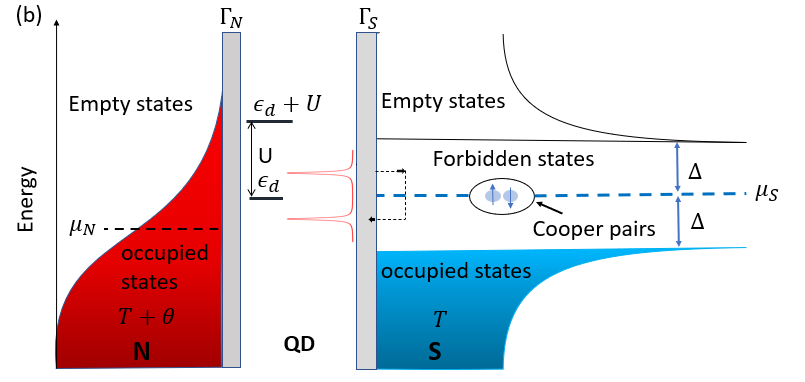
Fig.1(a) illustrates the schematic diagram of the thermoelectric heat engine based on QD. The corresponding band diagram of the N-QD-S system working as a thermoelectric heat engine is shown in Fig.1(b). When a thermal gradient is applied ($T_{N}-T_{S}=\theta$), the electrons flows from the left normal reservoir to the right superconducting reservoir and creates a potential difference $\mu_{N}-\mu_{S}=eV_{th}$, where $V_{th}$ is thermovoltage. The N-QD-S works as a thermoelectric heat engine when the temperature field on the electron motion overcomes the electric field on them, i.e a reverse voltage $\mu_{S}-\mu_{N}=eV$ must be applied.
This paper is organized as follows : A detailed discussion of the model Hamiltonian and theoretical formalism is provided in the preceding section II. The numerical results and discussion for linear and non-linear regime are given in section III. Section IV concludes the present work.

To analyse the thermoelectric transport properties, we describe the N-QD-S system by the following Anderson+BCS model Hamiltonian in second quantization,

$\displaystyle\hat{H}=\hat{H}_{N}+\hat{H}_{S}+\hat{H}_{QD}+\hat{H}_{T}$

(1)

where

		$\displaystyle\hat{H}_{N}=\sum_{k\sigma}(\epsilon_{k,N}c^{\dagger}_{k\sigma,N}c_{k\sigma,N}),$
		$\displaystyle\hat{H}_{S}=\sum_{k\sigma}(\epsilon_{k,S}c^{\dagger}_{k\sigma,S}c_{k\sigma,S})+\sum_{k}\left(\Delta c^{\dagger}_{k\uparrow,S}c^{\dagger}_{-k\downarrow,S}+H.c\right),$
		$\displaystyle\hat{H}_{QD}=\sum_{\sigma}\epsilon_{d}n_{\sigma}+Un_{\uparrow}n_{\downarrow},$
		$\displaystyle\hat{H}_{T}=\sum_{k\sigma,\alpha\in N,S}(V_{k,\alpha}d^{\dagger}_{\sigma}c_{k\sigma\alpha}+{V^{\ast}_{k,\alpha}}c^{\dagger}_{k\sigma,\alpha}d_{\sigma}).$

$\hat{H}_{N}$ describes the normal metallic reservoir in the non-interacting quasi-particle approximation with single electron kinetic energy $\epsilon_{k,N}$ and $c_{k\sigma,N}(c^{\dagger}_{k\sigma,N})$ is the annihilation(creation) operator of an electron with spin $\sigma$ and wave vector $\vec{k}$.
$\hat{H}_{S}$ describes the superconducting reservoir. $c_{k\sigma,S}(c^{\dagger}_{k\sigma,S})$ is the annihilation(creation) operator of an electron with spin $\sigma$, wave vector $\vec{k}$ and energy $\epsilon_{k,S}$. The second term in $\hat{H}_{S}$ describes the BCS pair interaction, with a superconducting energy gap $\Delta$.
$\hat{H}_{QD}$ describes the Hamiltonian for single-level QD with energy $\epsilon_{d}$, and $d_{\sigma}(d^{\dagger}_{\sigma})$ is the annihilation(creation) operator of electron with spin $\sigma$ on the QD and $n_{\sigma}=d_{\sigma}^{\dagger}d_{\sigma}$ is number operator. The QD can have maximum occupancy of two electrons with opposite spins. We also consider the intradot electron-electron Coulomb repulsion with the interaction strength U.
$\hat{H}_{T}$ represents the tunnelling Hamiltonian between the QD energy level and reservoirs with $V_{k\alpha}$ as the tunnelling amplitude between the QD and the $\alpha$-reservoir ($\alpha\in N,S$).
To diagonalized the BCS part of the Hamiltonian, we use Bogoliubov transformation method which defines the new Fermionic quasi-particle operator $\gamma_{k\sigma}(\gamma^{\dagger}_{k\sigma})$ and coefficients $u_{k}$ and $v_{k}$

$\displaystyle c_{k\uparrow,S}=u^{\ast}_{k}\gamma_{k\uparrow}+v_{k}\gamma^{\dagger}_{-k\downarrow},\;\;c^{\dagger}_{-k\downarrow,S}=u_{k}\gamma^{\dagger}_{-k\downarrow}-v^{\ast}_{k}\gamma_{k\uparrow}$

(2)

with normalization condition $|{u_{k}}|^{2}+|{v_{k}}|^{2}=1$. Substituting above equation in Eq.(1) yields following effective model Hamiltonian

	$\displaystyle\hat{H}=$	$\displaystyle\sum_{k,\sigma}(\epsilon_{k,N}c^{\dagger}_{k\sigma,N}c_{k\sigma,N})+\sum_{k\sigma}(V_{k,N}d^{\dagger}_{\sigma}c_{k\sigma,N}+H.c)+$		(3)
		$\displaystyle\sum_{k,\sigma}(E_{k}\gamma^{\dagger}_{k\sigma}\gamma_{k\sigma})+\sum_{k\sigma}(V_{k,S}u^{\ast}_{k}d^{\dagger}_{\sigma}\gamma_{k\sigma}+H.c)+$
		$\displaystyle\sum_{k}[V^{\ast}_{k,S}v_{k}(d^{\dagger}_{\uparrow}\gamma^{\dagger}_{-k\downarrow}-d^{\dagger}_{\downarrow}\gamma^{\dagger}_{k\uparrow})+H.c]+$
		$\displaystyle\sum_{\sigma}\epsilon_{d}n_{\sigma}+Un_{\uparrow}n_{\downarrow}$

where $E_{k}=\sqrt{\epsilon^{2}_{k,S}+|\Delta|^{2}}$ is the excitation quasi-particle energy of the superconducting reservoir. The coefficients $u_{k}$ and $v_{k}$ read

$$|{u_{k}}|^{2}=\frac{1}{2}\left(1+\frac{\epsilon_{k,S}}{\sqrt{{\epsilon^{2}_{k,S}}+|\Delta|^{2}}}\right)$$

(4)

$$|{v_{k}}|^{2}=\frac{1}{2}\left(1-\frac{\epsilon_{k,S}}{\sqrt{{\epsilon^{2}_{k,S}}+|\Delta|^{2}}}\right)$$

(5)

To solve above effective Hamiltonian (Eq.(3)), we use the Green’s function equation of motion method with Zubarev notation Zubarev1960 for the retarded Green’s function $G^{r}_{A,B}(t)={\langle\langle{\hat{A}|\hat{B}}\rangle\rangle}=-i\theta(t)\langle[A(t),B(0)]_{+}\rangle$, where $\hat{A}$ and $\hat{B}$ are creation or annihilation operators, $\theta(t)$ is unit step or heaviside function and $[\hat{A},\hat{B}]_{\pm}=\hat{A}\hat{B}\pm\hat{B}\hat{A}$. The Fourier transform of the above retarded Green’s function ${\langle\langle{\hat{A}|\hat{B}}\rangle\rangle}_{\omega}$ must satisfies the equation of motion (EOM),

$\displaystyle\omega\langle\langle{\hat{A}|\hat{B}}\rangle\rangle_{\omega}=\langle{[\hat{A},\hat{B}]_{+}}\rangle+\langle\langle{[\hat{A},\hat{H}]_{-}|\hat{B}}\rangle\rangle_{\omega}$

(6)

For non-zero Coulomb correlation ($U\neq 0$) an equation of motion for a given Green’s function involves higher-order coupled Green’s functions, thus creating a hierarchy of equations of motion (EOM). In order to truncate the hierarchy of equations one need a decoupling scheme for higher order Green’s functions and maintain self-consistency.
In Nambu representation, we define the retarded Green’s function of the QD as a $2\times 2$ matrices

$${\bf{G}}^{r}_{d}(\omega)={\left\langle\left\langle{\begin{pmatrix}d_{\uparrow}\\ d_{\downarrow}^{\dagger}\\ \end{pmatrix}\begin{pmatrix}d_{\uparrow}^{\dagger}&d_{\downarrow}\end{pmatrix}}\right\rangle\right\rangle}_{\omega}=\begin{pmatrix}\langle\langle{d_{\uparrow}|d_{\uparrow}^{\dagger}}\rangle\rangle_{\omega}&\langle\langle{d_{\uparrow}|d_{\downarrow}}\rangle\rangle_{\omega}\\ \langle\langle{d_{\downarrow}^{\dagger}|d_{\uparrow}^{\dagger}}\rangle\rangle_{\omega}&\langle\langle{d_{\downarrow}^{\dagger}|d_{\downarrow}}\rangle\rangle_{\omega}\\ \end{pmatrix}=\begin{pmatrix}G^{r}_{d,11}(\omega)&G^{r}_{d,12}(\omega)\\ G^{r}_{d,21}(\omega)&G^{r}_{d,22}(\omega)\rangle\rangle\\ \end{pmatrix}$$

(7)

Where the diagonal components of ${\bf{G}}^{r}_{d}(\omega)$ represents the single particle retarded Green’s function of electron with spin $\sigma=\uparrow$ and hole with spin $\sigma=\downarrow$ respectively. The off-diagonal component represents the superconducting paring correlation on the QD.
By evaluating different commutator and anti-commutator brackets we drive the following EOM for the single electron Green’s function with spin $\sigma=\uparrow$

		$\displaystyle(\omega-\epsilon_{d})\langle\langle{d_{\uparrow}|d_{\uparrow}^{\dagger}}\rangle\rangle_{\omega}=1+\sum_{k}V^{\ast}_{k,N}\langle\langle{c_{k\uparrow,N}|d_{\uparrow}^{\dagger}}\rangle\rangle_{\omega}+$		(8)
		$\displaystyle\sum_{k}V_{k,S}u^{\ast}_{k}\langle\langle{\gamma_{k\uparrow}|d_{\uparrow}^{\dagger}}\rangle\rangle_{\omega}+\sum_{k}V_{k,S}v_{k}\langle\langle{\gamma_{-k\downarrow}|d_{\uparrow}^{\dagger}}\rangle\rangle_{\omega}+$
		$\displaystyle U\langle\langle{d_{\uparrow}d_{\downarrow}^{\dagger}d_{\downarrow}|d_{\uparrow}^{\dagger}}\rangle\rangle_{\omega}.$

Similarly, one may write down the equation of motion for other Green’s functions in Eq.(7) and for the relevant correlation functions appearing in those equation of motions.
We treated the Coulomb correlations within Hubbard-I approximation, which correctly describes the Coulomb blockade effectsHubbard1963; Rozhkov2010; Vovchenko2014. It is important to pointed out that in the Hubbard-I decoupling scheme one can manage to retain higher-order tunneling processes through QD as a manifestation of electron-electron interaction, which are missing in the Hartree-Fock approximation based on weak electronic correlation. Within Hubbard-I decoupling scheme EOM for higher order Green’s functions of the form $U\langle\langle{d_{\uparrow}d_{\downarrow}^{\dagger}d_{\downarrow}|d_{\uparrow}^{\dagger}}\rangle\rangle_{\omega}$ is simplified by using,

$$U\langle\langle{c_{k\pm\sigma,N}d_{-\sigma}^{\dagger}d_{-\sigma}|d_{+\sigma}^{\dagger}}\rangle\rangle_{\omega}\rightarrow U\langle n_{-\sigma}\rangle\langle\langle{c_{k\pm\sigma,N}|d_{+\sigma}^{\dagger}}\rangle\rangle_{\omega}$$

(9)

$$U\langle\langle{\gamma_{k\pm\sigma}d_{-\sigma}^{\dagger}d_{-\sigma}|d_{+\sigma}^{\dagger}}\rangle\rangle_{\omega}\rightarrow U\langle n_{-\sigma}\rangle\langle\langle{\gamma_{k\pm\sigma}|d_{+\sigma}^{\dagger}}\rangle\rangle_{\omega}$$

(10)

where $\pm\sigma\in\uparrow,\downarrow$ and $\langle{n_{-\sigma}}\rangle=\langle d_{-\sigma}^{\dagger}d_{-\sigma}\rangle$ denotes the quantum statistical average value of occupation number with spin $-\sigma$.
Within Hubbard-I decoupling scheme the correlations involving reservoir electrons in the higher order Green’s function and the spin flip processes on the dot are neglected (i.e $\langle{d_{-\sigma}^{\dagger}d_{+\sigma}}\rangle$=0). Thus the formalism and results explained in the present paper are relevant for temperatures higher than the temperature associated with the Kondo effect (i.e., Kondo temperature $T_{K}$)Yamada2011. We also assume that the Coulomb correlation effects are manifested only in the diagonal elements of the Green’s function (Eq.(7)) i.e. self-consistent determination of the proximity induced local superconducting gap or pairing amplitude on the QD site is excluded from our analysis (i.e., $\langle d_{\uparrow}d_{\downarrow}\rangle\rightarrow 0$), which drastically reduces the computational time. This assumption is justified in subsection III.D, where we have shown that the inclusion of self-consistent equation for $\langle d_{\uparrow}d_{\downarrow}\rangle$ does not affect the electric and thermoelectric transport properties analysed in the present work.
For simplification the tunnelling amplitude is considered $k$ independent i.e $V_{k,\alpha}=V_{\alpha}$ for $V_{k,\alpha}<<D$ (wide band), where $-D\leq\epsilon_{k,\alpha}\leq D$, with $D$ as the half bandwidth. The tunneling coupling strength of the QD to the $\alpha$-reservoir ($\alpha\in N,S$) is defined by $\Gamma_{\alpha}=2\pi|V_{\alpha}|^{2}\rho_{0,\alpha}$, where normal metallic density of states $\rho_{0,\alpha}$ is constant in the range of energy around Fermi level (flat band). Here $\rho_{0,S}$ is modified in the superconducting state.
Finally after solving coupled EOM based on above Hubbard-I scheme we arrive at the expression for the retarded Green’s function of electron with spin $\sigma=\uparrow$ and off-diagonal superconducting pairing correlation on the QD,

$G_{d,11}^{r}(\omega)=\langle\langle{d_{\uparrow}|d_{\uparrow}^{\dagger}}\rangle\rangle=\cfrac{\left(1+\cfrac{U\langle{n_{\downarrow}}\rangle}{\omega-\epsilon_{d}-U}\right)}{\left[\omega-\epsilon_{d}+\left(\cfrac{i\Gamma_{N}}{2}+\beta(\omega)\right)\left(1+\cfrac{U\langle{n_{\downarrow}}\rangle}{\omega-\epsilon_{d}-U}\right)-\cfrac{\left(1+\cfrac{U\langle{n_{\downarrow}}\rangle}{\omega-\epsilon_{d}-U}\right)\left(1-\cfrac{U\langle{n_{\uparrow}}\rangle}{\omega+\epsilon_{d}+U}\right)\left(\cfrac{\Delta}{|\omega|}\beta(\omega)\right)^{2}}{\omega+\epsilon_{d}+\left(\cfrac{i\Gamma_{N}}{2}+\beta(\omega)\right)\left(1-\cfrac{U\langle{n_{\uparrow}}\rangle}{\omega+\epsilon_{d}+U}\right)}\right]}$

(11)

$$G_{d,21}^{r}(\omega)=\langle\langle{d_{\downarrow}^{\dagger}|d_{\uparrow}^{\dagger}}\rangle\rangle=\left[\cfrac{\left(1-\cfrac{U\langle{n_{\downarrow}}\rangle}{\omega+\epsilon_{d}+U}\right)\left(\cfrac{\Delta}{|\omega|}\beta(\omega)\right)}{\omega+\epsilon_{d}+\left(\cfrac{i\Gamma_{N}}{2}+\beta(\omega)\right)\left(1-\cfrac{U\langle{n_{\downarrow}}\rangle}{\omega+\epsilon_{d}+U}\right)}\right]\times G_{d,11}^{r}(\omega)$$

(12)

with

$$\beta(\omega)=\cfrac{\Gamma_{S}}{2}\rho_{S}(\omega)=\cfrac{\cfrac{\Gamma_{S}}{2}\omega}{\sqrt{\Delta^{2}-\omega^{2}}}\theta(\Delta-|\omega|)+\cfrac{\cfrac{i\Gamma_{S}}{2}|\omega|}{\sqrt{\omega^{2}-\Delta^{2}}}\theta(|\omega|-\Delta)$$

(13)

where $\rho_{S}$ is the modified BCS density of states.
The other matrix elements is given by $G_{d,22}^{r}(\omega)=-G_{d,11}^{r}(-\omega)^{\ast}$ and $G_{d,12}^{r}(\omega)=G_{d,21}^{r}(-\omega)^{\ast}$. These retarded Green’s functions allow us to calculate the advanced and lesser/greater Green’s functions and eventually the single particle thermoelectric properties. The averaged occupation of electrons per spin on the quantum dot ($\langle{n_{\uparrow}}\rangle$=$\langle{n_{\downarrow}}\rangle$ for non-magnetic system) is calculated using the self-consistent integral equation of the form

$$\langle{n_{\sigma}}\rangle=\frac{-i}{2\pi}\int^{\infty}_{-\infty}G^{<}_{d,11}(\omega)d\omega$$

(14)

where the lesser Green’s function $G^{<}_{d}$ is introduced which obeys the Keldysh equation (in the matrix form) Haug2008,

$${\bf{G}}^{<}_{d}(\omega)=-{\bf{G}}^{r}_{d}(\omega){\bf{\Sigma}}^{<}_{d}(\omega){\bf{G}}^{a}_{d}(\omega)$$

(15)

where ${\bf{G}}^{a}_{d}(\omega)=\left[{\bf{G}}^{r}_{d}(\omega)\right]^{\dagger}$ is the advanced Green’s function and ${\bf{\Sigma}}^{<}_{d}(\omega)=-\sum_{\alpha\in N,S}\left[{\bf{\Sigma}}^{r}_{\alpha}-{\bf{\Sigma}}^{a}_{\alpha}\right]{\bf{f}}_{\alpha}(\omega)$ is the lesser self energy matrix given by,

${\bf{\Sigma}}^{<}_{d}(\omega)=\begin{pmatrix}-i\Gamma_{N}f_{N}(\omega-\mu_{N})-\cfrac{i\Gamma_{S}|\omega|}{\sqrt{\omega^{2}-\Delta^{2}}}\theta(|\omega|-\Delta)f_{S}(\omega-\mu_{S})&\cfrac{i\Gamma_{S}\Delta}{\sqrt{\omega^{2}-\Delta^{2}}}\theta(|\omega|-\Delta)f_{S}(\omega-\mu_{S})\\ \cfrac{i\Gamma_{S}\Delta}{\sqrt{\omega^{2}-\Delta^{2}}}\theta(|\omega|-\Delta)f_{S}(\omega-\mu_{S})&-i\Gamma_{N}f_{N}(\omega+\mu_{N})-\cfrac{i\Gamma_{S}|\omega|}{\sqrt{\omega^{2}-\Delta^{2}}}\theta(|\omega|-\Delta)f_{S}(\omega-\mu_{S})\end{pmatrix}$

(16)

Thus the lesser Green’s function for electrons on the QD is given by,

	$\displaystyle G^{<}_{d,11}(\omega)=$	$\displaystyle i\Gamma_{N}f_{N}(\omega-\mu_{N})|G_{d,11}^{r}(\omega)|^{2}+i\Gamma_{N}f_{N}(\omega+\mu_{N})|G_{d,12}^{r}(\omega)|^{2}+$		(17)
		$\displaystyle\cfrac{i\Gamma_{S}|\omega|}{\sqrt{\omega^{2}-\Delta_{2}}}\;\theta(|\omega|-\Delta)f_{S}(\omega-\mu_{S})\left[|G_{d,11}^{r}(\omega)|^{2}+|G_{d,12}^{r}(\omega)|^{2}-\cfrac{2\Delta}{|\omega|}Re\left(G_{d,11}^{r}(\omega).G_{d,12}^{a}(\omega)\right)\right]$

where $\theta(|\omega|-\Delta)$ is the unit step function and $f_{\alpha\in N,S}(\omega\mp\mu_{\alpha})=\left[{exp((\omega\mp\mu_{\alpha})/k_{B}T_{\alpha})+1}\right]^{-1}$ is the Fermi-Dirac distribution function of reservoirs with temperature $T_{\alpha}$ and chemical potential $\pm\mu_{\alpha}$ (measured from Fermi level $\epsilon_{f}$ or $\mu_{f}=0$).
In the linear response regime, i.e., for small Voltage biasing ($\mu_{S}-\mu_{N}=e\delta V\rightarrow 0$) and small temperature gradients ($T_{N}-T_{S}=\delta\theta\rightarrow 0$) between the reservoirs, the Fermi function of the normal and the superconducting reservoirs can be expanded around the equilibrium value (average $T$ with $\mu_{f}=0$), which gives

$$f_{\alpha}(\omega\pm\mu_{\alpha})\approx f_{eq}\pm\cfrac{df_{eq}}{d\omega}\left[\mu_{\alpha}-\left(\cfrac{\omega}{T}\right)(T-T_{\alpha})\right]$$

(18)

where $f_{eq}\!=\!\left[exp(\omega/k_{B}T)+1\right]^{-1}$ is the equilibrium Fermi-Dirac distribution function with $\mu_{S}=\mu_{N}$ and $T_{S}=T_{N}$.
Substituting above linear relation into Eqs.(25)-(30) (given below) gives the electrical current and heat current satisfying the Onsager relationMahan2000,

$$\begin{pmatrix}I_{C}\\ \\ J_{Q}\\ \\ \end{pmatrix}=\begin{pmatrix}e^{2}L_{0}&\cfrac{e}{T}L_{1}\\ \\ eL_{1}&\cfrac{1}{T}L_{2}\\ \end{pmatrix}\\ \begin{pmatrix}\delta V\\ \\ \delta\theta\\ \\ \end{pmatrix}$$

(19)

with thermoelectric response functions

	$\displaystyle L_{0}$	$\displaystyle=\cfrac{2}{h}\int{\left(\cfrac{-df_{eq}}{d\omega}\right)(2T_{A}(\omega)+T_{QP}(\omega))d\omega}$
	$\displaystyle L_{1}$	$\displaystyle=\cfrac{2}{h}\int{\omega\left(\cfrac{-df_{eq}}{d\omega}\right)T_{QP}(\omega)d\omega}$
	$\displaystyle L_{2}$	$\displaystyle=\cfrac{2}{h}\int{\omega^{2}\left(\cfrac{-df_{eq}}{d\omega}\right)T_{QP}(\omega)d\omega}$

Here, $e$ and $h$ denote the magnitude of the electronic charge and Planck’s constant, respectively.

$T_{A}(\omega)=\Gamma_{N}^{2}|G_{d,12}^{r}(\omega)|^{2}$ is the Andreev tunnelling amplitude and $T_{QP}(\omega)=\cfrac{\Gamma_{N}\Gamma_{S}|\omega|}{\sqrt{\omega^{2}-\Delta^{2}}}\;\theta(|\omega|-\Delta)\times\left[|G_{d,11}^{r}(\omega)|^{2}+|G_{d,21}^{r}(\omega)|^{2}-\cfrac{2\Delta}{|\omega|}Re{(G_{d,11}^{r}(\omega)\;G_{d,12}^{a}(\omega))}\right]$ is the quasi-particle tunnelling amplitude.
The thermoelectric transport quantities (electrical conductance $G$, thermopower or Seeback coefficient $S$, and electronic contribution to thermal conductance $K$) are then obtained from Eq.(19).

		$\displaystyle G=\lim_{\delta V\to 0}{\cfrac{I_{C}}{\delta V}}\biggr\rvert_{\delta\theta=0}=e^{2}L_{0}$		(20)
		$\displaystyle S=\lim_{\delta\theta\to 0}{\cfrac{\delta V}{\delta\theta}}\biggr\rvert_{I_{C}=0}=-\cfrac{1}{eT}\frac{L_{1}}{L_{0}}$		(21)
		$\displaystyle K=\lim_{\delta\theta\to 0}{\cfrac{J_{Q}}{\delta\theta}}\biggr\rvert_{I_{C}=0}=\cfrac{1}{T}\left[L_{2}-\cfrac{L_{1}^{2}}{L_{0}}\right]=\cfrac{1}{T}L_{2}-S^{2}GT$		(22)

The electrical conductance is defined as the flow of charge current per unit voltage between the isothermal reservoirs ($\delta\theta=0$). The thermopower (Seebeck coefficient) is defined as the generated voltage per unit thermal gradients in open circuit condition i.e. $I_{C}=0$. The electronic thermal conductance is usually given by the heat flow through the central region (in present case QD) when it is coupled between electrically insulating source and drain reservoirs at different temperatures. In such systems, the reservoirs impose open circuit condition $I_{C}=0$. However, for a thermoelectric system with non-zero $L_{1}$ or $S$, a voltage will build up across the QD proportional to the temperature difference. Thus, total electronic thermal conductance $K$ is reduced as compared to electrically insulating reservoirs by a factor of $S^{2}GT$. Where $P=S^{2}G$ is the corresponding power factor.
The performance of the thermoelectric heat engine in the linear response regime is determined by a dimensionless thermoelectric figure of merit $ZT$.

$$ZT=\cfrac{S^{2}GT}{K}=\cfrac{S^{2}GT}{K_{e}+K_{ph}}$$

(23)

Since we are interested in understanding the electronic thermal properties at low temperatures, we only consider the thermal contribution by electrons, and the lattice or phonon thermal contribution is negligible at low temperatures($K_{e}\approx K$)Hwang2016b; Yang2020.
In the linear response regime, the relationship between figure of merit $ZT$ and efficiency at maximum power output $\eta_{P_{max}}$ is given byErdman2017; Benenti2017

$$\eta_{P_{max}}=\cfrac{\eta_{C}}{2}\;\cfrac{ZT}{ZT+2}$$

(24)

where $\eta_{C}$ is the Carnot efficiency.
In the non-linear regime the system is under the influence of finite voltage biasing $\mu_{N}-\mu_{S}=eV$ (say $\mu_{N}=eV$ and $\mu_{S}=0$) and/or temperature gradient $T_{N}-T_{S}=\theta$ (say $T_{N}=T+\theta$ and $T_{S}=T$). Thus the definition of linear response regime fails, and one needs to go beyond this limit. In the non-equilibrium steady-state condition, the net current flowing through the left normal and right superconducting reservoirs is $I_{N}=-I_{S}\equiv I_{C}$ (current conservation) and can be evaluated from the time evolution of the occupation number operator of the left normal reservoir ($d\langle{-e\sum_{k}c^{\dagger}_{k,N}c_{k,N}}\rangle/dt$)Haug2008; Meir1992.

$$I_{N}\equiv I_{C}=I_{A}+I_{QP};$$

(25)

where

$I_{A}=\cfrac{2e}{h}\int{\left[f_{N}(\omega-\mu_{N})-f_{N}(\omega+\mu_{N})\right]T_{A}(\omega)\;d\omega}$

(26)

$I_{QP}=\cfrac{2e}{h}\int{\left[f_{N}(\omega-\mu_{N})-f_{S}(\omega-\mu_{S})\right]T_{QP}(\omega)\;d\omega}$

(27)

are Andreev and quasi-particle contribution to electrical/charge current respectively.
The heat current is evaluated from the rate of energy flow at the normal reservoir side and Joule heating in the presence of voltage biasing.

$$J_{N}\equiv J_{Q}=\cfrac{-i}{\hbar}\langle{[\hat{H},\hat{H}_{N}]}\rangle-\cfrac{\mu_{N}I_{C}}{e}=J_{A}+J_{QP};$$

(28)

where

$J_{A}=-4\mu_{N}\cfrac{1}{h}\int{\left[f_{N}(\omega-\mu_{N})-f_{N}(\omega+\mu_{N})\right]T_{A}(\omega)\;d\omega=-2\cfrac{\mu_{N}I_{A}}{e}}$

(29)

$J_{QP}=\cfrac{2}{h}\int{(\omega-\mu_{N})\left[f_{N}(\omega-\mu_{N})-f_{S}(\omega-\mu_{S})\right]T_{QP}(\omega)\;d\omega}$

(30)

are Andreev and quasi-particle contribution to heat current respectively. The heat current satisfy the condition $J_{N}+J_{S}=-I_{C}(\mu_{N}-\mu_{S})/e$ and we have shown the calculation for heat current flowing at the normal reservoir side i.e. $J_{Q}\equiv J_{N}=-J_{S}-I_{C}(\mu_{N}-\mu_{S})/e$.
Also, the prefactor 2 in charge and heat current is due to the spin degeneracy. Note that for thermal gradient without voltage biasing (i.e. $\mu_{N}=eV=0$) the subgap ABS heat current is zero and only quasi-particle contributes to the heat current.
In order to use N-QD-S as a heat engine or power generator, the temperature gradient $\theta$ is set larger then zero. Due to this temperature difference electrons move from left reservoir to the right reservoir and thus create a potential difference ($\mu_{N}-\mu_{S}=eV_{th}$) due to accumulation of electrons on the right reservoir and positive charge to the left reservoir.
The thermovoltage ($V_{th}$) thermopower ($S$) and electronic thermal conductance ($K$) is determined from the open circuit condition,

$$I_{C}(V_{th},\theta)=I_{A}(V_{th},\theta)+I_{QP}(V_{th},\theta)=0$$

(31)

For finite Voltage biasing and temperature gradient above equation is solved numerically to obtain $V_{th}$ and eventually $S=\cfrac{V_{th}}{\theta}$ and $K=\cfrac{J_{Q}}{\theta}$.

The heat engine generates a finite power $P$ between $V=0$ and $V=V_{th}$ and is given by,

$$P=-I_{C}V$$

(32)

where $V=(\mu_{S}-\mu_{N})/e$ is bias voltage applied to counteract the thermally induced current i.e power is generated when current is driven against the potential difference.
The thermoelectric efficiency is defined as the ratio between the generated output power (nonlinear current times voltage) and the nonlinear input heat current i.e $\eta=output\;power/input\;heat=P/J_{Q}$. The maximal power generated by the heat engine is calculated numerically by using Eq.(31)&(32) and the relative efficiency at maximal power output is given by,

$$\left(\cfrac{\eta_{P_{max}}}{\eta_{C}}\right)=\cfrac{P_{max}}{J_{Q}}\times{\cfrac{T+\theta}{\theta}}$$

(33)

where Carnot efficiency $\eta_{C}=\cfrac{\theta}{T+\theta}$.

This section presents the numerical results obtained using MATLAB for the linear (subsection III.A) and non-linear response under electric and temperature field in the Coulomb blockade regime. We analyse two different situations in the non-linear transport regime. In the first situation (subsection III.B), we consider a voltage-driven case for isothermal reservoirs ($\theta=0$) and discuss the Andreev and quasi-particle charge and heat transport. In the second situation (subsection III.C), the N-QD-S system is discussed in the context of thermoelectric heat engine for finite $\theta$ and $V$. In our calculations, all energies are expressed in the unit of superconducting energy gap $\Delta$.