Phase-type mixture-of-experts regression for loss severities
Abstract.
The task of modeling claim severities is addressed when data is not consistent with the classical regression assumptions. This framework is common in several lines of business within insurance and reinsurance, where catastrophic losses or heterogeneous sub-populations result in data difficult to model. Their correct analysis is required for pricing insurance products, and some of the most prevalent recent specifications in this direction are mixture-of-experts models. This paper proposes a regression model that generalizes the latter approach to the phase-type distribution setting. More specifically, the concept of mixing is extended to the case where an entire Markov jump process is unobserved and where states can communicate with each other. The covariates then act on the initial probabilities of such underlying chain, which play the role of expert weights. The basic properties of such a model are computed in terms of matrix functionals, and denseness properties are derived, demonstrating their flexibility. An effective estimation procedure is proposed, based on the EM algorithm and multinomial logistic regression, and subsequently illustrated using simulated and real-world datasets. The increased flexibility of the proposed models does not come at a high computational cost, and the motivation and interpretation are equally transparent to simpler MoE models.
1. Introduction
The correct estimation of claim severities is a classical problem in actuarial science, and yet the task remains challenging and often only solvable by partially formal procedures. For instance, when dealing with data arising from reinsurance of natural catastrophes or from third-party liability insurance, very large claims are treated differently to the bulk of smaller – or attritional – claim sizes. Multimodality of the attritional claims can further exacerbate the problem. Such heterogeneity in the data is often still present after segmentation, possibly due to pooled and unlabelled sub-populations in the dataset. In addition, most common commercial software, which mostly uses generalized linear models (GLM), does not capture quantiles correctly. Consequently, risk managers and actuaries interested in understanding their fitted probabilistic models (and not only using them for prediction) keep returning to the drawing board to obtain more interpretable, flexible and effective statistical tools for their practice.
Several statistically coherent approaches have been proposed in recent years to overcome multimodality and heavy-tailedness. For instance, mixing Erlang distributions results in multimodal histograms, Lee and Lin, 2010 being the first to consider such model for insurance, and then later extended by Tzougas et al., 2014; Miljkovic and Grün, 2016 for more general mixtures. More recent approaches, such as Fung et al., 2019, adopt a mixture-of-experts approach, which consists of regressing the component probabilities of a finite mixture model. Regarding the heavy-tailed component, the formal way of dealing with the attritional and large claims jointly has been using splicing – also referred to as composite models – which have a different tail and body distribution (see Grün and Miljkovic, 2019 for a comparison and a good literature review). Combining the two approaches is the state-of-the-art of probabilistic models for loss severity modeling, referred to as composite models. Reynkens et al., 2017 were the first to consider this global approach, and Fung et al., 2021b suggested a feature-selection variant.
The main idea of this paper is to use phase-type (PH) distributions to capture the specificities of heterogeneous data more intuitively and effectively than mixing. The underlying multi-state model is easy to motivate and understand for practitioners and is mathematically convenient for developing their estimation. More specifically, we propose to use PH distributions to describe claim severities and build our regression framework with PH building blocks. PH distributions are defined as the absorption time of a time-homogeneous Markov pure-jump process on a finite state space. In life insurance, such a framework is familiar and understood as the traversing of healthy, disabled, and dead states, with time corresponding to calendar time. In non-life insurance, the states can be regarded as unobserved steps in legal cases or reparations of a building, and time now corresponds to the incurred monetary loss.
Many distributions such as the Erlang, generalized Coxian, and finite mixtures between them are all PH distributions (see Neuts, 1975; Neuts, 1981 for the first systematic approaches, and Bladt and Nielsen, 2017 for a recent comprehensive treatment), and they are even known to be dense in weak convergence on the set of distributions of positive-valued risks (cf. Asmussen, 2008). Most applications of PH were initially in the field of applied probability, but their estimation became widely used after Asmussen et al., 1996 laid out the EM-algorithm for statistical fitting. To correct for non-exponential tail behavior, Albrecher and Bladt, 2019; Albrecher et al., 2022 defined and provided estimation approaches for transformed PH distributions, also known as inhomogeneous phase-type (IPH) laws.
To incorporate rating factors into our model, we consider regressing the initial probabilities of the underlying stochastic process starting in a given state. This is in the same spirit as the mixture-of-experts approaches, cf. Yuksel et al., 2012 for a survey, which can roughly be described as machine learning methods where inhomogeneous data regions are divided into homogeneous ones, where simpler models can suffice for their description. A different approach to regression with PH distributions was considered in Albrecher et al., 2021a; Bladt, 2021, where the proportional intensities (PI) model was proposed. The strength of PH regression models is that no threshold selection is required, and a tail behavior specification can be easily done by choosing an appropriate inhomogeneity function. Moreover, the interaction between the hidden states allows for complex density shapes, going beyond what simple mixing can account for, for a given number of experts. In essence, the latter property can have a parsimonious effect on the number of estimation parameters. However, the phase-type mixture-of-experts (PH-MoE) approach can obtain a wider range of variation for a fixed state-space size than the PI approach and can be faster to estimate for a small number of covariates.
The PH-MoE model is rather flexible, illustrated by two denseness results on: a) multinomial experiments with arbitrary distributions assigned to each outcome; b) more general regression models, subject to some technical conditions. The marginal and conditional distributions associated with the PH-MoE specification fall into the IPH class, for which many closed-form formulas exist, and their tail behavior is well understood. Furthermore, their estimation can be carried out using an ingenious decomposition of the fully observed likelihood into two components: one which may be maximized using a variant of the EM algorithm for PH distributions; and another component can be seen as a weighted one multinomial logistic regression problem.
The remainder of the paper is structured as follows. First, in Section 2, we provide a short reminder of IPH distributions, specify the main regression model, and derive its basic properties, along with the first denseness result. We then prove the denseness of PH-MoE on regression models in Section 3 and provide an effective estimation technique based on the EM algorithm and weighted multinomial regression in Section 4, along with a goodness of fit consideration. In Section 5, we review some common choices of inhomogeneity functions for global fitting and introduce a new alternative to composite splicing models based on piecewise-continuous inhomogeneity functions. Subsequently, we show in Section 6 the practical feasibility of our approach on synthetic and real insurance data. Finally, Section 7 concludes.
2. Phase-type Mixture-of-Experts regression model
2.1. Preliminaries
Let be a time-inhomogeneous Markov pure-jump process on the finite state space , where states are transient and is absorbing. Then, the transition probabilities
can be written in matrix form as
for where is called the intensity matrix, that is, a matrix with negative diagonal elements and non-negative off-diagonal elements such that the rows sum to zero. If we further require that the matrices and commute for every , this can be done by assuming the following structure of the intensity matrix
where is a sub-intensity matrix, is a -dimensional column vector providing the exit rates to the absorbing state, is a -dimensional row vector of zeroes, and is some known positive real function. Since the rows of the intensity matrix sum to zero, the relationship holds, where denotes the -dimensional column vector of ones. In what follows, we always assume this structure of and that the function satisfies for
| (2.1) |
For future reference, we write for the -th canonical basis vector in . Concerning the sub-intensity matrix and the vector of exit rates, we introduce the following notation for their entries
We will make use of functions of matrices in the sequel. The standard unambiguous way of defining them is in terms of the Cauchy formula as follows. Let be any analytic function and a square matrix. Then we define
with a simple path enclosing the eigenvalues of , and is the identity matrix of the same dimension.
Definition 2.1.
Let be an initial distribution on . Then, if , we say that
follows an inhomogeneous phase-type (IPH) distribution and we write .
The density and distribution function of are explicit in terms of functions of matrices and given by
Another attractive property of IPH distributions is that a random variable following this specification can be expressed as the transformation of a phase-type (PH) distributed random variable, that is, the homogenous case corresponding to . More specifically, if , then
| (2.2) |
where and is defined through its inverse in terms of by
This representation is particularly useful to derive further properties of IPH distributions by exploiting the known PH machinery. For instance, the following explicit asymptotic behavior for the tails of IPH distributions can be deduced using this representation in conjunction with the corresponding asymptotic result for PH distribution:
| (2.3) |
where is a positive constant depending on and , is the largest real eigenvalue of , and is the size of the Jordan block associated with .
2.2. The regression model
Define the mapping
where is the standard -simplex. Thus, for any given , we may endow the process with the initial probabilities
and .
As a particular consequence, the following random variable
satisfies that
Definition 2.2.
Let be a -dimensional vector of covariates. Then we say that
is a phase-type mixture-of-experts (PH-MoE) model.
Remark 2.1.
The above model obtains its name since we may write
which is a mixture of PH distributions with different initial distributions, each assigning all its mass to a given state. In particular, we have the simple identity
For instance, in the homogeneous case we obtain
| (2.4) |
Example 2.3.
If is a singleton, then the PH-MoE model exactly spans the class of IPH distributions.
The following result shows that random covariates do not extend the marginal distribution beyond the above example.
Proposition 2.4.
Let be a random vector in a convex . Then the PH-MoE model has marginal distribution given by
for some . In fact, .
Proof.
Let have density . We simply observe that by disintegration we get
and since the process otherwise has the same dynamics after any initiation, the other parameters are unchanged. It remains to notice that by convexity. ∎
For the above reason, the PH-MoE model is most useful in its conditional form, and can be used for regression purposes. We now formulate a particularly advantageous parametrization for when .
Definition 2.5.
We say that the PH-MoE model with initial probabilities given by
| (2.5) |
satisfies the softmax parametrization. Here, , , and .
Remark 2.2.
In essence, we consider the coefficients of as assigning “expertly” each observation to an initial distribution according to their information .
For the above parametrization, we have that the logarithm of the ratio between any two probabilities is linear in that for any ,
However, for two individuals with covariate information and , a class-specific correction arises, as follows:
In regression analyses, in particular, in the analysis of variance (ANOVA) it can often be the case that there is a discrepancy in the mean between observations belonging to two or more categories. However, the conditional distributions may not be Gaussian, or may even be different between different groups. We make a technical definition for such common situations.
Definition 2.6.
Let be positive and continuous random variables having otherwise arbitrary distributions, and let be a multinomial random variable, such that
and such that contains at least an intercept. Then we say that follows a multinomial mixture distribution.
Proposition 2.7.
Let follow a multinomial mixture distribution. Then there exist a sequence of PH-MoE models such that
Moreover, the softmax parametrization may be chosen.
Proof.
We have by definition that for some conditionally independent variables, and a conditionally independent multinomial variable . Given , and by the denseness of PH distributions, there exist sequences of PH distributed random variables , , such that, as ,
Since takes finitely many values, it follows that even
It remains to note that for any given , is a finite mixture of independent PH variables, and thus PH distributed as well, with dimension at most the sum of the individual mixture-component dimensions. Finally, since the covariates contain an intercept term, the softmax function (as a function of )
is a surjective map from to , and we may choose, for each , to exactly match the required initial distribution of . ∎
Remark 2.3.
In the above result, any pre-specified tail behavior of may be exactly matched by all the , by using the appropriate inhomogeneity function . The details are straightforward but technical and thus omitted.
3. Denseness on regression models
This section is devoted to showing a stronger version of Proposition 2.7, under some more restrictive conditions on the covariate space and the associated conditional distributions.
Definition 3.1.
Let be the set of possible values of the covariates . A severity regression model is the set of conditional distributions of claim severity, given the covariates, that is, the set of laws of
Given a severity regression model, we say that a sequence of severity regression models converges weakly (respectively, uniformly weakly) to it, if all the associated conditional distributions converge weakly for each (respectively, uniformly weakly in ).
Definition 3.2.
A feature space is said to be regular if it is of the form , that is, the covariates contain an intercept and are otherwise contained in a hypercube.
Condition 3.3.
A regression model is said to satisfy the tightness and Lipschitz conditions on if
is a tight family of distributions, and for each , the function
is Lipschitz continuous in .
To allow zeroes in the vector of initial probabilities, we can assume without loss of generality that the vector of initial probabilities is of the form , where is a -dimensional column vector, , with
Indeed, we can always reorder the states of the PH representation in such a way that the first entries of are the ones corresponding to the values different from zero.
Proposition 3.4 (Denseness).
Let a regression model satisfy the tightness and Lipschitz conditions on a regular . Then, there exists a sequence of PH-MoE regression models converging uniformly weakly to it.
Proof.
The claim follows from Theorem 3.3 in Fung et al., 2019 by noticing that LRMoE models with Erlang distributed severities (which satisfy Property 3 of Proposition 3.1 in Fung et al., 2019) are particular instances of the PH-MoE model. ∎
Remark 3.1.
Proposition 3.4 also implies that the PH-MoE models, with fixed inhomogeneity transformation , form a dense class on the set of univariate severity regression distributions.
This is relevant since it allows us to obtain different tail behaviors for modeling claim severities. For instance, in Fung et al., 2019, it is shown that Pareto distributions fail to fulfill the denseness conditions in the LRMoE model. This implies that for a fixed splicing threshold, denseness and heavy-tails are not possible in that setting. In contrast, Pareto tail behavior is now possible using a PH-MoE model, while still preserving the denseness property.
It is worth mentioning that another alternative was recently introduced in Fung et al., 2021a, which was termed the TG-LRMoE model. The main idea of this model consists of transforming Gamma distributed random variables to obtain heavy tails for the severity distributions (including Pareto tails). Note, however, that when considering Gamma random variables with integer shape parameters (i.e., Erlang) in the TG-LRMoE specification, we obtain a particular case of a PH-MoE model with intensity , .
4. Estimation
4.1. The EM algorithm
Suppose that we have a PH-MoE specification
By a simple inhomogeneity transformation, we may momentarily concentrate on the homogeneous case as follows:
Now, let be the number of times that the process with initial distribution starts in state , the total number of jumps from state to conditional on , the number of times that we reach the absorbing state from state conditional on , and let be the total time that the underlying Markov jump process spends in state prior to absorption given . Then, given a sample of absorption times and the corresponding paired covariate information , the completely observed likelihood can be written in terms of the previously defined statistics as follows:
with
The above specification partially belongs to the exponential family of distributions and thus has semi-explicit maximum likelihood estimators.
Since the full-trajectory data is not observed, we employ the expectation-maximization (EM) algorithm to estimate part of the MLE iteratively. This implies that at each iteration, the conditional expectations of the sufficient statistics , , , and given the absorption times are computed, corresponding to the E-step. Then is maximized by replacing the values of the statistics by their corresponding expected values from the previous step, obtaining in this way updated parameters , commonly referred to as the M-step.
Then the detailed formulas are given as follows:
- 1)
E-step, conditional expectations:
- 2)
M-step, explicit maximum likelihood estimators:
- 3)
R-step, weighted multinomial regression estimation:
where as before is the standard -simplex.
Finally, to incorporate the inhomogeneity transformation , we assume that this is a parametric function depending on some vector , that is, we consider . Then, is updated in a subsequent step consisting of direct maximization of the incomplete likelihood function with respect to (solely) this parameter.
Remark 4.1.
In general, the set of all functions in the simplex is too broad, and a parametric family is chosen – such as the softmax functions. Even then, no explicit solution for the R-step is available. We describe the entire procedure for the softmax case in Algorithm 1.
In view that the R-step is computed numerically even for the simplest logistic case, we see that Algorithm 1 easily extends to the case where an arbitrary regression model with a categorical response is used to predict the initial Markov probabilities, for instance, when specifying as a neural network. In this framework, the multinomial logistic regression model can be seen as a -layer neural network.
- 1)
Mixture specification: Set
- 2)
Inhomogeneity transformation: Transform the data into
- 3)
E-step: Compute the statistics
- 4)
M-step: Let
- 5)
R-step: Maximize the weighted multinomial logistic regression
and set
- 6)
Inhomogeneity optimization: Maximize
- 7)
Update the current parameters to . Return to step 1 unless a stopping rule is satisfied.
Direct calculations, or general results from EM theory, yield the following result.
Proposition 4.1.
The likelihood function is increasing at each iteration of Algorithm 1. For a given , the likelihood is also bounded, and we guarantee convergence to a (possibly local) maximum.
Notice that although convergence occurs, even if the parameters are such that the MLE of the PH distribution is asymptotically consistent, convergence to such MLE is still not guaranteed.
4.2. Censoring
In applications, an observation may be partially observed, in that only upper and/or lower bounds may be determined, but not its actual size. This incurs in a large bias if the bounds are far apart, and thus a statistical correction is required. Below we outline such adaptation to the estimation technique for PH-MoE models.
In essence, the EM algorithm 1 can be modified to work with censored observations, with just some adjustments on the formulas of the E-step being required. Recall that a data point is said to be right-censored at if it takes an unknown value above , left-censored at if it takes an unknown value below , and more generally interval-censored at if it takes an unknown value within the interval . Moreover, note that for any censored observation of a PH-MoE model , the inhomogeneity transformation results on a censored observation (of the same type) in the homogeneous setting , meaning that we formally only need to deal with the latter case.
In the following, we provide the explicit formulas for the E-step in the interval-censoring setting. Results for left and right censoring then follow as special cases, given that left-censoring can be seen as interval-censoring with and right-censoring is retrieved by fixing and letting . Thus, for a single generic interval-censored observation with covariate information , we have that
The other steps of the algorithm are unchanged.
4.3. Goodness of fit for phase-type regression models
We propose a common visual tool for assessing the goodness of fit of the overall model. The procedure is described for the case when right-censored observations are present since it is the most common scenario in applications. We define the residuals of a PH-MoE model by
which under right-censoring completely at random and assuming (essentially, specifying the null-hypothesis) that the true distribution is indeed such PH-MoE, then by plugging in the estimated parameters from the EM algorithm, we obtain a dataset
which follows a right-censored mean one exponential distribution. Here, , , denote censoring indicators. In turn, we may construct a Kaplan-Meier survival curve for this dataset, , which should roughly resemble . To obtain a confidence band, we may use Greenwood’s formula where is the number of tied values at , and all values yet to be observed (or at risk).
5. Transforms
The shape of the intensity function is a central assumption of the PH-MoE model, which in particular determines the tail behavior, as can be deduced from (2.3). This section introduces two useful global parametrizations for heavy-tailed distributions, and subsequently considers semi-composite models, which combine the conceptual approaches of splicing with our current setting.
Before introducing the parametric forms, we provide the exact tail behavior, which follows immediately from (2.3).
Proposition 5.1.
Let be a PH-MoE specification. Let be the sub-intensity matrix associated with the Markov jump-process restricted to the accessible states when starting according to the distribution . Then
where is a positive constant depending on and , is the largest real eigenvalue of , and is the size of the Jordan block associated with .
In particular, if never has zeros or if all states of the Markov process communicate, then for all , and all subgroups of the population have the same tail parameters.
5.1. Global models
Global models in the context of PH-MoE refer to parametrizations of with respect to the same function on all of , as opposed to piece-wise functions. Such specifications are natural when considering the interpretation of the function: it serves as a time transform that changes throughout time in a smooth way, that is, with continuous derivatives.
Pareto PH-MoE
Consider the transformation
where and . Then, for ,
Here, and . Consequently, the intensity function is given by
We refer to as a Pareto PH-MoE. It then follows from Proposition 5.1 that
as , where is a slowly varying function, that is, it satisfies that for all , and is the largest real eigenvalue of . The Pareto MoE is designed to capture heavy-tailed (in the sense of regular variation) distributions with additional flexibility in the body of the distribution arising from the matrix parameters.
Weibull PH-MoE
If we now instead consider
where and , then for ,
Hence, , , and
We refer to this model as a Weibull PH-MoE, where loosely speaking we obtain, for each observation, a Weibull tail behavior with a matrix in place of the usual scale parameter. From Proposition 5.1, it follows that
| (5.1) |
as , where , , and is as above.
This model is suitable for a wider range of applications, since it falls into the Gumbel max-domain of attraction, which implies that it has strictly lighter tails than those of Pareto-type. However, for (respectively, ), we get that (5.1) specifies heavier (respectively, lighter) tails than exponentially decaying ones.
An interesting feature of this specification, and contrary to the Pareto case, is that conditional means are fully explicit and given by
Example 5.2 (Different tail behaviors).
We illustrate the importance of Proposition 5.1 by providing a simple two-groups case where different tail behavior arises. Consider the matrix
and two groups with initial distributions
respectively. Then the first group can only access the first two states, and thus its tail is of the order (since is the largest eigenvalue of the sub-matrix ), while the second group can only access the third state, and thus has a tail of order .
Similarly, if a Pareto inhomogeneity function is used, the tail index will vary between the two groups. Thus, after estimation, it is important to check which states are accessible by which sub-populations, in order to deduce their precise conditional tail asymptotics.
5.2. Semi-composite models as an alternative to splicing
When heavy tails are present, a standard approach to obtain a global model for claim severities is to model the body and tail separately, and then combine them through splicing or mixing. For describing the tail of the distribution, extreme value tools are typically employed. Although this two-step procedure is not fully satisfactory, the outcome can be more reliable when the parameter of interest is the tail coefficient, see, for instance, Embrechts et al., 2013.
On the other hand, the models presented in the previous section are attractive alternatives to obtain global models, due to their authentic heavy tails and denseness. Moreover, the fitting of these models does not require any form of threshold selection, as in traditional extreme value techniques. However, their estimation methods give the same weight to all data points, and hence the automatic modeling of the tails may not be as satisfactory as when targeting the tail via thresholding. Furthermore, in some situations, even if the tail is correctly specified via fitting a PH-MoE model using the EM algorithm, a risk manager might be interested in at least partially separating the analysis above and below a certain threshold.
Below we see how certain piecewise specifications for the inhomogeneity function can achieve a compromise between the two above approaches, while still formally falling into the class of standard PH-MoE models. Specifically, we consider inhomogeneity transformations which are defined differently below and above a certain threshold (and the idea can be extended to several layers).
Definition 5.3.
We say that a PH-MoE model is semi-composite if its intensity function is of the form
for any two intensities .
An immediate consequence is the following:
Proposition 5.4.
For a semi-composite PH-MoE model we have that
and so in particular
Hence, is tail-equivalent to a PH-MoE model with intensity for all .
Below we outline the details of two cases which give rise to tails which are commonly used for loss modeling.
Example 5.5 (PH body with Weibull tail).
Specify
In this way
and
Hence
Example 5.6 (PH body with Pareto tail).
We may instead specify
Which now yields
and
Hence
Note that for fix , the proposed models are dense in the class of distributions in the positive real line. This follows from the fact that they belong to the IPH class, which possesses the said property for any satisfying (2.1).
Given that the intensity function is a parametric function depending on the parameters and , we can employ Algorithm 1 for the estimation of the above semi-composite specifications. However, the changepoint may alternatively be specified in advance and then fixed through the fitting procedure. The latter approach is preferable in almost all cases, and in particular when working with regularly-varying heavy tails, where the threshold may be determined by well-founded visual tools, such as the Hill estimator, cf. Hill, 1975.
6. Numerical examples
This section illustrates the statistical feasibility of the methods developed above. We do not aim to be comprehensive in our treatment, but instead point out the general direction which seems promising. The drawback of the algorithm at the moment is speed, in particular of the R-step, which is a well-known issue of multinomial regression models when in the presence of several covariates. Hence, we provide one simulated example with a -dimensional categorical covariate, and a much larger real insurance example with two categorical covariates.
6.1. Synthetic data
We consider a simulated example where the data genuinely comes from a classical mixture-of-experts model. More precisely, the dataset consists of a total of observations divided into groups of size , each having distributions as follows:
We consider a -dimensional PH structure, which was chosen small enough so that if there were no interaction between states, it would not be possible to model the four groups. Indeed, mixtures of five exponential components would not correctly capture the four given distributions.
Subsequently, we employed a homogeneous version of Algorithm 1, where Steps 2 and 6 are suppressed. In other words, we assume that , , and in particular, the tails of both the data and the model are exponentially decaying. The results are as follows11 1 Here and in the rest of the numerical section, estimates are rounded to three decimal places. This means that some displayed null values may actually be very small but non-zero.:
and the output of the R-step is given in Table 6.1.
| State | (Intercept) | Group B | Group C | Group D |
|---|---|---|---|---|
| 2 | -9.986 (6.673) | 17.488 (24.118) | 8.732 (6.675) | 13.983 (30.537) |
| 3 | -4.32 (0.395) | -3.113 (0.044) | 4.308 (0.41) | 17.281 (29.532) |
| 4 | -12.642 (25.17) | 25.136 (34.211) | 12.002 (25.17) | 8.02 (300.3) |
| 5 | -4.488 (0.429) | 6 (25.6) | 3.079 (0.464) | 13.74 (29.534) |
In particular, the coefficients translate into the following initial Markov probabilities for each group:
When considering the means for each group, given by formula (2.4), we obtain, upon comparing with a Gamma Generalized Linear Model (GLM), the following table:
| Group | Theoretical | Empirical (GLM) | PH-MoE |
|---|---|---|---|
| A | 3 | 3.005 | 3.021 |
| B | 27 | 27.212 | 26.347 |
| C | 9 | 9.463 | 10.001 |
| D | 9 | 9.499 | 9.807 |
Since the PH-MoE does not match the empirical means for each group, as is the case for the GLM, we can observe slight discrepancies between the fitted and observed averages per group. However, if we estimate the dispersion coefficient of the GLM with the average deviance, we may compare not only the mean but the entire distribution of both models. Figure 6.1 shows the densities for each group for the theoretical and fitted cases, and for the GLM and PH-MoE models. We observe that the risks are better understood if we use the latter model, and consequently, any other measure of performance which is not solely based on the mean will favor the matrix-based method.


6.2. Insurance data
We consider the French Motor Third Party Liability (freMTPL) insurance data, contained in the datasets freMTPLfreq and freMTPLsev in the CASdatasets package in R. The data consists of risk features corresponding to motor insurance policies and the number of claims and their severity. Presently we aim at analyzing only a portion of the total claim sizes22 2 Here, we have divided claim severities by the corresponding claim numbers for each policy. For numerical reasons, we also divided the result by ., mainly for computational power reasons: the multinomial step of the PH-MoE routine can be slow to (or not) converge for large (say, above ), (in the tens of thousands) and (more than covariates).
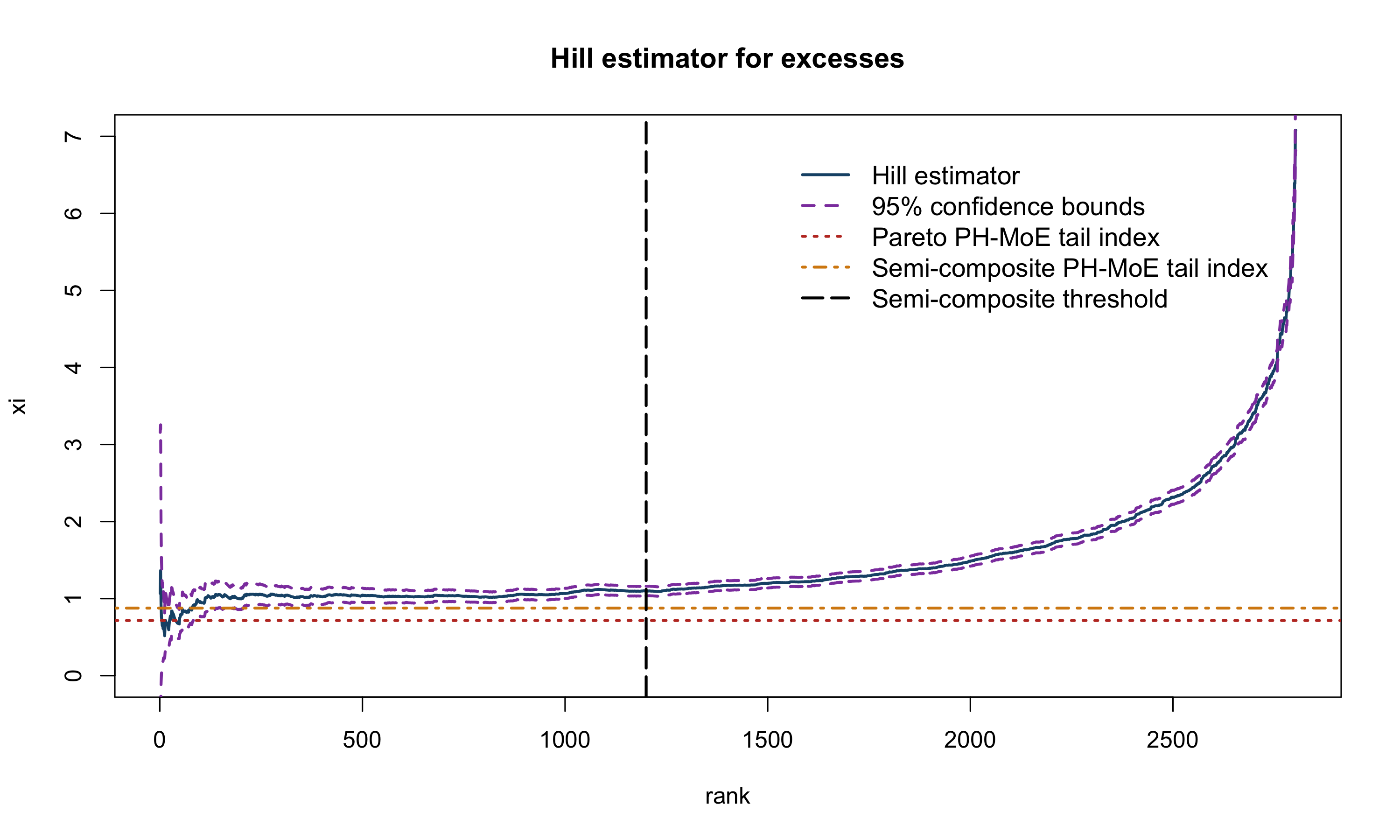
To find a sensible and interesting subset of the data, we first observe the top left panel of Figure 6.2, where we see that the data has a highly pronounced peak in the log scale. Such peak can only be captured by a PH distribution of a huge order (), which makes it unfeasible to fit even without covariates. Thus, we consider only the excesses above the threshold , which in insurance terms would correspond to data entering an XL reinsurance contract with retention level . The excesses are plotted in the top right panel of Figure 6.2 in the log scale, which are much easier to estimate with a lower dimension. On the bottom panel of Figure 6.2, we observe the heavy-tailed nature of the excesses and that there is a substantial bias away from strict Pareto behavior (the estimator curves for smaller order statistics).


With respect to covariates, we fitted a log-normal regression model and selected the only two covariates which seem to be relevant to predicting the mean33 3 In general, insurance covariates provide very small predictive power for severity, in contrast to claim counts, where the performance is usually much better. :
- (1)
Power: The power of the car, an ordered categorical variable with values: d, e, f, g, h, i, j, k, l, m, n, o.
- (2)
Region: The policy region in France, based on the 1970-2015 classification. Possible values associated with the excesses are: Aquitaine, Basse-Normandie, Bretagne, Centre, Haute-Normandie, Ile-de-France, Limousin, Nord-Pas-de-Calais Pays-de-la-Loire, Poitou-Charentes.
To illustrate and compare the modeling capabilities of our model, we proceed to estimate different PH-MoE and LRMoE models, the latter being a natural candidate for comparison. More specifically, and to keep the number of parameters for both models similar, we considered three Pareto PH-MoE models of dimensions 3, 4, and 5, and three LRMoE models with 4, 5, and 6 experts. For the PH-MoE models, we employed EM steps with random initialization of the parameters. On the other hand, the estimation of the LRMoE models was done using the LRMoE R package (cf. Tseung et al., 2020) and as per the Vignettes found in https://github.com/UofTActuarial/LRMoE/tree/master/vignettes with CEM steps and expert components automatically chosen with the cmm_init function. A summary of the results can be found in Table 6.3 and Table 6.4.
| PH-MoE | |||
| Dimension | |||
| Log Likelihood | |||
| Number of parameters | |||
| Computational times | 3.14 mins | 6.24 mins | 11.88 mins |
| LRMoE | |||
| Number Experts | |||
| Log Likelihood | |||
| Number of parameters | |||
| Computational times | 49.75 mins | 1.21 hours | 1.65 hours |
Although perhaps mathematically more complex, our investigations show that the numerical routines for PH-MoE models are at least on par with those of LRMoE in terms of likelihood performance, and certainly much faster. Note also that the number of EM steps cannot be compared with those of the CEM algorithm since the latter is much slower but converges in fewer iterations. This is in line with the thinking of the additional parameters of a PH-MoE model as weak learners rather than actual statistical parameters. A full systematic comparison between PH-MoE, LRMoE, TG-LRMoE, and related MoE models in terms of in-sample and out-of-sample performance is out of the scope of this work. However, we can mention that an advantage of having better computational times, is that we can try different initializations for the EM algorithm. This is highly relevant for the estimation of both models since there is always the possibility of obtaining a local maxima depending on the initial values.
It can be appreciated that the number of parameters involved in both models is relatively large. However, it is crucial to understand that these models can be considered as interpretable machine learning methods rather than concise statistical models. In other words, each additional degree of freedom does not always target a particular distributional feature but instead serves as a weak learner, working towards an overall good estimation. Hence, classical information criteria such as AIC and BIC will tend to overpenalize these models and should not be used for model selection. Ideally, an information criterion specifically designed for PH-MoE models (and even for PH variables) would allow for goodness of fit considerations without using the misspecified AIC and BIC criteria, similar to the development of AICC in the context of time series analysis. Regularization through cross-validation is also a natural topic of further study, but out of the scope of the current manuscript.
With the different PH-MoE models above at hand, we now select one to describe our data and present the results. We start by giving some words about the dimension selection of the PH-MoE model, for which we will follow the typical approach of dimension selection for PH distributions. More specifically, given that adding more dimensions always improves the quality of the fit, one typically starts with low dimensions and assesses the benefit/cost of adding extra dimensions. This assessment is usually done using visual aids and/or by looking at changes in the loglikelihood. One aims for a dimension that is a good compromise between the quality of the fit and a reasonable number of parameters. The reason for this approach is the identifiability issues of PH distribution, meaning that the number of free parameters is unknown. However, it is worth mentioning that recent steps towards more statistical-based selection approaches have been recently introduced in the literature. For instance, we can mention the work in Albrecher et al., 2021b.
In our particular case of study, dimension 5 seems to be a good compromise. To support our choice, we also fitted a PH-MoE model of dimension 6, obtaining an increase in the loglikelihood of , and additional 32 parameters, which was a much smaller likelihood increase than the previous steps. Hence, we decided to stick to a PH-MoE of dimension 5. For completeness, we also fitted a semi-composite PH-MoE with Pareto tail and same dimension 5. In this case, we select the threshold value to be at the order statistic number , which is when the Hill plot visually starts to flatten, obtaining a loglikelihood of . It is worth mentioning that we are selecting the threshold but not the implied tail index. The latter is estimated during the EM algorithm jointly with all other parameters.
The full fitted coefficients and their statistical significance are given in Appendix A, with the asymptotic properties of the MLE delegated to Appendix B. In Figure 6.3, we observe that the densities shift their shapes when varying the covariates, as expected. The semi-composite model has a discontinuity at , which is slightly visible, a feature that is also common in fully composite models. The associated PH-MoE probabilities for these two densities are as follows:
| Pareto PH-MoE: | |||
| S-C PH-MoE: | |||


Note that all the five states in both cases communicate, then the resulting tail indices for the PH-MoE models are given by
which, according to the lower panel of Figure 6.2, are both very reasonable estimates. Further evidence of the quality of the estimation is given in Figure 6.4, where we observe that the empirical distribution function of the residuals of PH-MoE models (computed as described in Section 4.3) align closely with the distribution function of a standard exponential. This is further supported by applying Kolmogorov-Smirnov tests, for which we obtain a p-value of for the PH-MoE and for the semi-composite PH-MoE. Figure 6.5 shows how the intensity functions behave, which may be considered as an infinitesimal “environment” time change of the underlying phase-type distribution. Another possible extension of our model is to make these transformations dependent on .


To extend the analysis to the full data and not only excesses, a direction which is promising is to consider special sub-structures of phase-type distributions. In those cases, the EM algorithm becomes simpler and potentially much faster, consequently enabling the analysis of larger models with more phases being fitted to larger data.
7. Conclusion
We have presented a claim severities regression model based on PH distributions, incorporating covariates through the initial probability vector, which can be cast into a mixture-of-experts framework. When combined with an inhomogeneity transform, these regression models span distributions with different tail behaviors and possible multimodality. Furthermore, they are flexible and may converge to fairly general regression model specifications. We have derived an effective estimation procedure based on the EM algorithm and a weighted multinomial regression problem and shown its feasibility on synthetic and real insurance data.
Several questions remain open for further research, such as automatic feature selection procedures or using other machine learning methods to predict the initial probability vector. In addition, the analysis of more than one risk, together with their respective claim frequencies, all together in a global model with the same underlying Markov structure is an interesting research direction.
Acknowledgement. MB would like to acknowledge financial support from the Swiss National Science Foundation Project 200021_191984. JY would like to acknowledge financial support from the Swiss National Science Foundation Project IZHRZ0_180549.
Declaration MB and JY declare no conflict of interest related to the current manuscript.
Appendix A Estimated coefficients for the PH-MoE models
| State:VariableLevel | Pareto PH-MoE | Semi-composite PH-MoE |
| 2:(Intercept) | ||
| 2:Powere | ||
| 2:Powerf | ||
| 2:Powerg | ||
| 2:Powerh | ||
| 2:Poweri | ||
| 2:Powerj | ||
| 2:Powerk | ||
| 2:Powerl | ||
| 2:Powerm | ||
| 2:Powern | ||
| 2:Powero | ||
| 2:RegionBasse-Normandie | ||
| 2:RegionBretagne | ||
| 2:RegionCentre | ||
| 2:RegionHaute-Normandie | ||
| 2:RegionIle-de-France | ||
| 2:RegionLimousin | ||
| 2:RegionNord-Pas-de-Calais | ||
| 2:RegionPays-de-la-Loire | ||
| 2:RegionPoitou-Charentes | ||
| 3:(Intercept) | ||
| 3:Powere | ||
| 3:Powerf | ||
| 3:Powerg | ||
| 3:Powerh | ||
| 3:Poweri | ||
| 3:Powerj | ||
| 3:Powerk | ||
| 3:Powerl | ||
| 3:Powerm | ||
| 3:Powern | ||
| 3:Powero | ||
| 3:RegionBasse-Normandie | ||
| 3:RegionBretagne | ||
| 3:RegionCentre | ||
| 3:RegionHaute-Normandie | ||
| 3:RegionIle-de-France | ||
| 3:RegionLimousin | ||
| 3:RegionNord-Pas-de-Calais | ||
| 3:RegionPays-de-la-Loire | ||
| 3:RegionPoitou-Charentes | ||
| 4:(Intercept) | ||
| 4:Powere | ||
| 4:Powerf | ||
| 4:Powerg | ||
| 4:Powerh | ||
| 4:Poweri | ||
| 4:Powerj | ||
| 4:Powerk | ||
| 4:Powerl | ||
| 4:Powerm | ||
| 4:Powern | ||
| 4:Powero | ||
| 4:RegionBasse-Normandie | ||
| 4:RegionBretagne | ||
| 4:RegionCentre | ||
| 4:RegionHaute-Normandie | ||
| 4:RegionIle-de-France | ||
| 4:RegionLimousin | ||
| 4:RegionNord-Pas-de-Calais | ||
| 4:RegionPays-de-la-Loire | ||
| 4:RegionPoitou-Charentes | ||
| 5:(Intercept) | ||
| 5:Powere | ||
| 5:Powerf | ||
| 5:Powerg | ||
| 5:Powerh | ||
| 5:Poweri | ||
| 5:Powerj | ||
| 5:Powerk | ||
| 5:Powerl | ||
| 5:Powerm | ||
| 5:Powern | ||
| 5:Powero | ||
| 5:RegionBasse-Normandie | ||
| 5:RegionBretagne | ||
| 5:RegionCentre | ||
| 5:RegionHaute-Normandie | ||
| 5:RegionIle-de-France | ||
| 5:RegionLimousin | ||
| 5:RegionNord-Pas-de-Calais | ||
| 5:RegionPays-de-la-Loire | ||
| 5:RegionPoitou-Charentes |
Appendix B Inference for phase-type regression models
Inference and goodness of fit can always be done via parametric bootstrap methods. However, re-fitting a PH regression can be too costly. A first approach is the following general-purpose result:
Theorem B.1.
Let , be such that the log-density
satisfies Assumptions A0)-A3) of Section 6.3 of Lehmann and Casella, 2006 (common supports, identifiable parameters, i.i.d. observations, and true parameters in the interior of the parameter space) and Assumptions A)-D) of Section 6.5 of Lehmann and Casella, 2006 (existence and finite expectation of third derivatives of log-density, strict positive-definiteness of information matrix, and the representation of the latter in terms of expected double partial derivatives of the log-density).
Then, as the sample size , we have that
- (1)
There exist consistent solutions to the likelihood equations.
- (2)
The following convergence holds:
where is the information matrix.
- (3)
The -th parameter is asymptotically efficient:
Proof.
The proof translates directly from Theorem in Section of Lehmann and Casella, 2006. ∎
Theorem B.1 is somewhat academic in nature for general PH distributions, because although most of the properties are easy to verify for most parameters and transforms, others are difficult, such as the moment conditions, or near-impossible, such as the identifiability and strict positive-definiteness of the information matrix. Indeed, the latter conditions require that all eigenvalues of be distinct (although this is not sufficient) and that all parameters be away from the border regions, which is an uncommon scenario when fitting real data.
However, there is still something to be said when it comes to the regression coefficients. Once the EM algorithm has converged, we may consider the parameters as nuisance parameters and thus perform inference on the partial likelihood , cf. Cox, 1975, see also Wong, 1986. As the latter reference suggests, the sub-optimal use of information incurs a loss of efficiency (standard errors should be considered only as lower bounds) which should be weighted against the possible gains in robustness and simplicity of analysis. The usual experiments where the partial likelihood is useful is when the nuisance parameters take values in high-dimensional spaces, making the calculation of the matrix difficult and not robust. Since the number of nuisance parameters for a PH-MoE model is at least , it is a clear candidate for benefitting from these tradeoffs.
Another advantage of performing inference on the regression variables alone is that we circumvent making allusion to the possibly non-identifiable parameters of the sub-intensity matrix . In practice, this means that we perform inference during the multinomial regression step (R-step) of Algorithm 1, and use the output to draw conclusions on the statistical significance of the covariates , as well as to perform variable selection.
References
- Albrecher and Bladt, (2019) Albrecher, H. and Bladt, M. (2019). Inhomogeneous phase-type distributions and heavy tails. Journal of Applied Probability, 56(4):1044–1064.
- (2) Albrecher, H., Bladt, M., Bladt, M., and Yslas, J. (2021a). Mortality modeling and regression with matrix distributions. arXiv:2011.03219.
- (3) Albrecher, H., Bladt, M., and Muller, L. J. (2021b). Penalised likelihood methods for phase-type dimension selection. Preprint.
- Albrecher et al., (2022) Albrecher, H., Bladt, M., and Yslas, J. (2022). Fitting inhomogeneous phase-type distributions to data: The univariate and the multivariate case. Scandinavian Journal of Statistics, 49(1):44–77.
- Asmussen, (2008) Asmussen, S. (2008). Applied Probability and Queues, volume 51. Springer Science & Business Media.
- Asmussen et al., (1996) Asmussen, S., Nerman, O., and Olsson, M. (1996). Fitting phase-type distributions via the EM algorithm. Scandinavian Journal of Statistics, 23(4):419–441.
- Bladt, (2021) Bladt, M. (2021). Phase-type distributions for claim severity regression modeling. ASTIN Bulletin: The Journal of the IAA, pages 1–32.
- Bladt and Nielsen, (2017) Bladt, M. and Nielsen, B. F. (2017). Matrix-Exponential Distributions in Applied Probability. Springer.
- Cox, (1975) Cox, D. R. (1975). Partial likelihood. Biometrika, 62(2):269–276.
- Embrechts et al., (2013) Embrechts, P., Klüppelberg, C., and Mikosch, T. (2013). Modelling Extremal Events: For Insurance and Finance, volume 33. Springer Science & Business Media.
- Fung et al., (2019) Fung, T. C., Badescu, A. L., and Lin, X. S. (2019). A class of mixture of experts models for general insurance: Theoretical developments. Insurance: Mathematics and Economics, 89:111–127.
- (12) Fung, T. C., Badescu, A. L., and Lin, X. S. (2021a). A new class of severity regression models with an application to IBNR prediction. North American Actuarial Journal, 25(2):206–231.
- (13) Fung, T. C., Tzougas, G., and Wuthrich, M. (2021b). Mixture composite regression models with multi-type feature selection. arXiv:2103.07200.
- Grün and Miljkovic, (2019) Grün, B. and Miljkovic, T. (2019). Extending composite loss models using a general framework of advanced computational tools. Scandinavian Actuarial Journal, 2019(8):642–660.
- Hill, (1975) Hill, B. M. (1975). A simple general approach to inference about the tail of a distribution. The Annals of Statistics, 3(5):1163–1174.
- Lee and Lin, (2010) Lee, S. C. and Lin, X. S. (2010). Modeling and evaluating insurance losses via mixtures of Erlang distributions. North American Actuarial Journal, 14(1):107–130.
- Lehmann and Casella, (2006) Lehmann, E. L. and Casella, G. (2006). Theory of Point Estimation. Springer Science & Business Media.
- Miljkovic and Grün, (2016) Miljkovic, T. and Grün, B. (2016). Modeling loss data using mixtures of distributions. Insurance: Mathematics and Economics, 70:387–396.
- Neuts, (1975) Neuts, M. F. (1975). Probability distributions of phase type. In Liber Amicorum Professor Emeritus H. Florin, pages 173–206. Department of Mathematics, University of Louvian, Belgium.
- Neuts, (1981) Neuts, M. F. (1981). Matrix-geometric solutions in stochastic models, volume 2 of Johns Hopkins Series in the Mathematical Sciences.
- Reynkens et al., (2017) Reynkens, T., Verbelen, R., Beirlant, J., and Antonio, K. (2017). Modelling censored losses using splicing: A global fit strategy with mixed Erlang and extreme value distributions. Insurance: Mathematics and Economics, 77:65–77.
- Tseung et al., (2020) Tseung, S. C., Badescu, A., Fung, T. C., and Lin, X. S. (2020). LRMoE: an R package for flexible actuarial loss modelling using mixture of experts regression model. Available at SSRN 3740215.
- Tzougas et al., (2014) Tzougas, G., Vrontos, S., and Frangos, N. (2014). Optimal bonus-malus systems using finite mixture models. ASTIN Bulletin: The Journal of the IAA, 44(2):417–444.
- Wong, (1986) Wong, W. H. (1986). Theory of partial likelihood. The Annals of Statistics, 14(1):88–123.
- Yuksel et al., (2012) Yuksel, S. E., Wilson, J. N., and Gader, P. D. (2012). Twenty years of mixture of experts. IEEE Transactions on Neural Networks and Learning Systems, 23(8):1177–1193.