Bunch Shaping in Electron Linear AcceleratorsPreprint: APS/123-QED

We consider the motion of a charged particle under electromagnetic field $\mathbf{E}$ and $\mathbf{B}$ satisfying Maxwell equations:

	$\displaystyle\nabla\cdot\mathbf{E}$	$\displaystyle=$	$\displaystyle\frac{1}{\varepsilon_{0}}\rho_{S},$
	$\displaystyle\nabla\cdot\mathbf{B}$	$\displaystyle=$	$\displaystyle 0,$
	$\displaystyle\nabla\times\mathbf{E}$	$\displaystyle=$	$\displaystyle-\frac{\partial}{\partial t}\mathbf{B},$
	$\displaystyle\nabla\times\mathbf{B}$	$\displaystyle=$	$\displaystyle\mu_{0}\mathbf{J}_{S}+\frac{1}{c^{2}}\frac{\partial}{\partial t}\mathbf{E}$		(1)

Here $\rho_{S}$ and $\mathbf{J}_{S}$ are the charge density and current density of the sources, respectively, consisting of the external sources and the beam itself. External sources are not present within the beam pipes. Thus $\rho_{S}=0$ and $\mathbf{J}_{S}=0$ until we consider the beam generated fields in II.4. We will use the MKS units throughout this paper. Introducing the vector and the scalar potential, $\mathbf{A}$ and $\phi$ , respectively, the electromagnetic fields can be written as follows:

$$\mathbf{B}=\mathbf{\nabla}\times\mathbf{A}\mbox{\penalty\ and\penalty\ }\mathbf{E}=-\frac{\partial}{\partial t}\mathbf{A}-\mathbf{\nabla}\phi.$$

(2)

The Hamiltonian $H$ for a particle of mass $m$ and charge $e$ is

$$H(\mathbf{x},\mathbf{p},t)=\sqrt{m^{2}c^{4}+c^{2}(\mathbf{p}-e\mathbf{A}(\mathbf{x},t))^{2}}+e\phi(\mathbf{x},t).$$

(3)

Here $c$ is the velocity of light, $\mathbf{x}$ the coordinate vector, and $\mathbf{p}$ is the canonical momentum conjugate to $\mathbf{x}$.

The Hamiltonian equations of motion are

	$\displaystyle\frac{d\mathbf{x}}{dt}$	$\displaystyle=$	$\displaystyle\frac{\partial H}{\partial\mathbf{p}},$
	$\displaystyle\frac{d\mathbf{p}}{dt}$	$\displaystyle=$	$\displaystyle-\frac{\partial H}{\partial\mathbf{x}}.$		(4)

The Hamilton’s equations reproduce the Lorentz force equation:

$$\frac{d{\mathbf{p}}_{kin}}{dt}=e\left(\mathbf{E}+\mathbf{v}\times\mathbf{B}\right).$$

(5)

Here, $\mathbf{p}_{kin}$ is the kinetic momentum related to the canonical momentum $\mathbf{p}$ as follows:

$$\mathbf{p}_{kin}\equiv m\gamma\frac{d\mathbf{x}}{dt}=\mathbf{p}-e\mathbf{A},$$

(6)

where $\gamma$ = relativistic kinetic energy$/mc^{2}=1/\sqrt{1-\beta^{2}}$, $\beta=v/c$, $v=|d\mathbf{x}/dt|$.

In a beam, particles are bunched in a small region of space and stay together while moving. Therefore, it makes sense to introduce a “reference” particle as the one that is at the beam “center”. Its trajectory is referred to as the reference orbit, which may be curved but will be assumed to lie on a plane referred to as the horizontal plane. The reference orbit is parametrized as $\mathbf{x}_{0}(s)$ where $s$ is the arc length along the reference orbit. Then the position of any particle in the beam can be represented as:

$$\mathbf{x}=\mathbf{x}_{0}(s)+x\mathbf{e}_{\rho}+y\mathbf{e}_{y},$$

(7)

where $\mathbf{e}_{\rho}$ is the unit vector normal to the reference orbit at $s$ on the horizontal plane and $\mathbf{e}_{y}$ is the unit vector normal in the vertical direction. The set $(x,y,s)$ constitutes the curvilinear coordinate system shown in Fig. 2. The figure is drawn on the horizontal plane on which the reference trajectory $\mathbf{x}_{0}(s)$ (solid line) lies. The unit vector $\mathbf{e}_{\rho}$ is in the horizontal plane and perpendicular to the reference trajectory and the unit vector $\mathbf{e}_{y}$ is directed towards the reader. The line perpendicular to the reference trajectory at $s$ represents the transverse plane extending in the vertical direction. The dotted line represents the projection in the horizontal plane of an arbitrary particle, intersecting the transverse plane at $s$ at $(x,y)$.

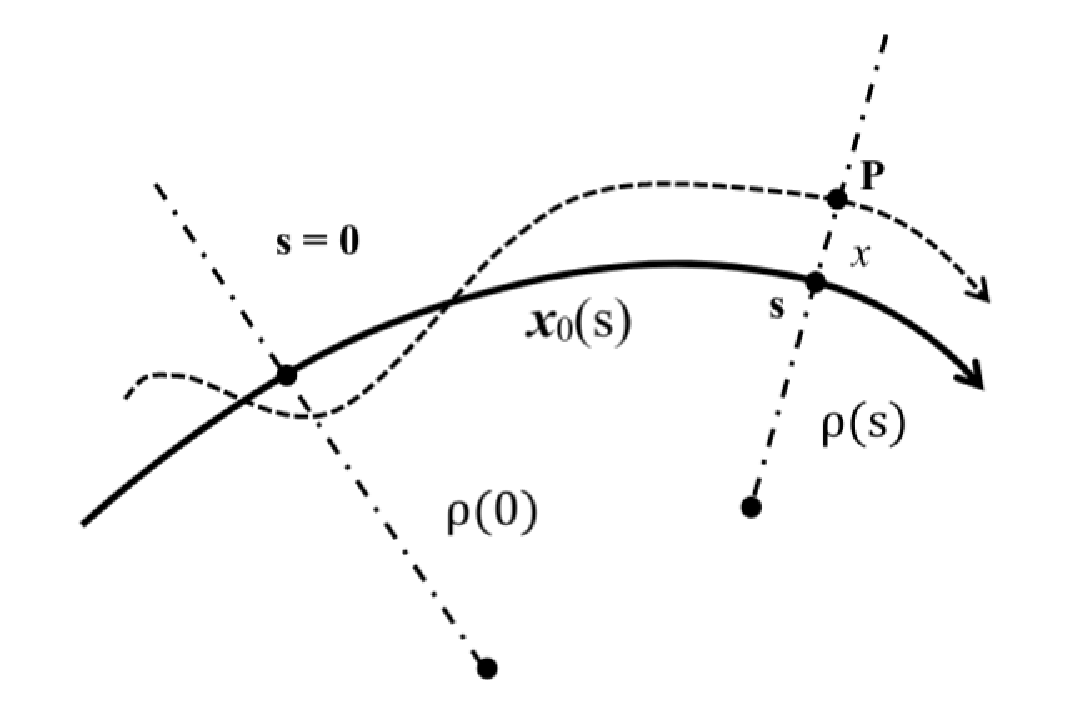
We now make two canonical transformations Landau and Lifshitz 1969; Goldstein 2002 to change the variables to ones convenient for studying beams in accelerators: First, we adopt $s$ as the independent variable and use $(x,y,-t)$ as the coordinates Courant and Snyder 1958, where $t$ is the time the particle arrives at the transverse plane at $s$. The new canonically conjugate variables are:

$$\mathbf{x}_{new}=(x,y,-t),\;\mathbf{p}_{new}=\left(p_{x},p_{y},U\right),$$

(8)

where $U$ is the energy of the particle The new Hamiltonian is ;

$${\mathcal{H}}\left(\mathbf{x}_{new},\mathbf{p}_{new};s\right)=-eA_{s}-\left(1+\frac{x}{\rho(s)}\right)\times\\ \sqrt{\left(\frac{U-e\phi}{c}\right)^{2}-m^{2}c^{2}-\left(p_{x}-eA_{x}\right)^{2}-\left(p_{y}-eA_{y}\right)^{2}}.$$

(9)

Here $\rho(s)$ is the radius of curvature, $A_{s}=\left(1+x/\rho(s)\right)\mathbf{A}\cdot\mathbf{e}_{s},$ where $\mathbf{e}_{s}$ is the unit vector in the tangential direction. Since the transformation is canonical, the equation of motion is the same as in Eq.(II.1.1) with the replacement $t\rightarrow s$, $\mathbf{x}\rightarrow\mathbf{x}_{new}$, $\mathbf{p}\rightarrow\mathbf{p}_{new}$, and $H\rightarrow\mathcal{H}$.

The second transformation is to deviation variables relative to the trajectory of the reference particle $\left(x_{0},y_{0},-t_{0};p_{0x},p_{0y},U_{0}\right)=\left(0,0,-t_{0};0,0,U_{0}\right)$. The deviation variables are therefore $(x,y,-t+t_{0};p_{x},p_{y},U-U_{0})$. The change to deviation variables is also a canonical transformation, in which the Hamiltonian $\mathcal{H}_{D}$ is the same as Eq. (9) except the zeroth and the linear terms in the power series expansion of $\mathcal{H}$ are excluded Duffy and Dragt 2016.

When the electric field is absent and the magnetic fields are static and perpendicular to $\mathbf{e}_{s}$, we can choose $A_{x}=A_{y}=\phi=0$. Also, the energy $U$ and the curvature $\rho_{0}$ are constant. In this case, $\mathcal{H}_{D}/p_{0}$, where $p_{0}$ is the momentum of the reference particle, can be chosen as a scaled Hamiltonian with canonically conjugate variables $\left(x,y,-v_{0}(t-t_{0});p_{x}/p_{0},p_{y}/p_{0},(U-U_{0})/(v_{0}p_{0})\right)$ Ruth 1986; MacKay and Conte 2012. Note we introduced an additional scale factor $v_{0}$, the velocity of the reference particle, for the longitudinal variables. For the highly relativistic case, $v\approx c$ if we ignore the correction factor of $1/2\gamma^{2}$ , then we can approximate

$$\frac{p_{x}}{p_{0}}\approx\frac{dx}{ds}=x^{\prime},\;\frac{p_{y}}{p_{0}}\approx\frac{dy}{ds}=y^{\prime},\;\frac{U-U_{0}}{v_{0}p_{0}}\approx\frac{p_{s}-p_{0}}{p_{0}}=\delta.$$

(10)

We will introduce the following notation for the longitudinal deviation variable:

$$-c(t(s)-t_{0}(s))=z(s)$$

(11)

The quantity $z(s)$ is the distance (in general the arc distance) ahead of the reference particle along $s$, thus arriving there at an earlier time. Thus, the canonical variables in the present case are

$$\left(x,y,z;p_{x},p_{y},\delta\right).$$

(12)

The corresponding scaled Hamiltonian is

$$\mathcal{H}_{S}(x,y,z;x^{\prime},y^{\prime},\delta;s)\\ \approx\ \left[-e\frac{A_{s}}{p_{0}}-\left(1+\frac{x}{\rho}\right)\sqrt{(1+\delta)^{2}-x^{\prime 2}-y^{\prime 2}}\right]\\ \approx-e\frac{\left[A_{s}\right]}{p_{0}}-\frac{x}{\rho}\delta++\frac{1}{2}\left(x^{\prime 2}+y^{\prime 2}\right)+....$$

(13)

In the above $\left[..\right]$ implies removing the zeroth and the first order terms in the power series expansion in the scaled variables of the expression inside the square brackets.

When acceleration is present, then we need to go back to the original Hamiltonian equation of motion Eq.(II.1.1 ) or the Lorentz force equation Eq.(5), as will be done in Section II.2.2. The presence of longitudinal magnetic field can be treated by working in a rotating frame, as discussed Section II.2.4.

Our goal in this section is to illustrate the special property enjoyed by a mechanical system that can be described by the Hamiltonian equation of motion. We will mostly consider the cases in which the variables Eq.(12) and the Hamiltonian Eq.(13) are applicable. This is not valid when acceleration is present as in Section II.2.2, where we will revert to the variables $(\mathbf{x},\mathbf{p})$.

We rearrange the 6D canonical variables into a column vector $\boldsymbol{\mathcal{Z}}$ as follows:

$$\boldsymbol{\mathcal{Z}}=\left(\begin{array}[]{c}{x}\\ {x^{\prime}}\\ {y}\\ {y^{\prime}}\\ {z}\\ {\delta}\end{array}\right)=\left(\begin{array}[]{c}{\zeta_{1}}\\ {\zeta_{2}}\\ {\zeta_{3}}\\ {\zeta_{4}}\\ {\zeta_{5}}\\ {\zeta_{6}}\end{array}\right).$$

(14)

It is often useful to introduce the subspace as follows:

$$\boldsymbol{\mathcal{Z}}=\left(\begin{array}[]{c}{\mathbf{X}}\\ {\mathbf{Y}}\\ {\mathbf{Z}}\end{array}\right);\mathbf{X}=\left(\begin{array}[]{c}{x}\\ {x^{\prime}}\end{array}\right),\mathbf{Y}=\left(\begin{array}[]{c}{y}\\ {y^{\prime}}\end{array}\right),\mathbf{Z}=\left(\begin{array}[]{c}{z}\\ {\delta}\end{array}\right).$$

(15)

Note these are the canonical deviation variables in the curvilinear coordinates introduced in Section II.1.2, not the usual Cartesian variables of the laboratory frame.

Introducing the gradient vector $\nabla$ in 6D phase space

$$\nabla_{j}=\frac{\partial}{\partial\zeta_{j}},$$

(16)

the equation of motion with the scaled Hamiltonian can be written as

$$\frac{d}{ds}\boldsymbol{\mathcal{Z}}=J\nabla\mathcal{H_{S}}(\boldsymbol{\mathcal{Z}};s).$$

(17)

Here, we have introduced the unit symplectic matrix:

$$J=\left(\begin{array}[]{ccc}{J_{2D}}&{0}&{0}\\ {0}&{J_{2D}}&{0}\\ {0}&{0}&{J_{2D}}\end{array}\right),\;J_{2D}=\left(\begin{array}[]{cc}{0}&{1}\\ {-1}&{0}\end{array}\right).$$

(18)

By solving Eq.(17), the map M $\boldsymbol{\mathcal{Z}}\to\bar{\boldsymbol{\mathcal{Z}}}$ corresponding to a section of the accelerator from $s$ to $\bar{s}$ can be found :

$$\bar{\boldsymbol{\mathcal{Z}}}=M\left(\boldsymbol{\mathcal{Z}}\right);\quad\;\bar{\zeta}_{i}=M_{i}\left(\boldsymbol{\mathcal{Z}}\right).$$

(19)

The inverse map is

$${\boldsymbol{\mathcal{Z}}}=M^{-1}\left(\bar{\boldsymbol{\mathcal{Z}}}\right).$$

(20)

We introduce the Jacobian matrix R whose components are:

$$R_{ij}\left(\boldsymbol{\mathcal{Z}}\right)=\frac{\partial\bar{\zeta}_{i}}{\partial\zeta_{j}}.$$

(21)

For Hamiltonian dynamics, the Jacobian matrix is symplectic:

$$R^{T}JR=RJR^{T}=J.$$

(22)

It follows from Eq. (22) and the continuity of R as $\bar{s}\to s$ that its determinant is unity:

$$\det(R)=1.$$

(23)

All 2$\times$2 matrices with unit determinant are symplectic. For higher dimensions, Eq. (22) imposes significant restrictions on the matrix.

In the following we will mostly consider the case where the transformation in Eq. (19) is linear:

$$\bar{\boldsymbol{\mathcal{Z}}}=R{\boldsymbol{\mathcal{Z}}}.$$

(24)

Here R is the Jacobian matrix given by Eq. (21) whose elements are independent of ${\boldsymbol{\mathcal{Z}}}$.

With no electric fields, and the components of the static magnetic fields corresponding to a bending magnet and quadrupole are given by

$$B_{x}=B_{1}(s)y,\;B_{y}=-B_{0}(s)+B_{1}(s)x.$$

(25)

Here $B_{0}=p_{0}/\left(e\rho\right)$ is the strength of the dipole magnet bending the particle horizontally. In computing the vector potential $A_{s}$ one finds the scaled Hamiltonian Eq.(13) up to the quadratic terms:

$${\mathcal{H}}_{S}=-\delta\frac{x}{\rho}+\frac{x^{2}}{2\rho^{2}}+\frac{K_{q}}{2}\left(-x^{2}+y^{2}\right)+\frac{1}{2}\left(x^{\prime 2}+y^{\prime 2}\right)$$

(26)

Here $K_{q}=eB_{1}/\left(p_{0}c\right)$ is the quadrupole strength. When $K_{q}=1/\rho=0$, this will be free space. The equation of motion is obtained from the Hamiltonian equation Eq.(17). The equations in the transverse directions, after reducing first order differential equations to second order ones, become:

$$\frac{d^{2}x}{ds^{2}}+\left(-K_{q}(s)+\frac{1}{\rho(s)^{2}}\right)x=\frac{1}{\rho\left(s\right)}\delta,$$

(27)

$$\frac{d^{2}y}{ds^{2}}+K_{q}(s)x=0.$$

(28)

In deriving these equations, we are using the symbol $x^{\prime}$ both as the canonical momentum and as the slope $dx/ds$. We indicated that $\rho$ and $K_{q}$ are functions of $s$. However, we assume the functions are piece-wise constant and neglect the transition effects. Equation(27) shows that the motion in the $x$ direction is influenced both the quadrupole force as well as the centripetal force due to the curvature. For historical reason, the motion described by Eqs.(27) and (28) is known as the betatron motion. Although the sign of the quadrupole focusing strength $K_{q}$ in the $x$ direction is opposite to that in the y-direction, focusing in both direction can be achieved either by the centripetal focusing (weak focusing) or by arranging the adjacent quadrupoles to have opposite sign (strong focusing). See text books for details, for example Wiedemann 1999.

Consider the motion in the $y$-direction determined by Eq. (28). Its solution can be written in the following form Courant and Snyder 1958:

	$\displaystyle y=\sqrt{2J_{y}\beta_{y}}\cos{(\psi_{y})},$
	$\displaystyle y^{\prime}=\frac{\beta_{y}^{\prime}}{\beta_{y}}y-\sqrt{\frac{2J_{y}}{\beta_{y}}}\sin{(\psi_{y})}$		(29)

Here $J_{y}$ is a constant, and

$$\psi_{y}=\int_{0}^{s}\frac{d\bar{s}}{\beta_{y}(\bar{s})}+\psi_{y0},$$

(30)

where $\psi_{y0}$ is another constant. The function $\beta_{y}(s)$ is one of the Courant-Snyder amplitudes, commonly referred to as the beta function. The other two are:

$$\alpha_{y}=-\frac{1}{2}\beta_{y}^{\prime},\quad\gamma_{y}=\frac{1+\alpha_{y}^{2}}{\beta_{y}}.$$

(31)

The oscillatory motion described by Eq.(II.2.1) is known as the betatron motion, which has an invariant known as the Courant-Snyder invariant given by:

$$\gamma_{y}y^{2}+2\alpha_{y}yy^{\prime}+\beta_{y}y^{\prime 2}=J_{y}.$$

(32)

The pair $(\psi_{y},J_{y})$ are known as the angle-action variables in classical mechanics Goldstein 2002; Ruth 1986. The beta function is determined by the following nonlinear, second order differential equation and appropriate boundary conditions:

$$2\beta_{y}\beta_{y}^{\prime\prime}-{\beta_{y}^{\prime}}^{2}+4\beta_{y}^{2}K_{q}=4.$$

(33)

The advantage of writing the solution in the form of Eq.(II.2.1) is that the betatron motion is specified by two distinct characteristics, the initial conditions associated with each particle via $J_{y}$ and $\psi_{y0}$ and the magnet arrangement of the beamline via the beta function. The homogeneous part of the Eq. (27) has the same structure as that of Eq.(28). Thus, we have the betatron motion in the $x$-direction and its associated Courant-Snyder invariant as well.

We now focus on Eq. (27). By forming linear combinations of solutions of the form given in Eq.(II.2.1) with appropriate constants $J_{x}$ and $\psi_{x0}$, we can construct two independent solutions of the homogeneous equation, $C_{s\tau}$ (cosine-like) satisfying $C_{\tau\tau}$=1, $C_{\tau\tau}^{\prime}$=0 and $S_{s\tau}$ (sine-like) with $S_{\tau\tau}$=0, $S_{\tau\tau}^{\prime}$=1 . Then the solution of the inhomogenious equation can be written as follows Brown 1968; Wiedemann 1999:

	$\displaystyle x_{s}=C_{s\tau}x_{\tau}+S_{s\tau}x^{\prime}_{\tau}+\eta_{s\tau}\delta,$
	$\displaystyle x^{\prime}_{s}=C^{\prime}_{s\tau}x_{\tau}+S^{\prime}_{s\tau}x^{\prime}_{\tau}+\eta^{\prime}_{s\tau}\delta,$		(34)

The last terms are special solution to the inhomogeneous equation with

$$\eta_{s\tau}=S_{s\tau}\int_{\tau}^{s}d\zeta\;C_{\zeta\tau}/\rho\left(\zeta\right)-C_{s\tau}\int_{\tau}^{s}d\zeta\;S_{\zeta\tau}/\rho\left(\zeta\right).$$

(35)

The longitudinal motion is given by

	$\displaystyle\frac{dz}{ds}$	$\displaystyle=$	$\displaystyle-\frac{x}{\rho(s)},$
	$\displaystyle\frac{d\delta}{ds}$	$\displaystyle=$	$\displaystyle 0,$		(36)

with the solution

$$z_{s}=z_{\tau}-\int_{\tau}^{s}d\zeta\frac{x_{\zeta}}{\rho(\zeta)},\quad\delta_{s}=\delta_{\tau}.$$

(37)

Inserting Eqs.(II.2.1) into Eq.(37) and collecting results so far, we obtain the R matrix for transformation from $\tau$ to $s$ in X, Z space:

$$R_{s\tau}=\left(\begin{array}[]{cccc}{C_{s\tau}}&{S_{s\tau}}&{0}&{\eta_{s\tau}}\\ {C^{\prime}_{s\tau}}&{S^{\prime}_{s\tau}}&{0}&{\eta^{\prime}_{s\tau}}\\ {R_{51}{}_{s\tau}}&{R_{52}{}_{s\tau}}&{1}&{R_{56}{}_{s\tau}}\\ {0}&{0}&{0}&{1}\end{array}\right).$$

(38)

The $R_{5,j}$ elements the above are

$$\left(R_{51s\tau},R_{52s\tau},R_{56s\tau}\right)=-\int_{\tau}^{s}d\zeta\;\left(C_{\zeta\tau},S_{\zeta\tau},\eta_{\zeta\tau}\right)/\rho\left(\zeta\right),$$

(39)

The matrix given by Eq. (38) satisfies the symplectic condition, Eq. (22).

For free space (or drift space), we have $\rho\rightarrow\infty$, $\eta=\eta^{\prime}=R_{5j}=0$ and the $2\times 2$ upper-left bloc of $R_{s\tau}$ becomes

$$D_{\ell}=\left(\begin{array}[]{cc}{1}&{\ell}\\ {0}&{1}\end{array}\right).$$

(40)

Here $\ell=s-\tau$ is the length of the free space. If we have a thin quarupole of focal length $f_{C}$, then the bock becomes

$$F_{f_{C}}=\left(\begin{array}[]{cc}{1}&{0}\\ {-1/f_{C}}&{1}\end{array}\right).$$

(41)

Using Eq. (39), the matrix for a sector bending magnet of constant $\rho$ and deflection angle $\theta$ can be found, see Eq.(77) in Brown 1968. The matrix for the corresponding rectangular magnet is obtained by multiplying a defocusing lens of focal length $\rho/\tan\left(\theta/2\right)$ on both sides of the sector magnet matrix with the result :

$$R_{Brect}\left(\rho\right)=\\ \left(\begin{array}[]{cccc}{1}&{\rho\sin(\theta)}&{0}&{\rho\left(1-\cos(\theta)\right)}\\ {0}&{1}&{0}&{2\tan\left(\theta/2\right)}\\ {-2\tan\left(\theta/2\right)}&{-\rho\left(1-\cos(\theta)\right)}&{1}&{-\rho\left(\theta-\sin(\theta)\right)}\\ {0}&{0}&{0}&{1}\end{array}\right).$$

(42)

This matrix is also given in Brown 1999.¹¹ 1 However, the sign convention in this reference such that the $z$ coordinate has the opposite sign to ours. Thus, the $(5,j)$ and $(j,5)$ elements there should be multiplied by $-1$. Otherwise, the matrix is not symplectic.

A dogleg consisting of a rectangular bending magnet, a drift of length $\ell$ , and a reverse rectangular bending magnet has the following matrix:

$$R_{DL}=\left(\begin{array}[]{cccc}{1}&{\ell}&{0}&{\eta}\\ {0}&{1}&{0}&{0}\\ {0}&{\eta}&{1}&{\xi}\\ {0}&{0}&{0}&{1}\end{array}\right).$$

(43)

Here

	$\displaystyle\ell$	$\displaystyle=$	$\displaystyle d+2\rho\sin(\theta),$
	$\displaystyle\eta$	$\displaystyle=$	$\displaystyle 2\left(d+\rho\sin(\theta)\right)\tan\left(\frac{\theta}{2}\right),$		(44)
	$\displaystyle\xi$	$\displaystyle=$	$\displaystyle-2\rho\left(\theta+\sin(\theta)\right)+8\rho\tan\left(\frac{\theta}{2}\right)+4d\tan^{2}\left(\frac{\theta}{2}\right).$

The dogleg is often employed in beam shaping, such as for bunch compression and emittance exchange ( Sections II.3.3 and VI.3.1).

Here, we consider particle motion in an RF photo-cathode cavity Fraser et al. 1985; an important device for generating bright beams. The cavity will be assumed to have cylindrical symmetry and shown schematically in Fig. 3 . Since acceleration is involved, we need to use the canonical variables introduced in Eq.(8) in Section II.1.1 with the independent coordinate as the distance along the axis of the cavity $s$. The discussion here follows closely that in reference Kim 1989.

The non-vanishing components of the EM field , keeping terms quadratic in radial coordinate $r$, take the following form:

	$\displaystyle E_{s}$	$\displaystyle=$	$\displaystyle\left(\mathcal{E}(s)-\frac{r^{2}}{4}\left(\mathcal{E}^{\prime\prime}(s)-k^{2}\mathcal{E}(s)\right)\right)\sin(\omega t),$
	$\displaystyle E_{r}$	$\displaystyle=$	$\displaystyle-\frac{1}{2}r\mathcal{E}^{\prime}(s)\sin(\omega t),$
	$\displaystyle B_{\phi}$	$\displaystyle=$	$\displaystyle\frac{k}{2c}r\mathcal{E}(s)\cos(\omega t).$		(45)

Here $k=2\pi/\lambda=\omega/c$, $\lambda$ is the RF wavelength, and

$$\mathcal{E}(s)=E_{0}\Theta(s)\cos(kz).$$

(46)

Here, $E_{0}$ is the peak on-axis electric field and ${}^{\prime}=d/ds$. The function $\Theta\left(s\right)$ accounts for the cavity exit at $s=s_{f}=(n+1/2)\lambda/2$, close to a step function, unity inside the cavity and decreases rapidly to zero as $s$ leaves the cavity at $s_{f}$. Therefore $\Theta^{\prime}$ and $\Theta^{\prime\prime}$ are similar to the delta function and its derivative respectively, with appropriate sign. Inside the cavity $0\leq s<s_{f}$, the transverse field $E_{r}$ and $B_{\phi}$ are linear in $r$ and while $E_{s}$ is independent of $r$. These properties are crucial in minimizing the emittance growth, especially near the cathode located at $s=0$. The profile of the cavity boundary supporting these field is not realizable since it has logarithmic divergence at $s=m\lambda/2$. However, the parameters of the finite profile as shown in Fig. 3 can be chosen to produce fields close to those in Eq. (II.2.2) McDonald 1988.

In the RF photo-cathode cavity considered in previous section, the transverse deflection occur only at the cavity exit. It has been known since the celebrated paper by Panofsky and Wenzel Panofsky and Wenzel 1956 that neither TM or TE mode of a smooth waveguide cannot provide a sustained transverse kick to a relativistic particle moving along the waveguide axis. To see this, note that the transverse part of the third and fourth of Maxwell equations, Eq.(II.1.1), can be written as follows:

	$\displaystyle\frac{\partial}{\partial s}\mathbf{E}_{\perp}-\mathbf{e}_{s}\times\frac{\partial}{\partial t}\mathbf{B}_{\perp}$	$\displaystyle=$	$\displaystyle-\mathbf{e}_{s}\times\nabla_{\perp}E_{s},$
	$\displaystyle\frac{\partial}{c^{2}\partial t}\mathbf{E}_{\perp}-\mathbf{e}_{s}\times\frac{\partial}{\partial s}\mathbf{B}_{\perp}$	$\displaystyle=$	$\displaystyle-\mathbf{e}_{s}\times\nabla_{\perp}B_{s}.$		(58)

The first of the above is the differential form of Panofsky-Wenzel theorem Panofsky and Wenzel 1956 and the second was noted by Paramonov and Flöttmann 2019. Let’s consider a traveling wave with fields in the following form:

	$\displaystyle\left(\mathbf{E}_{\perp},\mathbf{B}_{\perp}\right)$	$\displaystyle=$	$\displaystyle\left(\mathbf{\tilde{E}}_{\perp}(x,y),\mathbf{\tilde{B}}_{\perp}(x,y)\right)\sin{(\phi)},$
	$\displaystyle E_{s}$	$\displaystyle=$	$\displaystyle\tilde{E}_{s}(x,y)\cos{(\phi)}.$		(59)

Assuming that the phase velocity of the wave and the particle velocity are both equal to $c$, we can show that the LHS of both equations are proportional to the transverse force. From the expressions on the RHS, it then follows that the transverse gradient of both $E_{s}$ and $B_{s}$ should not vanish for a sustainable transverse force . An iris-loaded structure, such as shown in Fig. 4, supports hybrid electromagnetic (HEM) modes, that can provide a sustained transverse force. The mode was studied by many authors since 1963 Hahn 1963; Garault 1964; Paramonov and Flöttmann 2019; Flöttmann and Paramonov 2014.

When the iris thickness $\Delta t$ is much smaller than the structure period $d$, which in turn is much smaller than the mode wavelength $\lambda$, the electric field should be perpendicular to the iris radius at $r=a$. The transverse Laplacian ${\nabla_{\perp}}^{2}=\partial^{2}/\partial x^{2}+\partial^{2}/\partial y$ of the fields $\mathbf{\tilde{E}}$ and $\mathbf{\tilde{B}}$ must vanish. Considering polynomials in $x$ and $y$ of order up to 2, they are linear combinations of $1,x,y,xy$, and $x^{2}-y^{2}$. From symmetry consideration, we may choose $\tilde{E}_{x}=\alpha+\beta\left(x^{2}-y^{2}\right)$ and $\tilde{E}_{y}=\gamma xy$. Then, all electric field components are determined up to an overall constant by the condition that the electric field should be perpendicular to the iris at $r=a$ and the first of Maxwell equations Eq.(II.1.1) (setting $\rho_{S}=0$) . The magnetic field components are then determined from Maxwell’s third equation . The results are

	$\displaystyle E_{x}$	$\displaystyle=$	$\displaystyle-\hat{E}\frac{k^{2}}{4}\left(a^{2}+x^{2}-y^{2}\right)\sin{(\phi)},$
	$\displaystyle E_{y}$	$\displaystyle=$	$\displaystyle-\hat{E}\frac{k^{2}}{2}xy\sin{(\phi)},$
	$\displaystyle E_{s}$	$\displaystyle=$	$\displaystyle\hat{E}kx\cos{(\phi)},$
	$\displaystyle cB_{x}$	$\displaystyle=$	$\displaystyle\hat{E}\frac{k^{2}}{2}xy\sin{(\phi)},$
	$\displaystyle cB_{y}$	$\displaystyle=$	$\displaystyle-\hat{E}\frac{k^{2}}{4}\left(a^{2}-4/k^{2}+x^{2}-y^{2}\right)\sin(\phi),$
	$\displaystyle cB_{s}$	$\displaystyle=$	$\displaystyle-\hat{E}ky\cos{(\phi)}.$		(60)

The Lorentz force is then

$$\mathbf{F}=(F_{x},F_{y},F_{s})=e\hat{E}\left(-\sin{(\phi)},0,kx\cos{(\phi)}\right)$$

(61)

For beam shaping applications, we wish the transverse deflection changes sign as $z$ varies across a bunch so that the head and tail receive an opposite kick. Thus, we choose $\phi_{0}=0$ in Eq.(47). Assuming $kz\ll 1$, the force to first order in the deviation variables $(x,z)$ becomes

$$\mathbf{F}\approx e\hat{E}\left(kz,0,kx\right)$$

(62)

The equation of motion inside the HEM structure is then

	$\displaystyle\frac{dx}{ds}$	$\displaystyle=$	$\displaystyle x^{\prime},\quad\frac{dx^{\prime}}{ds}=\frac{\kappa_{T}}{\ell}z,$
	$\displaystyle\frac{dz}{ds}$	$\displaystyle=$	$\displaystyle 0,\quad\frac{d\delta}{ds}=\frac{\kappa_{T}}{\ell}x.$		(63)

Here $\ell$ is the length of the cavity and

$$\kappa_{T}=\frac{e\hat{E}\ell k}{mc^{2}\gamma}$$

(64)

is a parameter characterizing the deflection strength. In Eq.(II.2.3), $dz/ds$ vanishes since particles are highly relativistic. The solution of Eq.(II.2.3) can be written by the following matrix connecting the entrance and exit values of the vector $\left(\mathbf{X},\mathbf{Z}\right)=\left(x,x^{\prime},z,\delta\right)$ Cornacchia and Emma 2002:

$\displaystyle R_{TDC}=\left(\begin{array}[]{cccc}{1}&{\ell}&{\kappa_{T}\ell/2}&{0}\\ {0}&{1}&{\kappa_{T}}&{0}\\ {0}&{0}&{1}&{0}\\ {\kappa_{T}}&{\kappa_{T}\ell/2}&{\kappa_{T}^{2}\ell/6}&{1}\end{array}\right).$

The matrix $R_{TDC}$ has the desirable property that $\left(R_{TDC}\right)^{n}$ is the same as the matrix for a cavity $n$ times longer, corresponding to the matrix obtained by substituting $\ell\rightarrow n\ell$ and $\kappa_{T}\rightarrow n\kappa_{T}$ in Eq.(II.2.3).

The $(6,5)$ element in $R_{TDC}$ wreaks havoc in the transverse-to-longitudinal emittance exchange discussed in Section VI. However, it can be removed by suitable accelerating cavities Zholents and Zolotorev 2011.

Axial magnetic fields produced inside solenoidal coils are used for guiding and focusing electron beams Reiser 1994. The cathode may be immersed in an axial magnetic field. We assume, as is usually the case, that because the magnetic field is cylindrically symmetric around the z-axis perpendicular to the cathode surface, it can be derived from the vector potential

$$\mathbf{A}(r,s)=\frac{1}{2}rB\left(s\right)\mathbf{e}_{\phi}.$$

(70)

Here we are using the cylindrical coordinate $\left(r,\phi,s\right)$ with origin at the cathode center, and z is the distance away from the cathode. The magnetic field is

$$\mathbf{B}(r,s)=\mathbf{\nabla}\times\mathbf{A}=B(s)\mathbf{e}_{s}-\frac{1}{2}rB^{\prime}\mathbf{e}_{\rho}.$$

(71)

The second term involving $B^{\prime}=dB/ds$ gives the magnetic flux spreading out radially outside the solenoidal coil. We are assuming the variation in s is slow, $B^{\prime\prime}\approx 0$, so that $\mathbf{\nabla}\times\mathbf{B}$ vanishes.

The transverse motion is given by

$$\frac{d^{2}\mathbf{x}}{ds^{2}}=-\frac{eB\left(s\right)}{p_{s}}\mathbf{e}_{s}\times\frac{d\mathbf{x}}{ds}-\frac{eB^{\prime}\left(s\right)}{2p_{s}}\mathbf{e}_{s}\times\mathbf{x}.$$

(72)

The motion looks simpler in a special rotating frame. To see this, consider the relation between the coordinate vector x in the laboratory frame to the coordinate vector $\mathbf{x}_{R}$ in a frame rotating at a rate $\kappa$ Kim and Wang 2000:

	$\displaystyle\mathbf{x}$	$\displaystyle=$	$\displaystyle M_{\phi}\mathbf{x}_{R},\quad M_{\phi}=\left(\begin{array}[]{cc}{\cos(\phi)}&{\sin(\phi)}\\ {-\sin(\phi)}&{\cos(\phi)}\end{array}\right),$		(76)
			$\displaystyle\mbox{with\penalty\ }\phi\left(s\right)=\int_{0}^{s}\kappa\left(\tau\right)\,d\tau.$

By differentiating, we obtain

$$\frac{d\mathbf{x}}{ds}=\left(\frac{d}{ds}M_{\phi}\right)\mathbf{x}_{R}+M_{\phi}\frac{d}{ds}\mathbf{x}_{R}.$$

(77)

The first term is

	$\displaystyle\left(\frac{d}{ds}M_{\phi}\right)\mathbf{x}_{R}$	$\displaystyle=$	$\displaystyle-\kappa\left(\begin{array}[]{c}{\sin(\phi)\,x_{R}-\cos(\phi)\,y_{R}}\\ {\cos(\phi)\,x_{R}+\sin(\phi)\,y_{R}}\end{array}\right)$		(81)
		$\displaystyle=$	$\displaystyle-\kappa M_{\phi}\left(\mathbf{e}_{s}\times\mathbf{x}_{R}\right).$

We thus obtain the well-known relationship between the space-frame (laboratory frame) and body-frame (moving with the body) differentiation Goldstein 2002:

$$\frac{d}{ds}\mathbf{x}=M_{\phi}\left(\frac{d}{ds}-\kappa\mathbf{e}_{s}\times\right)\mathbf{x}_{R}.$$

(82)

The second derivative is

$$\frac{d^{2}\mathbf{x}}{ds^{2}}=M_{\phi}\left(\frac{d}{ds}-\kappa\mathbf{e}_{s}\times\right)\left(\frac{d}{ds}-\kappa\mathbf{e}_{s}\times\right)\mathbf{x}_{R}.$$

(83)

Using Eq. (83) in Eq. (72), and choosing

$$\kappa\left(s\right)\rightarrow\kappa_{L}\left(s\right)\equiv\frac{eB\left(s\right)}{2p_{s}},$$

(84)

we find that the equation of motion in the rotating frame becomes very simple:

$$\frac{d^{2}\mathbf{x}_{R}}{ds^{2}}=-\kappa_{L}^{2}\left(s\right)\mathbf{x}_{R}.$$

(85)

The spatial frequency $\kappa_{L}$ given by Eq. (84), is one half of the cyclotron frequency, and is known as the Larmor frequency, because he was the first to note such simplification as explained by Brillouin 1945. In the Larmor frame the particle motion is the same as in a focusing channel, thus with two Courant-Snyder invariants. Equation (82) can also be written as

$$\frac{d}{ds}\mathbf{x}_{R}=R^{-1}\left(\frac{d}{ds}+\kappa_{L}\mathbf{e}_{s}\times\right)\mathbf{x}.$$

(86)

Noting that $\mathbf{e}_{s}\times\mathbf{x}=\rho\mathbf{e}_{\phi}$ and in view of Eq. (70), we have

$$\mathbf{p}_{R}\equiv p_{s}\mathbf{x^{\prime}}=R^{-1}\left(\mathbf{p}+e\mathbf{A}\right).$$

(87)

Therefore, the transverse momentum in the instantaneous rotating frame is simply the canonical momentum. The canonical angular momentum is

$${\boldsymbol{\mathcal{L}}}=\mathbf{x}_{R}\times\mathbf{x^{\prime}}_{R}={\mathcal{L}}\mathbf{e}_{s}.$$

(88)

The canonical angular momentum is conserved. Its magnitude in laboratory frame quantities is

$${\mathcal{L}}=xy^{\prime}-x^{\prime}y+\kappa_{L}\left(x^{2}+y^{2}\right).$$

(89)

The canonical angular momentum consists of a field part $\kappa\left(x^{2}+y^{2}\right)$ and a kinetic part $xy^{\prime}-yx^{\prime}$. The conversion of field angular momentum to kinetic angular momentum occurs as the particle exits the solenoid when it receives an azimuthal kick from the radial magnetic field in the transition region.

References

- Adolphsen et al. [2013] Adolphsen, Chris, Maura Barone, Barry Barrish, Karsten Buesser, and Philip Burrows (2013), “The International Linear Collider Technical Design Report - Volume 3.II: Accelerator Baseline Design,” arXiv:1306.6328 [physics.acc-ph] .
- Aiba et al. [2015] Aiba, Masamitsu, Michael Ehrlichman, and Andreas Streun (2015), “Round Beam Operation in Electron Storage Rings and Generalisation of Mobius Accelerator,” in 6th International Particle Accelerator Conference, p. TUPJE045.
- Aiba and Kallestrup [2020] Aiba, Masamitsu, and Jonas Kallestrup (2020), “Theory of emittance exchange through coupling resonance crossing,” Phys. Rev. Accel. Beams 23, 044003.
- Akre et al. [2008] Akre, R, D. Dowell, P. Emma, J. Frisch, S. Gilevich, G. Hays, Ph. Hering, R. Iverson, C. Limborg-Deprey, H. Loos, A. Miahnahri, J. Schmerge, J. Turner, J. Welch, W. White, and J. Wu (2008), “Commissioning the linac coherent light source injector,” Phys. Rev. ST Accel. Beams 11, 030703.
- Alvarez [1946] Alvarez, L W (1946), “The design of a proton linear accelerator,” Phys. Rev. 70, 799.
- Andonian et al. [2017] Andonian, G, S. Barber, F. H. O’Shea, M. Fedurin, K. Kusche, C. Swinson, and J. B. Rosenzweig (2017), “Generation of ramped current profiles in relativistic electron beams using wakefields in dielectric structures,” Phys. Rev. Lett. 118, 054802.
- Andrews et al. [2020] Andrews, H, K. Nichols, D. Kim, E. I. Simakov, S. Antipov, G. Chen, M. Conde, D. Doran, G. Ha, W. Liu, J. Power, J. Shao, and E. Wisniewski (2020), “Shaped beams from diamond field-emitter array cathodes,” IEEE Transactions on Plasma Science 48 (7), 2671–2675.
- Andrews et al. [2005] Andrews, H L, C. H. Boulware, C. A. Brau, and J. D. Jarvis (2005), “Dispersion and attenuation in a smith-purcell free electron laser,” Phys. Rev. ST Accel. Beams 8, 050703.
- Antipov et al. [2013] Antipov, S, M. Babzien, C. Jing, M. Fedurin, W. Gai, A. Kanareykin, K. Kusche, V. Yakimenko, and A. Zholents (2013), “Subpicosecond bunch train production for a tunable mj level thz source,” Phys. Rev. Lett. 111, 134802.
- Antipov et al. [2014] Antipov, S, S. Baturin, C. Jing, M. Fedurin, A. Kanareykin, C. Swinson, P. Schoessow, W. Gai, and A. Zholents (2014), “Experimental demonstration of energy-chirp compensation by a tunable dielectric-based structure,” Phys. Rev. Lett. 112, 114801.
- Antipov et al. [2012] Antipov, S, C. Jing, M. Fedurin, W. Gai, A. Kanareykin, K. Kusche, P. Schoessow, V. Yakimenko, and A. Zholents (2012), “Experimental observation of energy modulation in electron beams passing through terahertz dielectric wakefield structures,” Phys. Rev. Lett. 108, 144801.
- Antipov et al. [2008] Antipov, S, L. Spentzouris, W. Gai, M. Conde, F. Franchini, R. Konecny, W. Liu, J. G. Power, Z. Yusof, and C. Jing (2008), “Observation of wakefield generation in left-handed band of metamaterial-loaded waveguide,” Journal of Applied Physics 104 (1), 014901.
- Antipov et al. [2007] Antipov, S, L. Spentzouris, W. Liu, W. Gai, and J. G. Power (2007), “Wakefield generation in metamaterial-loaded waveguides,” Journal of Applied Physics 102 (3), 034906.
- Armborst [2016] Armborst, Felix (2016), “Study and optimization of the transverse beam parameters before injection into the storage ring bessy ii,” .
- Arnold [1978] Arnold, VI (1978), Mathematical Methods of Classical Mechanics (Springer-Verlag New York).
- Asaka et al. [2017] Asaka, Takao, Hiroyasu Ego, Hirohumi Hanaki, Toru Hara, Taichi Hasegawa, Teruaki Hasegawa, Takahiro Inagaki, Toshiaki Kobayashi, Chikara Kondo, Hirokazu Maesaka, Shinichi Matsubara, Sakuo Matsui, Takashi Ohshima, Yuji Otake, Tatsuyuki Sakurai, Shinsuke Suzuki, Yasuyuki Tajiri, Shinichiro Tanaka, Kazuaki Togawa, and Hitoshi Tanaka (2017), “Low-emittance thermionic-gun-based injector for a compact free-electron laser,” Phys. Rev. Accel. Beams 20, 080702.
- Aschikhin et al. [2016] Aschikhin, A, C. Behrens, S. Bohlen, J. Dale, N. Delbos, L. di Lucchio, E. Elsen, J.-H. Erbe, M. Felber, B. Foster, L. Goldberg, J. Grebenyuk, J.-N. Gruse, B. Hidding, Zhanghu Hu, S. Karstensen, A. Knetsch, O. Kononenko, V. Libov, K. Ludwig, A.R. Maier, A. Martinez de la Ossa, T. Mehrling, C.A.J. Palmer, F. Pannek, L. Schaper, H. Schlarb, B. Schmidt, S. Schreiber, J.-P. Schwinkendorf, H. Steel, M. Streeter, G. Tauscher, V. Wacker, S. Weichert, S. Wunderlich, J. Zemella, and J. Osterhoff (2016), “The FLASHForward facility at desy,” Nuclear Instruments and Methods in Physics Research Section A: Accelerators, Spectrometers, Detectors and Associated Equipment 806, 175 – 183.
- Bane et al. [1985] Bane, K L F, P. Chen, and P. B. Wilson (1985), “On collinear wake field acceleration,” IEEE Transactions on Nuclear Science 32 (5), 3524–3526.
- Bane and Stupakov [2016] Bane, Karl, and Gennady Stupakov (2016), “Dechirper wakefields for short bunches,” Nuclear Instruments and Methods in Physics Research Section A: Accelerators, Spectrometers, Detectors and Associated Equipment 820, 156 – 163.
- Bane and Stupakov [2012] Bane, KLF, and G. Stupakov (2012), “Corrugated pipe as a beam dechirper,” Nuclear Instruments and Methods in Physics Research Section A: Accelerators, Spectrometers, Detectors and Associated Equipment 690, 106 – 110.
- Baryshev et al. [2014] Baryshev, Sergey V, Sergey Antipov, Jiahang Shao, Chunguang Jing, Kenneth J. Pérez Quintero, Jiaqi Qiu, Wanming Liu, Wei Gai, Alexei D. Kanareykin, and Anirudha V. Sumant (2014), “Planar ultrananocrystalline diamond field emitter in accelerator radio frequency electron injector: Performance metrics,” Applied Physics Letters 105 (20), 203505.
- Batygin [1993] Batygin, YK (1993), “Beam intensity redistribution in a nonlinear optics channel,” Nuclear Instruments and Methods in Physics Research Section B: Beam Interactions with Materials and Atoms 79 (1), 770–772.
- Benson et al. [2018] Benson, SV, et al. (2018), “Development of a Bunched Beam Electron Cooler Based on ERL and Circulator Ring Technology for the Jefferson Lab Electron-Ion Collider,” in Proc. of Workshop on Beam Cooling and Related Topics (COOL’17), Bonn, Germany, 18-22 September 2017, Workshop on Beam Cooling and Related Topics No. 11 (JACoW, Geneva, Switzerland) pp. 72–76, https://doi.org/10.18429/JACoW-COOL2017-WEM12.
- Bettoni et al. [2016] Bettoni, S, P. Craievich, A. A. Lutman, and M. Pedrozzi (2016), “Temporal profile measurements of relativistic electron bunch based on wakefield generation,” Phys. Rev. Accel. Beams 19, 021304.
- Bich et al. [2008] Bich, A, J. Rieck, C. Dumouchel, S. Roth, K. J. Weible, M. Eisner, R. Voelkel, M. Zimmermann, M. Rank, M. Schmidt, R. Bitterli, N. Ramanan, P. Ruffieux, T. Scharf, W. Noell, H.-P. Herzig, and Nico De Rooij (2008), “Multifunctional micro-optical elements for laser beam homogenizing and beam shaping,” in Photon Processing in Microelectronics and Photonics VII, Vol. 6879, edited by David B. Geohegan, Frank Träger, Jan J. Dubowski, Andrew S. Holmes, Michel Meunier, Craig B. Arnold, and Hiroyuki Niino, International Society for Optics and Photonics (SPIE) pp. 123 – 134.
- Blankemeier et al. [2019] Blankemeier, L, F. Rezaeifar, A. Garg, and R. Kapadia (2019), “Integrated photonics for low transverse emittance, ultrafast negative electron affinity gaas photoemitters,” Journal of Applied Physics 126 (3), 033102.
- Blaskiewicz [2014] Blaskiewicz, Michael (2014), “Cooling of high-energy hadron beams,” Annual Review of Nuclear and Particle Science 64 (1), 299–317.
- Blaskiewicz [2019] Blaskiewicz, Michael (2019), “3d theory of the plasma cascade instability,” arXiv:1910.13300 [physics.acc-ph] .
- Brillouin [1945] Brillouin, Leon (1945), “A theorem of Larmor and its importance for electrons in magnetic fields,” Phys. Rev. 67, 260–266.
- Brinkmann et al. [2001] Brinkmann, R, Y. Derbenev, and K. Flöttmann (2001), “A low emittance, flat-beam electron source for linear colliders,” Phys. Rev. ST Accel. Beams 4, 053501.
- Brown [1968] Brown, Karl L (1968), “A first and second order matrix theory for the design of beam transport systems and charged particle spectrometers,” Adv. Part. Phys. 1, 71–134.
- Brown [1999] Brown, Karl L (1999), “Single element optics,” in Handbook of Accelerator Physics and Engineering, edited by Alexander Wu Chao and Maury Tigner, Chap. 2.2.1 (World Scientific, Singapore).
- Budker et al. [1975] Budker, G I, Y. S. Derbenev, N. S. Dikansky, V. I. Kudelainen, I. N. Meshkov, V. V. Parkhomchuk, D. V. Pestrikov, B. N. Sukhina, and A. N. Skrinsky (1975), “Experiments on electron cooling,” IEEE Transactions on Nuclear Science 22 (5), 2093–2097.
- Burov and V.Danilov [1998] Burov, A, and V.Danilov (1998), An Insertion to Eliminate Horizontal Temperature of High Energy Electron Beam, Tech. Rep. Fermilab-TM-2043 (Fermilab).
- Burov et al. [2002] Burov, Alexey, Sergei Nagaitsev, and Yaroslav Derbenev (2002), “Circular modes, beam adapters, and their applications in beam optics,” Phys. Rev. E 66, 016503.
- Busch [1926] Busch, H (1926), “Berechnung der bahn von kathodenstrahlen im axialsymmetrischen elektromagnetischen felde,” Annalen der Physik 386 (25), 974–993.
- Carey [1987] Carey, DavidC (1987), The Optics of Charged Particle Beams (Hardwood Academic Publishers).
- Carli et al. [2002] Carli, C, G. Cyvoct, M. Giovannozzi, E. Metral, G. Métral, and R. Steerenberg (2002), “Emittance exchange by crossing a coupling resonance,” in 8th European Particle Accelerator Conference (EPAC 2002), pp. 1157–1159.
- Carlsten [1989] Carlsten, BE (1989), “New photoelectric injector design for the los alamos national laboratory xuv fel accelerator,” Nuclear Instruments and Methods in Physics Research Section A: Accelerators, Spectrometers, Detectors and Associated Equipment 285 (1), 313–319.
- Carlsten and Bishofberger [2006] Carlsten, BE, and Kip Bishofberger (2006), “Simple algorithm for designing skew-quadrupole cooling configurations,” New J. Phys. 8, 286.
- Carlsten et al. [2011a] Carlsten, Bruce E, Kip A. Bishofberger, Leanne D. Duffy, Steven J. Russell, Robert D. Ryne, Nikolai A. Yampolsky, and Alex J. Dragt (2011a), “Arbitrary emittance partitioning between any two dimensions for electron beams,” Phys. Rev. ST Accel. Beams 14 (5), 050706.
- Carlsten et al. [2011b] Carlsten, Bruce E, Kip A. Bishofberger, Steven J. Russell, and Nikolai A. Yampolsky (2011b), “Using an emittance exchanger as a bunch compressor,” Phys. Rev. ST Accel. Beams 14, 084403.
- Carlsten and Russell [1996] Carlsten, Bruce E, and Steven J. Russell (1996), “Subpicosecond compression of 0.1-1 nC electron bunches with a magnetic chicane at 8 Mev,” Phys. Rev. E 53, R2072–R2075.
- Chao [1993] Chao, AW (1993), Physics of collective beam instabilities in high-energy accelerators (Wiley, New York).
- Charles et al. [2017] Charles, T K, D. M. Paganin, A. Latina, M. J. Boland, and R. T. Dowd (2017), “Current-horn suppression for reduced coherent-synchrotron-radiation-induced emittance growth in strong bunch compression,” Phys. Rev. Accel. Beams 20, 030705.
- Cheon et al. [2020] Cheon, Yoo-Lim, Seok-Ho Moon, Moses Chung, and Dong-O Jeon (2020), “Mitigation of Space-Charge Driven Fourth-Order Resonance by Beam Spinning,” arXiv:2010.14080 [physics.acc-ph] .
- Claessens et al. [2005] Claessens, B J, S. B. van der Geer, G. Taban, E. J. D. Vredenbregt, and O. J. Luiten (2005), “Ultracold electron source,” Phys. Rev. Lett. 95, 164801.
- Cornacchia et al. [2006] Cornacchia, M, S. Di Mitri, G. Penco, and A. A. Zholents (2006), “Formation of electron bunches for harmonic cascade x-ray free electron lasers,” Phys. Rev. ST Accel. Beams 9, 120701.
- Cornacchia and Emma [2002] Cornacchia, M, and P. Emma (2002), “Transverse to longitudinal emittance exchange,” Phys. Rev. ST Accel. Beams 5, 084001.
- Courant [1966] Courant, ED (1966), Perspectives in Modern Physics. Essays in honor of Hans A. Bethe on the occasion of his 60th birthday, July 1966. R. E. Marshak, Ed. Interscience (Wiley), New York. xii + 673 pp., illus.
- Courant and Snyder [1958] Courant, ED, and H.S Snyder (1958), “Theory of the alternating-gradient synchrotron,” Annals of Physics 3 (1), 1–48.
- Craievich and Lutman [2017] Craievich, Paolo, and Alberto A. Lutman (2017), “Effects of the quadrupole wakefields in a passive streaker,” Nuclear Instruments and Methods in Physics Research Section A: Accelerators, Spectrometers, Detectors and Associated Equipment 865, 55 – 59, physics and Applications of High Brightness Beams 2016.
- Decking et al. [2020] Decking, W, et al. (2020), “A MHz-Repetition-Rate Hard X-Ray Free-Electron Laser Driven by a Superconducting Linear Accelerator,” Nature Photonics 14 (6), 391 – 397.
- Deng et al. [2014] Deng, Haixiao, Meng Zhang, Chao Feng, Tong Zhang, Xingtao Wang, Taihe Lan, Lie Feng, Wenyan Zhang, Xiaoqing Liu, Haifeng Yao, Lei Shen, Bin Li, Junqiang Zhang, Xuan Li, Wencheng Fang, Dan Wang, Marie-Emmanuelle Couprie, Guoqiang Lin, Bo Liu, Qiang Gu, Dong Wang, and Zhentang Zhao (2014), “Experimental demonstration of longitudinal beam phase-space linearizer in a free-electron laser facility by corrugated structures,” Phys. Rev. Lett. 113, 254802.
- Derbenev and Skrinsky [1978] Derbenev, Y S, and A. N. Skrinsky (1978), “Magnetization effects in electron cooling,” Fizika Plasmy 4, 492–500.
- Derbenev [1998] Derbenev, Ya (1998), Adapting Optics for High Energy Electron Cooling, Tech. Rep. UM-HE-98-04 (University of Michigan).
- Derbenev et al. [1995] Derbenev, Ya S, J. Rossbach, E.L. Saldin, and V.D. Shiltsev (1995), “Microbunch radiative tail - head interaction,” TESLA-FEL Report No. 95-05, available from DESY, Hamburg, Germany.
- Ding et al. [2015] Ding, Y, C. Behrens, R. Coffee, F.-J. Decker, P. Emma, C. Field, W. Helml, Z. Huang, P. Krejcik, J. Krzywinski, H. Loos, A. Lutman, A. Marinelli, T. J. Maxwell, and J. Turner (2015), “Generating femtosecond x-ray pulses using an emittance-spoiling foil in free-electron lasers,” Applied Physics Letters 107 (19), 191104.
- Dohlus et al. [2004] Dohlus, M, K Flöttmann, O.S Kozlov, T Limberg, Ph Piot, E.L Saldin, E.A Schneidmiller, and M.V Yurkov (2004), “Start-to-end simulations of SASE FEL at the TESLA Test Facility, Phase I: comparison with experimental results,” Nuclear Instruments and Methods in Physics Research Section A: Accelerators, Spectrometers, Detectors and Associated Equipment 528 (1), 448–452, in Proceedings of the 25th International Free Electron Laser Conference, and the 10th FEL Users Workshop.
- Dohlus et al. [2011] Dohlus, M, E. A. Schneidmiller, and M. V. Yurkov (2011), “Generation of attosecond soft x-ray pulses in a longitudinal space charge amplifier,” Phys. Rev. ST Accel. Beams 14, 090702.
- Dowell et al. [2008] Dowell, D H, J. F Schmerge, and S. Lidia (2008), “High brightness electron injectors for light sources,” in U.S. Particle Accelerator School, Course Materials - University of California, Santa Cruz - January 2008.
- Dowell [2010] Dowell, David H (2010), “High brightness electron injectors for fel light sources course,” .
- Dowell [2016] Dowell, David H (2016), “Sources of emittance in rf photocathode injectors: Intrinsic emittance, space charge forces due to non-uniformities, rf and solenoid effects,” arXiv:1610.01242 [physics.acc-ph] .
- Dowell and Schmerge [2009] Dowell, David H, and John F. Schmerge (2009), “Quantum efficiency and thermal emittance of metal photocathodes,” Phys. Rev. ST Accel. Beams 12, 074201.
- Dragt [2011] Dragt, Alex J (2011), Lie methods for nonlinear dynamics with applications to accelerator physics (Maryland U., College Park) e-print only.
- Du et al. [2012] Du, Ying-Chao, Wen-Hui Huang, and Chuan-Xiang Tang (2012), “A new method to generate relativistic comb bunches with tunable subpicosecond spacing,” Chinese Physics C 36 (2), 151–155.
- Duan et al. [2017] Duan, Zhaoyun, Xianfeng Tang, Zhanliang Wang, Yabin Zhang, Xiaodong Chen, Min Chen, and Yubin Gong (2017), “Observation of the reversed Cherenkov radiation,” Nature Communications 8, 14901.
- Duffy and Dragt [2016] Duffy, Leanne Delma, and Alex J. Dragt (2016), “Utilizing the eigen-emittance concept for bright electron beams,” in Advances in Imaging and Electron Physics, Vol. 193 (Elsevier) pp. 1–44.
- Duncan et al. [2020] Duncan, CJR, D.A. Muller, and J.M. Maxson (2020), “Lossless monochromation for electron microscopy with pulsed photoemission sources and radio-frequency cavities,” Phys. Rev. Applied 14, 014060.
- Dupen et al. [1968] Dupen, D W, H. A. Hogg, and G. A. Loew (1968), in The Stanford two mile accelerator, edited by R. B. Neal.
- Edwards et al. [2000] Edwards, D, H. Edwards, M. Ferrario, N. Holtkamp, S. Nagaitsev, J. Santucci, R. Brinkmann, K. Desler, K. Flöttman, and I. Bohnet (2000), “The flat beam experiment at the FNAL photoinjector,” in Proc. LINAC 2000, pp. 122–124.
- Edwards et al. [2001] Edwards, D, H. Edwards, M. Ferrario, N. Holtkamp, S. Nagaitsev, J. Santucci, R. Brinkmann, K. Desler, K. Flöttman, and I. Bohnet (2001), “Status of flat electron beam production,” in Proc. PAC 2001, pp. 73–75.
- Egerton [2008] Egerton, R F (2008), “Electron energy-loss spectroscopy in the TEM,” Reports on Progress in Physics 72 (1), 016502.
- Emma et al. [2014a] Emma, C, J. Wu, K. Fang, S. Chen, S. Serkez, and C. Pellegrini (2014a), “Terawatt x-ray free-electron-laser optimization by transverse electron distribution shaping,” Phys. Rev. ST Accel. Beams 17, 110701.
- Emma et al. [2004] Emma, P, K. Bane, M. Cornacchia, Z. Huang, H. Schlarb, G. Stupakov, and D. Walz (2004), “Femtosecond and subfemtosecond x-ray pulses from a self-amplified spontaneous-emission-based free-electron laser,” Phys. Rev. Lett. 92, 074801.
- Emma et al. [2006] Emma, P, Z. Huang, K.-J. Kim, and P. Piot (2006), “Transverse-to-longitudinal emittance exchange to improve performance of high-gain free-electron lasers,” Phys. Rev. ST Accel. Beams 9, 100702.
- Emma et al. [2014b] Emma, P, M. Venturini, K. L. F. Bane, G. Stupakov, H.-S. Kang, M. S. Chae, J. Hong, C.-K. Min, H. Yang, T. Ha, W. W. Lee, C. D. Park, S. J. Park, and I. S. Ko (2014b), “Experimental demonstration of energy-chirp control in relativistic electron bunches using a corrugated pipe,” Phys. Rev. Lett. 112, 034801.
- England et al. [2005] England, R J, J. B. Rosenzweig, G. Andonian, P. Musumeci, G. Travish, and R. Yoder (2005), “Sextupole correction of the longitudinal transport of relativistic beams in dispersionless translating sections,” Phys. Rev. ST Accel. Beams 8, 012801.
- England et al. [2008] England, R J, J. B. Rosenzweig, and G. Travish (2008), “Generation and measurement of relativistic electron bunches characterized by a linearly ramped current profile,” Phys. Rev. Lett. 100, 214802.
- Faltens and Laslett [1975] Faltens, A, and J.J Laslett (1975), “An estimate of limits to the longitudinal coupling impedance,” in Proceedings of the 1975 Isabelle Summer Study: July 14-25, 1975, Brookhaven (In 2 volumes), edited by J. C. Herrera and A. M. Thorndike, p. 486.
- Ferrario et al. [2007] Ferrario, M, D. Alesini, A. Bacci, M. Bellaveglia, R. Boni, M. Boscolo, M. Castellano, L. Catani, E. Chiadroni, S. Cialdi, A. Cianchi, A. Clozza, L. Cultrera, G. Di Pirro, A. Drago, A. Esposito, L. Ficcadenti, D. Filippetto, V. Fusco, A. Gallo, G. Gatti, A. Ghigo, L. Giannessi, C. Ligi, M. Mattioli, M. Migliorati, A. Mostacci, P. Musumeci, E. Pace, L. Palumbo, L. Pellegrino, M. Petrarca, M. Quattromini, R. Ricci, C. Ronsivalle, J. Rosenzweig, A. R. Rossi, C. Sanelli, L. Serafini, M. Serio, F. Sgamma, B. Spataro, F. Tazzioli, S. Tomassini, C. Vaccarezza, M. Vescovi, and C. Vicario (2007), “Direct measurement of the double emittance minimum in the beam dynamics of the sparc high-brightness photoinjector,” Phys. Rev. Lett. 99, 234801.
- Ferrario et al. [2000] Ferrario, M, J. E. Clendenin, D. T. Palmer, J. B. Rosenzweig, and L. Serafini (2000), “HOMDYN study for the LCLS RF photoinjector,” in 2nd ICFA Advanced Accelerator Workshop on the Physics of High Brightness Beams, pp. 534–563.
- Fetterman et al. [2019] Fetterman, A T, J. Ruan, P. Piot, S.V. Benson, S. Wang, D.J. Crawford, and D.R. Edstrom (2019), “Generation of high-charge magnetized electron beams consistent with jleic electron cooling requirements,” in Proceedings, North-American Particle Accelerator Conf. (NAPAC’19), p. TUPLM20.
- Flöttmann [1997] Flöttmann, K (1997), “Note on the thermal emittance of electrons emitted by cesium telluride photo cathodes,” TESLA FEL-Report 1997-01, available from DESY, Hamburg, Germany.
- Flöttmann [2014] Flöttmann, K (2014), “Generation of sub-fs electron beams at few-mev energies,” Nuclear Instruments and Methods in Physics Research Section A: Accelerators, Spectrometers, Detectors and Associated Equipment 740, 34–38, proceedings of the first European Advanced Accelerator Concepts Workshop 2013.
- Flöttmann et al. [2001] Flöttmann, K, T. Limberg, and P. Piot (2001), “Generation of ultrashort electron bunches by cancellation of nonlinear distortions in the longitudinal phase space,” TESLA-FEL Report No. 2001-06, available from DESY, Hamburg, Germany.
- Flöttmann [2015] Flöttmann, Klaus (2015), “rf-induced beam dynamics in rf guns and accelerating cavities,” Phys. Rev. ST Accel. Beams 18, 064801.
- Flöttmann [2017] Flöttmann, Klaus (2017), “Emittance compensation in split photoinjectors,” Phys. Rev. Accel. Beams 20, 013401.
- Flöttmann and Paramonov [2014] Flöttmann, Klaus, and Valentin V. Paramonov (2014), “Beam dynamics in transverse deflecting rf structures,” Phys. Rev. ST Accel. Beams 17, 024001.
- Forbes [2015] Forbes, Richard G (2015), “Field electron emission theory,” arXiv:1801.08251 [physics.acc-ph] .
- Fowler and Nordheim [1928] Fowler, R H, and L. Nordheim (1928), “Electron emission in intense electric fields,” Proc. R. Soc. Lond. A 119 (781), 173–181.
- Fraser et al. [1985] Fraser, J S, R. L. Sheffield, E. R. Gray, and G. W. Rodenz (1985), “High-brightness photoemitter injector for electron accelerators,” IEEE Transactions on Nuclear Science 32 (5), 1791–1793.
- Fu et al. [2015] Fu, Feichao, Rui Wang, Pengfei Zhu, Lingrong Zhao, Tao Jiang, Chao Lu, Shengguang Liu, Libin Shi, Lixin Yan, Haixiao Deng, Chao Feng, Qiang Gu, Dazhang Huang, Bo Liu, Dong Wang, Xingtao Wang, Meng Zhang, Zhentang Zhao, Gennady Stupakov, Dao Xiang, and Jie Zhang (2015), “Demonstration of nonlinear-energy-spread compensation in relativistic electron bunches with corrugated structures,” Phys. Rev. Lett. 114, 114801.
- Gai et al. [1997] Gai, W, A. D. Kanareykin, A. L. Kustov, and J. Simpson (1997), “Numerical simulations of intense charged-particle beam propagation in a dielectric wake-field accelerator,” Phys. Rev. E 55, 3481–3488.
- Gao et al. [2018] Gao, Q, G. Ha, C. Jing, S. P. Antipov, J. G. Power, M. Conde, W. Gai, H. Chen, J. Shi, E. E. Wisniewski, D. S. Doran, W. Liu, C. E. Whiteford, A. Zholents, P. Piot, and S. S. Baturin (2018), “Observation of high transformer ratio of shaped bunch generated by an emittance-exchange beam line,” Phys. Rev. Lett. 120, 114801.
- Garault [1964] Garault, Y (1964), “Etude d’une classe d’ondes electromagnetiques guidees: les ondes EH, applications aux structures deflectrices pour les separateurs a onde progressive de particules relativistes,” 10.5170/CERN-1964-043.
- Ginzton et al. [1948] Ginzton, E L, W. W. Hansen, and W. R. Kennedy (1948), “A linear electron accelerator,” Review of Scientific Instruments 19 (2), 89–108, https://doi.org/10.1063/1.1741225 .
- Gluckstern [1989] Gluckstern, R L (1989), “Longitudinal impedance of a periodic structure at high frequency,” Phys. Rev. D 39, 2780–2783.
- Golay [1947] Golay, Marcel J E (1947), “Theoretical consideration in heat and infra‐red detection, with particular reference to the pneumatic detector,” Review of Scientific Instruments 18 (5), 347–356.
- Goldstein [2002] Goldstein, Herbert (2002), Classical Mechanics (3rd edition) (Addison-Wesley).
- Gover et al. [2019] Gover, A, R. Ianconescu, A. Friedman, C. Emma, N. Sudar, P. Musumeci, and C. Pellegrini (2019), “Superradiant and stimulated-superradiant emission of bunched electron beams,” Rev. Mod. Phys. 91, 035003.
- Graves et al. [2019] Graves, W S, S. L. Y. Chang, D. Dwyer, P. Fromme, M. Holl, B. D. A. Levin, L. E. Malin, J. L. Vincent, J. C. H. Spence, E. A. Nanni, R. K. Li, X. Shen, S. Weathersby, and A. Sandhu (2019), “Nanopatterned electron beams for temporal coherence and deterministic phase control of x-ray free-electron lasers,” arXiv:1906.01525 [physics.acc-ph] .
- Graves et al. [2012] Graves, W S, F. X. Kärtner, D. E. Moncton, and P. Piot (2012), “Intense superradiant x rays from a compact source using a nanocathode array and emittance exchange,” Phys. Rev. Lett. 108, 263904.
- Graves et al. [2018] Graves, William, et al. (2018), “ASU Compact XFEL,” in 38th International Free-Electron Laser Conference, p. TUB03.
- Groening et al. [2018] Groening, L, C. Xiao, and M. Chung (2018), “Extension of Busch’s theorem to particle beams,” Phys. Rev. Accel. Beams 21, 014201.
- Ha et al. [2016] Ha, G, M. H. Cho, W. Gai, K.-J. Kim, W. Namkung, and J. G. Power (2016), “Perturbation-minimized triangular bunch for high-transformer ratio using a double dogleg emittance exchange beam line,” Phys. Rev. Accel. Beams 19, 121301.
- Ha et al. [2017a] Ha, G, M. H. Cho, W. Namkung, J. G. Power, D. S. Doran, E. E. Wisniewski, M. Conde, W. Gai, W. Liu, C. Whiteford, Q. Gao, K.-J. Kim, A. Zholents, Y.-E Sun, C. Jing, and P. Piot (2017a), “Precision control of the electron longitudinal bunch shape using an emittance-exchange beam line,” Phys. Rev. Lett. 118, 104801.
- Ha et al. [2019a] Ha, G, M. E. Conde, and J. G. Power (2019a), “Arbitrary transverse profile shaping using transverse wigglers,” in Proc. NAPAC 2019, pp. 403–406.
- Ha et al. [2018a] Ha, G, M.E. Conde, D.S. Doran, W. Gai, and J.G. Power (2018a), “Preparations for Installation of the Double Emittance-Exchange Beamline at the Argonne Wakefield Accelerator Facility,” in Proc. of International Free Electron Laser Conference (FEL’17), Santa Fe, NM, USA, August 20-25, 2017, International Free Electron Laser Conference No. 38 (JACoW, Geneva, Switzerland) pp. 340–343.
- Ha et al. [2018b] Ha, G, M.E. Conde, J.G. Power, and E.E. Wisniewski (2018b), “CSR Shielding Effect in Dogleg and EEX Beamlines,” in Proc. 9th International Particle Accelerator Conference (IPAC’18), Vancouver, BC, Canada, April 29-May 4, 2018, International Particle Accelerator Conference No. 9 (JACoW Publishing, Geneva, Switzerland) pp. 1498–1500.
- Ha et al. [2017b] Ha, G, J G Power, M Conde, D S Doran, and W Gai (2017b), “Limiting effects in double EEX beamline,” 874, 012061.
- Ha et al. [2017c] Ha, G, J. G. Power, M. Conde, D. S. Doran, and W. Gai (2017c), “Preliminary simulations on chirpless bunch compression using double-EEX beamline,” in Proc. IPAC 2017, pp. 3862–3864.
- Ha et al. [2019b] Ha, Gwanghui, Manoel Conde, John Power, Jiahang Shao, and Eric Wisniewski (2019b), “Tunable Bunch Train Generation Using Emittance Exchange Beamline With Transverse Wiggler,” in 10th International Particle Accelerator Conference, p. TUPGW089.
- Ha et al. [2020] Ha, Gwanghui, John G. Power, Jiahang Shao, Manoel Conde, and Chunguang Jing (2020), “Coherent synchrotron radiation free longitudinal bunch shaping using transverse deflecting cavities,” Phys. Rev. Accel. Beams 23, 072803.
- Hahn [1963] Hahn, H (1963), “Deflecting mode in circular iris‐loaded waveguides,” Review of Scientific Instruments 34 (10), 1094–1100, https://doi.org/10.1063/1.1718141 .
- Halavanau et al. [2017] Halavanau, A, G. Qiang, G. Ha, E. Wisniewski, P. Piot, J. G. Power, and W. Gai (2017), “Spatial control of photoemitted electron beams using a microlens-array transverse-shaping technique,” Phys. Rev. Accel. Beams 20, 103404.
- Harms et al. [2011] Harms, Elvin, Helen Edwards, Markus Hüning, and Elmar Vogel (2011), “Commissioning and Early Operating Experience of the FLASH Third Harmonic RF System,” in 25th International Linear Accelerator Conference, p. TUP013.
- Harris et al. [2007] Harris, J R, J. G. Neumann, K. Tian, and P. G. O’Shea (2007), “Longitudinal density modulation and energy conversion in intense beams,” Phys. Rev. E 76, 026402.
- Heifets et al. [2002] Heifets, S, G. Stupakov, and S. Krinsky (2002), “Coherent synchrotron radiation instability in a bunch compressor,” Phys. Rev. ST Accel. Beams 5, 064401.
- Heifets and Kheifets [1991] Heifets, S A, and S. A. Kheifets (1991), “Coupling impedance in modern accelerators,” Rev. Mod. Phys. 63, 631–673.
- Hemsing et al. [2014] Hemsing, Erik, Gennady Stupakov, Dao Xiang, and Alexander Zholents (2014), “Beam by design: Laser manipulation of electrons in modern accelerators,” Rev. Mod. Phys. 86, 897–941.
- Huang et al. [2010] Huang, Z, A. Brachmann, F.-J. Decker, Y. Ding, D. Dowell, P. Emma, J. Frisch, S. Gilevich, G. Hays, Ph. Hering, R. Iverson, H. Loos, A. Miahnahri, H.-D. Nuhn, D. Ratner, G. Stupakov, J. Turner, J. Welch, W. White, J. Wu, and D. Xiang (2010), “Measurements of the linac coherent light source laser heater and its impact on the x-ray free-electron laser performance,” Phys. Rev. ST Accel. Beams 13, 020703.
- Huang and Kim [2002] Huang, Zhirong, and Kwang-Je Kim (2002), “Formulas for coherent synchrotron radiation microbunching in a bunch compressor chicane,” Phys. Rev. ST Accel. Beams 5, 074401.
- Huang et al. [2005] Huang, Zhirong, Juhao Wu, and Timur Shaftan (2005), “Microbunching Instability due to Bunch Compression,” ICFA Beam Dyn. Newslett. 38, 37–51.
- Hyun et al. [2019] Hyun, J, P. Piot, T. Sen, and J.C. Thangaraj (2019), “Micro-bunching for generating tunable narrow-band THz radiation at the FAST photoinjector,” Nuclear Instruments and Methods in Physics Research Section A: Accelerators, Spectrometers, Detectors and Associated Equipment 916, 195 – 203.
- Iogansen and Rabinovich [1960] Iogansen, LV, and M.S. Rabinovich (1960), “Coherent electron radiation in the synchrotron. II,” JETP 37 (1), 93 – 87.
- Irvine and Bouwmeester [2008] Irvine, W, and D. Bouwmeester (2008), “Linked and knotted beams of light,” Nature Phys. 4, 716.
- Jackson [1998] Jackson, John David (1998), Classical Electrodynamics (Wiley).
- Jarvis et al. [2009] Jarvis, J D, H. L. Andrews, C. A. Brau, B. K. Choi, J. Davidson, W.-P. Kang, and Y.-M. Wong (2009), “Fabrication of self-aligned-gate diamond field-emitter-array triodes for free-electron lasers,” in Proceedings of FEL2009, p. TUPC60.
- Jarvis et al. [2010] Jarvis, J D, H. L. Andrews, B. Ivanov, C. L. Stewart, N. de Jonge, E. C. Heeres, W.-P. Kang, Y.-M. Wong, J. L. Davidson, and C. A. Brau (2010), “Resonant tunneling and extreme brightness from diamond field emitters and carbon nanotubes,” Journal of Applied Physics 108, 094322.
- Jensen [2018] Jensen, Kevin L (2018), “A tutorial on electron sources,” IEEE Transactions on Plasma Science 46 (6), 1881–1899.
- Jiang et al. [2011] Jiang, B, J. G. Power, R. Lindberg, W. Liu, and W. Gai (2011), “Emittance-exchange-based high harmonic generation scheme for a short-wavelength free electron laser,” Phys. Rev. Lett. 106, 114801.
- Jiao and Cui [2015] Jiao, Yi, and Xiao-Hao Cui (2015), “Generating a uniform transverse distributed electron beam along a beam line,” Chinese Physics C 39 (11), 117001.
- Jones et al. [2009] Jones, Lawrence, Frederick Mills, Andrew Sessler, Keith Symon, and Donald Young (2009), Innovation Was Not Enough (World Scientific).
- Kallestrup and Aiba [2020] Kallestrup, J, and M. Aiba (2020), “Emittance exchange in electron booster synchrotron by coupling resonance crossing,” Phys. Rev. Accel. Beams 23, 020701.
- Kapchinskij and Vladimirskij [1959] Kapchinskij, I M, and V. V. Vladimirskij (1959), “Limitations Of Proton Beam Current In A Strong Focusing Linear Accelerator Associated With The Beam Space Charge,” in 2nd International Conference on High-Energy Accelerators, pp. 274–287.
- Kashy and Sherrill [1987] Kashy, E, and B. Sherrill (1987), “A method for the uniform charged particle irradiation of large targets,” Nuclear Instruments and Methods in Physics Research Section B: Beam Interactions with Materials and Atoms 26 (4), 610 – 613.
- Kedia et al. [2013] Kedia, Hridesh, Iwo Bialynicki-Birula, Daniel Peralta-Salas, and William T. M. Irvine (2013), “Tying knots in light fields,” Phys. Rev. Lett. 111, 150404.
- Kellogg [1967] Kellogg, Oliver Dimon (1967), Foundations of Potential Theory (Springer, Berlin, Heidelberg).
- Khojoyan et al. [2014] Khojoyan, M, M. Krasilnikov, and F. Stephan (2014), “Studies on the application of the 3d ellipsoidal cathode laser pulses at PITZ,” in Proc. of 5th International Particle Accelerator Conference, p. THPRO043.
- Kim [2020] Kim, K-J (2020), Simple Formula to Determine the Parameters of X-Y Emittance Exchange, Tech. Rep. Light Source Note No. ANL/APS/LS-365. (Argonne National Laboratory).
- Kim et al. [2017] Kim, K-J, Z. Huang, and R. Lindberg (2017), Synchrotron Radiation and Free-Electron Lasers: Principles of Coherent X-Ray Generation (Cambridge University Press).
- Kim and Lindberg [2011] Kim, K-J, and R. R. Lindberg (2011), “Collective and individual aspects fluctuations in relativistic electron beams for free electron lasers,” in Proceedings of the 2011 Interfnational Free-Electron Ler Conference (FEL11), pp. 156–158.
- Kim [1989] Kim, Kwang-Je (1989), “Rf and space-charge effects in laser-driven rf electron guns,” Nuclear Instruments and Methods in Physics Research Section A: Accelerators, Spectrometers, Detectors and Associated Equipment 275 (2), 201 – 218.
- Kim [2003] Kim, Kwang-Je (2003), “Round-to-flat transformation of angular-momentum-dominated beams,” Phys. Rev. ST Accel. Beams 6, 104002.
- Kim and Kumar [2007] Kim, Kwang-Je, and Vinit Kumar (2007), “Electron beam requirements for a three-dimensional Smith-Purcell backward-wave oscillator for intense terahertz radiation,” Phys. Rev. ST Accel. Beams 10, 080702.
- Kim et al. [2008] Kim, Kwang-Je, Yuri Shvyd’ko, and Sven Reiche (2008), “A proposal for an x-ray free-electron laser oscillator with an energy-recovery linac,” Phys. Rev. Lett. 100, 244802.
- Kim and Wang [2000] Kim, Kwang-Je, and Chun-xi Wang (2000), “Formulas for transverse ionization cooling in solenoidal focusing channels,” Phys. Rev. Lett. 85, 760–763.
- Kim and Sessler [2006] Kim, Kwang‐Je, and Andrew Sessler (2006), “Transverse‐longitudinal phase‐space manipulations and correlations,” AIP Conference Proceedings 821 (1), 115–138.
- Klimontovich [1995] Klimontovich, YuL (1995), Statistical Theory of Open Systems (Springer Netherlands).
- Komljenovic et al. [2016] Komljenovic, T, M. Davenport, J. Hulme, A. Y. Liu, C. T. Santis, A. Spott, S. Srinivasan, E. J. Stanton, C. Zhang, and J. E. Bowers (2016), “Heterogeneous silicon photonic integrated circuits,” Journal of Lightwave Technology 34 (1), 20–35.
- Kowalski and Enge [1972] Kowalski, S, and H. Enge (1972), “Beam Rotator,” in Proceedings, 4th International Conference on Magnet Technology (MT-4), Vol. C720919, edited by Yvonne Winterbottom, p. 182.
- Krafft [1996] Krafft, G A (1996), “Correcting M56 and T566 to obtain very short bunches at CEBAF,” AIP Conference Proceedings 367 (1), 46–55.
- Kur et al. [2009] Kur, E, G. Penn, J. Qiang, M. Venturini, R. Wells, and Zholents A. (2009), “Accelerator design study for a soft x-ray free electron laser at the Lawrence Berkeley National Laboratory,” Internal Report LBNL-2670, 40–41.
- Kuske and Kramer [2016] Kuske, Peter, and Felix Kramer (2016), “Transverse Emittance Exchange for Improved Injection Efficiency,” in 7th International Particle Accelerator Conference, p. WEOAA01.
- Kuzmin et al. [2018] Kuzmin, I, S. Mironov, E. Gacheva, V. Zelenogorsky, A. Potemkin, E. Khazanov, A. Kanareykin, S. Antipov, M. Krasilnikov, G. Loisch, and F. Stephan (2018), “Shaping triangular picosecond laser pulses for electron photoinjectors,” Laser Physics Letters 16 (1), 015001.
- Kuzmin et al. [2020] Kuzmin, I V, S. Yu. Mironov, E. I. Gacheva, A. K. Potemkin, E. A. Khazanov, M. A. Krasilnikov, and F. Stephan (2020), “Shaping picosecond ellipsoidal laser pulses with periodic intensity modulation for electron photoinjectors,” Appl. Opt. 59 (9), 2776–2783.
- Kuzmin et al. [2019] Kuzmin, I V, S. Yu. Mironov, E. I. Gacheva, A. K. Poteomkin, and E. A. Khazanov (2019), “Retaining 3d shape of picosecond laser pulses during optical harmonics generation,” Appl. Opt. 58 (10), 2678–2686.
- Landau and Lifshitz [1969] Landau, L D, and E. M. Lifshitz (1969), Mechanics. Vol. 1 (2nd ed.) (Pergamon Press).
- Laszczyk [2020] Laszczyk, KU (2020), “Field emission cathodes to form an electron beam prepared from carbon nanotube suspensions,” Micromachines 11, 260.
- Lemery and Piot [2015] Lemery, F, and P. Piot (2015), “Tailored electron bunches with smooth current profiles for enhanced transformer ratios in beam-driven acceleration,” Phys. Rev. ST Accel. Beams 18, 081301.
- Lemery et al. [2019] Lemery, F, P. Piot, G. Amatuni, P. Boonpornprasert, Y. Chen, J. Good, B. Grigoryan, M. Groß, M. Krasilinikov, O. Lishilin, G. Loisch, A. Oppelt, S. Philipp, H. Qian, Y. Renier, F. Stephan, and I. Zagorodnov (2019), “Passive ballistic microbunching of nonultrarelativistic electron bunches using electromagnetic wakefields in dielectric-lined waveguides,” Phys. Rev. Lett. 122, 044801.
- Lemons et al. [2021] Lemons, R, J. C. Frisch, A. Fry, J. Robinson, S. Smith, and S. Carbajo (2021), “Integrated structured light architectures,” Scientific Reports 11, 796.
- Li [2001] Li, R (2001), “Sensitivity of the CSR self-interaction to the local longitudinal charge concentration of an electron bunch,” Nuclear Instruments and Methods in Physics Research Section A: Accelerators, Spectrometers, Detectors and Associated Equipment 475 (1), 498–503, FEL2000: Proc. 22nd Int. Free Electron Laser Conference and 7th FEL Users Workshop.
- Li et al. [2017] Li, S, S. Alverson, D. Bohler, A. Egger, A. Fry, S. Gilevich, Z. Huang, A. Miahnahri, D. Ratner, J. Robinson, and F. Zhou (2017), “Ultraviolet laser transverse profile shaping for improving x-ray free electron laser performance,” Phys. Rev. Accel. Beams 20, 080704.
- Li and Chemerisov [2008] Li, Yuelin, and Sergey Chemerisov (2008), “Manipulation of spatiotemporal photon distribution via chromatic aberration,” Opt. Lett. 33 (17), 1996–1998.
- Li and Kim [2008] Li, Yuelin, and Kwang-Je Kim (2008), “Nonrelativistic electron bunch train for coherently enhanced terahertz radiation sources,” Applied Physics Letters 92 (1), 014101.
- Li and Lewellen [2008] Li, Yuelin, and John W. Lewellen (2008), “Generating a quasiellipsoidal electron beam by 3D laser-pulse shaping,” Phys. Rev. Lett. 100, 074801.
- LightSources [2021] LightSources, (2021), “Lightsources,” .
- Liouville [1838] Liouville, J (1838), “Note sur la théorie de la variation des constantes arbitraires,” Journal de Mathématiques Pures et Appliquées 3, 342–349.
- Litvinenko et al. [2018] Litvinenko, V N, G. Wang, D. Kayran, Y. Jing, J. Ma, and I. Pinayev (2018), “Plasma-cascade micro-bunching amplifier and coherent electron cooling of a hadron beams,” arXiv:1802.08677 [physics.acc-ph] .
- Litvinenko et al. [2021] Litvinenko, Vladimir N, Yichao Jing, Dmitry Kayran, Patrick Inacker, Jun Ma, Toby Miller, Irina Petrushina, Igor Pinayev, Kai Shih, Gang Wang, and Yuan H. Wu (2021), “Plasma-cascade instability,” Phys. Rev. Accel. Beams 24, 014402.
- Litvinenko et al. [2019] Litvinenko, Vladimir N, Gang Wang, Yichao Jing, Dmitry Kayran, Jun Ma, Irina Petrushina, Igor Pinayev, and Kai Shih (2019), “Plasma-Cascade Instability – theory, simulations and experiment,” arXiv:1902.10846 [physics.acc-ph] .
- Liu et al. [2019] Liu, Fangming, Senlin Huang, Shangyu Si, Gang Zhao, Kexin Liu, and Shukui Zhang (2019), “Generation of picosecond pulses with variable temporal profiles and linear polarization by coherent pulse stacking in a birefringent crystal shaper,” Opt. Express 27 (2), 1467–1478.
- Loisch et al. [2018] Loisch, G, J. Good, M. Gross, H. Huck, I. Isaev, M. Krasilnikov, O. Lishilin, A. Oppelt, Y. Renier, F. Stephan, R. Brinkmann, F. Grüner, and I. Will (2018), “Photocathode laser based bunch shaping for high transformer ratio plasma wakefield acceleration,” Nuclear Instruments and Methods in Physics Research Section A: Accelerators, Spectrometers, Detectors and Associated Equipment 909, 107–110, 3rd European Advanced Accelerator Concepts Workshop (EAAC2017).
- Lu et al. [2018] Lu, Chao, Tao Jiang, Shengguang Liu, Rui Wang, Lingrong Zhao, Pengfei Zhu, Dao Xiang, and Jie Zhang (2018), “Coulomb-driven relativistic electron beam compression,” Phys. Rev. Lett. 120, 044801.
- Lu et al. [2019] Lu, Xueying, Michael A. Shapiro, Ivan Mastovsky, Richard J. Temkin, Manoel Conde, John G. Power, Jiahang Shao, Eric E. Wisniewski, and Chunguang Jing (2019), “Generation of high-power, reversed-cherenkov wakefield radiation in a metamaterial structure,” Phys. Rev. Lett. 122, 014801.
- Luiten et al. [2004] Luiten, O J, S. B. van der Geer, M. J. de Loos, F. B. Kiewiet, and M. J. van der Wiel (2004), “How to realize uniform three-dimensional ellipsoidal electron bunches,” Phys. Rev. Lett. 93, 094802.
- Lumpkin et al. [2009] Lumpkin, A H, R. J. Dejus, and N. S. Sereno (2009), “Coherent optical transition radiation and self-amplified spontaneous emission generated by chicane-compressed electron beams,” Phys. Rev. ST Accel. Beams 12, 040704.
- Mach-Batlle et al. [2020] Mach-Batlle, Rosa, Mark G. Bason, Nuria Del-Valle, and Jordi Prat-Camps (2020), “Tailoring magnetic fields in inaccessible regions,” Phys. Rev. Lett. 125, 177204.
- MacKay and Conte [2012] MacKay, William W, and Mario Conte (2012), Accelerator Physics Example Problems with Solutions (World Scientific Publishing Co. Pte. Ltd., Singapore).
- Majernik et al. [2021] Majernik, N, G. Andonian, R. Roussel, S. Doran, G. Ha, J. Power, E. Wisniewski, and J. Rosenzweig (2021), “Multileaf collimator for real-time beam shaping using emittance exchange,” arXiv:2107.00125 [physics.acc-ph] .
- Malyzhenkov and Scheinker [2018] Malyzhenkov, Alexander, and Alexander Scheinker (2018), “Phase space exchange-based bunch compression with reduced CSR effects,” arXiv:1809.05579 [physics.acc-ph] .
- Mamun et al. [2018] Mamun, MA, et al. (2018), “Production of Magnetized Electron Beam from a DC High Voltage Photogun,” in Proc. 9th International Particle Accelerator Conference (IPAC’18), Vancouver, BC, Canada, April 29-May 4, 2018, International Particle Accelerator Conference No. 9 (JACoW Publishing, Geneva, Switzerland) pp. 4567–4570, https://doi.org/10.18429/JACoW-IPAC2018-THPMK108.
- Marinelli et al. [2013] Marinelli, A, E. Hemsing, M. Dunning, D. Xiang, S. Weathersby, F. O’Shea, I. Gadjev, C. Hast, and J. B. Rosenzweig (2013), “Generation of coherent broadband photon pulses with a cascaded longitudinal space-charge amplifier,” Phys. Rev. Lett. 110, 264802.
- Marinelli et al. [2011] Marinelli, Agostino, Erik Hemsing, and James B. Rosenzweig (2011), “Three dimensional analysis of longitudinal plasma oscillations in a thermal relativistic electron beam,” Physics of Plasmas 18 (10), 103105.
- Matsui et al. [2008] Matsui, Futoshi, Shin’ichi Goriki, Yukio Shimizu, Hiromitsu Tomizawa, Sakae Kawato, and Takao Kobayashi (2008), “Genetic-algorithm-based method to optimize spatial profile utilizing characteristics of electrostatic actuator deformable mirror,” Opt. Rev. 15 (3), 156–161.
- Maxson et al. [2015] Maxson, Jared, Hyeri Lee, Adam C. Bartnik, Jacob Kiefer, and Ivan Bazarov (2015), “Adaptive electron beam shaping using a photoemission gun and spatial light modulator,” Phys. Rev. ST Accel. Beams 18, 023401.
- Mayet et al. [2020] Mayet, F, R. Assmann, and F. Lemery (2020), “Longitudinal phase space synthesis with tailored 3D-printable dielectric-lined waveguides,” Phys. Rev. Accel. Beams 23, 121302.
- McCulloch et al. [2011] McCulloch, A J, D. V. Sheludko, S. D. Saliba, S. C. Bell, M. Junker, K. A. Nugent, and R. E. Scholten (2011), “Arbitrarily shaped high-coherence electron bunches from cold atoms,” Nature Physics 7, 785.
- McDonald [1988] McDonald, KT (1988), “Design of the laser-driven rf electron gun for the bnl accelerator test facility,” IEEE Transactions on Electron Devices 35 (11), 2052–2059.
- Meads [1983] Meads, PF, Jr (1983), “A Nonlinear Lens System to Smooth the Intensity Distribution of a Gaussian Beam,” IEEE Trans. Nucl. Sci. 30, 2838.
- Meot and Aniel [1996] Meot, F, and T Aniel (1996), “Principles of the non-linear tuning of beam expanders,” Nuclear Instruments and Methods in Physics Research Section A: Accelerators, Spectrometers, Detectors and Associated Equipment 379 (2), 196 – 205.
- Merminga et al. [1991] Merminga, N, John Irwin, Richard H. Helm, and R.D. Ruth (1991), “Optimizing a nonlinear collimation system for future linear colliders,” in Conference Record of the 1991 IEEE Particle Accelerator Conference, Vol. 910506, edited by Loretta Lizama and Joe Chew, pp. 219–221.
- Miginsky [2009] Miginsky, SV (2009), “Emittance compensation of elliptical beams,” Nuclear Instruments and Methods in Physics Research Section A: Accelerators, Spectrometers, Detectors and Associated Equipment 603 (1), 32–34, proceedings of the XVII International Synchrotron Radiation Conference.
- Mihalcea et al. [2015] Mihalcea, D, L. Faillace, J. Hartzell, H. Panuganti, S. Boucher, A. Murokh, P. Piot, and J. C. T. Thangaraj (2015), “Measurement of Ampère-class pulsed electron beams via field emission from carbon-nanotube cathodes in a radiofrequency gun,” Applied Physics Letters 107 (3), 033502.
- Mironov et al. [2016] Mironov, S Yu, A. K. Potemkin, E. I. Gacheva, A. V. Andrianov, V. V. Zelenogorskii, M. Krasilnikov, F. Stephan, and E. A. Khazanov (2016), “Shaping of cylindrical and 3D ellipsoidal beams for electron photoinjector laser drivers,” Appl. Opt. 55 (7), 1630–1635.
- Mitchell et al. [2013] Mitchell, Chad, Ji Qiang, and Paul Emma (2013), “Longitudinal pulse shaping for the suppression of coherent synchrotron radiation-induced emittance growth,” Phys. Rev. ST Accel. Beams 16, 060703.
- Muggli et al. [2010a] Muggli, P, B. Allen, V. Yakimenko, M. Fedurin, K. Kusche, and M. Babzien (2010a), “Resonant excitation of plasma wakefields,” AIP Conference Proceedings 1299 (1), 495–499.
- Muggli et al. [2010b] Muggli, P, B. Allen, V. E. Yakimenko, J. Park, M. Babzien, K. P. Kusche, and W. D. Kimura (2010b), “Simple method for generating adjustable trains of picosecond electron bunches,” Phys. Rev. ST Accel. Beams 13, 052803.
- Muggli et al. [2008] Muggli, P, V. Yakimenko, M. Babzien, E. Kallos, and K. P. Kusche (2008), “Generation of trains of electron microbunches with adjustable subpicosecond spacing,” Phys. Rev. Lett. 101, 054801.
- Murphy et al. [1997] Murphy, JB, S. Krinsky, and R. L. Gluckstern (1997), “Longitudinal wake field for an electron moving on a circular orbit,” Part. Accel. 57, 9–64.
- Mustonen et al. [2011] Mustonen, A, P. Beaud, E. Kirk, T. Feurer, and S. Tsujino (2011), “Five picocoulomb electron bunch generation by ultrafast laser-induced field emission from metallic nano-tip arrays,” Appl. Phys. Lett. 99, 103504.
- Musumeci et al. [2011] Musumeci, P, R. K. Li, and A. Marinelli (2011), “Nonlinear longitudinal space charge oscillations in relativistic electron beams,” Phys. Rev. Lett. 106, 184801.
- Musumeci et al. [2013] Musumeci, P, R. K. Li, K. G. Roberts, and E. Chiadroni (2013), “Controlling nonlinear longitudinal space charge oscillations for high peak current bunch train generation,” Phys. Rev. ST Accel. Beams 16, 100701.
- Musumeci et al. [2008] Musumeci, P, J. T. Moody, R. J. England, J. B. Rosenzweig, and T. Tran (2008), “Experimental generation and characterization of uniformly filled ellipsoidal electron-beam distributions,” Phys. Rev. Lett. 100, 244801.
- Nagaitsev et al. [2021] Nagaitsev, S, Z. Huang, J. Power, J. L. Vay, P. Piot, L. Spentzouris, J. Rosenzweig, Y. Cai, S. Cousineau, M. Conde, M. Hogan, A. Valishev, M. Minty, T. Zolkin, X. Huang, V. Shiltsev, J. Seeman, J. Byrd, Y. Hao, B. Dunham, B. Carlsten, A. Seryi, and R. Patterson (2021), “Accelerator and beam physics research goals and opportunities,” arXiv:2101.04107 [physics.acc-ph] .
- Nagayama [2011] Nagayama, Kuniaki (2011), “Another 60 years in electron microscopy: development of phase-plate electron microscopy and biological applications,” Journal of Electron Microscopy 60 (suppl 1), S43–S62.
- Nanni and Graves [2015] Nanni, E A, and W. S. Graves (2015), “Aberration corrected emittance exchange,” Phys. Rev. ST Accel. Beams 18, 084401.
- Nanni et al. [2018] Nanni, E A, W. S. Graves, and D. E. Moncton (2018), “Nanomodulated electron beams via electron diffraction and emittance exchange for coherent x-ray generation,” Phys. Rev. Accel. Beams 21, 014401.
- Neil et al. [2000] Neil, G R, C. L. Bohn, S. V. Benson, G. Biallas, D. Douglas, H. F. Dylla, R. Evans, J. Fugitt, A. Grippo, J. Gubeli, R. Hill, K. Jordan, R. Li, L. Merminga, P. Piot, J. Preble, M. Shinn, T. Siggins, R. Walker, and B. Yunn (2000), “Sustained kilowatt lasing in a free-electron laser with same-cell energy recovery,” Phys. Rev. Lett. 84, 662–665.
- Neil et al. [2006] Neil, GR, C. Behre, S.V. Benson, M. Bevins, G. Biallas, J. Boyce, J. Coleman, L.A. Dillon-Townes, D. Douglas, H.F. Dylla, R. Evans, A. Grippo, D. Gruber, J. Gubeli, D. Hardy, C. Hernandez-Garcia, K. Jordan, M.J. Kelley, L. Merminga, J. Mammosser, W. Moore, N. Nishimori, E. Pozdeyev, J. Preble, R. Rimmer, M. Shinn, T. Siggins, C. Tennant, R. Walker, G.P. Williams, and S. Zhang (2006), “The jlab high power erl light source,” Nuclear Instruments and Methods in Physics Research Section A: Accelerators, Spectrometers, Detectors and Associated Equipment 557 (1), 9–15, energy Recovering Linacs 2005.
- Neil and Sessler [1965] Neil, V Kelvin, and Andrew M. Sessler (1965), “Longitudinal resistive instabilities of intense coasting beams in particle accelerators,” Review of Scientific Instruments 36 (4), 429–436.
- Neri and Rangarajan [1990] Neri, Filippo, and Govindan Rangarajan (1990), “Kinematic moment invariants for linear Hamiltonian systems,” Phys. Rev. Lett. 64, 1073–1075.
- Neumann et al. [2009] Neumann, J G, R. B. Fiorito, P. G. O’Shea, H. Loos, B. Sheehy, Y. Shen, and Z. Wu (2009), “Terahertz laser modulation of electron beams,” Journal of Applied Physics 105 (5), 053304.
- Neumann et al. [2003] Neumann, JG, P.G. O’Shea, D. Demske, W.S. Graves, B. Sheehy, H. Loos, and G.L. Carr (2003), “Electron beam modulation using a laser-driven photocathode,” Nuclear Instruments and Methods in Physics Research Section A: Accelerators, Spectrometers, Detectors and Associated Equipment 507 (1), 498 – 501, proceedings of the 24th International Free Electron Laser Conference and the 9th Users Workshop.
- Nguyen and Carlsten [1996] Nguyen, DC, and B.E Carlsten (1996), “Amplified coherent emission from electron beams prebunched in a masked chicane,” Nuclear Instruments and Methods in Physics Research Section A: Accelerators, Spectrometers, Detectors and Associated Equipment 375 (1), 597 – 601, proceedings of the 17th International Free Electron Laser Conference.
- Nichols et al. [2020] Nichols, K E, H. L. Andrews, D. Kim, E. I. Simakov, M. Conde, D. S. Doran, G. Ha, W. Liu, J. F. Power, J. Shao, C. Whiteford, E. E. Wisniewski, S. P. Antipov, and G. Chen (2020), “Demonstration of transport of a patterned electron beam produced by diamond pyramid cathode in an rf gun,” Applied Physics Letters 116 (2), 023502.
- Nielsen and Sessler [1959] Nielsen, C E, and A. M. Sessler (1959), “Longitudinal space charge effects in particle accelerators,” Review of Scientific Instruments 30 (2), 80–89.
- Nielsen et al. [1959] Nielsen, CE, A.M. Sessler, and K.R. Symon (1959), “Longitudinal instabilities in intense relativistic beams,” in Proc. 2nd International Conference on High-Energy Accelerators, pp. 239–252.
- Noether [1971] Noether, Emmy (1971), “Invariant variation problems,” Transport Theory and Statistical Physics 1 (3), 186–207.
- Novokhatski [2015] Novokhatski, A (2015), “Wakefield potentials of corrugated structures,” Phys. Rev. ST Accel. Beams 18, 104402.
- O’Shea et al. [2011] O’Shea, Brendan, James B. Rosenzweig, Galina Asova, Jürgen Bähr, Marc Hänel, Yevgeniy Ivanisenko, Martin Khojoyan, Mikhail Krasilnikov, Lazar Staykov, Frank Stephan, and Juliane Rönsch-Schulenburg (2011), “Measurement of self-shaped ellipsoidal bunches from a photoinjector with postacceleration,” Phys. Rev. ST Accel. Beams 14, 012801.
- van Oudheusden et al. [2007] van Oudheusden, T, E. F. de Jong, S. B. van der Geer, W. P. E. M. Op ’t Root, O. J. Luiten, and B. J. Siwick (2007), “Electron source concept for single-shot sub-100 fs electron diffraction in the 100 kev range,” Journal of Applied Physics 102 (9), 093501, https://doi.org/10.1063/1.2801027 .
- Panofsky and Wenzel [1956] Panofsky, W K H, and W. A. Wenzel (1956), “Some considerations concerning the transverse deflection of charged particles in radio‐frequency fields,” Review of Scientific Instruments 27 (11), 967–967, https://doi.org/10.1063/1.171542 .
- Paramonov and Flöttmann [2019] Paramonov, Valentin, and Klaus Flöttmann (2019), “Fundamental characteristics of transverse deflecting field,” arXiv:1806.11023 [physics.acc-ph] .
- Parkhomchun and Skrinskii [2000] Parkhomchun, V, and A. Skrinskii (2000), “Electron cooling: 35 years of development,” Physics-Uspekhi 43 (5), 433–452.
- Pasquali et al. [2019] Pasquali, M, A. Bertarelli, C. Accettura, E. Berthome, L. Bianchi, P. Bolz, F. Carra, C. Fichera, M. I. Frankl, T. Furness, G. Gobbi, P. Grosclaude, J. Guardia-Valenzuela, M. D. Jedrychowsky, F. J. Harden, A. Lechner, P. Mollicone, P. D. Pastuszak, M. Portelli, S. Redaelli, E. Rigutto, O. Sacristan de Frutos, and P. Simon (2019), “Dynamic response of advanced materials impacted by particle beams: The multimat experiment,” Journal of Dynamic Behavior of Materials 5, 266–295.
- Penco et al. [2017] Penco, G, E. Allaria, I. Cudin, S. Di Mitri, D. Gauthier, S. Spampinati, M. Trovó, L. Giannessi, E. Roussel, S. Bettoni, P. Craievich, and E. Ferrari (2017), “Passive linearization of the magnetic bunch compression using self-induced fields,” Phys. Rev. Lett. 119, 184802.
- Penco et al. [2014] Penco, G, M. Danailov, A. Demidovich, E. Allaria, G. De Ninno, S. Di Mitri, W. M. Fawley, E. Ferrari, L. Giannessi, and M. Trovó (2014), “Experimental demonstration of electron longitudinal-phase-space linearization by shaping the photoinjector laser pulse,” Phys. Rev. Lett. 112, 044801.
- Petrushina et al. [2019] Petrushina, I, Y. Jing, V. N. Litvinenko, J. Ma, I. Pinayev, K. Shih, G. Wang, and Y. H. Wu (2019), “First experimental observations of the plasma-cascade instability in the CeC PoP accelerator,” in Proc. of North America Particle Accelerator Conference 2019, pp. 379–382.
- Pines and Bohm [1952] Pines, David, and David Bohm (1952), “A collective description of electron interactions: II. collective vs individual particle aspects of the interactions,” Phys. Rev. 85, 338–353.
- Piot [2009] Piot, P (2009), “Alternative lattice options for energy recovery in high-average-power high-efficiency free-electron lasers,” in 2nd Workshop on High Average Power and High Brightness Beams, Los Angeles, California, 14-16 Jan 2009 (unpublished).
- Piot et al. [2012] Piot, P, C. Behrens, C. Gerth, M. Dohlus, F. Lemery, D. Mihalcea, P. Stoltz, and M. Vogt (2012), “Generation and characterization of electron bunches with ramped current profiles in a dual-frequency superconducting linear accelerator,” Phys. Rev. Lett. 108, 034801.
- Piot et al. [2014] Piot, P, C. A. Brau, B. K. Choi, B. Blomberg, W. E. Gabella, B. Ivanov, J. Jarvis, M. H. Mendenhall, D. Mihalcea, H. Panuganti, P. Prieto, and J. Reid (2014), “Operation of an ungated diamond field-emission array cathode in a L-band radiofrequency electron source,” Applied Physics Letters 104 (26), 263504.
- Piot et al. [2003] Piot, P, D. R. Douglas, and G. A. Krafft (2003), “Longitudinal phase space manipulation in energy recovering linac-driven free-electron lasers,” Phys. Rev. ST Accel. Beams 6, 030702.
- Piot and Sun [2014] Piot, P, and Y. E. Sun (2014), “Generation and dynamics of magnetized electron beams for high-energy electron cooling,” International Workshop on Accelerator Science & Technologies for future electron-ion colliders (EIC’14), Jefferson Lab, March 17-21, 2014 .
- Piot et al. [2006] Piot, P, Y.-E Sun, and K.-J. Kim (2006), “Photoinjector generation of a flat electron beam with transverse emittance ratio of 100,” Phys. Rev. ST Accel. Beams 9, 031001.
- Piot et al. [2011a] Piot, P, Y.-E Sun, T. J. Maxwell, J. Ruan, A. H. Lumpkin, M. M. Rihaoui, and R. Thurman-Keup (2011a), “Observation of coherently enhanced tunable narrow-band terahertz transition radiation from a relativistic sub-picosecond electron bunch train,” Applied Physics Letters 98 (26), 261501.
- Piot et al. [2013] Piot, P, Y.-E Sun, T. J. Maxwell, J. Ruan, E. Secchi, and J. C. T. Thangaraj (2013), “Formation and acceleration of uniformly filled ellipsoidal electron bunches obtained via space-charge-driven expansion from a cesium-telluride photocathode,” Phys. Rev. ST Accel. Beams 16, 010102.
- Piot et al. [2011b] Piot, P, Y.-E Sun, J. G. Power, and M. Rihaoui (2011b), “Generation of relativistic electron bunches with arbitrary current distribution via transverse-to-longitudinal phase space exchange,” Phys. Rev. ST Accel. Beams 14, 022801.
- Piot et al. [2010] Piot, P, Y.‐E. Sun, A. S. Johnson, A. H. Lumpkin, T. Maxwell, J. Ruan, and R. Thurman‐Keup (2010), “Transverse‐to‐longitudinal phase space exchange: a versatile tool for shaping the current and energy profiles of relativistic electron bunches,” AIP Conference Proceedings 1299 (1), 592–597.
- Power and Jing [2009] Power, John G, and Chunguang Jing (2009), “Temporal laser pulse shaping for RF photocathode guns: The cheap and easy way using UV birefringent crystals,” AIP Conference Proceedings 1086 (1), 689–694.
- Prat et al. [2017] Prat, Eduard, Eugenio Ferrari, Sven Reiche, and Thomas Schietinger (2017), “Using the optical-klystron effect to increase and measure the intrinsic beam energy spread in free-electron-laser facilities,” Phys. Rev. Accel. Beams 20, 040702.
- Qin et al. [2016] Qin, W, et al. (2016), “Beam Optimization Study for an X-ray FEL Oscillator at the LCLS-II,” in Proc. of International Particle Accelerator Conference (IPAC’16), Busan, Korea, May 8-13, 2016, International Particle Accelerator Conference No. 7 (JACoW, Geneva, Switzerland) pp. 3020–3023, doi:10.18429/JACoW-IPAC2016-WEPOY019.
- Ranada [1990] Ranada, A F (1990), “Knotted solutions of the Maxwell equations in vacuum,” Journal of Physics A: Mathematical and General 23 (16), L815–L820.
- Rand and Smith [1980] Rand, RE, and T.I. Smith (1980), “Beam optical control of beam breakup in a recirculating electron accelerator,” Part. Accel. 11, 1–13.
- Rao and Dowell [2015] Rao, Triveni, and David H Dowell (2015), “An engineering guide to photoinjectors,” arXiv:1403.7539 [physics.acc-ph] .
- Ratner [2013] Ratner, D (2013), “Microbunched electron cooling for high-energy hadron beams,” Phys. Rev. Lett. 111, 084802.
- Ratner et al. [2015] Ratner, D, C. Behrens, Y. Ding, Z. Huang, A. Marinelli, T. Maxwell, and F. Zhou (2015), “Time-resolved imaging of the microbunching instability and energy spread at the Linac Coherent Light Source,” Phys. Rev. ST Accel. Beams 18, 030704.
- Reiser [1994] Reiser, M (1994), Theory and Design of Charged Particle Beams (John Wiley & Sons, inc.).
- Richardson [1913] Richardson, O W (1913), “The emission of electron from tugsten at high temperatures: an experimental proof that the electron current in metals is carried by electrons,” Science 38 (967), 57–61, publisher: American Association for the Advancement of Science _eprint: https://science.sciencemag.org/content/38/967/57.full.pdf.
- Rihaoui et al. [2009] Rihaoui, M, P. Piot, J. G. Power, Z. Yusof, and W. Gai (2009), “Observation and simulation of space-charge effects in a radio-frequency photoinjector using a transverse multibeamlet distribution,” Phys. Rev. ST Accel. Beams 12, 124201.
- Rosenzweig et al. [1997] Rosenzweig, J, C Pellegrini, L Serafini, C Ternieden, and G Travish (1997), “Space-charge oscillations in a self-modulated electron beam in multi-undulator free-electron lasers,” Nuclear Instruments and Methods in Physics Research Section A: Accelerators, Spectrometers, Detectors and Associated Equipment 393 (1), 376 – 379, Free Electron Lasers 1996.
- Rosenzweig et al. [2019] Rosenzweig, J B, A. Cahill, V. Dolgashev, C. Emma, A. Fukasawa, R. Li, C. Limborg, J. Maxson, P. Musumeci, A. Nause, R. Pakter, R. Pompili, R. Roussel, B. Spataro, and S. Tantawi (2019), “Next generation high brightness electron beams from ultrahigh field cryogenic rf photocathode sources,” Phys. Rev. Accel. Beams 22, 023403.
- Rosenzweig et al. [2006] Rosenzweig, JB, A. M. Cook, R. J. England, M. Dunning, S .G. Anderson, and Massimo Ferrario (2006), “Emittance compensation with dynamically optimized photoelectron beam profiles,” Nuclear Instruments and Methods in Physics Research Section A: Accelerators, Spectrometers, Detectors and Associated Equipment 557 (1), 87 – 93, Energy Recovering Linacs 2005.
- Roussel et al. [2020] Roussel, R, G. Andonian, W. Lynn, K. Sanwalka, R. Robles, C. Hansel, A. Deng, G. Lawler, J. B. Rosenzweig, G. Ha, J. Seok, J. G. Power, M. Conde, E. Wisniewski, D. S. Doran, and C. E. Whiteford (2020), “Single shot characterization of high transformer ratio wakefields in nonlinear plasma acceleration,” Phys. Rev. Lett. 124, 044802.
- Ruan et al. [2011] Ruan, J, A. S. Johnson, A. H. Lumpkin, R. Thurman-Keup, H. Edwards, R. P. Fliller, T. W. Koeth, and Y.-E Sun (2011), “First observation of the exchange of transverse and longitudinal emittances,” Phys. Rev. Lett. 106, 244801.
- Ruth [1986] Ruth, R D (1986), “Single Particle Dynamics and Nonlinear Resonances in Circular Accelerators,” Lect. Notes Phys. 247, 37.
- Saldin et al. [1997] Saldin, E L, E. A. Schneidmiller, and M. V. Yurkov (1997), “On the coherent radiation of an electron bunch moving in an arc of a circle,” Nuclear Instruments and Methods in Physics Research Section A: Accelerators, Spectrometers, Detectors and Associated Equipment 398 (2), 373 – 394.
- Saldin et al. [2002a] Saldin, E L, E. A. Schneidmiller, and M. V. Yurkov (2002a), “An analytical description of longitudinal phase space distortions in magnetic bunch compressors,” Nuclear Instruments and Methods in Physics Research Section A: Accelerators, Spectrometers, Detectors and Associated Equipment 483, 516 – 520.
- Saldin et al. [2004] Saldin, E L, E. A Schneidmiller, and M. V Yurkov (2004), “Longitudinal space charge-driven microbunching instability in the TESLA Test Facility linac,” Nuclear Instruments and Methods in Physics Research Section A: Accelerators, Spectrometers, Detectors and Associated Equipment 528 (1), 355 – 359.
- Saldin et al. [1996] Saldin, EL, E.A. Schneidmiller, and M.V. Yurkov (1996), “Calculation of energy diffusion in an electron beam due to quantum fluctuations of undulator radiation,” Nuclear Instruments and Methods in Physics Research Section A: Accelerators, Spectrometers, Detectors and Associated Equipment 381 (2), 545–547.
- Saldin et al. [2002b] Saldin, EL, E.A. Schneidmiller, and M.V. Yurkov (2002b), “Klystron instability of a relativistic electron beam in a bunch compressor,” Nuclear Instruments and Methods in Physics Research Section A: Accelerators, Spectrometers, Detectors and Associated Equipment 490 (1), 1–8.
- Sands [1955] Sands, Matthew (1955), “Synchrotron oscillations induced by radiation fluctuations,” Phys. Rev. 97, 470–473.
- Sands [1969] Sands, Matthew (1969), “The Physics of Electron Storage Rings: An Introduction,” Conf. Proc. C 6906161, 257–411.
- Schneidmiller and Yurkov [2010] Schneidmiller, E A, and M. V. Yurkov (2010), “Using the longitudinal space charge instability for generation of vacuum ultraviolet and x-ray radiation,” Phys. Rev. ST Accel. Beams 13, 110701.
- Schott [1912] Schott, G A (1912), Electromagnetic Radiation and the Mechanical Reactions Arising from It, (Cambridge University Press, Cambridge).
- Seeman [1992] Seeman, John T (1992), “Observation and cures of wakefield effects in the slc linac,” AIP Conference Proceedings 255 (1), 339–346, https://aip.scitation.org/doi/pdf/10.1063/1.42287 .
- Seok et al. [2019a] Seok, J, M. Chung, M. Conde, G. Ha, and J. Power (2019a), “Double-horn suppression in EEX based bunch compression,” in 2019 North American Particle Accelerator Conference (NAPAC2019), pp. 407–410.
- Seok et al. [2021] Seok, J, G. Ha, J. Power, and M. Chung (2021), “Longitudinal phase space manipulation using double emittance exchange to generate multi-color x-ray,” arXiv:2104.07296 [physics.acc-ph] .
- Seok et al. [2019b] Seok, J, G. Ha, J. Power, M. Conde, and M. Chung (2019b), “Suppression of correlated energy spread using emittance exchange,” in 2019 International Particle Accelerator Conference (IPAC2019), pp. 3275–3278.
- Seok et al. [2018] Seok, Jimin, Moses Chung, Heung-Sik Kang, Chang-Ki Min, and Donghyun Na (2018), “Use of a corrugated beam pipe as a passive deflector for bunch length measurements,” Phys. Rev. Accel. Beams 21, 022801.
- Serafini and Rosenzweig [1997] Serafini, Luca, and James B. Rosenzweig (1997), “Envelope analysis of intense relativistic quasilaminar beams in rf photoinjectors:ma theory of emittance compensation,” Phys. Rev. E 55, 7565–7590.
- Shchegolkov et al. [2015] Shchegolkov, Dmitry, Sergey Antipov, Mikhail Fedurin, and Evgenya Simakov (2015), “Dielectric Wakefield Accelerator Experiments at ATF,” in 6th International Particle Accelerator Conference, p. WEPJE006.
- Shiloh et al. [2019] Shiloh, Roy, Peng-Han Lu, Roei Remez, Amir H. Tavabi, Giulio Pozzi, Rafal E. Dunin-Borkowski, and Ady Arie (2019), “Nanostructuring of electron beams,” Physica Scripta 94 (3), 034004.
- Shiltsev [2016] Shiltsev, Vladimir D (2016), Electron Lenses for Super-Colliders, Particle Acceleration and Detection (Springer).
- Siders et al. [1998] Siders, Craig W, Jennifer L. W. Siders, Antoinette J. Taylor, Sang-Gyu Park, and Andrew M. Weiner (1998), “Efficient high-energy pulse-train generation using a 2n-pulse michelson interferometer,” Appl. Opt. 37 (22), 5302–5305.
- Simakov et al. [2016] Simakov, Evgenya I, Sergey A. Arsenyev, Cynthia E. Buechler, Randall L. Edwards, William P. Romero, Manoel Conde, Gwanghui Ha, John G. Power, Eric E. Wisniewski, and Chunguang Jing (2016), “Observation of wakefield suppression in a photonic-band-gap accelerator structure,” Phys. Rev. Lett. 116, 064801.
- Smedley and Poelker [2012] Smedley, John, and Matt Poelker (2012), “Cathode physics,” in U.S. Particle Accelerator School, Course Materials - University of Texas at Austin - January 2012.
- Smirnova [2004] Smirnova, E I (2004), “Photonic band gap structures for accelerator applications,” AIP Conference Proceedings 737 (1), 309–319.
- Smith [1986] Smith, TI (1986), “Intense Low Emittance Linac Beams for Free Electron Lasers,” in 13th International Linear Accelerator Conference, pp. TH2–4.
- Sørensen [1988] Sørensen, A H (1988), “Liouville’s theorem and emittance,” in CERN Accelerator School: General Accelerator Physics (CERN, Geneva, Switzerland) pp. 18–36.
- Spampinati et al. [2014] Spampinati, S, E. Allaria, L. Badano, S. Bassanese, S. Biedron, D. Castronovo, P. Craievich, M. B. Danailov, A. Demidovich, G. De Ninno, S. Di Mitri, B. Diviacco, M. Dal Forno, E. Ferrari, W. M. Fawley, L. Fröhlich, G. Gaio, L. Giannessi, G. Penco, C. Serpico, C. Spezzani, M. Trovò, M. Veronese, S. V. Milton, and M. Svandrlik (2014), “Laser heater commissioning at an externally seeded free-electron laser,” Phys. Rev. ST Accel. Beams 17, 120705.
- Stupakov [2001] Stupakov, G V (2001), “Wake and impedance,” AIP Conference Proceedings 592 (1), 205–230.
- Sun [2005] Sun, Y (2005), “Angular-momentum-dominated electron beams and flat-beam generation,” Ph.D. dissertation, Department of Physics, The Univerity of Chicago, 10.2172/15017103.
- Sun et al. [2010a] Sun, Y, P. Piot, A. Johnson, A. Lumpkin, J. Ruan, and R. Thurman-Keup (2010a), “Conversion of a transverse density modulation into a longitudinal phase space modulation using an emittance exchange technique,” arXiv:1003.3126 [physics.acc-ph] .
- Sun et al. [2010b] Sun, Y, P. Piot, A. Johnson, A. H. Lumpkin, T. J. Maxwell, J. Ruan, and R. Thurman-Keup (2010b), “Tunable subpicosecond electron-bunch-train generation using a transverse-to-longitudinal phase-space exchange technique,” Phys. Rev. Lett. 105, 234801.
- Sun et al. [2004] Sun, Y, P. Piot, K.-J. Kim, N. Barov, S. Lidia, J. Santucci, R. Tikhoplav, and J. Wennerberg (2004), “Generation of angular-momentum-dominated electron beams from a photoinjector,” Phys. Rev. ST Accel. Beams 7, 123501.
- Sun et al. [2007] Sun, Y, J. G. Power, K. J. Kim, P. Piot, and M. M. Rihaoui (2007), “Design study of a transverse-to-longitudinal emittance exchange proof-of-principle experiment,” in 2007 IEEE Particle Accelerator Conference (PAC), pp. 3441–3443.
- Sun et al. [2006] Sun, Y-E, J. W. Lewellen, and D. W. Feldman (2006), “Photothermal cathode measurements at the advanced photon source,” in 2006 Linear Accelerator Accelerator Conference (LINAC06), TUP045, pp. 349–351.
- Swanwick et al. [2014] Swanwick, Michael E, Phillip D. Keathley, Arya Fallahi, Peter R. Krogen, Guillaume Laurent, Jeffrey Moses, Franz X. Kärtner, and Luis F. Velásquez-García (2014), “Nanostructured ultrafast silicon-tip optical field-emitter arrays,” Nano Lett. 14 (9), 5035–5043.
- Talman [1995] Talman, Richard (1995), “A proposed Möbius accelerator,” Phys. Rev. Lett. 74, 1590–1593.
- Tan et al. [2021] Tan, Wei Hou, Philippe Piot, and Alexander Zholents (2021), “Formation of temporally shaped electron bunches for beam-driven collinear wakefield accelerators,” Phys. Rev. Accel. Beams 24, 051303.
- Tennant et al. [2005] Tennant, Christopher D, Kevin B. Beard, David R. Douglas, Kevin C. Jordan, Lia Merminga, Eduard G. Pozdeyev, and Todd I. Smith (2005), “First observations and suppression of multipass, multibunch beam breakup in the Jefferson Laboratory free electron laser upgrade,” Phys. Rev. ST Accel. Beams 8, 074403.
- Tiefenback and Krafft [1993] Tiefenback, M G, and G. A. Krafft (1993), “Compensation of rf-induced energy spread in the CEBAF injector chopping system,” in Proceedings of International Conference on Particle Accelerators, Vol. 1, pp. 426–428.
- Tournois [1997] Tournois, Pierre (1997), “Acousto-optic programmable dispersive filter for adaptive compensation of group delay time dispersion in laser systems,” Optics Communications 140 (4), 245–249.
- Tsoupas et al. [2007] Tsoupas, N, L. Ahrens, S. Bellavia, R. Bonati, K. A. Brown, I-Hung Chiang, C. J. Gardner, D. Gassner, S. Jao, W. W. Mackay, I. Marneris, W. Meng, D. Phillips, P. Pile, R. Prigl, A. Rusek, L. Snydstrup, and K. Zeno (2007), “Uniform beam distributions at the target of the NASA Space Radiation Laboratory’s beam line,” Phys. Rev. ST Accel. Beams 10, 024701.
- Tsoupas et al. [1991] Tsoupas, N, R. Lankshear, C. L. Snead, T. E. Ward, M. Zucker, and H. A. Enge (1991), “Uniform beam distributions using octupoles,” in Conference Record of the 1991 IEEE Particle Accelerator Conference, Vol. 3, pp. 1695–1697.
- Tsuno and Munro [1997] Tsuno, K, and E. Munro (1997), “Design of an omega filter for a 200 kV electron microscope,” Review of Scientific Instruments 68 (1), 109–115.
- Uchida and Tonomura [2010] Uchida, Masaya, and Akira Tonomura (2010), “Generation of electron beams carrying orbital angular momentum,” Nature 464, 737.
- van der Geer et al. [2014] van der Geer, S B, E. J. D. Vredenbregt, O. J. Luiten, and M. J. de Loos (2014), “An ultracold electron source as an injector for a compact SASE-FEL,” Journal of Physics B: Atomic, Molecular and Optical Physics 47 (23), 234009.
- Venturini [2008] Venturini, Marco (2008), “Models of longitudinal space-charge impedance for microbunching instability,” Phys. Rev. ST Accel. Beams 11, 034401.
- Verluise et al. [2000] Verluise, Frédéric, Vincent Laude, Jean-Pierre Huignard, Pierre Tournois, and Arnold Migus (2000), “Arbitrary dispersion control of ultrashort optical pulses with acoustic waves,” J. Opt. Soc. Am. B 17 (1), 138.
- Wang [2006] Wang, Chun-xi (2006), “Hamiltonian analysis of transverse beam dynamics in high-brightness photoinjectors,” Phys. Rev. E 74, 046502.
- Wang et al. [1998] Wang, D X, G. A. Krafft, and C. K. Sinclair (1998), “Measurement of femtosecond electron bunches using a rf zero-phasing method,” Phys. Rev. E 57, 2283–2286.
- Weiner et al. [1988] Weiner, A M, J. P. Heritage, and E. M. Kirschner (1988), “High-resolution femtosecond pulse shaping,” J. Opt. Soc. Am. B 5 (8), 1563–1572.
- Werner and Kwon [2014] Werner, Douglas H, and Do-Hoon Kwon, Eds. (2014), Transformation Electromagnetics and Metamaterials: Fundamental Principles and Applications (Springer-Verlag London).
- Wideröe [1928] Wideröe, R (1928), “Über ein neues prinzip zur herstellung hoher spannungen,” Archiv f. Elektrotechnik 21, 387–406.
- Wiedemann [1999] Wiedemann, H (1999), Particle Accelerator Physics I (Springer).
- Wigner [1934] Wigner, E (1934), “On the interaction of electrons in metals,” Phys. Rev. 46, 1002–1011.
- Will and Klemz [2008] Will, Ingo, and Guido Klemz (2008), “Generation of flat-top picosecond pulses by coherent pulse stacking in a multicrystal birefringent filter,” Opt. Express 16 (19), 14922.
- Williamson [1936] Williamson, John (1936), “On the algebraic problem concerning the normal forms of linear dynamical systems,” American Journal of Mathematics 58 (1), 141.
- Wilson et al. [1985] Wilson, M A, R. I. Cutler, D. L. Mohr, S. Penner, and L. M. Young (1985), “Performance of the 100 keV chopper/buncher system of the NBS-Los Alamos RTM Injector,” IEEE Transactions on Nuclear Science 32 (5), 3089–3091.
- Wilson [1989] Wilson, P B (1989), “Introduction to wakefields and wake potentials,” AIP Conference Proceedings 184 (1), 525–564.
- Wisniewski et al. [2012] Wisniewski, E E, C. Li, W. Gai, and J. Power (2012), “Generation of annular, high-charge electron beams at the Argonne Wakefield Accelerator,” AIP Conference Proceedings 1507 (1), 956–958.
- Wollnik and Berz [1985] Wollnik, H, and M. Berz (1985), “RELATIONS BETWEEN ELEMENTS OF TRANSFER MATRICES DUE TO THE CONDITION OF SYMPLECTICITY,” Nucl. Instrum. Meth. A 238, 127–140.
- Wu et al. [2008] Wu, Juhao, Zhirong Huang, and Paul Emma (2008), “Analytical analysis of longitudinal space charge effects for a bunched beam with radial dependence,” Phys. Rev. ST Accel. Beams 11, 040701.
- Xiang [2010] Xiang, Dao (2010), “Laser assisted emittance exchange: Downsizing the x-ray free electron laser,” Phys. Rev. ST Accel. Beams 13, 010701.
- Xiang and Chao [2011] Xiang, Dao, and Alex Chao (2011), “Emittance and phase space exchange for advanced beam manipulation and diagnostics,” Phys. Rev. ST Accel. Beams 14, 114001.
- Xu et al. [2019] Xu, T, et al. (2019), “Generation High-Charge of Flat Beams at the Argonne Wakefield Accelerator,” in Proc. 10th International Particle Accelerator Conference (IPAC’19), Melbourne, Australia, 19-24 May 2019, International Particle Accelerator Conference No. 10 (JACoW Publishing, Geneva, Switzerland) pp. 3337–3340.
- Xu et al. [2021] Xu, T, et al. (2021), “A damping-ring-free electron injector for future linear colliders,” in Proc. 12th International Particle Accelerator Conference (IPAC’21), Campinas, Brazil.
- Yampolsky et al. [2010] Yampolsky, Nikolai, Bruce Carlsten, Robert Ryne, Kip Bishofberger, Steven Russell, and Alex Dragt (2010), “Controlling electron-beam emittance partitioning for future x-ray light sources,” arXiv:1010.1558 [physics.acc-ph] .
- Yampolsky et al. [2020] Yampolsky, Nikolai, Evgenya I. Simakov, and Alexander Malyzhenkov (2020), “Imposing strong correlated energy spread on relativistic bunches with transverse deflecting cavities,” Phys. Rev. Accel. Beams 23, 054403.
- Yang et al. [2002] Yang, J, F. Sakai, T. Yanagida, M. Yorozu, Y. Okada, K. Takasago, A. Endo, A. Yada, and M. Washio (2002), “Low-emittance electron-beam generation with laser pulse shaping in photocathode radio-frequency gun,” Journal of Applied Physics 92 (3), 1608–1612.
- Yokoya and Chen [1992] Yokoya, Kaoru, and Pisin Chen (1992), “Beam-beam phenomena in linear colliders,” in Frontiers of Particle Beams: Intensity Limitations, edited by M. Dienes, M. Month, and S. Turner (Springer Berlin Heidelberg, Berlin, Heidelberg) pp. 415–445.
- Yuri et al. [2019] Yuri, Yosuke, Mitsuhiro Fukuda, and Takahiro Yuyama (2019), “Formation of hollow ion beams of various shapes using multipole magnets,” Progress of Theoretical and Experimental Physics 2019 (5), 10.1093/ptep/ptz024, 053G01, https://academic.oup.com/ptep/article-pdf/2019/5/053G01/28599734/ptz024.pdf .
- Yuri et al. [2007] Yuri, Yosuke, Nobumasa Miyawaki, Tomihiro Kamiya, Watalu Yokota, Kazuo Arakawa, and Mitsuhiro Fukuda (2007), “Uniformization of the transverse beam profile by means of nonlinear focusing method,” Phys. Rev. ST Accel. Beams 10, 104001.
- Zeitler et al. [2015] Zeitler, Benno, Klaus Flöttmann, and Florian Grüner (2015), “Linearization of the longitudinal phase space without higher harmonic field,” Phys. Rev. ST Accel. Beams 18, 120102.
- Zhang et al. [2016] Zhang, Zhen, Lixin Yan, Yingchao Du, Zheng Zhou, Xiaolu Su, Lianmin Zheng, Dong Wang, Qili Tian, Wei Wang, Jiaru Shi, Huaibi Chen, Wenhui Huang, Wei Gai, and Chuanxiang Tang (2016), “Tunable high-intensity electron bunch train production based on nonlinear longitudinal space charge oscillation,” Phys. Rev. Lett. 116, 184801.
- Zhao et al. [2018a] Zhao, Lingrong, Tao Jiang, Chao Lu, Rui Wang, Zhe Wang, Pengfei Zhu, Yanchao Shi, Wei Song, Xiaoxin Zhu, Chunguang Jing, Sergey Antipov, Dao Xiang, and Jie Zhang (2018a), “Few-femtosecond electron beam with terahertz-frequency wakefield-driven compression,” Phys. Rev. Accel. Beams 21, 082801.
- Zhao et al. [2018b] Zhao, Lingrong, Zhe Wang, Chao Lu, Rui Wang, Cheng Hu, Peng Wang, Jia Qi, Tao Jiang, Shengguang Liu, Zhuoran Ma, Fengfeng Qi, Pengfei Zhu, Ya Cheng, Zhiwen Shi, Yanchao Shi, Wei Song, Xiaoxin Zhu, Jiaru Shi, Yingxin Wang, Lixin Yan, Liguo Zhu, Dao Xiang, and Jie Zhang (2018b), “Terahertz streaking of few-femtosecond relativistic electron beams,” Phys. Rev. X 8, 021061.
- Zholents et al. [1999] Zholents, A, P. Heimann, M. Zolotorev, and J. Byrd (1999), “Generation of subpicosecond x-ray pulses using rf orbit deflection,” Nuclear Instruments and Methods in Physics Research Section A: Accelerators, Spectrometers, Detectors and Associated Equipment 425 (1), 385 – 389.
- Zholents and Zolotorev [2011] Zholents, A A, and M. S. Zolotorev (2011), A new type of bunch compressor and seeding of short wave length coherent radiation, Tech. Rep. ANL/APS/LS-327 (Argonne National Laboratory).
- Zhou et al. [2007] Zhou, Shian, Dimitre Ouzounov, Heng Li, Ivan Bazarov, Bruce Dunham, Charles Sinclair, and Frank W. Wise (2007), “Efficient temporal shaping of ultrashort pulses with birefringent crystals,” Appl. Opt. 46 (35), 8488–8492.
- Zolotorev et al. [2007] Zolotorev, M, E. D. Commins, and F. Sannibale (2007), “Proposal for a quantum-degenerate electron source,” Phys. Rev. Lett. 98, 184801.