A way of fast calculating lepton magnetic moments in quantum electrodynamicsE-mail: sergey.volkov.1811@gmail.com, volkoff_sergey@mail.ru

The electron AMM $a_{e}$ is measured with a very high precision  [1] as well as the muon AMM $a_{\mu}$  [2]¹¹ 1 the value is the statistical average of the new experimental value and the old one  [3]:

	$\displaystyle a_{e}[\text{expt.}]$	$\displaystyle=0.001\,159\,652\,180\,73(28),$		(1)
	$\displaystyle a_{\mu}[\text{expt.}]$	$\displaystyle=0.001\,165\,920\,61(41).$		(2)

The Standard Model prediction of $a_{e}$ uses the following representation:

$$a_{e}=a_{e}(\text{QED})+a_{e}(\text{hadronic})+a_{e}(\text{electroweak}),$$

$$a_{e}(\text{QED})=\sum_{n\geq 1}\left(\frac{\alpha}{\pi}\right)^{n}a_{e}^{2n},$$

$$a_{e}^{2n}=A_{1}^{(2n)}+A_{2}^{(2n)}(m_{e}/m_{\mu})+A_{2}^{(2n)}(m_{e}/m_{\tau})+A_{3}^{(2n)}(m_{e}/m_{\mu},m_{e}/m_{\tau}),$$

where $m_{e},m_{\mu},m_{\tau}$ are the masses of the electron, muon and tau-lepton, respectively. Different terms of this expression were calculated by different researchers. A similar expression is used for $a_{\mu}$. The QED part forms the most significant contribution to both $a_{e}$ and $a_{\mu}$.

$A_{1}^{(2n)}$, $n=1,2,3,4$ have reliable double-checked values. However, $A_{1}^{(10)}$ is still sensitive in $a_{e}$ experiments, but is not double-checked yet. The value

$$A_{1}^{(10)}[\text{AHKN}]=6.737(159)$$

(3)

was presented by T. Aoyama, M. Hayakawa, T. Kinoshita, M. Nio in 2019  [4]. This value in combination with the remaining terms [4] and with the measured values of the fine-structure constant $\alpha$

	$\displaystyle\alpha^{-1}(\text{Rb-2011})$	$\displaystyle=137.035\,998\,996(85),$		(4)
	$\displaystyle\alpha^{-1}(\text{Cs-2018})$	$\displaystyle=137.035\,999\,046(27),$		(5)
	$\displaystyle\alpha^{-1}(\text{Rb-2020})$	$\displaystyle=137.035\,999\,206(11)$		(6)

from  [5, 6],  [7],  [8] gives

$$a_{e}[\text{theory},\text{Rb-2011},\text{AHKN}]=0.001\,159\,652\,182\,037(11)(12)(720),$$

$$a_{e}[\text{theory},\text{Cs-2018},\text{AHKN}]=0.001\,159\,652\,181\,606(11)(12)(229),$$

$$a_{e}[\text{theory},\text{Rb-2020},\text{AHKN}]=0.001\,159\,652\,180\,254(11)(12)(94),$$

respectively. Each of these values has three uncertainties: from $A_{1}^{(10)}$ (statistical uncertainty of the Monte Carlo integration), the hadronic and electroweak corrections, the uncertainty of $\alpha$, respectively. Since the $\alpha$ uncertainty dominates, this calculation can be used for improving the precision of $\alpha$: (1) in combination with (3) gives

$$\alpha^{-1}[a_{e},\text{AHKN}]=137.035\,999\,149\,6(331).$$

The tension between it and (4), (5), (6) amounts $1.69\sigma$, $2.43\sigma$, $1.61\sigma$.

In 2019 the author recalculated a part of $A_{1}^{(10)}$ and discovered a discrepancy with (3)  [9]. The calculation gave the value

$$A_{1}^{(10)}[\text{Volkov+AHKN}]=5.862(90).$$

(7)

The value leads to

$$a_{e}[\text{theory},\text{Rb-2011},\text{Volkov+AHKN}]=0.001\,159\,652\,181\,969(6)(12)(720),$$

$$a_{e}[\text{theory},\text{Cs-2018},\text{Volkov+AHKN}]=0.001\,159\,652\,181\,547(6)(12)(229),$$

$$a_{e}[\text{theory},\text{Rb-2020},\text{Volkov+AHKN}]=0.001\,159\,652\,180\,195(6)(12)(94),$$

$$\alpha^{-1}[a_{e},\text{Volkov+AHKN}]=137.035\,999\,142\,7(331)$$

with the same order of uncertainties. The last value has the tension $1.61\sigma$, $2.26\sigma$, $1.81\sigma$ with (4), (5), (6), respectively. The shift is relatively small, but a significant error in $A_{1}^{(10)}$ would be sensitive in experiments.

A recent theoretical prediction for $a_{\mu}$  [10] gives

$$a_{\mu}=0.001\,165\,918\,095\,3(4386)(100)(10),$$

where the uncertainties came from the hadronic, electroweak and QED contributions, respectively. It has the discrepancy $4.2\sigma$ with (2). The QED uncertainty is relatively small, but it is based on the assumption that all the coefficient values are correct. $A_{2}$ and $A_{3}$ for the muon suffer from powered large logarithms of $(m_{\mu}/m_{e})$. For example, in  [11] the value

$$A_{2}^{(10)}(m_{\mu}/m_{e})=742.18(87)$$

was published. It is more than 100 times larger than $A_{1}^{(10)}$ and is not double-checked yet. A significant error in it would give a shift in $a_{\mu}$ comparable with the hadronic uncertainty. Moreover, the higher-order terms are still important  [11]. Thus, the development of a method of high-order QED calculcations is still actual. A possibility to reduce the influence of large logarithms in intermediate values is very important for improving the precision.

Let $G$ be a QED Feynman diagram contributing to the lepton AMM (it contains one external photon line and two external lepton lines). The old method  [12] uses the linear operators $A$, $L$, $U$, where $A$ is the AMM projector multiplied by the Dirac matrix $\gamma_{\mu}$, $L$ is the standard on-shell renormalization operator for vertex-like diagrams, $U$ is an intermediate operator²² 2 See the definitions in  [12]..

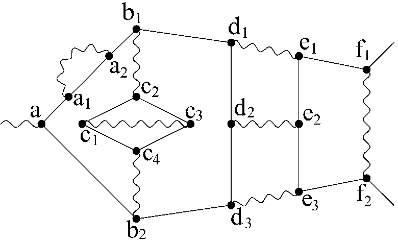
Let us examine the diagram from Fig. contributing to $a_{\mu}$, where all lepton loops correspond to electrons. The old method gives the expression

$$\left[A_{G}\left(1-U_{G_{e}}\right)\left(1-U_{G_{c}}\right)-\left(L_{G}-U_{G}\right)A_{G_{e}}\left(1-U_{G_{c}}\right)-\left(L_{G}-U_{G}\right)\left(1-L_{G_{e}}\right)A_{G_{c}}\right]$$

$$\times\left(1-U_{G_{d}}\right)\left(1-U_{c_{1}c_{2}c_{3}c_{4}}\right)\left(1-U_{c_{1}c_{2}c_{3}}-U_{c_{1}c_{3}c_{4}}\right)\left(1-U_{a_{1}a_{2}}\right),$$

where $G_{c}=aa_{1}a_{2}b_{1}b_{2}c_{1}c_{2}c_{3}c_{4}$, $G_{e}=aa_{1}a_{2}b_{1}b_{2}c_{1}c_{2}c_{3}c_{4}d_{1}d_{2}d_{3}e_{1}e_{2}e_{3}$, $G_{d}=aa_{1}a_{2}b_{1}b_{2}c_{1}c_{2}c_{3}c_{4}d_{1}d_{2}d_{3}$, the operator subscript means the subdiagram to which the operator is applied (encoded by the set of vertexes). Here all brackets should be expanded, each multiplication should be considered as a sequential transformation of the Feynman amplitudes from smaller to larger subdiagrams, all terms should be written in the same Feynman parametric space. In this example, the expression, that gives a contribution to $a_{\mu}$, contains $A$ applied to an electron subdiagram $G_{c}$. This looks like a nonsense, but the proof of the equivalence to the on-shell renormalization in  [12] does not allow to avoid these nonsense terms.

Also, an ability to preserve minimal gauge-invariant classes is important for divergence subtraction methods. Such a class is obtained from one diagram by moving internal photons along lepton loops and paths without jumping over the external photon (and without violating one-particle irreducibility). The old method preserves the classes without lepton loops  [9]. However, the proof in  [12] requires swapping the layers between subdiagrams to which $A$ is applied (like $G$, $G_{c}$, $G_{e}$); this can lead to exit from the class.

It surprisingly turned out that the drawbacks described above are fictitious: the nonsense terms are cancelled, and all gauge-invariant classes are preserved due to Ward identities of some kind. However, the old method remains redundand and nonflexible.

We use two types of Ward identities for individual lepton self-energy and vertex-like diagrams³³ 3 See examples of applying Ward identities for individual diagrams in  [13].. The first type is $\Gamma_{\mu}(p,0)=-\partial\Sigma(p)/\partial p^{\mu}$, where $\Gamma_{\mu}(p,q)$ is a vertex-like Feynman amplitude, $\Sigma(p)$ is a lepton self-energy amplitude; the $\Gamma_{\mu}$-diagrams are obtained from the $\Sigma$-diagram by inserting the external photon into all possible places on the main lepton path⁴⁴ 4 The main path is a lepton path between external lepton lines.. The second type is $\Gamma_{\mu}(p,0)=0$; here the $\Gamma_{\mu}$-diagrams are obtained from some diagram by inserting the external photon into one lepton cycle.

Let us describe the new method. We will use four operators $U_{0},U_{1},U_{2},U_{3}$ instead of $U$. $U_{0}$ is applied to photon self-energy and photon-photon scattering subdiagrams and works as in the standard renormalization. $U_{i},i=1,2,3$ are not fixed, but given by requirements (tentative):

• •

  $U_{i}$ extracts the overall UV-divergent part completely;

• •

  $U_{i}$ preserves the Ward identity: if $\Gamma_{\mu}$ and $\Sigma$ (or $\Gamma_{\mu}$ itself) satisfy the Ward identity described above, then $U_{i}\Gamma_{\mu}$ and $U_{i}\Sigma$ (or $U_{i}\Gamma_{\mu}$ itself) satisfy it too;

• •

  $U_{i}$ cancels IR divergences of the subdiagram;

• •

  $U_{i}$ extracts the mass part completely:

  $$U_{i}[a(p^{2})+b(p^{2})\not{p}]=a(m^{2})+b(m^{2})m+(\not{p}-m)(\ldots).$$

The definitions may differ for different particles. It is possible to put $U_{3}=L$.

By $\mathfrak{I}^{\prime}[G]$ we denote the set of all vertex-like subgraphs of $G$ (including $G$) lying on the main path of $G$ and having the external photon of $G$. By $\mathfrak{F}[G]$ we denote the set of all forests of UV-divergent subdiagrams of $G$ containing $G$. The expression is

$$\sum_{\begin{subarray}{c}F=\{G_{1},\ldots,G_{n}\}\in\mathfrak{F}[G]\\ G^{\prime}\in\mathfrak{I}^{\prime}[G]\cap F\end{subarray}}(-1)^{n-1}M^{G^{\prime}}_{G_{1}}M^{G^{\prime}}_{G_{2}}\ldots M^{G^{\prime}}_{G_{n}}.$$

Here $M^{G^{\prime}}_{G^{\prime\prime}}$ equals $A_{G^{\prime\prime}}$, if $G^{\prime\prime}=G^{\prime}$, $L_{G^{\prime\prime}}-(U_{1})_{G^{\prime\prime}}$, if $G^{\prime\prime}=G\neq G^{\prime}$, $L_{G^{\prime\prime}}$, if $G^{\prime}\subset G^{\prime\prime}\subset G$, $(U_{0})_{G^{\prime\prime}}$, if $G^{\prime\prime}$ is a photon self-energy or a light-by-light subgraph. In the remaining cases it equals $(U_{2})_{G^{\prime\prime}}$, if $G^{\prime\prime}$ lies on a lepton loop, $(U_{w})_{G^{\prime\prime}}$, if $G^{\prime\prime}\in\mathfrak{I}^{\prime}[G]$ and $G^{\prime\prime}\subset G^{\prime}$, $(U_{1})_{G^{\prime\prime}}$ in the other cases; here $w=3$, if $G$ has its external photon on a lepton loop, $w=1$ otherwise.

For the example from Fig.  we have $\mathfrak{I}^{\prime}[G]=\{G,G_{e}\}$ and the expression

$$\left[A_{G}\left(1-(U_{3})_{G_{e}}\right)-\left(L_{G}-(U_{1})_{G}\right)A_{G_{e}}\right]\times\left(1-(U_{2})_{G_{c}}\right)$$

$$\times\left(1-(U_{0})_{G_{d}}\right)\left(1-(U_{0})_{c_{1}c_{2}c_{3}c_{4}}\right)\left(1-(U_{2})_{c_{1}c_{2}c_{3}}-(U_{2})_{c_{1}c_{3}c_{4}}\right)\left(1-(U_{2})_{a_{1}a_{2}}\right).$$

Results of numerical tests of the methods are presented in Tables 1, 2, and 3. We use two setups: New 1 means $U_{1}=U_{2}=U$, $U_{3}=L$, New 2 means $U_{1}=U_{2}=U_{3}=U$. We use fixed masses of particles without taking into account their uncertainty: $m_{\mu}=105.658\,374\,5\,\text{MeV}$, $m_{e}=0.510\,998\,95\,\text{MeV}$, $m_{\tau}=1\,776.82\,\text{MeV}$. All results from Table 1 are in very good agreement with known values from literature. The difference between the methods used starts from four loops. The sum values in Table 2 are in good agreement with each other, with the value $0.006\,106(31)$ from  [11], and with  [30]. Diagrams 2 and 10 are the only diagrams with difference between the methods. The sum values in Table 3 are in good agreement with the value $2.907\,2(44)$ from  [11]. A difference between the methods is only in diagrams 7 and 8.

The author thanks Lidia Kalinovskaya, Gudrun Heinrich, Savely Karshenboim, Andrey Arbuzov for the important assistance, and Andrey Kataev for valuable consultations. Also, the author thanks the Laboratory of Information Technologies of JINR (Dubna, Russia) for providing an access to its computational resources and additionally the organizers of the conference FFK-2021 for providing a possibility to make a presentation. And beyond that, the author considers it proper to honor the memory of Fyodor Tkachov.

References

- [1] Hanneke D., Fogwell Hoogerheide S., Gabrielse G. Cavity Control of a Single-Electron Quantum Cyclotron: Measuring the Electron Magnetic Moment // Phys. Rev. A. — 2011. — V. 83, no. 052122. — arXiv:1009.4831 [physics.atom-ph].
- [2] Abi B. et al. [Muon g-2 Collaboration] Measurement of the Positive Muon Anomalous Magnetic Moment to 0.46 ppm // Phys. Rev. Lett. — 2021. — V. 126, no. 141801. — arXiv:2104.03281.
- [3] Bennett G.W. et al. [Muon g-2 Collaboration] Final report of the E821 muon anomalous magnetic moment measurement at BNL // Phys. Rev. D. — 2006. — V. 73, no. 072003. — arXiv:hep-ex/0602035.
- [4] Aoyama T., Kinoshita T., Nio M. Theory of the Anomalous Magnetic Moment of the Electron // Atoms. — 2019. — V. 7, no. 1. — P. 28.
- [5] Bouchendira R., Clade P., Guellati-Khélifa S., Nez F., Biraben F. New determination of the fine structure constant and test of the quantum electrodynamics // Phys. Rev. Lett. — 2011. — V. 106, no. 080801. — arXiv:1012.3627 [physics.atom-ph].
- [6] Mohr P.J., Newell D.B., Taylor B.N. CODATA Recommended Values of the Fundamental Physical Constants: 2014 // Rev. Mod. Phys. — 2016. — V. 88, no. 3,035009. — arXiv:1507.07956.
- [7] Parker R.H., Yu C., Zhong W., Estey B., Müller H. Measurement of the fine-structure constant as a test of the Standard Model // Science. — 2018. — V. 360. — P. 191. — arXiv:1812.04130.
- [8] Morel L., Yao Z., Cladé P., Guellati-Khélifa S. Determination of the fine-structure constant with an accuracy of 81 parts per trillion // Nature. — 2020. — V. 588, no. 7836. — P. 61–65.
- [9] Volkov S. Calculating the five-loop QED contribution to the electron anomalous magnetic moment: Graphs without lepton loops // Phys. Rev. D. — 2019. — V. 100, no. 9,096004. — arXiv:1909.08015.
- [10] Aoyama T., Asmussen N., others. The anomalous magnetic moment of the muon in the Standard Model // Physics Reports. — 2020. — V. 887. — P. 1–166. — arXiv:2006.04822.
- [11] Aoyama T., Hayakawa M., Kinoshita T., Nio M. Complete Tenth-Order QED Contribution to the Muon g-2 // Phys. Rev. Lett. — 2012. — V. 109, no. 111808. — arXiv:1205.5370 [hep-ph].
- [12] Volkov S. Subtractive procedure for calculating the anomalous electron magnetic moment in QED and its application for numerical calculation at the three-loop level // J. Exp. Theor. Phys. — 2016. — V. 122, no. 6. — P. 1008–1031.
- [13] Volkov S. Numerical calculation of high-order QED contributions to the electron anomalous magnetic moment // Phys. Rev. D. — 2018. — V. 98, no. 7,076018. — arXiv:1807.05281.
- [14] Laporta S., Remiddi E. The Analytical value of the electron (g-2) at order in QED // Phys. Lett. B. — 1996. — V. 379. — P. 283. — arXiv:hep-ph/9602417.
- [15] Laporta S. The Analytical value of the corner ladder graphs contribution to the electron (g-2) in QED // Phys. Lett. B. — 1995. — V. 343. — P. 421–426.
- [16] Barbieri R., Caffo M., Remiddi E., Turrini S., Oury D. The anomalous magnetic moment of the electron in QED: some more sixth order contributions in the dispersive approach // Nuclear Physics B. — 1978. — V. 144. — P. 329–348.
- [17] Levine M.J., Roskies R. Analytic contribution to the factor of the electron in sixth order // Phys. Rev. D. — 1976. — V. 14. — P. 2191.
- [18] Levine M.J., Perisho R.C., Roskies R. Analytic Contributions to the G Factor of the electron // Phys. Rev. D. — 1976. — V. 13. — P. 997.
- [19] Levine M.J., Remiddi E., Roskies R. Analytic Contributions To The G Factor Of The Electron In Sixth Order // Phys. Rev. D. — 1979. — V. 20. — P. 2068–2076.
- [20] Levine M.J., Roskies R. Hyperspherical approach to quantum electrodynamics - sixth-order magnetic moment // Phys. Rev. D. — 1974. — V. 9. — P. 421.
- [21] Barbieri R., Remiddi E. Sixth order electron and muon from second order vacuum polarization insertion // Physics Letters B. — 1974. — V. 49. — P. 468.
- [22] Barbieri R., Caffo M., Remiddi E. A Contribution to Sixth Order electron and Muon Anomalies. 3. // Lett. Nuovo Cimento. — 1974. — V. 9. — P. 690.
- [23] Billi D., Caffo M., Remiddi E. A Contribution to the sixth-Order electron and muon Anomalies // Lettere al Nuovo Cimento. — 1972. — V. 4, no. 14. — P. 657–660.
- [24] Barbieri R., Caffo M., Remiddi E. A contribution to sixth-order electron and muon anomalies. – II // Lett. Nuovo Cimento. — 1972. — V. 5. — P. 769.
- [25] Mignaco J., Remiddi E. Fourth-order vacuum polarization contribution to the sixth-order electron magnetic moment // Nuovo Cimento A. — 1969. — V. 60. — P. 519.
- [26] Laporta S., Remiddi E. The Analytic value of the light-light vertex graph contributions to the electron (g-2) in QED // Phys. Lett. B. — 1991. — V. 265. — P. 182–184.
- [27] Laporta S. The Analytical contribution of the sixth order graphs with vacuum polarization insertions to the muon (g-2) in QED // Nuovo Cimento A. — 1993. — V. 106, no. 5. — P. 675–683.
- [28] Laporta S., Remiddi E. The Analytical value of the electron light-light graphs contribution to the muon (g-2) in QED // Physics Letters B. — 1993. — V. 301. — P. 440–446.
- [29] Czarnecki A., Skrzypek M. The Muon anomalous magnetic moment in QED: Three loop electron and tau contributions // Physics Letters B. — 1999. — V. 449. — P. 354–360. — arXiv:hep-ph/9812394.
- [30] Kurz A., Liu T., Marquard P., Steinhauser M. Anomalous magnetic moment with heavy virtual leptons // Nucl. Phys. B. — 2014. — V. 879. — P. 1–18. — arXiv:1311.2471 [hep-ph].