New Physics Hints from Flavour

The Standard Model (SM) can be succinctly described as the most general renormalizable theory of quarks, leptons and the Higgs field, invariant under the electroweak gauge group:

Renormalizability implies scale-independent self-consistency, in the sense that, from a purely theoretical point of view, the validity of the SM can be extended up to arbitrarily high energy scales¹¹ 1 This is admittedly an oversimplification, for our discussion ignores both the problems of vacuum stability [48] and of potential Landau poles [49, 50] in the renormalization group flow of SM couplings. While, from a purely theoretical point of view, both these issues should be considered seriously, the involved energy scales are usually several order of magnitudes higher than effective cut-offs coming from the explicit introduction of a non-renormalizable interaction in the theory.. On the other hand, as discussed in the Introduction, there are irrefutable reasons to believe that the SM is not the ultimate theory of Nature, which in turn makes renormalizability a dispensable, if not unmotivated, feature for a realistic theory. Dropping the renormalizability requirement leads from the ultraviolet complete SM theory to an Effective Field Theory (EFT) known as Standard Model Effective Field Theory (SMEFT) [51, 52].

Any quantum field theory with the same light degrees of freedom as the SM, plus some extra heavy degree of freedom, is correctly described by SMEFT at sufficiently low energies (that is, below the EFT cut-off, which is usually of order of the lightest new particle mass). Altough this case does not cover all conceivable generalizations of the SM²² 2 For instance, theories which extend the SM with light, feebly coupled degrees of freedom, such as axions or light singlet neutrinos, cannot be directly described by SMEFT., it definitely includes a large majority of phenomenological theories which attempt to address one or more SM shortcomings.

In what follows we review the standard SMEFT construction [51, 52] and set our SMEFT notations. The quantum numbers of SM fields under $G_{\text{SM}}$ are collected in Table 1.1, together with their Lorentz representations. From Table 1.1, we can immediately construct the SM lagrangian density (or, simply, “lagrangian”):

In the equations above, $\widetilde{H}$ denotes the conjugate Higgs field $\widetilde{H}=i\sigma_{2}H^{*}$, and $D_{\mu}$ is the gauge covariant derivative, defined by:

where the generators $T^{(3,2)}$ and $Y$ are given in the relevant representations; we will also occasionally employ the notation $\phi_{1}\overleftrightarrow{D_{\mu}}\phi_{2}=\phi_{1}D_{\mu}\phi_{2}-(D_{\mu}\phi_{1})\phi_{2}$. All constants appearing in Eqs. (1.1.3)-(1.1.5) have been experimentally measured [9] (except for the QCD $\theta$ angle, for which only an upper bound exists [53]).

A key ingredient in postulating the SM lagrangian (1.1.2) is renormalizability, which is simply implemented by the requirement that all SM operators have mass dimension at most four (the space-time dimension). Together with gauge invariance, it fully determines the (finite) list of operators which can appear on the right-hand side of Eq. (1.1.2). On the other hand, if renormalizability is not required, it does still make sense to consider Eq. (1.1.2) as the leading order expansion of a non-renormalizable lagrangian, the SMEFT lagrangian, whose higher dimensional operator coefficients are unknown. Concretely, we take:

In the previous equation, the sum extends over all gauge-invariant operators $\mathcal{O}$ with mass dimension $d_{\mathcal{O}}>4$ which can be built out of the SM fields; $\Lambda_{\mathcal{O}}$ is an energy scale specific to the operator $\mathcal{O}$ and $c_{\mathcal{O}}$ is a dimensionless coefficient of $\mathcal{O}((4\pi)^{-\ell})$, where $\ell$ is the loop-order at which the operator is generated; the combination $C_{\mathcal{O}}=c_{\mathcal{O}}\Lambda_{\mathcal{O}}{}^{4-d_{\mathcal{O}}}$ defines the so-called Wilson coefficient of the operator $\mathcal{O}$. The effects of $\mathcal{O}$ at experimental energies $E$ are suppressed by a factor of $C_{\mathcal{O}}E^{d_{\mathcal{O}}-4}=c_{\mathcal{O}}(E/\Lambda_{\mathcal{O}})^{d_{\mathcal{O}}-4}$, which could explain why conclusive evidence of deviations from the SM is still lacking. The non-renormalizable theory defined by (1.1.7) has an implicit energy cut-off $\Lambda_{\text{SMEFT}}$, which restricts its validity to energies $E\leq\Lambda_{\text{SMEFT}}$, and is expected to be of the same order of the smallest operator scales $\Lambda_{\mathcal{O}}$.

In practice, only operators with mass dimension up to a maximal value are included in Eq. (1.1.7). Truncating the sum at dimension five, the only extra non-renormalizable operator is the well known Weinberg operator [54]:

together with its hermitian conjugate (here $\mathscr{C}$ denotes the Dirac charge conjugation matrix). At dimension six, the list of effective operators is much richer and consists of 59 independent operators, which we report in Tables 1.2 to 1.5 in the so-called Warsaw basis [52].

The precise sense in which Warsaw basis operators are independent is the following: none of the operators in Tables 1.2-1.5 can be obtained from the remaining ones by taking linear combinations, adding a total divergence, or applying smooth field redefinitions (as its name suggests, the Warsaw basis is also complete, in the sense that any dimension six operator can be obtained from Warsaw basis operators by means of these three operations). The last requirement follows from a well known theorem [55, 56] which states that for any smooth transformation $\phi\mapsto F(\phi)$ of the coordinate fields $\phi$, the two quantum lagrangians $\mathcal{L}$ and $\mathcal{L}^{\prime}=\mathcal{L}\circ F$ give rise to the same physical $S$ matrix.

To conclude this Section, we observe that the SMEFT formalism we have just described allows one to obtain low energy parametrizations of, virtually, any SM extension by heavy new fields. The procedure by which one can pass from a high-energy ultraviolet complete model to the low-energy SMEFT description is called matching, and is the object of the next Section.

The standard matching of EFTs enforces the physical equivalence between an high-energy theory and an effective theory with a reduced number of light degrees of freedom, by requiring equality between the Green’s functions³³ 3 This is actually stronger than requiring the equality of (physical) $S$-matrix elements, but does not imply a loss in generality. In fact, given a theory with lagrangian $\mathcal{L}(\phi,\Phi)$, where $\phi$ and $\Phi$ denote the set of light and heavy fields respectively, we can always define a low-energy theory by the lagrangian: $$\mathcal{L}_{\text{EFT}}(\phi)=\log\left\{\intop\mathcal{D}\Phi\,\exp\left[\mathcal{L}(\phi,\Phi)\right]\right\}.$$ By construction, $\mathcal{L}_{\text{EFT}}$ and $\mathcal{L}$ give rise to the same $\phi$ Green’s functions, and the scale separation between $\phi$ and $\Phi$ fields ensures that $\mathcal{L}_{\text{EFT}}$ can be expanded in a series of local operators. of light fields computed in the two theories at a fixed renormalization scale $\mu$. The latter is typically chosen to be close to the typical mass scale $M$ of the fields being integrated out⁴⁴ 4 We assume here that there exists only one such scale. In the presence of several scales $M_{1}\ll M_{2}\ll\cdots\ll M_{n}$ with sizable separations, the matching is usually performed in a sequential fashion, connecting the various scales $M_{i}$ and $M_{i+1}$ using the renormalization group flow of the intermediate EFTs resulting from the procedure., to ensure that the matching conditions can be computed perturbatively, as $l$-loop diagrams can contribute to the matching equations with terms proportional to $(4\pi)^{-l}\ln(\mu/M)^{l-i}$ for $i=0,\,1,\,\dots,\,l$ [57].

In practice, it is sufficient to enforce matching for the so-called 1-Light-Particle Irreducible (1LPI) Green’s functions of the light fields, which are defined as sums of connected Feynman graphs which do not have a single line cut corresponding to an internal light field exchange. At a fixed maximal power $M^{-k}$ in the EFT expansion, only a finite number of 1LPI Green’s function receive contributions from integrating out the heavy fields in the high-energy theory, and each of these gives rise to an independent matching equation for the Wilson coefficients of EFT operators of dimension $d\leq 4+k$. Concretely, a sample computation would go as follows [57, 58]:

1. (1)

   Compute the 1LPI Green’s function in the high-energy theory, expanding in powers of $\frac{1}{M}$ up to the desired order.

2. (2)

   Compute the same function in the EFT, including the contributions from effective operators with unknown (as yet) Wilson coefficients.

3. (3)

   Equate the two results.

It goes without mention that steps 1 and 2 above can usually be carried out only in a perturbative fashion, i.e. expanding the corresponding Green’s function to a fixed loop order (which should be the same in the high-energy and effective theories). The output of this procedure is the full list of EFT Wilson coefficients at the given loop accuracy, which are usually reported in a standard basis, such as the Warsaw basis for SMEFT dimension-six operators.

Adopting a standard operator basis is useful for communicating the final results of an EFT calculation in a compact and unambiguous manner. That said, the diagrammatic matching calculations described above are most naturally performed using a larger effective operator basis, which I will refer to as the Green’s basis, following the terminology of Ref. [59]. In defining Green’s basis operators, we drop the requirement of independence under field redefinitions; the Green’s basis is the correct operator menu to be used in the second step of the matching procedure described above, since there exists a bijective linear correspondence between dimension-$d$ Green’s operators and Green’s functions.

Simplifying EFT calculations can provide great help to BSM phenomenologists, by accelerating the process of model building and evaluation. There are two main possible sources of simplification, namely: mathematical methods and automation.

On the mathematical side, the problem of SMEFT tree-level matching up to dimension-six terms was completely solved in Ref. [60], which provided the complete dictionary of SMEFT contributions for all possible tree-level mediators. The key observation behind this work is that, for any fixed maximal effective operator dimension, the number of extra fields and couplings which can give rise to SMEFT operators at low energies is finite, so that the program of Ref. [60] can, at least in principle, be carried out up to any effective operator dimension.

Unfortunately, such a simplification no longer occurs for $\ell\geq 1$-loop contributions, in which case more general methods are required. In particular, functional methods (focusing on Green’s function generating functionals) have provided significant advances in the context of one-loop computations, the latest approaches being based on the so-called Universal One-Loop Effective Action (UOLEA) [61], which generalises methods based on the Covariant Derivative Expansion (CDE) [62], but whose formalism is still incomplete (see Ref. [61] and references therein for a recent discussion, and for an application of the UOLEA formalism).

Concerning automated methods, many general tools aimed at simplifying EFT calculations are already available (for a comprehensive review, see [63] and references therein). For the specific task of EFT matching, however, the tool-set is still for a large part under development. We cite here the software packages mentioned in Ref. [63]:

• •

  MatchingTools [64], a Python library providing support for tree-level matching of generic field theories (i.e. not restricted by the SM gauge group and field content). This package was used, in particular, for an extensive check of the analytic results provided by Ref. [60] mentioned earlier.

• •

  CoDEx [65], a Mathematica package devoted to SMEFT matching at one-loop and up to dimension-six operators. CoDEx is based on the Covariant Derivative Expansions, and the latest release (v1.0.0) by the time of this writing can correctly handle only one-loop diagrams not involving light internal particles in the loop.

• •

  MatchMaker [63], a work-in-progress Python package whose primary purpose is, again, the complete SMEFT one-loop matching (with the grand goal of extending the tool-set to arbitrary field theories). Unfortunately, by the time of this writing, no further update on the progress status of MatchMaker is available.

To conclude, both mathematical and computer-based methods for EFT calculations still offer large room for improvement, and progress in this area could definitely provide precious help in our meandering search for BSM signals.

The UV model under consideration is defined by the SM gauge group and field content, with the addition of two colored scalar leptoquarks:

where in parenthesis we indicate the $S_{1,3}$ representations under $\left(\text{SU}(3)_{c},\,\text{SU}(2)_{L}\right)_{\text{U}(1)_{Y}}$. At the renormalizable level, the two additional scalars directly couple to SM fermions through the Yukawa terms:

(hence the name “leptoquarks”). The couplings in Eq. (2.1.2) by themselves do not imply a violation of baryon or lepton number conservation, as can be seen by the $S_{1/3}$ lepton and baryon number assignments:

On the other hand, the following additional “diquark” operators are also allowed by gauge invariance:

which violate baryon number conservation according to Eq. (2.1.3), and may lead, e.g., to proton decay. As a consequence, since the phenomenological motivations mentioned above require the introduction of relatively low-scale NP degrees of freedom (of order $\mathcal{O}(\text{TeV})$, say), baryon and lepton number conservation is actually postulated a priori¹¹ 1 See Ref. [70] for an extended gauge model involving $S_{1}$ and $S_{3}$, in which lepton and baryon number are accidental symmetries, as in the SM., along with Eq. (2.1.3), which allows the leptoquark couplings (2.1.2) but forbids the diquark ones, Eq. (2.1.4). Finally, the addition of $S_{1/3}$ also gives rise to a scalar potential:

where $\Delta\mathcal{V}_{S}$ denotes trilinear and tetralinear terms in the $S_{1/3}$ and Higgs fields, which we omit here for brevity (the full expression is reported in Sec. 2.5).

The leptoquark couplings in Eq. (2.1.2), as well as the omitted potential couplings in Eq. (2.1.5)) are assumed to be in the perturbative regime²² 2 See Ref. [71] for an analysis of perturbativity bounds from unitarity principles., so that theory quantities such as Green’s functions admit a sensible perturbative expansion, which, following standard arguments [72], is equivalent to a loop-wise expansion in Feynman graph calculations. Assuming the leptoquark masses $M_{1}^{2}$ and $M_{3}^{2}$ to be of similar order of magnitude (and, of course, large with respect to the electroweak scale), it is easy³³ 3 These can be easily obtained by replacing $S_{1}$ and $S_{3}$ in the leptoquark model’s lagrangian with the corresponding solutions (in terms of SM fields) of the classical Equations Of Motion (EOM). In doing this, one should take into account the following simplifications, which reduce the problem at hand to linear algebra: (1) Terms in the scalar potential (2.1.5) which are not quadratic in $S_{1/3}$ do not contribute to tree-level matching at leading dimension, and can be safely omitted from the EOM. (2) Covariant derivative terms (i.e. $\left|D_{\mu}S_{1,3}\right|^{2}$) from the kinetic lagrangian also give rise to higher ($\geq 8$) dimensional operators, and can be disregarded for the purpose of tree-level matching. to obtain the tree-level, dimension-six SMEFT matching conditions for the (lepton-baryon number conserving) $S_{1}+S_{3}$ model:

The Wilson coefficient notation refers to the Warsaw basis (Tables 1.2-1.5). The suffixes ⁽⁰⁾ indicate the accuracy (in terms of loop orders, here zero) of Eqs. (2.1.6)-(2.1.10), and the RG sliding scale $\mu$ is assumed to be close in magnitude to $M_{1,3}^{2}$ (the running UV couplings in the right-hand sides of Eqs. (2.1.6)-(2.1.10) are understood to be evaluated at the same scale).

In general, taking perturbativity as given, Wilson coefficients admit a loop-wise expansion of the form:

Going beyond the tree-level matching, apart from the (obviously) increased computational complexity, a few other technicalities need to be taken into account:

1. (1)

   Loop computations require the introduction of a renormalization scheme, which must be entirely specified along with the final (renormalized) results. We employ the $\overline{\text{MS}}$ scheme with the Naive Dimensional Regularization (NDR) prescription for analytically extending Dirac matrices to arbitrary real dimensions $d=4-2\epsilon$. Furthermore, all computations are performed in a generic $R_{\xi}$ gauge, in order to check for the expected elision of $\xi$-dependencies in the Wilson coefficients of gauge invariant operators.

2. (2)

   A further scheme-dependence can (and does, in our case) arise from the prescriptions adopted for evanescent operators [73], which are Dirac operators that vanish in four dimension, but may be non-vanishing in $d=4-2\epsilon$⁴⁴ 4 An instructive example is given by the two Dirac tensors: $\displaystyle\mathcal{E}_{1}$ $\displaystyle=P_{L}\gamma^{\mu}\gamma^{\nu}P_{L}\otimes P_{L}\gamma_{\mu}\gamma_{\nu}P_{L}-4P_{L}\otimes P_{L}+P_{L}\sigma^{\mu\nu}P_{L}\otimes P_{L}\sigma_{\mu\nu}P_{L},$ $\displaystyle\mathcal{E}_{2}$ $\displaystyle=P_{L}\gamma^{\mu}\gamma^{\nu}P_{L}\otimes P_{R}\gamma_{\mu}\gamma_{\nu}P_{R}-4P_{L}\otimes P_{R}.$ Following the NDR prescription for the Dirac algebra in dimension $d=4-2\epsilon$: $$\left\{\gamma^{\mu},\gamma^{\nu}\right\}=2\eta^{\mu\nu},\qquad\left\{\gamma^{\mu},\gamma^{5}\right\}=0,\qquad\text{Tr}(\eta)=4-2\epsilon,$$ one can easily work out the result $\mathcal{E}_{1}=-2\epsilon P_{L}\otimes P_{L}$. However, the operator $\mathcal{E}_{2}$ is not univocally fixed by the NDR rules, and $\mathcal{E}_{2}$ is usually expressed in terms of canonical Dirac tensors as follows [74]: $$\mathcal{E}_{2}=4a_{\text{ev}}\epsilon P_{L}\otimes P_{R}+E_{LR}^{(2)}(a_{\text{ev}}),$$ where the actual form of $E_{LR}^{(2)}(a_{\text{ev}})$ in the right-hand side depends on the value of $a_{\text{ev}}$, which is completely arbitrary and should be regarded as part of the regularization scheme (for $a_{\text{ev}}=-\frac{1}{2}$ one gets $E_{LR}^{(2)}(a_{\text{ev}})=P_{L}\sigma^{\mu\nu}P_{L}\otimes P_{R}\sigma_{\mu\nu}P_{R}$, cf. Ref. [74]).. We follow the conventions of Ref. [74], keeping the scheme-defining coefficients $\left\{a_{\text{ev}},\,b_{\text{ev}},\,...\right\}$ arbitrary in our computations (in practice, the only coefficient entering one-loop computations is $a_{\text{ev}}$).

3. (3)

   As discussed in Sec. 1.2, diagrammatic matching computations are naturally performed in the Green’s basis. An important result of Ref. [44] was thus (i) to classify all SMEFT dimension-six Green’s basis operators, and (ii) to provide a set of (linear) reduction equations which allow to pass from the Green’s basis to the standard Warsaw basis, after field redefinition redundancy is properly taken into account.

4. (4)

   Integrating out the leptoquarks at one loop also generates contributions to SM renormalizable operators and, in particular, fermion kinetic terms. Such modifications can be undone by suitable field and SM coupling redefinitions, which however also introduce additional contributions to tree-level generated WCs⁵⁵ 5 Since field redefinitions arise at one loop in our model, only tree-level WCs are affected. In general, any tree-level shift in SM couplings and wave-function renormalizations that could influence loop-generated coefficients should be taken into account, see e.g. [59].. In our case only fermion kinetic terms (i.e. wave-functions renormalizations) are relevant, as the tree-level WCs in Eqs. (2.1.6)-(2.1.10) do not depend on any SM coupling. The one-loop formulas below include the contributions due to fermion field renormalization.

In what follows we illustrate the diagrammatic matching steps with a fully detailed example, and subsequently review the procedures used in Ref. [44] to obtain a dimension-six SMEFT Green’s basis and the corresponding equations for reduction onto the Warsaw basis. For additional details, including the final complete results for the SMEFT Wilson coefficients of the $S_{1}+S_{3}$ model, we address the reader to the original reference [44].

In this Section we discuss in some details the matching of a specific Green’s function, in order to illustrate some of the most relevant aspects of our computation.

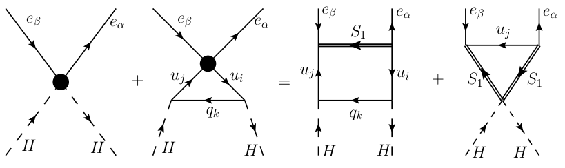
Let us consider the off-shell Green’s function $\mathcal{G}\equiv\langle e_{\beta}(p_{1})\bar{e}_{\alpha}(p_{2})H_{b}(q_{1})H_{a}^{\dagger}(q_{2})\rangle$, where all momenta are incoming and $a,\,b$ are $\text{SU}(2)_{L}$ indices. The matching conditions for this correlator are depicted diagrammatically in Fig. 2.3.1, where the left and right hand-side show the EFT and UV contributions, respectively. We briefly comment on the various steps of this computation.

We begin by listing the various contributions to $\mathcal{G}$, both in the SMEFT and the leptoquark model. The SMEFT operators which contribute at tree level to $\mathcal{G}$ are (cf. Table 2.2 for the notation):

Moreover, we must take into account a one-loop contribution from $\mathcal{O}_{eu}$, which is generated at the tree-level in our model according to Eq. (2.1.10). Since this tree-level WC is fixed, the matching of $\mathcal{G}$ allows us to fix the coefficients of the operators in Eqs. (2.3.1)-(2.3.3), see the left-hand side of Fig. 2.3.1. In the leptoquark model there are two diagrams contributing to $\mathcal{G}$, both mediated by $S_{1}$, shown on the right-hand side of Fig. 2.3.1: a box diagram proportional to (schematically) $y_{U}y_{U}^{\dagger}\lambda^{1R}\lambda^{1R}{}^{\dagger}$, and a triangle diagram proportional to $\lambda_{H1}\lambda^{1R}{}^{\dagger}\lambda^{1R}$ (the coupling $\lambda_{H1}$ is defined in Eq. (2.5.1)).

By total momentum conservation, only three out of the four momenta $p_{1},\,p_{2},\,q_{1},\,q_{2}$ are independent. Writing $(p_{1},p_{2},q_{1},q_{2})=(p-r,\,-p-r,\,q+r,\,-q+r)$, the tree-level contributions from the operators in Eqs. (2.3.1)-(2.3.3) read:

where we drop here and below a global $\delta_{ab}$ factor, and we denote Green’s basis WCs by $G_{i}$. The UV and EFT one-loop contributions are more easily computed when only one of the independent momenta $p,\,q,\,r$ is non-vanishing, and yield respectively:

References

- [1] S. L. Glashow, Partial Symmetries of Weak Interactions, Nucl. Phys. 22 (1961) 579–588.
- [2] S. Weinberg, A Model of Leptons, Phys. Rev. Lett. 19 (1967) 1264–1266.
- [3] A. Salam, Weak and Electromagnetic Interactions, Conf. Proc. C 680519 (1968) 367–377.
- [4] ATLAS Collaboration, G. Aad et al., Observation of a new particle in the search for the Standard Model Higgs boson with the ATLAS detector at the LHC, Phys. Lett. B 716 (2012) 1–29, [arXiv:1207.7214].
- [5] CMS Collaboration, S. Chatrchyan et al., Observation of a New Boson at a Mass of 125 GeV with the CMS Experiment at the LHC, Phys. Lett. B 716 (2012) 30–61, [arXiv:1207.7235].
- [6] P. W. Higgs, Broken Symmetries and the Masses of Gauge Bosons, Phys. Rev. Lett. 13 (1964) 508–509.
- [7] F. Englert and R. Brout, Broken Symmetry and the Mass of Gauge Vector Mesons, Phys. Rev. Lett. 13 (1964) 321–323.
- [8] G. S. Guralnik, C. R. Hagen, and T. W. B. Kibble, Global Conservation Laws and Massless Particles, Phys. Rev. Lett. 13 (1964) 585–587.
- [9] Particle Data Group Collaboration, P. Zyla et al., Review of Particle Physics, PTEP 2020 (2020), no. 8 083C01.
- [10] A. Romanino, Naturalness After LHC run I, Frascati Phys. Ser. 61 (2016) 26–34.
- [11] C. Gross, A. Polosa, A. Strumia, A. Urbano, and W. Xue, Dark Matter in the Standard Model?, Phys. Rev. D 98 (2018), no. 6 063005, [arXiv:1803.10242].
- [12] G. ’t Hooft, Naturalness, chiral symmetry, and spontaneous chiral symmetry breaking, NATO Sci. Ser. B 59 (1980) 135–157.
- [13] G. F. Giudice, Naturally Speaking: The Naturalness Criterion and Physics at the LHC, arXiv:0801.2562.
- [14] F. Feruglio, Pieces of the Flavour Puzzle, Eur. Phys. J. C 75 (2015), no. 8 373, [arXiv:1503.04071].
- [15] BaBar Collaboration, J. Lees et al., Evidence for an excess of decays, Phys. Rev. Lett. 109 (2012) 101802, [arXiv:1205.5442].
- [16] BaBar Collaboration, J. Lees et al., Measurement of an Excess of Decays and Implications for Charged Higgs Bosons, Phys. Rev. D 88 (2013), no. 7 072012, [arXiv:1303.0571].
- [17] LHCb Collaboration, R. Aaij et al., Measurement of the ratio of branching fractions , Phys. Rev. Lett. 115 (2015), no. 11 111803, [arXiv:1506.08614]. [Erratum: Phys.Rev.Lett. 115, 159901 (2015)].
- [18] Belle Collaboration, M. Huschle et al., Measurement of the branching ratio of relative to decays with hadronic tagging at Belle, Phys. Rev. D 92 (2015), no. 7 072014, [arXiv:1507.03233].
- [19] Belle Collaboration, Y. Sato et al., Measurement of the branching ratio of relative to decays with a semileptonic tagging method, Phys. Rev. D 94 (2016), no. 7 072007, [arXiv:1607.07923].
- [20] Belle Collaboration, S. Hirose et al., Measurement of the lepton polarization and in the decay , Phys. Rev. Lett. 118 (2017), no. 21 211801, [arXiv:1612.00529].
- [21] Belle Collaboration, S. Hirose et al., Measurement of the lepton polarization and in the decay with one-prong hadronic decays at Belle, Phys. Rev. D 97 (2018), no. 1 012004, [arXiv:1709.00129].
- [22] LHCb Collaboration, R. Aaij et al., Measurement of the ratio of the and branching fractions using three-prong -lepton decays, Phys. Rev. Lett. 120 (2018), no. 17 171802, [arXiv:1708.08856].
- [23] LHCb Collaboration, R. Aaij et al., Test of Lepton Flavor Universality by the measurement of the branching fraction using three-prong decays, Phys. Rev. D 97 (2018), no. 7 072013, [arXiv:1711.02505].
- [24] LHCb Collaboration, B. Siddi, Measurement of R() with hadronic decays, J. Phys. Conf. Ser. 956 (2018), no. 1 012015.
- [25] Belle Collaboration, G. Caria et al., Measurement of and with a semileptonic tagging method, Phys. Rev. Lett. 124 (2020), no. 16 161803, [arXiv:1910.05864].
- [26] LHCb Collaboration, R. Aaij et al., Measurement of Form-Factor-Independent Observables in the Decay , Phys. Rev. Lett. 111 (2013) 191801, [arXiv:1308.1707].
- [27] LHCb Collaboration, R. Aaij et al., Test of lepton universality using decays, Phys. Rev. Lett. 113 (2014) 151601, [arXiv:1406.6482].
- [28] LHCb Collaboration, R. Aaij et al., Angular analysis of the decay using 3 fb-1 of integrated luminosity, JHEP 02 (2016) 104, [arXiv:1512.04442].
- [29] LHCb Collaboration, R. Aaij et al., Angular analysis and differential branching fraction of the decay , JHEP 09 (2015) 179, [arXiv:1506.08777].
- [30] LHCb Collaboration, R. Aaij et al., Measurement of the branching fraction and effective lifetime and search for decays, Phys. Rev. Lett. 118 (2017), no. 19 191801, [arXiv:1703.05747].
- [31] LHCb Collaboration, R. Aaij et al., Test of lepton universality with decays, JHEP 08 (2017) 055, [arXiv:1705.05802].
- [32] ATLAS Collaboration, M. Aaboud et al., Study of the rare decays of and mesons into muon pairs using data collected during 2015 and 2016 with the ATLAS detector, JHEP 04 (2019) 098, [arXiv:1812.03017].
- [33] LHCb Collaboration, R. Aaij et al., Search for lepton-universality violation in decays, Phys. Rev. Lett. 122 (2019), no. 19 191801, [arXiv:1903.09252].
- [34] Belle Collaboration, A. Abdesselam et al., Test of lepton flavor universality in decays at Belle, arXiv:1904.02440.
- [35] LHCb Collaboration, R. Aaij et al., Measurement of -Averaged Observables in the Decay, Phys. Rev. Lett. 125 (2020), no. 1 011802, [arXiv:2003.04831].
- [36] LHCb Collaboration, R. Aaij et al., Test of lepton universality in beauty-quark decays, arXiv:2103.11769.
- [37] D. Lancierini, G. Isidori, P. Owen, and N. Serra, On the significance of new physics in decays, arXiv:2104.05631.
- [38] S. Bifani, S. Descotes-Genon, A. Romero Vidal, and M.-H. Schune, Review of Lepton Universality tests in decays, J. Phys. G 46 (2019), no. 2 023001, [arXiv:1809.06229].
- [39] L. Di Luzio and M. Nardecchia, What is the scale of new physics behind the -flavour anomalies?, Eur. Phys. J. C 77 (2017), no. 8 536, [arXiv:1706.01868].
- [40] T. Nomura and T. Shimomura, Search for pair production from scalar boson decay in minimal model at the LHC, Eur. Phys. J. C 81 (2021), no. 4 297, [arXiv:2012.13049].
- [41] I. Esteban, M. C. Gonzalez-Garcia, M. Maltoni, T. Schwetz, and A. Zhou, The fate of hints: updated global analysis of three-flavor neutrino oscillations, JHEP 09 (2020) 178, [arXiv:2007.14792].
- [42] KATRIN Collaboration, M. Aker et al., Improved Upper Limit on the Neutrino Mass from a Direct Kinematic Method by KATRIN, Phys. Rev. Lett. 123 (2019), no. 22 221802, [arXiv:1909.06048].
- [43] F. Feruglio, Are neutrino masses modular forms? 2019. arXiv:1706.08749.
- [44] V. Gherardi, D. Marzocca, and E. Venturini, Matching scalar leptoquarks to the SMEFT at one loop, JHEP 07 (2020) 225, [arXiv:2003.12525].
- [45] V. Gherardi, D. Marzocca, M. Nardecchia, and A. Romanino, Rank-One Flavor Violation and B-meson anomalies, JHEP 10 (2019) 112, [arXiv:1903.10954].
- [46] V. Gherardi, D. Marzocca, and E. Venturini, Low-energy phenomenology of scalar leptoquarks at one-loop accuracy, JHEP 01 (2021) 138, [arXiv:2008.09548].
- [47] F. Feruglio, V. Gherardi, A. Romanino, and A. Titov, Modular invariant dynamics and fermion mass hierarchies around , JHEP 05 (2021) 242, [arXiv:2101.08718].
- [48] G. Degrassi, S. Di Vita, J. Elias-Miro, J. R. Espinosa, G. F. Giudice, G. Isidori, and A. Strumia, Higgs mass and vacuum stability in the Standard Model at NNLO, JHEP 08 (2012) 098, [arXiv:1205.6497].
- [49] M. Gell-Mann and F. E. Low, Quantum electrodynamics at small distances, Phys. Rev. 95 (1954) 1300–1312.
- [50] M. Gockeler, R. Horsley, V. Linke, P. E. L. Rakow, G. Schierholz, and H. Stuben, Is there a Landau pole problem in QED?, Phys. Rev. Lett. 80 (1998) 4119–4122, [hep-th/9712244].
- [51] W. Buchmuller and D. Wyler, Effective Lagrangian Analysis of New Interactions and Flavor Conservation, Nucl. Phys. B 268 (1986) 621–653.
- [52] B. Grzadkowski, M. Iskrzynski, M. Misiak, and J. Rosiek, Dimension-Six Terms in the Standard Model Lagrangian, JHEP 10 (2010) 085, [arXiv:1008.4884].
- [53] J. E. Kim and G. Carosi, Axions and the Strong CP Problem, Rev. Mod. Phys. 82 (2010) 557–602, [arXiv:0807.3125]. [Erratum: Rev.Mod.Phys. 91, 049902 (2019)].
- [54] S. Weinberg, Baryon and Lepton Nonconserving Processes, Phys. Rev. Lett. 43 (1979) 1566–1570.
- [55] S. Kamefuchi, L. O’Raifeartaigh, and A. Salam, Change of variables and equivalence theorems in quantum field theories, Nucl. Phys. 28 (1961) 529–549.
- [56] M. Bando, T. Kugo, and K. Yamawaki, Nonlinear Realization and Hidden Local Symmetries, Phys. Rept. 164 (1988) 217–314.
- [57] H. Georgi, Effective field theory, Ann. Rev. Nucl. Part. Sci. 43 (1993) 209–252.
- [58] A. J. Buras, Weak Hamiltonian, CP violation and rare decays, in Les Houches Summer School in Theoretical Physics, Session 68: Probing the Standard Model of Particle Interactions, pp. 281–539, 6, 1998. hep-ph/9806471.
- [59] M. Jiang, N. Craig, Y.-Y. Li, and D. Sutherland, Complete One-Loop Matching for a Singlet Scalar in the Standard Model EFT, JHEP 02 (2019) 031, [arXiv:1811.08878].
- [60] J. de Blas, J. C. Criado, M. Perez-Victoria, and J. Santiago, Effective description of general extensions of the Standard Model: the complete tree-level dictionary, JHEP 03 (2018) 109, [arXiv:1711.10391].
- [61] U. Haisch, M. Ruhdorfer, E. Salvioni, E. Venturini, and A. Weiler, Singlet night in Feynman-ville: one-loop matching of a real scalar, JHEP 04 (2020) 164, [arXiv:2003.05936]. [Erratum: JHEP 07, 066 (2020)].
- [62] B. Henning, X. Lu, and H. Murayama, How to use the Standard Model effective field theory, JHEP 01 (2016) 023, [arXiv:1412.1837].
- [63] J. Aebischer, M. Fael, A. Lenz, M. Spannowsky, and J. Virto, eds., Computing Tools for the SMEFT, 10, 2019.
- [64] J. C. Criado, MatchingTools: a Python library for symbolic effective field theory calculations, Comput. Phys. Commun. 227 (2018) 42–50, [arXiv:1710.06445].
- [65] S. Das Bakshi, J. Chakrabortty, and S. K. Patra, CoDEx: Wilson coefficient calculator connecting SMEFT to UV theory, Eur. Phys. J. C 79 (2019), no. 1 21, [arXiv:1808.04403].
- [66] R. Huo, Effective Field Theory of Integrating out Sfermions in the MSSM: Complete One-Loop Analysis, Phys. Rev. D97 (2018), no. 7 075013, [arXiv:1509.05942].
- [67] J. D. Wells and Z. Zhang, Effective field theory approach to trans-TeV supersymmetry: covariant matching, Yukawa unification and Higgs couplings, JHEP 05 (2018) 182, [arXiv:1711.04774].
- [68] M. Boggia, R. Gomez-Ambrosio, and G. Passarino, Low energy behaviour of standard model extensions, JHEP 05 (2016) 162, [arXiv:1603.03660].
- [69] M. Chala and A. Titov, One-loop matching in the SMEFT extended with a sterile neutrino, arXiv:2001.07732.
- [70] J. Davighi, M. Kirk, and M. Nardecchia, Anomalies and accidental symmetries: charging the scalar leptoquark under -, arXiv:2007.15016.
- [71] L. Di Luzio, J. F. Kamenik, and M. Nardecchia, Implications of perturbative unitarity for scalar di-boson resonance searches at LHC, Eur. Phys. J. C 77 (2017), no. 1 30, [arXiv:1604.05746].
- [72] S. R. Coleman and E. J. Weinberg, Radiative Corrections as the Origin of Spontaneous Symmetry Breaking, Phys. Rev. D 7 (1973) 1888–1910.
- [73] S. Herrlich and U. Nierste, Evanescent operators, scheme dependences and double insertions, Nucl. Phys. B 455 (1995) 39–58, [hep-ph/9412375].
- [74] W. Dekens and P. Stoffer, Low-energy effective field theory below the electroweak scale: matching at one loop, JHEP 10 (2019) 197, [arXiv:1908.05295].
- [75] E. E. Jenkins, A. V. Manohar, and M. Trott, Renormalization Group Evolution of the Standard Model Dimension Six Operators II: Yukawa Dependence, JHEP 01 (2014) 035, [arXiv:1310.4838].
- [76] I. Esteban, M. C. Gonzalez-Garcia, M. Maltoni, T. Schwetz, and A. Zhou, “NuFIT 5.0: Three-neutrino fit based on data available in July 2020.” www.nu-fit.org.
- [77] UTfit Collaboration, M. Bona et al., Model-independent constraints on operators and the scale of new physics, JHEP 03 (2008) 049, [arXiv:0707.0636].
- [78] UTfit Collaboration, M. Bona, Latest results from Utfit, PoS CKM2016 (2017) 096, [http://www.utfit.org/UTfit/].
- [79] G. D’Ambrosio, G. F. Giudice, G. Isidori, and A. Strumia, Minimal flavor violation: An Effective field theory approach, Nucl. Phys. B645 (2002) 155–187, [hep-ph/0207036].
- [80] R. Barbieri, G. Isidori, J. Jones-Perez, P. Lodone, and D. M. Straub, and Minimal Flavour Violation in Supersymmetry, Eur. Phys. J. C71 (2011) 1725, [arXiv:1105.2296].
- [81] D. Buttazzo, A. Greljo, G. Isidori, and D. Marzocca, B-physics anomalies: a guide to combined explanations, JHEP 11 (2017) 044, [arXiv:1706.07808].
- [82] M. Bordone, G. Isidori, and A. Pattori, On the Standard Model predictions for and , Eur. Phys. J. C 76 (2016), no. 8 440, [arXiv:1605.07633].
- [83] HFLAV Collaboration, Y. Amhis et al., Averages of -hadron, -hadron, and -lepton properties as of summer 2016, Eur. Phys. J. C 77 (2017), no. 12 895, [arXiv:1612.07233].
- [84] M. Algueró, B. Capdevila, A. Crivellin, S. Descotes-Genon, P. Masjuan, J. Matias, M. Novoa Brunet, and J. Virto, Emerging patterns of New Physics with and without Lepton Flavour Universal contributions, Eur. Phys. J. C 79 (2019), no. 8 714, [arXiv:1903.09578]. [Addendum: Eur.Phys.J.C 80, 511 (2020)].
- [85] M. Algueró, B. Capdevila, A. Crivellin, S. Descotes-Genon, P. Masjuan, J. Matias, and J. Virto, Addendum: "Patterns of New Physics in transitions in the light of recent data", arXiv:1903.09578.
- [86] L.-S. Geng, B. Grinstein, S. Jäger, S.-Y. Li, J. Martin Camalich, and R.-X. Shi, Implications of new evidence for lepton-universality violation in decays, arXiv:2103.12738.
- [87] W. Altmannshofer and P. Stangl, New Physics in Rare B Decays after Moriond 2021, arXiv:2103.13370.
- [88] B. Gripaios, M. Nardecchia, and S. Renner, Linear flavour violation and anomalies in B physics, JHEP 06 (2016) 083, [arXiv:1509.05020].
- [89] R. Coy, M. Frigerio, F. Mescia, and O. Sumensari, New physics in transitions at one loop, Eur. Phys. J. C 80 (2020), no. 1 52, [arXiv:1909.08567].
- [90] Muon g-2 Collaboration, G. W. Bennett et al., Final Report of the Muon E821 Anomalous Magnetic Moment Measurement at BNL, Phys. Rev. D 73 (2006) 072003, [hep-ex/0602035].
- [91] Muon g-2 Collaboration, B. Abi et al., Measurement of the Positive Muon Anomalous Magnetic Moment to 0.46 ppm, Phys. Rev. Lett. 126 (2021), no. 14 141801, [arXiv:2104.03281].
- [92] T. Aoyama et al., The anomalous magnetic moment of the muon in the Standard Model, arXiv:2006.04822.
- [93] E. E. Jenkins, A. V. Manohar, and M. Trott, Renormalization Group Evolution of the Standard Model Dimension Six Operators I: Formalism and lambda Dependence, JHEP 10 (2013) 087, [arXiv:1308.2627].
- [94] R. Alonso, E. E. Jenkins, A. V. Manohar, and M. Trott, Renormalization Group Evolution of the Standard Model Dimension Six Operators III: Gauge Coupling Dependence and Phenomenology, JHEP 04 (2014) 159, [arXiv:1312.2014].
- [95] E. E. Jenkins, A. V. Manohar, and P. Stoffer, Low-Energy Effective Field Theory below the Electroweak Scale: Anomalous Dimensions, JHEP 01 (2018) 084, [arXiv:1711.05270].
- [96] J. Aebischer, W. Altmannshofer, D. Guadagnoli, M. Reboud, P. Stangl, and D. M. Straub, -decay discrepancies after Moriond 2019, Eur. Phys. J. C 80 (2020), no. 3 252, [arXiv:1903.10434].
- [97] M. Bordone, M. Jung, and D. van Dyk, Theory determination of form factors at , Eur. Phys. J. C 80 (2020), no. 2 74, [arXiv:1908.09398].
- [98] Belle Collaboration, A. Abdesselam et al., Measurement of the polarization in the decay , in 10th International Workshop on the CKM Unitarity Triangle, 3, 2019. arXiv:1903.03102.
- [99] A. Akeroyd and C.-H. Chen, Constraint on the branching ratio of from LEP1 and consequences for anomaly, Phys. Rev. D 96 (2017), no. 7 075011, [arXiv:1708.04072].
- [100] BaBar Collaboration, B. Aubert et al., Measurements of the Semileptonic Decays anti-B — D l anti-nu and anti-B — D* l anti-nu Using a Global Fit to D X l anti-nu Final States, Phys. Rev. D 79 (2009) 012002, [arXiv:0809.0828].
- [101] Belle Collaboration, R. Glattauer et al., Measurement of the decay in fully reconstructed events and determination of the Cabibbo-Kobayashi-Maskawa matrix element , Phys. Rev. D 93 (2016), no. 3 032006, [arXiv:1510.03657].
- [102] S. Aoki et al., Review of lattice results concerning low-energy particle physics, Eur. Phys. J. C 77 (2017), no. 2 112, [arXiv:1607.00299].
- [103] Particle Data Group Collaboration, M. Tanabashi et al., Review of Particle Physics, Phys. Rev. D 98 (2018), no. 3 030001.
- [104] A. J. Buras, J. Girrbach-Noe, C. Niehoff, and D. M. Straub, decays in the Standard Model and beyond, JHEP 02 (2015) 184, [arXiv:1409.4557].
- [105] Belle Collaboration, J. Grygier et al., Search for decays with semileptonic tagging at Belle, Phys. Rev. D 96 (2017), no. 9 091101, [arXiv:1702.03224]. [Addendum: Phys.Rev.D 97, 099902 (2018)].
- [106] NA62 Collaboration, E. Cortina Gil et al., An investigation of the very rare decay, arXiv:2007.08218.
- [107] KOTO Collaboration, J. Ahn et al., Search for the and decays at the J-PARC KOTO experiment, Phys. Rev. Lett. 122 (2019), no. 2 021802, [arXiv:1810.09655].
- [108] LHCb Collaboration, R. Aaij et al., Search for the lepton-flavour-violating decays and , Phys. Rev. Lett. 123 (2019), no. 21 211801, [arXiv:1905.06614].
- [109] BaBar Collaboration, J. Lees et al., A search for the decay modes , Phys. Rev. D 86 (2012) 012004, [arXiv:1204.2852].
- [110] LHCb Collaboration, R. Aaij et al., Search for the lepton flavour violating decay using decays, JHEP 06 (2020) 129, [arXiv:2003.04352].
- [111] UTfit Collaboration, Latest results from UTfit , http://www.utfit.org/UTfit/ 2016.
- [112] A. Pich, Precision Tau Physics, Prog. Part. Nucl. Phys. 75 (2014) 41–85, [arXiv:1310.7922].
- [113] Belle Collaboration, Y. Miyazaki et al., Search for Lepton-Flavor-Violating tau Decays into a Lepton and a Vector Meson, Phys. Lett. B 699 (2011) 251–257, [arXiv:1101.0755].
- [114] K. Hayasaka et al., Search for Lepton Flavor Violating Tau Decays into Three Leptons with 719 Million Produced Tau+Tau- Pairs, Phys. Lett. B 687 (2010) 139–143, [arXiv:1001.3221].
- [115] MEG Collaboration, A. Baldini et al., Search for the lepton flavour violating decay with the full dataset of the MEG experiment, Eur. Phys. J. C 76 (2016), no. 8 434, [arXiv:1605.05081].
- [116] BaBar Collaboration, B. Aubert et al., Searches for Lepton Flavor Violation in the Decays tau+- — e+- gamma and tau+- — mu+- gamma, Phys. Rev. Lett. 104 (2010) 021802, [arXiv:0908.2381].
- [117] M. Pospelov and A. Ritz, CKM benchmarks for electron electric dipole moment experiments, Phys. Rev. D 89 (2014), no. 5 056006, [arXiv:1311.5537].
- [118] C. Smith and S. Touati, Electric dipole moments with and beyond flavor invariants, Nucl. Phys. B 924 (2017) 417–452, [arXiv:1707.06805].
- [119] ACME Collaboration, V. Andreev et al., Improved limit on the electric dipole moment of the electron, Nature 562 (2018), no. 7727 355–360.
- [120] Muon (g-2) Collaboration, G. Bennett et al., An Improved Limit on the Muon Electric Dipole Moment, Phys. Rev. D 80 (2009) 052008, [arXiv:0811.1207].
- [121] Belle Collaboration, K. Inami et al., Search for the electric dipole moment of the tau lepton, Phys. Lett. B 551 (2003) 16–26, [hep-ex/0210066].
- [122] A. Keshavarzi, D. Nomura, and T. Teubner, of charged leptons, , and the hyperfine splitting of muonium, Phys. Rev. D 101 (2020), no. 1 014029, [arXiv:1911.00367].
- [123] R. H. Parker, C. Yu, W. Zhong, B. Estey, and H. Müller, Measurement of the fine-structure constant as a test of the Standard Model, Science 360 (2018) 191, [arXiv:1812.04130].
- [124] D. Hanneke, S. Fogwell, and G. Gabrielse, New Measurement of the Electron Magnetic Moment and the Fine Structure Constant, Phys. Rev. Lett. 100 (2008) 120801, [arXiv:0801.1134].
- [125] Muon g-2 Collaboration, G. Bennett et al., Final Report of the Muon E821 Anomalous Magnetic Moment Measurement at BNL, Phys. Rev. D 73 (2006) 072003, [hep-ex/0602035].
- [126] DELPHI Collaboration, J. Abdallah et al., Study of tau-pair production in photon-photon collisions at LEP and limits on the anomalous electromagnetic moments of the tau lepton, Eur. Phys. J. C 35 (2004) 159–170, [hep-ex/0406010].
- [127] ALEPH, DELPHI, L3, OPAL, SLD, LEP Electroweak Working Group, SLD Electroweak Group, SLD Heavy Flavour Group Collaboration, S. Schael et al., Precision electroweak measurements on the resonance, Phys. Rept. 427 (2006) 257–454, [hep-ex/0509008].
- [128] P. Janot and S. Jadach, Improved Bhabha cross section at LEP and the number of light neutrino species, Phys. Lett. B 803 (2020) 135319, [arXiv:1912.02067].
- [129] I. Doršner and A. Greljo, Leptoquark toolbox for precision collider studies, JHEP 05 (2018) 126, [arXiv:1801.07641].
- [130] M. Schmaltz and Y.-M. Zhong, The leptoquark Hunter’s guide: large coupling, JHEP 01 (2019) 132, [arXiv:1810.10017].
- [131] D. Marzocca, Addressing the B-physics anomalies in a fundamental Composite Higgs Model, JHEP 07 (2018) 121, [arXiv:1803.10972].
- [132] A. Angelescu, D. Bečirević, D. Faroughy, and O. Sumensari, Closing the window on single leptoquark solutions to the -physics anomalies, JHEP 10 (2018) 183, [arXiv:1808.08179].
- [133] S. Saad, Combined explanations of , , anomalies in a two-loop radiative neutrino mass model, Phys. Rev. D 102 (2020), no. 1 015019, [arXiv:2005.04352].
- [134] D. A. Faroughy, A. Greljo, and J. F. Kamenik, Confronting lepton flavor universality violation in B decays with high- tau lepton searches at LHC, Phys. Lett. B 764 (2017) 126–134, [arXiv:1609.07138].
- [135] A. Greljo and D. Marzocca, High- dilepton tails and flavor physics, Eur. Phys. J. C 77 (2017), no. 8 548, [arXiv:1704.09015].
- [136] Y. Afik, J. Cohen, E. Gozani, E. Kajomovitz, and Y. Rozen, Establishing a Search for Anomalies at the LHC, JHEP 08 (2018) 056, [arXiv:1805.11402].
- [137] Y. Afik, S. Bar-Shalom, J. Cohen, and Y. Rozen, Searching for New Physics with contact interactions, Phys. Lett. B 807 (2020) 135541, [arXiv:1912.00425].
- [138] A. Angelescu, D. A. Faroughy, and O. Sumensari, Lepton Flavor Violation and Dilepton Tails at the LHC, Eur. Phys. J. C 80 (2020), no. 7 641, [arXiv:2002.05684].
- [139] W. Altmannshofer, P. Bhupal Dev, and A. Soni, anomaly: A possible hint for natural supersymmetry with -parity violation, Phys. Rev. D 96 (2017), no. 9 095010, [arXiv:1704.06659].
- [140] A. Greljo, J. Martin Camalich, and J. D. Ruiz-Álvarez, Mono- Signatures at the LHC Constrain Explanations of -decay Anomalies, Phys. Rev. Lett. 122 (2019), no. 13 131803, [arXiv:1811.07920].
- [141] M. Abdullah, J. Calle, B. Dutta, A. Flórez, and D. Restrepo, Probing a simplified, model of anomalies using -tags, leptons and missing energy, Phys. Rev. D 98 (2018), no. 5 055016, [arXiv:1805.01869].
- [142] G. Brooijmans et al., Les Houches 2019 Physics at TeV Colliders: New Physics Working Group Report, in 11th Les Houches Workshop on Physics at TeV Colliders: PhysTeV Les Houches, 2, 2020. arXiv:2002.12220.
- [143] J. Fuentes-Martin, A. Greljo, J. Martin Camalich, and J. D. Ruiz-Alvarez, Charm Physics Confronts High- Lepton Tails, arXiv:2003.12421.
- [144] D. Marzocca, U. Min, and M. Son, Bottom-Flavored Mono-Tau Tails at the LHC, arXiv:2008.07541.
- [145] A. Crivellin, D. Mueller, and F. Saturnino, Leptoquarks in Oblique Corrections and Higgs Signal Strength: Status and Prospects, arXiv:2006.10758.
- [146] D. Marzocca, S. Trifinopoulos, and E. Venturini, From B-meson anomalies to Kaon physics with scalar leptoquarks, arXiv:2106.15630.
- [147] M. Bauer and M. Neubert, Minimal Leptoquark Explanation for the R , RK , and Anomalies, Phys. Rev. Lett. 116 (2016), no. 14 141802, [arXiv:1511.01900].
- [148] Y. Cai, J. Gargalionis, M. A. Schmidt, and R. R. Volkas, Reconsidering the One Leptoquark solution: flavor anomalies and neutrino mass, JHEP 10 (2017) 047, [arXiv:1704.05849].
- [149] A. Azatov, D. Barducci, D. Ghosh, D. Marzocca, and L. Ubaldi, Combined explanations of B-physics anomalies: the sterile neutrino solution, JHEP 10 (2018) 092, [arXiv:1807.10745].
- [150] A. Crivellin, M. Hoferichter, and P. Schmidt-Wellenburg, Combined explanations of and implications for a large muon EDM, Phys. Rev. D 98 (2018), no. 11 113002, [arXiv:1807.11484].
- [151] I. Bigaran and R. R. Volkas, Getting chirality right: single scalar leptoquark solution/s to the puzzle, Phys. Rev. D 102 (2020), no. 7 075037, [arXiv:2002.12544].
- [152] I. Doršner, S. Fajfer, and S. Saad, selecting scalar leptoquark solutions for the puzzles, Phys. Rev. D 102 (2020), no. 7 075007, [arXiv:2006.11624].
- [153] A. Crivellin, D. Müller, and T. Ota, Simultaneous explanation of R(D(∗)) and : the last scalar leptoquarks standing, JHEP 09 (2017) 040, [arXiv:1703.09226].
- [154] J. Haller, A. Hoecker, R. Kogler, K. Mönig, T. Peiffer, and J. Stelzer, Update of the global electroweak fit and constraints on two-Higgs-doublet models, Eur. Phys. J. C 78 (2018), no. 8 675, [arXiv:1803.01853].
- [155] ATLAS Collaboration, G. Aad et al., Combined measurements of Higgs boson production and decay using up to fb-1 of proton-proton collision data at 13 TeV collected with the ATLAS experiment, Phys. Rev. D 101 (2020), no. 1 012002, [arXiv:1909.02845].
- [156] ATLAS Collaboration, G. Aad et al., A search for the decay mode of the Higgs boson in collisions at = 13 TeV with the ATLAS detector, Phys. Lett. B 809 (2020) 135754, [arXiv:2005.05382].
- [157] CMS Collaboration, A. M. Sirunyan et al., Search for the decay of a Higgs boson in the channel in proton-proton collisions at 13 TeV, JHEP 11 (2018) 152, [arXiv:1806.05996].
- [158] R. Barbieri, A. Pomarol, R. Rattazzi, and A. Strumia, Electroweak symmetry breaking after LEP-1 and LEP-2, Nucl. Phys. B 703 (2004) 127–146, [hep-ph/0405040].
- [159] J. D. Wells and Z. Zhang, Effective theories of universal theories, JHEP 01 (2016) 123, [arXiv:1510.08462].
- [160] I. Doršner, S. Fajfer, and O. Sumensari, Muon and scalar leptoquark mixing, JHEP 06 (2020) 089, [arXiv:1910.03877].
- [161] M. Cepeda et al., Report from Working Group 2: Higgs Physics at the HL-LHC and HE-LHC, CERN Yellow Rep. Monogr. 7 (2019) 221–584, [arXiv:1902.00134].
- [162] Belle-II Collaboration, W. Altmannshofer et al., The Belle II Physics Book, PTEP 2019 (2019), no. 12 123C01, [arXiv:1808.10567]. [Erratum: PTEP 2020, 029201 (2020)].
- [163] R. Aaij et al., Physics case for an LHCb Upgrade II - Opportunities in flavour physics, and beyond, in the HL-LHC era, other thesis, 2016.
- [164] BaBar Collaboration, J. Lees et al., Search for at the BaBar experiment, Phys. Rev. Lett. 118 (2017), no. 3 031802, [arXiv:1605.09637].
- [165] LHCb Collaboration, R. Aaij et al., Search for the decays and , Phys. Rev. Lett. 118 (2017), no. 25 251802, [arXiv:1703.02508].
- [166] COMET Collaboration, M. Moritsu, The COMET Experiment: Search for Muon-to-Electron Conversion, JPS Conf. Proc. 33 (2021) 011111.
- [167] C. Ankenbrandt, D. Bogert, F. DeJongh, S. Geer, D. McGinnis, D. Neuffer, M. Popovic, and E. Prebys, Using the Fermilab proton source for a muon to electron conversion experiment, physics/0611124.
- [168] mu2e Collaboration, K. Knoepfel et al., Feasibility Study for a Next-Generation Mu2e Experiment, in Community Summer Study 2013: Snowmass on the Mississippi, 7, 2013. arXiv:1307.1168.
- [169] Mu2e Collaboration, L. Bartoszek et al., Mu2e Technical Design Report, arXiv:1501.05241.
- [170] Mu3e Collaboration, K. Arndt et al., Technical design of the phase I Mu3e experiment, arXiv:2009.11690.
- [171] G. D’Amico, M. Nardecchia, P. Panci, F. Sannino, A. Strumia, R. Torre, and A. Urbano, Flavour anomalies after the measurement, arXiv:1704.05438.
- [172] G. Hiller and M. Schmaltz, and future physics beyond the standard model opportunities, Phys. Rev. D90 (2014) 054014, [arXiv:1408.1627].
- [173] S. Descotes-Genon, L. Hofer, J. Matias, and J. Virto, Global analysis of anomalies, JHEP 06 (2016) 092, [arXiv:1510.04239].
- [174] W. Altmannshofer, C. Niehoff, P. Stangl, and D. M. Straub, Status of the anomaly after Moriond 2017, Eur. Phys. J. C77 (2017), no. 6 377, [arXiv:1703.09189].
- [175] B. Capdevila, A. Crivellin, S. Descotes-Genon, J. Matias, and J. Virto, Patterns of New Physics in transitions in the light of recent data, arXiv:1704.05340.
- [176] W. Altmannshofer, P. Stangl, and D. M. Straub, Interpreting Hints for Lepton Flavor Universality Violation, arXiv:1704.05435.
- [177] L.-S. Geng, B. Grinstein, S. Jäger, J. Martin Camalich, X.-L. Ren, and R.-X. Shi, Towards the discovery of new physics with lepton-universality ratios of decays, arXiv:1704.05446.
- [178] M. Ciuchini, A. M. Coutinho, M. Fedele, E. Franco, A. Paul, L. Silvestrini, and M. Valli, On Flavourful Easter eggs for New Physics hunger and Lepton Flavour Universality violation, Eur. Phys. J. C77 (2017), no. 10 688, [arXiv:1704.05447].
- [179] G. Hiller and I. Nisandzic, and beyond the standard model, Phys. Rev. D96 (2017), no. 3 035003, [arXiv:1704.05444].
- [180] A. K. Alok, B. Bhattacharya, A. Datta, D. Kumar, J. Kumar, and D. London, New Physics in after the Measurement of , Phys. Rev. D96 (2017), no. 9 095009, [arXiv:1704.07397].
- [181] T. Hurth, F. Mahmoudi, D. Martinez Santos, and S. Neshatpour, Update on lepton non-universality in exclusive decays, arXiv:1705.06274.
- [182] A. K. Alok, A. Dighe, S. Gangal, and D. Kumar, Continuing search for new physics in decays: two operators at a time, arXiv:1903.09617.
- [183] M. Ciuchini, A. M. Coutinho, M. Fedele, E. Franco, A. Paul, L. Silvestrini, and M. Valli, New Physics in confronts new data on Lepton Universality, arXiv:1903.09632.
- [184] M. Algueró, B. Capdevila, S. Descotes-Genon, P. Masjuan, and J. Matias, Are we overlooking Lepton Flavour Universal New Physics in ?, arXiv:1809.08447.
- [185] M. Algueró, B. Capdevila, S. Descotes-Genon, P. Masjuan, and J. Matias, What and can tell us about New Physics in transitions?, arXiv:1902.04900.
- [186] A. Datta, J. Kumar, and D. London, The Anomalies and New Physics in , arXiv:1903.10086.
- [187] LHCb Collaboration, R. Aaij et al., Search for lepton-universality violation in decays, arXiv:1903.09252.
- [188] Belle Collaboration, Seminar at rencontres de moriond ew, 2019.
- [189] S. L. Glashow, D. Guadagnoli, and K. Lane, Lepton Flavor Violation in Decays?, Phys. Rev. Lett. 114 (2015) 091801, [arXiv:1411.0565].
- [190] B. Bhattacharya, A. Datta, D. London, and S. Shivashankara, Simultaneous Explanation of the and Puzzles, Phys. Lett. B742 (2015) 370–374, [arXiv:1412.7164].
- [191] J. M. Cline, decay anomalies and dark matter from vectorlike confinement, Phys. Rev. D97 (2018), no. 1 015013, [arXiv:1710.02140].
- [192] J. M. Cline and J. M. Cornell, from dark matter exchange, Phys. Lett. B782 (2018) 232–237, [arXiv:1711.10770].
- [193] C. Bobeth, M. Gorbahn, T. Hermann, M. Misiak, E. Stamou, and M. Steinhauser, in the Standard Model with Reduced Theoretical Uncertainty, Phys. Rev. Lett. 112 (2014) 101801, [arXiv:1311.0903].
- [194] LHCb Collaboration, R. Aaij et al., First measurement of the differential branching fraction and asymmetry of the decay, JHEP 10 (2015) 034, [arXiv:1509.00414].
- [195] D. Du, A. El-Khadra, S. Gottlieb, A. Kronfeld, J. Laiho, E. Lunghi, R. Van de Water, and R. Zhou, Phenomenology of semileptonic B-meson decays with form factors from lattice QCD, Phys. Rev. D 93 (2016), no. 3 034005, [arXiv:1510.02349].
- [196] A. Khodjamirian and A. V. Rusov, and decays at large recoil and CKM matrix elements, JHEP 08 (2017) 112, [arXiv:1703.04765].
- [197] LHCb Collaboration, R. Aaij et al., Improved limit on the branching fraction of the rare decay , Eur. Phys. J. C77 (2017), no. 10 678, [arXiv:1706.00758].
- [198] E871 Collaboration, D. Ambrose et al., Improved branching ratio measurement for the decay K0(L) –> mu+ mu-, Phys. Rev. Lett. 84 (2000) 1389–1392.
- [199] G. Isidori and R. Unterdorfer, On the short distance constraints from K(L,S) —> mu+ mu-, JHEP 01 (2004) 009, [hep-ph/0311084].
- [200] KTEV Collaboration, A. Alavi-Harati et al., Search for the Decay , Phys. Rev. Lett. 84 (2000) 5279–5282, [hep-ex/0001006].
- [201] G. D’Ambrosio, G. Ecker, G. Isidori, and J. Portoles, The Decays K —> pi l+ l- beyond leading order in the chiral expansion, JHEP 08 (1998) 004, [hep-ph/9808289].
- [202] G. Buchalla, G. D’Ambrosio, and G. Isidori, Extracting short distance physics from K(L,S) —> pi0 e+ e- decays, Nucl. Phys. B672 (2003) 387–408, [hep-ph/0308008].
- [203] G. Isidori, C. Smith, and R. Unterdorfer, The Rare decay within the SM, Eur. Phys. J. C36 (2004) 57–66, [hep-ph/0404127].
- [204] F. Mescia, C. Smith, and S. Trine, K(L) —> pi0 e+ e- and K(L) —> pi0 mu+ mu-: A Binary star on the stage of flavor physics, JHEP 08 (2006) 088, [hep-ph/0606081].
- [205] LHCb Collaboration, R. Aaij et al., Search for the rare decay , JHEP 01 (2013) 090, [arXiv:1209.4029].
- [206] M. Bordone, D. Buttazzo, G. Isidori, and J. Monnard, Probing Lepton Flavour Universality with decays, arXiv:1705.10729.
- [207] C. Bobeth and A. J. Buras, Leptoquarks meet and rare Kaon processes, JHEP 02 (2018) 101, [arXiv:1712.01295].
- [208] E949 Collaboration, A. V. Artamonov et al., New measurement of the branching ratio, Phys. Rev. Lett. 101 (2008) 191802, [arXiv:0808.2459].
- [209] A. J. Buras, D. Buttazzo, J. Girrbach-Noe, and R. Knegjens, and in the Standard Model: status and perspectives, JHEP 11 (2015) 033, [arXiv:1503.02693].
- [210] ATLAS Collaboration, M. Aaboud et al., Search for new high-mass phenomena in the dilepton final state using 36 fb-1 of proton-proton collision data at TeV with the ATLAS detector, JHEP 10 (2017) 182, [arXiv:1707.02424].
- [211] B. Gripaios, M. Nardecchia, and S. Renner, Composite leptoquarks and anomalies in -meson decays, JHEP 05 (2015) 006, [arXiv:1412.1791].
- [212] I. de Medeiros Varzielas and G. Hiller, Clues for flavor from rare lepton and quark decays, JHEP 06 (2015) 072, [arXiv:1503.01084].
- [213] I. Doršner, S. Fajfer, D. A. Faroughy, and N. Košnik, The role of the GUT leptoquark in flavor universality and collider searches, JHEP 10 (2017) 188, [arXiv:1706.07779].
- [214] R. Barbieri, G. Isidori, A. Pattori, and F. Senia, Anomalies in -decays and flavour symmetry, Eur. Phys. J. C76 (2016), no. 2 67, [arXiv:1512.01560].
- [215] R. Alonso, B. Grinstein, and J. Martin Camalich, Lepton universality violation and lepton flavor conservation in -meson decays, JHEP 10 (2015) 184, [arXiv:1505.05164].
- [216] R. Barbieri, C. W. Murphy, and F. Senia, B-decay Anomalies in a Composite Leptoquark Model, Eur. Phys. J. C77 (2017), no. 1 8, [arXiv:1611.04930].
- [217] L. Di Luzio, A. Greljo, and M. Nardecchia, Gauge leptoquark as the origin of B-physics anomalies, Phys. Rev. D 96 (2017), no. 11 115011, [arXiv:1708.08450].
- [218] R. Barbieri and A. Tesi, -decay anomalies in Pati-Salam SU(4), Eur. Phys. J. C78 (2018), no. 3 193, [arXiv:1712.06844].
- [219] M. Bordone, C. Cornella, J. Fuentes-Martin, and G. Isidori, A three-site gauge model for flavor hierarchies and flavor anomalies, Phys. Lett. B779 (2018) 317–323, [arXiv:1712.01368].
- [220] L. Di Luzio, J. Fuentes-Martin, A. Greljo, M. Nardecchia, and S. Renner, Maximal Flavour Violation: a Cabibbo mechanism for leptoquarks, JHEP 11 (2018) 081, [arXiv:1808.00942].
- [221] M. Bordone, C. Cornella, J. Fuentes-Martín, and G. Isidori, Low-energy signatures of the model: from -physics anomalies to LFV, JHEP 10 (2018) 148, [arXiv:1805.09328].
- [222] A. Crivellin, C. Greub, D. Müller, and F. Saturnino, Importance of Loop Effects in Explaining the Accumulated Evidence for New Physics in B Decays with a Vector Leptoquark, Phys. Rev. Lett. 122 (2019), no. 1 011805, [arXiv:1807.02068].
- [223] M. J. Baker, J. Fuentes-Martín, G. Isidori, and M. König, High-pT Signatures in Vector-Leptoquark Models, arXiv:1901.10480.
- [224] W. Altmannshofer, S. Gori, M. Pospelov, and I. Yavin, Quark flavor transitions in models, Phys. Rev. D89 (2014) 095033, [arXiv:1403.1269].
- [225] A. Crivellin, G. D’Ambrosio, and J. Heeck, Explaining , and in a two-Higgs-doublet model with gauged , Phys. Rev. Lett. 114 (2015) 151801, [arXiv:1501.00993].
- [226] C. Bonilla, T. Modak, R. Srivastava, and J. W. F. Valle, gauge symmetry as a simple description of anomalies, Phys. Rev. D98 (2018), no. 9 095002, [arXiv:1705.00915].
- [227] A. Biswas and A. Shaw, Reconciling dark matter, anomalies and in an scenario, arXiv:1903.08745.
- [228] A. Cerri et al., Opportunities in Flavour Physics at the HL-LHC and HE-LHC, arXiv:1812.07638.
- [229] KLEVER Project Collaboration, F. Ambrosino et al., KLEVER: An experiment to measure BR() at the CERN SPS, arXiv:1901.03099.
- [230] NA62 Collaboration, G. Ruggiero, Status of the CERN NA62 Experiment, J. Phys. Conf. Ser. 800 (2017), no. 1 012023.
- [231] R. Gatto, G. Sartori, and M. Tonin, Weak Selfmasses, Cabibbo Angle, and Broken SU(2) x SU(2), Phys. Lett. B 28 (1968) 128–130.
- [232] F. Feruglio and A. Romanino, Lepton flavor symmetries, Rev. Mod. Phys. 93 (Mar, 2021) 015007, [arXiv:1912.06028].
- [233] C. Giunti, No Effect of Majorana Phases in Neutrino Oscillations, Phys. Lett. B 686 (2010) 41–43, [arXiv:1001.0760].
- [234] G. Ross and M. Serna, Unification and fermion mass structure, Phys. Lett. B 664 (2008) 97–102, [arXiv:0704.1248].
- [235] P. Langacker, Grand Unified Theories and Proton Decay, Phys. Rept. 72 (1981) 185.
- [236] C. D. Froggatt and H. B. Nielsen, Hierarchy of Quark Masses, Cabibbo Angles and CP Violation, Nucl. Phys. B 147 (1979) 277–298.
- [237] R. N. Mohapatra, Seesaw mechanism and its implications, in SEESAW25: International Conference on the Seesaw Mechanism and the Neutrino Mass, 12, 2004. hep-ph/0412379.
- [238] M. Farina, D. Pappadopulo, and A. Strumia, A modified naturalness principle and its experimental tests, JHEP 08 (2013) 022, [arXiv:1303.7244].
- [239] L. Ferretti, S. F. King, and A. Romanino, Flavour from accidental symmetries, JHEP 11 (2006) 078, [hep-ph/0609047].
- [240] G. Panico and A. Wulzer, The Composite Nambu-Goldstone Higgs, vol. 913. Springer, 2016.
- [241] L. J. Hall, H. Murayama, and N. Weiner, Neutrino mass anarchy, Phys. Rev. Lett. 84 (2000) 2572–2575, [hep-ph/9911341].
- [242] N. Haba and H. Murayama, Anarchy and hierarchy, Phys. Rev. D 63 (2001) 053010, [hep-ph/0009174].
- [243] A. de Gouvea and H. Murayama, Statistical test of anarchy, Phys. Lett. B 573 (2003) 94–100, [hep-ph/0301050].
- [244] J. R. Espinosa, Anarchy in the neutrino sector?, hep-ph/0306019.
- [245] A. de Gouvea and H. Murayama, Neutrino Mixing Anarchy: Alive and Kicking, Phys. Lett. B 747 (2015) 479–483, [arXiv:1204.1249].
- [246] S. Weinberg, Nonrenormalization theorems in nonrenormalizable theories, Phys. Rev. Lett. 80 (1998) 3702–3705, [hep-th/9803099].
- [247] T. Kobayashi, N. Omoto, Y. Shimizu, K. Takagi, M. Tanimoto, and T. H. Tatsuishi, Modular A4 invariance and neutrino mixing, JHEP 11 (2018) 196, [arXiv:1808.03012].
- [248] J. C. Criado and F. Feruglio, Modular Invariance Faces Precision Neutrino Data, SciPost Phys. 5 (2018), no. 5 042, [arXiv:1807.01125].
- [249] P. Novichkov, J. Penedo, S. Petcov, and A. Titov, Modular S4 models of lepton masses and mixing, JHEP 04 (2019) 005, [arXiv:1811.04933].
- [250] P. Novichkov, J. Penedo, S. Petcov, and A. Titov, Generalised CP Symmetry in Modular-Invariant Models of Flavour, JHEP 07 (2019) 165, [arXiv:1905.11970].
- [251] H. Okada and M. Tanimoto, Towards unification of quark and lepton flavors in modular invariance, arXiv:1905.13421.
- [252] J. C. Criado, F. Feruglio, and S. J. King, Modular Invariant Models of Lepton Masses at Levels 4 and 5, JHEP 02 (2020) 001, [arXiv:1908.11867].
- [253] T. Kobayashi, T. Nomura, and T. Shimomura, Type II seesaw models with modular symmetry, Phys. Rev. D 102 (2020), no. 3 035019, [arXiv:1912.00637].
- [254] H. Okada and M. Tanimoto, Quark and lepton flavors with common modulus in modular symmetry, arXiv:2005.00775.
- [255] P. Novichkov, J. Penedo, and S. Petcov, Double Cover of Modular for Flavour Model Building, Nucl. Phys. B 963 (2021) 115301, [arXiv:2006.03058].
- [256] X. Wang, Dirac neutrino mass models with a modular symmetry, Nucl. Phys. B 962 (2021) 115247, [arXiv:2007.05913].
- [257] H. Okada and M. Tanimoto, Spontaneous CP violation by modulus in model of lepton flavors, arXiv:2012.01688.
- [258] M.-C. Chen, S. Ramos-Sánchez, and M. Ratz, A note on the predictions of models with modular flavor symmetries, Phys. Lett. B 801 (2020) 135153, [arXiv:1909.06910].
- [259] T. Asaka, Y. Heo, and T. Yoshida, Lepton flavor model with modular symmetry in large volume limit, Phys. Lett. B 811 (2020) 135956, [arXiv:2009.12120].
- [260] S. Ferrara, D. Lust, A. D. Shapere, and S. Theisen, Modular Invariance in Supersymmetric Field Theories, Phys. Lett. B 225 (1989) 363.
- [261] S. Ferrara, D. Lust, and S. Theisen, Target Space Modular Invariance and Low-Energy Couplings in Orbifold Compactifications, Phys. Lett. B 233 (1989) 147–152.
- [262] X.-G. Liu, C.-Y. Yao, B.-Y. Qu, and G.-J. Ding, Half-integral weight modular forms and application to neutrino mass models, Phys. Rev. D 102 (2020), no. 11 115035, [arXiv:2007.13706].
- [263] H. P. Nilles, S. Ramos-Sánchez, and P. K. Vaudrevange, Eclectic Flavor Groups, JHEP 02 (2020) 045, [arXiv:2001.01736].
- [264] A. Brignole, F. Feruglio, and F. Zwirner, Aspects of spontaneously broken N=1 global supersymmetry in the presence of gauge interactions, Nucl. Phys. B 501 (1997) 332–374, [hep-ph/9703286].
- [265] T. Kobayashi, Y. Shimizu, K. Takagi, M. Tanimoto, T. H. Tatsuishi, and H. Uchida, violation in modular invariant flavor models, Phys. Rev. D 101 (2020), no. 5 055046, [arXiv:1910.11553].
- [266] H. P. Nilles, S. Ramos-Sanchez, and P. K. Vaudrevange, Lessons from eclectic flavor symmetries, Nucl. Phys. B 957 (2020) 115098, [arXiv:2004.05200].