COMPUTING THE INVARIANT CIRCLE AND THE FOLIATION BY STABLE MANIFOLDS FOR A 2-D MAP BY THE PARAMETERIZATION METHOD:
NUMERICAL IMPLEMENTATION AND RESULTSThanks: Supported in part by NSF DMS-1800241

Yian Yao Address: School of Mathematics
Georgia Institute of Technology
686 Cherry St.
Atlanta GA 30332-160 Email address: yyao93@gatech.edu and Rafael de la Llave Address: School of Mathematics
Georgia Institute of Technology
686 Cherry St.
Atlanta GA 30332-160 Email address: rafael.delallave@gatech.edu

Abstract.

We present and implement an algorithm for computing the invariant circle and the corresponding stable manifolds for 2-dimensional maps. The algorithm is based on the parameterization method, and it is backed up by an a-posteriori theorem established in [YdlL21].

The algorithm works irrespective of whether the internal dynamics in the invariant circle is a rotation or it is phase-locked. The algorithm converges quadratically and the number of operations and memory requirements for each step of the iteration are linear with respect to the size of the discretization.

We also report on the result of running the implementation in some standard models to uncover new phenomena. In particular, we explored a “bundle merging” scenario in which the invariant circle loses hyperbolicity because the angle between the stable directions and the tangent becomes zero even if the rates of contraction are separated.

We also discuss and implement a generalization of the algorithm to 3 dimensions, and implement it on the 3-dimensional Fattened Arnold Family (3D-FAF) map with non-resonant eigenvalues and present numerical results.

Key words and phrases:

invariant circles, foliation by stable manifolds, parameterization method, phase locked regions, numerical algorithm, breakdown

2021 Mathematics Subject Classification

37M22, 37M21, 37C86, 65P40, 37D05, 65D07

keywords:

1. Introduction

In [YdlL21], we have developed an algorithm for computing invariant circle for 2-dimensional maps and the stable manifolds of its points. The algorithm is quadratically convergent as a Newton method, but the storage requirements and the number of operations per step is only proportional to the number of variables used in the discretization. (The regular Newton methods need matrix operations that, of course, require a storage square the number of variables, and even larger number of operations.) In paper [YdlL21], we presented rigorous results on the convergence of the algorithm. The results of [YdlL21] were in a-posteriori format. They identified some condition numbers and showed that if the initial residual is small enough (with respect to the condition numbers) the method converges.

In this paper, we present details on the numerical implementation of the algorithm and present the details on running it in some examples.

Even if [YdlL21] and this paper consider the same problem and they serve as inspiration for each other, the methodology and the problems considered are very different, so that the overlap is rather minimal.

The basic idea, following the parameterization method [CFdlL05, HCF+16], is to formulate a functional equation (See Secction 2.1 and (2)) for a parameterization of the invariant circle, the stable foliation and the dynamics on them. The paper [YdlL21] develops a very efficient quasi-Newton method (summarized here in Section 2.2 ).

One of the advantages of the parameterization approach comparing to the graph-based methods is that the parameterization method can follow the turns and oscillations of the stable manifolds very easily. On the other hand, because the stable manifolds often turn and become complicated, graph-based methods is not applicable when the stable manifolds fail to be a graph. On top of that, the parameterization method also gives information on the tangents and high order derivatives, which may be useful to compute intersections.

Note that the unknowns for our invariance equation are functions, so an important task for the numerical implementations is to decide on discretizations that allow efffective treatment and estimate the truncation error, etc. For practical purposes, one also needs to discuss storage strategies, operation counts and possible paralellization strategies.

It is remarkable that the same cancellations that lead to good estimates in [YdlL21] lower the operation count and the storage requirements in the implementation presented here. Conversely, the obstructions to regularity reappear here as obstructions to use efficient algorithms.

We have implemented the algorithm and run it into some standard examples with the goal of uncovering some new mathematical phenomena that happen in the boundary of the existence of the invariant circles. Besides the mathematical interest of these problems, this exploration provides a good testing ground for our algorithm. Having the algorithm backed up by “a-posteriori” theorems, allows us to be confident in the results even close to breakdown. This assurance is invaluable when exploring unexpected phenomena. We note however that, in some cases, we have carried out numerical explorations when some of the regularity etc. hypothesis of the rigorous results are not satisfied.

In the case considered in this paper, the notion of breakdown is rather subtle since the regularity of the circle decreases continuously with parameters. In normal hyperbolicity theory, it is customary to follow [Mn78] and consider the breakdown when normal hyperbolicity is lost and the invariant object ceases to be a $C^{1}$ manifold. In some of our examples, it is natural to continue the invariant objects even when they are continuous curves (with a Hölder exponent). To put our results in context, we present a small review of known results in Section 6.

In the final Section 7, we show that our methods adapt quite straightforwardly to higher dimensions, and we present some numerical results for an example. Even if the methods apply to many cases in higher dimensions, we show that new phenomena may appear: resonances among normal eigenvalues, which will require some adaptation. We postpone this study.

1.1. Other results in the literature

The numerical study of limit cycles and their properties is very vast and we cannot hope to make a systematic survey of all the field, but in this subsection, we will try to present some results that are somewhat close in methodology and compare the differences. The study of the stable foliations is much more recent.

The paper [HdlL13] also considers limit cycles and the stable manifold of their points for differential equations in the plane. The method of [HdlL13] is also based in studying an invariance equation, developing efficient quasi-Newton method and implementing it in 2-D autonomous ODEs.

There are, however very substantial differences between differential equations and maps of the plane. In the case of maps, the circle may be “phase locked”. That is, it may contain stable and unstable periodic orbits. One of the strong point of our algorithm is that our algorithm can deal in the same footing with the phase locked circles and the circles on which the dynamics is conjugate to a rotation or other cases. The phase locked circles studied here do not appear in 2D autonomous ODE’s in the plane. On the other hand, as indicated in Section 7, new phenomena appear studying 3-dimensional maps.

From the numerical point of view, the paper [HdlL13] presents a general theory as well as theory optimized for Fourier-Taylor discretizations. The actual implementation is done using only Fourier-Taylor series. A shortcoming of Fourier methods is that they are not very adaptative (the grid of points is uniform) and they become inefficient for spiking phenomena (when important changes happen in small scale). In this paper, we use a discretization by splines, which is very adaptative and allows to consider finer grids in the regions where the invariant circle oscillates more.

A different approach to compute invariant foliations for ODE’s in the plane is developed in [LKO14]. The method is based on the study of two-point boundary value problems by collocation methods. It indeed allows to concentrate the efforts in places where complicated phenomena are taking place.

Another paper which studies numerically invariant foliations is [CJ15] which develops numerical algorithms for invariant foliations and indeed makes available the package FOLI8PAK. This paper is also based in solving a functional equation for the invariant foliation, but the algorithms are not based on a Newton method.

For the main example we consider here,the dissipative standard map (28), there is a literature of computing invariant circles such that the dynamics on them is conjugated to a rotation. This can be achived by adjusting one parameter in (28). Rigorous results are developed in [CCdlL13, CH17b] and numerical explorations are carried out in [CC10, CF12, CH17a, Ran92a, Ran92b, Ran92c].

In this paper, we take advantage of the fact that our algorithm works equally well for phase-locked and for rotational tori, and explore the breakdown in families whose rotation number changes from rational – presumably phase locked – and conjugate to a rotation.

1.2. Organization of the Paper

The paper is organized as follows:

In Section 2, we recall briefly the main algorithm developed in [YdlL21], and present the iterative steps in an algorithmic form (Algorithm 1). In Section 3, we discuss some implementation details. We specify the methods of discretizing the functions and indicate some algorithms to accomplish some of the steps. Notably, in Subsection 3.4, we present Algorithm 2 that accelerates the solution of cohomology equations (15) which are of the basic building blocks in the iterative step.

In Section 4, we consider parameter dependent problems. The a-posteriori format of the results in [YdlL21] shows that, given enough computer resources, a continuation algorithm (e.g. Algorithm 3) will reach parameter values for which the non-degeneracy assumptions of the theorem fails. These assumptions are basically quantitative versions of hyperbolicity, so that a continuation method can compute close to the breakdown of hyperbolicity (again we recall that the concept of breakdown depends on the regularity we allow on the invariant circle).

In Section 5, we present the results of running Algorithm 1 for the dissipative standard map (28) in computers (with large but not unlimited resources).

In Section 6, we briefly discuss the breakdown of the invariant circle when the perturbation is large.

In Section 7, we generalize Algorithm 1 to 3-dimensional maps and present some numerical results regarding the 3D-FAF map for non-resonant eigenvalues. We uncover a new dynamical phenomenon that appears when we increase the dimension, but, we postone a full numerical treatment.

Finally, in the Appendix A, we present a brief discussion on a propose of a parallel implementation of our algorithm.

2. The Numerical Algorithm

In this section, we concisely discuss the setup of the problem, the invariance equation for the invariant circle and the corresponding stable manifolds, and recall the main algorithm developed in [YdlL21] to solve it. To avoid repetitions with [YdlL21], we shortened significantly the presentation. More details are available in [YdlL21].

2.1. The Invariance Equation

Given a smooth diffeomorphism $f:\mathbb{T}\times\mathbb{R}\rightarrow\mathbb{T}\times\mathbb{R}$ that generates a discrete dissipative dynamical system in $\mathbb{T}\times\mathbb{R}$ with an invariant circle, the goal is to develop an algorithm for computing both the invariant circle and corresponding isochrons.

Remark 1.

Following [YdlL21], we remark that in the phase-locking phenomenon, the isochrons ([Win75]) are different from the foliation by the stable manifolds. In fact, both the tangent and normal direction of the periodic orbit on the invariant circle are attractive. Nonetheless, in the paper, we abuse the term “isochron” a little bit and refer “isochron” as the leaves of the foliation by the stable manifolds.

Following the idea of the parameterization method, we seek an injective immersion $W:\mathbb{T}\times\mathbb{R}\rightarrow\mathbb{T}\times\mathbb{R}$ , which parameterizes the neighborhood of the invariant circle, a homeomorphism $a:\mathbb{T}\rightarrow\mathbb{T}$ , which describes the internal dynamics on the invariant circle, and $\lambda:\mathbb{T}\times\mathbb{R}\rightarrow\mathbb{R}$ , which describes the dynamics on the isochrons, such that

(1)

f\circ W(\theta,s)-W(a(\theta),\lambda(\theta,s))=0.

We emphasize that equation (1) is a functional equation. The unknowns are the functions $W,a,\lambda$ . Hence, to treat it in a computer, we will need to specify how to discretize it (as discussed in Section 3.1). Note that the unknowns appear composed with each other.

Taking advantage of the underdetermination of the invariance equation, (1), it is equivalent to

(2)

f\circ W(\theta,s)-W(a(\theta),\lambda(\theta)s)=0,

where $\lambda(\theta,s)$ in equation (1) is reduced to be a linear function w.r.t. $s$ : $\lambda(\theta)s$ (see [YdlL21]). For the rest of the paper, the function $\lambda$ is always refering to $\lambda(\theta)$ .

Remark 2.

It can been shown that there are two sources of underdetermincy from equation (2):

•

Conjugacy on $\theta$ : $\widetilde{W}(\theta,s)=W(h(\theta),s),\ \widetilde{a}(\theta)=h^{-1}\circ a\circ h(\theta),\text{ and }\widetilde{\lambda}(\theta)=\lambda(h(\theta))$ where $h:\mathbb{T}\rightarrow\mathbb{T}$ is a diffeomorphism.
•

Conjugacy on $s$ : $\widehat{W}(\theta,s)=W(\theta,\phi_{\theta}(s)),\ \widehat{a}(\theta)=a(\theta),\text{ and }\widehat{\lambda}(\theta)s=\phi^{-1}_{a(\theta)}\circ(\lambda(\theta)\phi_{\theta}(s))$ , where $\phi_{\theta}(s)=\phi(\theta,s)$ is strictly increasing for any given $\theta\in\mathbb{T}$ , and $\phi_{\theta}(0)=0$ .

We remark that all the underdetermincies are up to the conjugacy of some homeomorphism. Because of this, properties such as the rotation number of $a(\theta)$ are preserved.

Remark 3.

As discussed in [YdlL21], taking advantage of the underdeterminancy, when the internal dynamics $a(\theta)$ is conjugate to an irrational rotation $\theta+\omega$ , where $\omega$ is Diophantine, it can be shown that the dynamics on the isochron $\lambda(\theta)$ can be reduced to a constant $\lambda$ , and thus the invariance equation is reduced to

f\circ W(\theta,s)-W(\theta+\omega,\lambda s)=0,

where $\omega$ is the rotation number of $a(\theta)$ , and one need to adjust parameters of the map to maintain the rotation number. These algorithms to find invariant curves and invariant circles when the inner dyamics is a fixed rotation have been studied before [CH17a, CH17b].

Equation (2) indicates that $W(\theta,0)$ is the parameterization of the invariant circle, and $\lambda(\theta)$ describes the dynamics on the isochrons. More precisely, the isochrons are $I_{\theta}=\{W(\theta,s)\ |\ s\in\mathbb{R}\}$ for given $\theta\in\mathbb{T}^{1}$ , and we have the orbit of $I_{\theta}$ under $f$ converges exponentially fast to the orbit of $W(\theta,0)$ at the same phase because of the dissipative property.

Remark 4.

There are many studies of invariant circles in the case that the dynamics in the circle is conjugate to irrational rotations. In this paper, we also allow $a(\theta)$ to be phase-locked (i.e. it has an attractive periodic orbit). In such a case, it can happen (indeed, one expects that this is the most common case in applications) that the invariant circle is only finitely differentiable even if the map is analytic. See Section 6.1.4 and [dlL97].

2.2. The quasi-Newton Method

In this subsection, we explain how to perform one step of our quasi-Newton method to solve (2) for $W(\theta,s),a(\theta)$ and $\lambda(\theta)$ . More detailed discussions can be found in [YdlL21].

2.2.1. Derivation of the Iterative Step

Assume that we have an approximate parameterization of the neighborhood of the invariant circle $W(\theta,s)$ , an approximate expression of the internal dynamics $a(\theta)$ and an approximate dynamics on the isochrons $\lambda(\theta)$ such that

(3)

e(\theta,s)=f\circ W(\theta,s)-W(a(\theta),\lambda(\theta)s),

where $e(\theta,s)$ is the error for the invariance equation (2). The goal of the quasi-Newton method is to calculate the corrections $\Delta_{W}(\theta,s),\Delta_{a}(\theta)\text{ and }\Delta_{\lambda}(\theta)$ such that

(4)

f(W+\Delta_{W})(\theta,s)-(W+\Delta_{W})((a+\Delta_{a})(\theta),(\lambda+\Delta_{\lambda})(\theta)s)=0

up to quadratically small error through expansions up to first order.

We consider the correction of the torus, $\Delta_{W}$ expressed in the frame $DW$ . That is, rather than seeking $\Delta_{W}$ , we seek $\Gamma$ related to $\Delta_{W}$ by

(5)

\Delta_{W}(\theta,s)=DW(\theta,s)\Gamma(\theta,s)

By substituting the new approximation $W(\theta,s)+\Delta_{W}(\theta)$ , $a(\theta)+\Delta_{a}(\theta)$ and $\lambda(\theta)+\Delta_{\lambda}(\theta)$ , using first-order Taylor expansion, and taking into account of the derivative of equation (3), we have

(6)

De(\theta,s)=Df(W(\theta,s))D(W(\theta,s))-DW(a(\theta),\lambda(\theta)s)\begin{pmatrix}Da(\theta)&0\\ D\lambda(\theta)s&\lambda(\theta)\end{pmatrix},

which leads us to the following cohomological equation:

(7)

\begin{pmatrix}Da(\theta)&0\\ D\lambda(\theta)s&\lambda(\theta)\end{pmatrix}\Gamma(\theta,s)-\begin{pmatrix}\Delta_{a}(\theta)\\ \Delta_{\lambda}(\theta)s\end{pmatrix}-\Gamma(a(\theta),\lambda(\theta)s)=\widetilde{e}(\theta,s),

where $\widetilde{e}(\theta,s)\triangleq-(DW(a(\theta),\lambda(\theta)s))^{-1}e(\theta,s)$ .

Remark 5.

In the derivation of Equation (7), the term $D[\Delta_{W}(a(\theta),\lambda(\theta)s)]\begin{pmatrix}\Delta_{a}(\theta)\\ \Delta_{\lambda}(\theta)s\end{pmatrix}$ and $De(\theta,s)\Gamma(\theta,s)$ are omitted because it is “heuristically” quadratically small (rigorous proof can be found in [YdlL21]).

2.2.2. Corrections of $W(\theta,s),a(\theta),\lambda(\theta)$

To compute the corrections of $W(\theta,s),a(\theta)$ and $\lambda(\theta)$ , we solve the cohomological equation (7) for $\Gamma(\theta,s),\Delta_{a}(\theta)$ and $\Delta_{\lambda}(\theta)$ , which is solving for $\Gamma_{1}(\theta,s)$ , $\Gamma_{2}(\theta,s)$ , $\Delta_{a}(\theta)$ and $\Delta_{\lambda}(\theta)$ from

(8)

Da(\theta)\Gamma_{1}(\theta,s)-\Delta_{a}(\theta)-\Gamma_{1}(a(\theta),\lambda(\theta)s)=\widetilde{e}_{1}(\theta,s),

(9)

\lambda(\theta)\Gamma_{2}(\theta,s)-\Delta_{\lambda}(\theta)s-\Gamma_{2}(a(\theta),\lambda(\theta)s)=M(\theta,s),

where $M(\theta,s)=\widetilde{e}_{2}(\theta,s)-D\lambda(\theta)s\Gamma_{1}(\theta,s).$

In this paper, we will not carry out estimates, but the conditions for the results in [YdlL21] involve measurements expressed in the norms below. Given $r\in\mathbb{R},r>0$ , recall the definition of the Banach space $\mathcal{X}^{r,\delta}$ in [YdlL21] for some given $\delta>0$ :

Definition 1.

For a function $u(\theta,s)$ with domain $\mathbb{T}\times[-\delta,\delta]$ , we say $u\in\mathcal{X}^{r,\delta}$ if $u(\theta,s)=\sum_{j=0}^{\infty}u^{(j)}(\theta)s^{j}$ with $u^{(j)}(\theta)\in C^{r}$ and $\sum_{j=0}^{\infty}\left\|u^{(j)}\right\|_{C^{r}}\delta^{j}<\infty$ . In other words,

\displaystyle\mathcal{X}^{r,\delta}=\Big\{u(\theta,s)=

\displaystyle\sum_{j=0}^{\infty}u^{(j)}(\theta)s^{j}\mid u^{(j)}(\theta)\in C^{r},\text{ and }\sum_{j=0}^{\infty}\left\|u^{(j)}\right\|_{C^{r}}\delta^{j}<\infty\Big\}

with norm

\left\|u\right\|_{\mathcal{X}^{r,\delta}}=\sum_{j=0}^{\infty}\left\|u^{(j)}\right\|_{C^{r}}\delta^{j}.

Remark 6.

The Definition 1 is designed to adapt to the numerical discretization discussed in Section 3.1, and it is our numerical norm of choice in this paper.

We call attention that $\mathcal{X}^{r}$ has very anisotropic regularity. It is analytic in one variable but finite differentiable in another. When the map is (28), which is an entire function, it is shown in [YdlL21] that, for the $W$ , the $\delta$ can be taken arbitrarily large. On the other hand, we will see that the regularity $r$ changes and is important for the study of breakdown.

For every solution $(\Gamma_{1}(\theta,s),\Gamma_{2}(\theta,s),\Delta_{a}(\theta),\Delta_{\lambda}(\theta))$ in $\mathcal{X}^{r,\delta}\times\mathcal{X}^{r,\delta}\times C^{r}\times C^{r}$ of (8), (9), we can discretize $\Gamma_{1}(\theta,s)$ , $\Gamma_{2}(\theta,s)$ , $\widetilde{e}_{1}(\theta,s)$ and $M(\theta,s)$ in Taylor series w.r.t. $s$ with coefficients are $C^{r}$ functions in $\theta$ (as in Definition 1). By equating same order powers, we have that Equation (8), (9) are equivalent to the following sequence of equations, where the lower order equations require a bit extra attention as they also contain the information for $\Delta_{a}$ and $\Delta_{\lambda}$ .

•

For equation (8):

\circ

For the coefficients of $s^{0}$ :

(10)

Da(\theta)\Gamma_{1}^{(0)}(\theta)-\Gamma_{1}^{(0)}(a(\theta))-\Delta_{a}(\theta)=\widetilde{e}_{1}^{(0)}(\theta);

\circ

For the coefficients of $s^{j}$ , $j\geq 1,j\in\mathbb{N}$ :

(11)

\Gamma_{1}^{(j)}(\theta)=\frac{\lambda^{j}(\theta)}{Da(\theta)}\Gamma_{1}^{(j)}(a(\theta))+\frac{\widetilde{e}_{1}^{(j)}(\theta)}{Da(\theta)}.

•

For equation (9):

$\circ$

For the coefficients of $s^{0}$ :

$\lambda(\theta)\Gamma_{2}^{(0)}(\theta)-\Gamma_{2}^{(0)}(a(\theta))=M^{(0)}(\theta),$

which can be rewrite as

(12) $\Gamma_{2}^{(0)}(\theta)=\lambda(a^{-1}(\theta))\Gamma_{2}^{(0)}(a^{-1}(\theta))-M^{(0)}(a^{-1}(\theta)),$

\circ

For the coefficients of $s^{1}$ :

(13)

\lambda(\theta)\Gamma_{2}^{(1)}(\theta)-\Gamma_{2}^{(1)}(a(\theta))\lambda(\theta)-\Delta_{\lambda}(\theta)=M^{(1)}(\theta),

$\circ$

For the coefficients of $s^{j}$ , $j\geq 2,j\in\mathbb{N}$ :

(14) $\Gamma_{2}^{(j)}(\theta)=\lambda^{j-1}(\theta)\Gamma_{2}^{(j)}(a(\theta))+\frac{M^{(j)}(\theta)}{\lambda(\theta)}.$

2.2.1.1. Solving for $\Delta_{a}(\theta)$ and $\Delta_{\lambda}(\theta)$ :

Because of the underdeterminancy of (10) and (13), the choices for $\Delta_{a}(\theta)$ and $\Delta_{\lambda}(\theta)$ are not unique. In this paper, we set $\Gamma_{1}^{(0)}(\theta)=0$ and $\Gamma_{2}^{(1)}(\theta)=0$ , it follows that $\Delta_{a}(\theta)=-\widetilde{e}_{1}^{(0)}(\theta)$ and $\Delta_{\lambda}(\theta)=-M^{(1)}(\theta)$ . This is a reasonable choice of solution as the norm of the correction is boundbed by the error.

An interesting question that requires further exploration on whether there is a way to choose the a solution of the equation above that leads to a more numerically stable algorithm.

2.2.1.2. Solve for $\Gamma_{1}^{(j)}(\theta),j\neq 0$ and $\Gamma_{2}^{(k)}(\theta),j\neq 1$ :

Notice that equation (11), (12) and (14) have been reorganized as above such that they share the general form of a cohomological equation as follows

(15)

\phi(\theta)=l(\theta)\phi(a(\theta))+\eta(\theta),

where $\phi(\theta)$ is the unknown and $a(\theta),\lambda(\theta)$ and $\eta(\theta)$ are given.

As indicated in Algorithm 1, the quasi-Newton method amounts to solving equations of the form (15) and much more standard operations such as algebraic operations and derivatives.

In this paragraph, we discuss the solution of Equation (15). We postpone the presentation of a fast numerical algorithm Algorithm 2 to Section 3.4.

By inductively replacing $\phi(\theta)$ on the right hand side of (15) by the equation itself, we have

	$\displaystyle\phi(\theta)=\$	$\displaystyle\eta(\theta)+l(\theta)\eta(a(\theta))+l(\theta)l(a(\theta))\eta(a^{\circ 2}(\theta))$
		$\displaystyle+\ldots+l(\theta)l(a(\theta))l(a^{\circ 2}(\theta))\cdots l(a^{\circ(n-1)}(\theta))\eta(a^{\circ n}(\theta))$
		$\displaystyle+l(\theta)l(a(\theta))l(a^{\circ 2}(\theta))\cdots l(a^{\circ n}(\theta))\phi(a^{\circ(n+1)}(\theta))$
(16)		$\displaystyle=$	$\displaystyle\sum_{j=0}^{n}l^{[j]}(\theta)\eta(a^{\circ j}(\theta))+l^{[n+1]}(\theta)\phi(a^{\circ(n+1)}(\theta)),$

where $l^{[j]}(\theta)=l(\theta)l(a(\theta))l(a^{\circ 2}(\theta))\cdots l(a^{\circ(j-1)}(\theta))$ , and $l^{[0]}(\theta)=1$ .

As shown in [YdlL21], for small enough $r\in\mathbb{R},r\geq 0$ such that

\left\|l\right\|_{C^{0}}\left\|Da\right\|_{C^{0}}^{r}<1,

there is a $C^{r}$ solution for Equation (15). More specifically, we have that $\sum_{j=0}^{n}l^{[j]}(\theta)\eta(a^{\circ j}(\theta))$ converges uniformly and absolutely in the $C^{r}$ space as $n\rightarrow\infty$ , and

\left\|l^{[n+1]}(\theta)\phi(a^{\circ(n+1)}(\theta))\right\|_{C^{r}}\rightarrow 0,

hence equation (15) has an unique $C^{0}$ solution which is in the $C^{r}$ space:

(17)

\phi(\theta)=\sum_{j=0}^{\infty}l^{[j]}(\theta)\eta(a^{\circ j}(\theta)).

Remark 7.

A sufficient condition that implies that $\phi(\theta)$ in (17) is a $C^{0}$ solution, one obvious criterior is that $\left\|l\right\|_{C^{0}}<1$ . A more general sufficient condition is:

(18)

\l^{*}=\lim_{n\rightarrow\infty}(\left\|\l^{[n]}\right\|_{C^{0}})^{\frac{1}{n}}<1,

We will refer $l^{*}$ as the dynamical average of $l(\theta)$ w.r.t. $a(\theta)$ .

Since $l^{[n+k]}=l^{[n]}\circ a^{\circ k}l^{[k]}$ we have $\ |l^{[n+k]}\|_{C^{0}}\leq\|l^{[n]}\|_{C^{0}}\|l^{[k]}\|_{C^{0}}$ and the standard subadditive argument shows the limit in (18) always exists.

2.3. The Algorithm for One Iteration of the quasi-Newtons Method

Given the approximate $W(\theta,s),a(\theta)$ and $\lambda(\theta)$ , we now summarize the pseudo-code of the algorithm in Section 2.2 to compute $\Delta_{W}(\theta,s),\Delta_{a}(\theta)$ and $\Delta_{\lambda}(\theta)$ , see Algorithm 1. We truncate functions in $\mathcal{X}^{r,\delta}$ up to the $L$ -th order in the power series expansion w.r.t. $s$ (from the analysists’s point of view, $L=\infty$ ).

Algorithm 1 One iteration of the algorithm

1: Initial

W(\theta,s),a(\theta)

and

\lambda(\theta)

2: Solution

W(\theta,s),a(\theta)

and

\lambda(\theta)

to the invariance equation (2)

\sum_{j=0}^{L}e^{(j)}(\theta)s^{j}=e(\theta,s)

\leftarrow

f\circ W(\theta,s)-W(a(\theta),\lambda(\theta)s)

5: Compute

DW(\theta,s)

and

DW\circ(a(\theta),\lambda(\theta)s)

\sum_{j=0}^{L}\widetilde{e}^{(j)}(\theta)s^{j}=\widetilde{e}(\theta,s)

\leftarrow

(DW(a(\theta),\lambda(\theta)s))^{-1}e(\theta,s)

(Section 3.2.3),

\Delta_{a}(\theta)

\leftarrow

-\widetilde{e}_{1}^{(0)}(\theta)

\Gamma_{1}^{(0)}(\theta)

\leftarrow

9: Solve

\Gamma_{1}^{(j)}(\theta)

from equation (11) for

1\leq j\leq L

using Algorithm 2,

10:

\sum_{j=0}^{L}M^{(j)}(\theta)s^{j}=M(\theta,s)

\leftarrow

\widetilde{e}_{2}(\theta,s)-D\lambda(\theta)s\Gamma_{1}(\theta,s)

11:

\Delta_{\lambda}(\theta)

\leftarrow

-M^{(1)}(\theta)

12:

\Gamma_{2}^{(1)}(\theta)

\leftarrow

13: Solve

\Gamma_{2}^{(0)}(\theta)

from equation (12) using Algorithm 2,

14: Solve

\Gamma_{2}^{(j)}(\theta)

from equation (14) for

2\leq j\leq L

using Algorithm 2,

15:

\sum_{j=0}^{L}\Delta_{W}^{(j)}(\theta)s^{j}=\Delta_{W}(\theta,s)

\leftarrow

DW(\theta,s)\Gamma(\theta,s)

16:

W(\theta,s)

\leftarrow

W(\theta,s)+\Delta_{W}(\theta,s)

17:

a(\theta)

\leftarrow

a(\theta)+\Delta_{a}(\theta)

18:

\lambda(\theta)

\leftarrow

\lambda(\theta)+\Delta_{\lambda}(\theta)

19: Return updated

W(\theta,s),a(\theta)

and

\lambda(\theta)

The Algorithm 2 used in Step (6) (10) and (11) refers to an algorithm of solving the cohomological equation (15) base on Equation (17). As discussed in Section 3.4, this can be implemented in a much faster way than plain summation.

To solve the invariance equation (2), one simply iterates the steps in Algorithm 1 until either the error $\left\|e\right\|$ is small enough (the algorithm converges) or $\max\{\left\|W\right\|,\left\|a\right\|,\left\|\lambda\right\|\}$ exceed some certain value (the algorithm fails to converge).

One advantage of Algorithm 1 is that both the time and the memory requirement are $\mathcal{O}(N\times L)$ for a single step of the iteration, where, again, $N$ is the size of the grid for $\mathbb{T}^{1}$ , and $L$ is the order of truncation of $W(\theta,s)$ . This is because all the steps in the algorithm are about summation, multiplication, division, and spline interpolation (as well as solving cohomology equations (15)). Moreover, this algorithm can then be implemented very easily in high-level languages.

Remark 8.

In Algorithm 1, cohomological equations are solved using Algorithm 2. We remark that the while loop in Algorithm 2 will only repeat finite times (bounded above). In our implementation (Section 5.1.4), such while loop only repeat at most 10 times, which is equivalent to applying the contraction on the cohomological equation $2^{10}$ times, which is sufficient in most of the cases even when the tolerance is close to round-off error or when the contraction is slow.

Remark 9.

In the case when $a(\theta)$ admits Diophantine rotation number, Fourier Transform is commonly used [HdlL13, ZdlL18, GYdlL21, HCF+16]. In these scenarios, despite the operations required becomes $\mathcal{O}(N\log N)$ for each iteration, the constant is smaller and the implementation is indeed faster than the spline interpolation.

3. Some Implementation Details

The implementation of Algorithm 1 requires some practical considerations in terms of function representation and functional operations. In this section, we provide some implementation details for the algorithm. We start with the representation of the functions, followed by the discussion of some basic functional operations: composition, inverse, etc. We then discuss the algorithm for solving the cohomological equation. At the end of this section, We also propose a draft method for parallel implementation.

3.1. Function Representation

The first thing we shall do is to choose a way of discretizing the functions. In order to perform the algorithm, there are two types of functions we need to deal with: Type-1: $f\in C^{r}(\mathbb{T},\mathbb{R})$ ; Type-2: $g\in\mathcal{X}^{r,\delta}\big(\mathbb{T}\times[-\delta,\delta],\mathbb{R}\big)$ .

3.1.1. Type-1 Functions

There are two major methods for discretizing functions of Type-1:

•

Method 1: Discretizing $\mathbb{T}$ to a grid of points and storing $f(\theta)$ by the values on the grid. In this case, one can obtain function evaluations and derivatives through interpolation techniques (more specifically, periodic splines);
•

Method 2: Representing the function under an orthonormal basis and storing the coefficients (for example, Fourier coefficients). To store functions under the spectral representation, one only needs to truncate the series to a suitable order. The evaluation and the derivatives of functions can then be computed accordingly.

In this paper, we will use method 1 to store $f(\theta)$ for the following reasons:

•

Since the functions we are dealing with may have spikes or may lose regularities in the neighborhood of certain points when the parameters of the map come close to the breakdown value, using splines can allow us to partition $\mathbb{T}$ in a non-even manner to cope with these situations, which is not easily achieved by Fourier Transform.
•

Solving (8) and (9) requires computing the composition of two functions, say $f\circ a$ , where the internal dynamics, $a(\theta)$ , in general does not conjugate to a rotation, thus it is complicated to use Fourier Transform (it is still doable, one can refer to [GYdlL21] for further discussions). On the other hand, storing $f$ and $a$ via grid points produces a simpler, faster and more reliable way to compute the composition $f\circ a$ .

Remark 10.

One delicate point of using grid points representation for functions is when the regularity of the function drops below the order of splines used in interpolation. This happens when the perturbation is close to the breakdown.

Remark 11.

Classic results ([HM76]) for the error of cubic spline approximation shows that

\left\|(g-\widehat{g})^{(r)}\right\|_{C^{\infty}}\leq C_{r}\left\|g^{(4)}\right\|_{C^{\infty}}\Big(\frac{1}{N}\Big)^{4-r},

where $g\in C^{4}$ , $\widehat{g}$ is the cubic spline approximation, $C_{0}=\frac{5}{384}$ , $C_{1}=\frac{1}{24}$ and $C_{2}=\frac{3}{8}$ . Thus the accuracy drops as the regularity increases. The norm in Definition 1 is hence affected by this round-off error (as indicated in Subsection 5.1.1).

3.1.2. Type-2 Functions

Following Definition 1, function $g\in\mathcal{X}^{r,\delta}$ of Type-2, $g(\theta,s)$ can be written as the Taylor’s series w.r.t. $s$ , i.e. $g(\theta,s)=\sum_{j=0}^{\infty}g^{(j)}(\theta)s^{j}$ , we can truncate $g(\theta,s)$ up to the $L$ -th order in order to store it, provided that $L$ is big enough so that $\sum_{j=0}^{L}g^{(j)}(\theta)s^{j}$ is a good approximation of $g(\theta,s)$ . In this case, storing $g(\theta,s)$ is equivalent as storing $L+1$ functions of Type-1 as $g^{(j)}(\theta)\in C^{r}(\mathbb{T},\mathbb{R})$ for $j=0,1,\dots,L$ , which is essentially storing a 2-d array with size $N\times L$ .

3.2. Composition Between Functions

As indicated in the algorithm, we need to cope with the composition between functions both in the $C^{r}$ space and the $\mathcal{X}^{r,\delta}$ space .

3.2.1. Coping with Function Composition in $C^{r}$

In Algorithm 1, the composition between two $C^{r}$ functions is required when computing the error of the invariance equation and when deriving and solving the cohomological equations.

In these cases, such operation can be abstracted as computing $f\circ g$ , where $f:\mathbb{T}\rightarrow\mathbb{R}$ can be functions either of index 0 or 1, and $g:\mathbb{T}\rightarrow\mathbb{T}$ is always of index 1. Recall index 0 function $f$ satisfies $f(\theta+1)=f(\theta)$ , which is equivalent as periodic function, and index 1 function $f$ satisfies $f(\theta+1)=f(\theta)+1$ .

If $f(\theta)$ has index 0, $f\circ g$ can be calculated by splines with periodic boundary conditions. If $f(\theta)$ has index 1, $f=id+\hat{f}$ , where $\hat{f}(\theta)$ is periodic, and thus $f\circ g=g+\hat{f}\circ g$ . In other words, index 1 functions appears as diffeomorphisms of the circle to itself, while index 0 functions maps from circle to real numbers.

Remark 12.

In the unknowns of equation (2), only $W_{1}^{(0)}(\theta)$ and $a(\theta)$ has index 1, while the other functions: $W_{1}^{(j)}(\theta)$ for $j=1,\dots L$ , $W_{1}^{(j)}(\theta)$ for $j=0,\dots,L$ and $\lambda(\theta)$ have index 0.

Remark 13.

As indicated in Section 5.2, the invariant circle losses regularity when the parameter value is close to the breakdown. Often, the loss of regularity is very localized. This requires using different types of splines and we need to have estimates for composition for cubic, quadratic, linear or Akima splines.

Remark 14.

During the composition between functions, for example, $W^{(0)}\circ a(\theta)$ , the monotonicity of $a(\theta)$ is required. We remark that although the cubic spline does not guarantee such monotonicity, the results in [YdlL21] indicate that the $a(\theta)$ we are using in the implementation is accurate enough to assure such monotonicity. Nonetheless, although not used in this paper, one may use Steffen’s interpolation method [Ste90] if necessary.

3.2.2. Coping with Function Composition in $\mathcal{X}^{r,\delta}$

We note that the evaluation of the functional in (2) for the example (28) (and many of the manipulations described in Algorithm 1) are:

•

Algebraic operations (addition, substraction, multiplication)
•

Composite $W(\theta,s)$ with functions on the left.
•

Composite $W(\theta,s)$ on the right by $a(\cdot)$ and $\lambda(\theta)\cdot$ .

Of course, algebraic operations are straightforward but we now detail the others operations. The paper [GYdlL21] deals with the same issues of compositions above in similar manners.

Composite $W(\theta,s)$ with functions on the left

In Section 5, we consider the dissipative standard map (28), so that the only composition in the left needed is composition with $\sin(\cdot)$ . We will detail the composition with $\sin(\cdot)$ , but it is clear that the method applies to many functions. A very throrough discussion of this and other algorithms is [Knu98, Sec. 4.7] (which traces it back to Euler) and [HCF+16, 2.3].

Given $W_{1}(\theta,s)=\sum_{j=0}^{L}W_{1}^{(j)}(\theta)s^{j}$ , we want to compute an approximation of $\sin(W_{1}(\theta,s))$ .

Let $L$ be the maximum order of $s$ we want to calculate, i.e., we start with $W_{1}(\theta,s)=\sum_{j=0}^{L}W_{i}^{(j)}(\theta)s^{j}$ , and the goal is to find $\sin(W_{1}(\theta,s))$ up to the $L$ -th order. Denote $S(\theta,s)\triangleq\sin(W_{1}(\theta,s))=\sum_{j=0}^{L}S^{(j)}(\theta)s^{j}$ and $C(\theta,s)\triangleq\cos(W_{1}(\theta,s))=\sum_{j=0}^{L}C^{(j)}(\theta)s^{j}$ . By differentiating $S(\theta,s)$ and $C(\theta,s)$ with respect to $s$ , and by noticing that

	$\displaystyle\partial_{s}S(\theta,s)$	$\displaystyle=C(\theta,s)\partial_{s}W_{1}(\theta,s),$
	$\displaystyle\partial_{s}C(\theta,s)$	$\displaystyle=-S(\theta,s)\partial_{s}W_{1}(\theta,s),$

we can have the following iterating formulae for $S^{(j)}(\theta),C^{(j)}(\theta)$ :

	$\displaystyle S^{(j)}(\theta)$	$\displaystyle=\frac{1}{j}\sum_{k=0}^{j-1}(j-k)W_{1}^{(j-k)}(\theta)C^{(k)}(\theta),$
	$\displaystyle C^{(j)}(\theta)$	$\displaystyle=-\frac{1}{j}\sum_{k=0}^{j-1}(j-k)W_{1}^{(j-k)}(\theta)S^{(k)}(\theta).$

Starting with

	$\displaystyle S^{(0)}(\theta)$	$\displaystyle=\sin(W_{1}(\theta,0))=\sin(W_{1}^{(0)}(\theta)),$
	$\displaystyle C^{(0)}(\theta)$	$\displaystyle=\cos(W_{1}(\theta,0))=\cos(W_{1}^{(0)}(\theta)).$

we are now able to calculate the coefficient of $\sin(W_{1})(\theta,s)$ up to the $L$ -th order.

Composite $W(\theta,s)$ on the right with the internal dynamics and the scaled variables

Given $W_{1}(\theta,s)=\sum_{j=0}^{L}W_{1}^{(j)}(\theta)s^{j}$ , we have

W_{1}(a(\theta),s)=\sum_{j=0}^{L}W_{1}^{(j)}(a(\theta))s^{j}

so that the composition refers to composition of one dimensional functions discussed in Section 3.2.1.

We have

W_{1}(\theta,\lambda(\theta)s)=\sum_{j=0}^{L}\left(W_{1}^{(j)}(\theta)\lambda(\theta)^{j}\right)s^{j}

so that the desired operation becomes just an arithmetic operation.

3.2.3. The Computation of $\widetilde{e}(\theta,s)$

For step (4) in Algorithm 1, instead of calculating the inverse of

DW\circ(a(\theta),\lambda(\theta)s)\triangleq\begin{pmatrix}\beta_{11}^{(0)}(\theta)&\beta_{12}^{0}(\theta)\\ \beta_{21}^{0}(\theta)&\beta_{22}^{0}(\theta)\end{pmatrix},

we will solve the following linear system:

(DW(a(\theta),\lambda(\theta)s))\widetilde{e}(\theta,s)=e(\theta,s),

which, after some routine calculation, is just to solve the following linear system inductively from $k=0$ to $L$ to get $\widetilde{e}^{(k)}(\theta)$ .

\begin{pmatrix}\beta_{11}^{(0)}(\theta)&\beta_{12}^{0}(\theta)\\ \beta_{21}^{0}(\theta)&\beta_{22}^{0}(\theta)\end{pmatrix}\begin{pmatrix}\widetilde{e}_{1}^{(k)}(\theta)\\ \widetilde{e}_{2}^{(k)}(\theta)\end{pmatrix}=\begin{pmatrix}\hat{e}_{1}^{(k)}(\theta)\\ \hat{e}_{2}^{(k)}(\theta)\end{pmatrix}.

where

\begin{pmatrix}\hat{e}_{1}^{(k)}(\theta)\\ \hat{e}_{2}^{(k)}(\theta)\end{pmatrix}=\begin{pmatrix}e_{1}^{(k)}(\theta)-\sum_{j=0}^{k}(\beta_{11}^{(k-j)}(\theta)\widetilde{e}_{1}^{(j)}(\theta)+\beta_{12}^{(k-j)}(\theta)\widetilde{e}_{2}^{(j)}(\theta))\\ e_{2}^{(k)}(\theta)-\sum_{j=0}^{k}(\beta_{21}^{(k-j)}(\theta)\widetilde{e}_{1}^{(j)}(\theta)+\beta_{22}^{(k-j)}(\theta)\widetilde{e}_{2}^{(j)}(\theta))\end{pmatrix},

Thus,

\begin{pmatrix}\widetilde{e}_{1}^{(k)}(\theta)\\ \widetilde{e}_{2}^{(k)}(\theta)\end{pmatrix}=\frac{1}{\delta(\theta)}\begin{pmatrix}\beta_{22}^{(0)}(\theta)&-\beta_{12}^{(0)}(\theta)\\ -\beta_{21}^{(0)}(\theta)&\beta_{11}^{(0)}(\theta)\end{pmatrix}\begin{pmatrix}\hat{e}_{1}^{(k)}(\theta)\\ \hat{e}_{2}^{(k)}(\theta)\end{pmatrix},

where $\delta(\theta)=\beta_{11}^{(0)}(\theta)\beta_{22}^{(0)}(\theta)-\beta_{21}^{(0)}(\theta)\beta_{12}^{(0)}(\theta).$

3.3. Computation of the Approximate Inverse of the Internal Dynamics

Deriving equation (12) involves the computation of the inverse of the internal dynamics $a(\theta)$ . This is a crucial piece of our algorithm.

We present four methods for computing $a^{-1}$ . Method 1 is to compute $a^{-1}$ directly via reflecting the graph acroess the diagonal using interpolation. Methods 2, 3, and 4 are perturbative methods, suitable for continuation algorithms. In method 2, 3, and 4, we assume that $a^{+}=a+\Delta_{a}$ and that we know $a^{-1}$ . We want to compute $a^{-}\equiv(a^{+})^{-1}$ . Closely related to this is to develop an iterative step that produces a better approximation given some approximation to $a^{-}$ . We will develop several such iterative methods. Note that these iterative methods can be applied one after the other, or after the non-perturbative one to polish-off the errors.

•

Method 1: Reflecting the graph.

This method takes advantage of the fact that the homeomorphism $a:\mathbb{T}\rightarrow\mathbb{T}$ is strictly increasing and is of index 1, and thus $a(\theta)=T_{a(0)}\circ\hat{a}(\theta)$ , where $T_{\alpha}(x)=x+\alpha$ and $\hat{a}(\theta)$ is a strictly increasing function with $\hat{a}(0)=0$ and $\hat{a}(1)=1$ , thus $\hat{a}$ is invertible. It follows that $a^{-1}(\theta)=\hat{a}^{-1}\circ T_{a(0)}^{-1}(\theta)$ , where $T_{\alpha}(x)=x-\alpha$ . To compute $\hat{a}^{-1}(\theta)$ , where $\theta$ is a grid of points in $\mathbb{T}$ , we can reflect $\hat{a}(\theta)$ over the line $\hat{a}(\theta)=\theta$ by treating $\hat{a}(\theta)$ as the new grid of $\mathbb{T}$ , treating the original grid of $\theta$ as the corresponding values for $\hat{a}^{-1}(\theta)$ , and then using splines to evaluate $\hat{a}^{-1}(\theta)$ at the original grid of $\theta$ .

This method performs well provided the original grid is sufficiently large such that the values for $\hat{a}^{-1}(\theta)$ are spread over $\mathbb{T}^{1}$ . If $a(\theta)$ has large slope in certain parts of $\mathbb{T}$ , one can use adaptive grid and put more points on those parts to ensure a good accuracy. The results can be polished off if needed using the iterative methods described below.

Note that the method of reflecting the graph is non-perturbative and can be started with only the knowledge of $a$ and no approximate inverse is needed.
•

Method 2: Compute the “Left” inverse of $a^{+}$ .

This method is mentioned in [HCF+16].

From

(19) $(a^{-1}+\Delta_{a^{-1}})\circ a^{+}(\theta)-\theta=0,$

and by omitting the quadratically small terms, we have $\Delta_{a^{-1}}(\theta)=-e\circ a^{-1}(\theta)$ , where $e(\theta)=a^{-1}\circ a^{+}(\theta)-\theta$ . It follows that the updated inverse of $a(\theta)$ is $a^{-1}(\theta)+\Delta_{a^{-1}}(\theta)$ .
•

Method 3: Compute “Right” inverse of $a^{+}$ .

Similar to Method 2, we now optimize the right side inverse by solving the following objective function:

(20) $a^{+}\circ(a^{-1}+\Delta_{a^{-1}})(\theta)-\theta=0,$

which, after omitting quadratically small term, gives $\Delta_{a^{-1}}=\frac{\theta-a^{+}\circ(a^{-1})}{Da^{+}\circ(a^{-1})}$ .

•

Method 4: By combining method 2 and 3, we aim to optimize

(21)

(a^{-1}+\Delta_{a^{-1}})\circ a^{+}(\theta)-\beta a^{+}\circ(a^{-1}+\Delta_{a^{-1}})(\theta)+(\beta-1)\theta=0,

where $\beta=\text{ceil}(\left\|\frac{1}{Da^{+}(a^{-1})}\right\|_{C^{0}})$ , which can be treated as a cohomological equation w.r.t. $\Delta_{a^{-1}}(\theta)$ , and can then be solved via Algorithm 2.

Generally speaking, method 1 tends to have a better performance in the early iterations, while methods 2, 3, and 4 work better in the later iterations, as these methods requires $\Delta_{a}$ to be small, where $\Delta_{a}$ is of the same order as the error for the cohomological equation. In practice, we try all the methods and pick the one with minimal error. One can refer to Section 5.1.3 for some numerical examples for the performance.

Remark 15.

For homeomorphism $a(\theta)$ , the left inverse and the right inverse are the same. However, the mathematically equivalent equations (19) and equation (20) are very different from the numerical point of view. Notably, the unknown $\Delta_{a^{-1}}$ appears linearly in equation (19), but it does not depend differentiably on the independent variable $a^{+}$ ; on the other hand, $\Delta_{a^{-1}}$ appears non-linearly in equation (20), and it depend differentiablly on $a^{+}$ .

3.4. A Fast Algorithm for Solving Cohomological Equations

Calculating $\Gamma^{(j)}_{1,2}(\theta)$ from step (7) and (10) requires solving the cohomological equation of the form in equation (15):

\phi(\theta)=l(\theta)\phi(a(\theta))+\eta(\theta).

Remark 16.

The cohomological equation (15) is a linearization of the conjugacy and, therefore it appears in many problems in dynamics and in singularity theory. It has been used as the basis of Newton methods, and deformation theory.

When $a(\theta)$ conjugates to a Diophantine rotation, it can be treated using Fourier series and it admits a solution even if the $l$ is not contraction. This particular case, is the basis of KAM theory.

Recall the discussion in (2.2.2), $\sum_{j=0}^{M}l^{[j]}(\theta)\eta(a^{\circ j}(\theta))$ is a good approximation of the unknown $\phi(\theta)$ provided the series converges (i.e., when the dynamical average $\lambda^{*}<1$ ) and $M$ is big enough. We can use the above algorithm to get to $\sum_{j=0}^{M}l^{[j]}(\theta)\eta(a^{\circ j}(\theta))$ with $\log M$ iterations:

Algorithm 2 Solving the cohomological equation (15)

l(\theta)

a(\theta)

\eta(\theta)

and

tolerance

2: The solution of equation (15):

\phi(\theta)

\phi(\theta)

\leftarrow

\eta(\theta)

L(\theta)

\leftarrow

l(\theta)

A(\theta)

\leftarrow

a(\theta)

7: while

\left\|\phi(\theta)-l(\theta)\phi(a(\theta))-\eta(\theta)\right\|>tolerance

\phi(\theta)

\leftarrow

\phi(\theta)+L(\theta)\phi\circ A(\theta)

L(\theta)

\leftarrow

L(\theta)L\circ A(\theta)

10:

A(\theta)

\leftarrow

A\circ A(\theta)

11: end while

12: Return

\phi(\theta)

Remark 17.

We emphasis that Algorithm 2 allows us to make the summation of $M$ terms in $\log M$ steps. We hope such idea can be used in more general applications.

Remark 18.

The main idea of Algorithm 2 is similar to the binary expansion. More specifically, in the begining of the $(k+1)$ -th iteration, we have

\phi(\theta)=\sum_{j=0}^{2^{k}}l^{[j]}(\theta)\eta(a^{\circ j}),L(\theta)=l^{[2^{k}]}(\theta),\text{ and }A(\theta)=a^{\circ 2^{k}}(\theta),

then inside the while loop, $\phi(\theta),L(\theta)$ and $A(\theta)$ got updated to

\phi(\theta)=\sum_{j=0}^{2^{k+1}}l^{[j]}(\theta)\eta(a^{\circ j}),L(\theta)=l^{[2^{k+1}]}(\theta),\text{ and }A(\theta)=a^{\circ 2^{k+1}}(\theta).

Remark 19.

An alternative derivation of Algorithm 2, which yields some extra flexibility is as follows:

Because of the uniqueness of equation (15), solving equation (15) is the same as solving

(22)

\phi(\theta)=l^{[n+1]}(\theta)\phi(a^{\circ(n+1)}(\theta))+\sum_{j=0}^{n}l^{[j]}(\theta)\eta(a^{\circ j}(\theta)),

for any $n>0$ . Solving equation (22) for a suitable $n$ gives better contraction and the sums in (17) converge faster.

In other words, for any $n$ , if we trade $l$ , $a$ , $\eta$ for $l^{[n]}$ , $a^{\circ n}$ , $\sum_{j=0}^{n}l^{[j]}(\theta)\eta(a^{\circ j}(\theta))$ respectively, we get an equivalent problem with a stronger contraction. Therefore, given a given accuracy, the number of terms needed in (17) for (22) is a fraction of the number of terms neeed in the original problem.

Algorithm 2 can be described as repeating the trade offs (whith $n=2$ ) till the traded equation has such a strong contraction that one term in the sum in (17) is enough. Of course, performing a trade is computationally expensive because it involves composition and multiplication between functions, but each trades halfs the number of terms needed.

Notice that, each of the trades could be based on a different $n$ (not just in a binary expansion). This extra flexibility is useful in the case that the dynamics is a rotation. In such a case it is useful to use as $n$ the numbers in the continued fraction expansion.

The people familiar with renormalization group will notice the similarity of the procedure with the decimation procedures. One issue to consider is the stability of the procedure. Related algorithms are studied in [HdlLS13]

Remark 20.

Due to the accumulation of the truncation error and round-off errors, Algorithm 2 may not be able to reach the required accuracy. To resolve this, one can repeatly apply this algorithm for

\Delta_{\phi}(\theta)=l(\theta)\Delta_{\phi}(a(\theta))+\widehat{e}(\theta),

where $\widehat{e}(\theta)=\phi(\theta)-l(\theta)\phi(a(\theta))-\eta(\theta)$ is the error for the cohomological equation from the previous step, and the solution for such cohomological equation now becomes $\phi(\theta)+\Delta_{\phi}(\theta)$ .

Remark 21.

From the discussion in [YdlL21], we have

\left\|\phi-\sum_{j=0}^{M}l^{[j]}\eta(a^{j})\right\|_{C^{r}}\leq(r+1)!\Bigg(\left\|l\right\|_{C^{r}}+\left\|a\right\|_{C^{r}})^{r}\Big(\sum_{j=M+1}^{\infty}j^{r-1}(\left\|Da\right\|_{C^{0}}^{r}\left\|l\right\|_{C^{0}}\Big)^{n}\Bigg)\left\|\eta\right\|_{C^{r}},

where the regularity $r$ is bounded above:

r<-\frac{\ln\left\|l\right\|_{C^{0}}}{\ln\left\|Da\right\|_{C^{0}}},

indicating that such cohomological equation can only be solved for a finite range of regularities.

For the range of regularities that the equation can be solved, the solution is bounded from a $C^{r}$ space to itself.

3.5. Truncation Versus Smoothing Operator

In the proof of the hard implicit function theorem in [YdlL21], the corrections to $W(\theta,s),a(\theta)$ and $\lambda(\theta)$ predicted by the algorithm are modified by a smoothing operator. The reason for the need of smoothing in this problem is different than in KAM theory. In KAM theory, the cohomology equations lose derivatives. The solutions (17), however, have the same regularity of the data, but the need of the smoothing comes from the lack of differentiability the functional involved.

In our numerical implementation, we did not use any smoothing operator. One can argue that the effect of trucation to a finite representation has the same effect of smoothing. On the other hand, we need to take care that the number of points in the grid is rather large so that the effects of the truncation do not affect the result.

3.6. Validation of the Correctness of the Solution

The most naive way of validating the correctness of the solution is to check the norm of the error from the invariance equation and see if it is of the same order as the round-off error. However, this is not a thorough approach.

As mentioned in Section 3.1, one of the drawbacks of using splines is that it cannot capture all the information of the function, but only for a selected grid of points. It is possible, especially when the perturbation is close to the breakdown, that localized singularity appears in the solution. The nature of the singularity is a highly oscillatory solution with moderate regularity (Good models of the expected behavior are the Weierstrass functions $\sum_{n}\alpha^{n}\sin(\beta^{n}x)$ with $0<\alpha<1$ , $\beta\in\mathcal{N},\beta>1$ ) oscillation. Depending on the choice of the grid, the splines may be smooth (when the localized singularity is in the gap of the grid) or not (when the singularity is close to one of the grid points), and the latter scenario leads to a disaster, especially when the regularity drops below the order of choice of our spline.

More specifically, in the case when the rotation number is rational, the localized singularity happens at two hyperbolic points when their corresponding stable and unstable manifolds meet. This admits a $C^{\alpha}$ manifold, where $0<\alpha<1$ is regulated by the eigenvalues at the attractive periodic orbit. Further discussions can be found in Section 6.1.4 and [dlL97].

By the above discussions, even when the solution we computed induces small error, it is still not guaranteed that the solution is the true solution. We considered several methods of validating the correctness of the solution as follows:

•

Method 1: Grid shifting: To guarantee that the grid of choice captures the information of the invariant circle and isochrons, i.e., no singularity points in the gap of the grid, we can either shift the grid or increase/double the size of the grid (and maybe repeatedly doing this) and check if the absolute error for the invariance equation remains to be small. In our actual implementation, we choose the grid adaptively and use the grid size doubling method.
•

Method 2: Monitor the error of the invariance equation:

Another aspect comes from the proof of our theoritical result in [YdlL21] is that the error for the invariance equation: $e(\theta,s)$ has to satisfy $\left\|e\right\|_{C^{m-2}}\leq ve^{-2\mu\beta\kappa^{n}}$ for some prescribed positive $v,\mu,\beta>0,$ and $\kappa>1$ . Thus, if the solution is valid, the convergence rate of our iteration process has to be superlinear.

We emphasize that monitoring the residual of the invariance equation is not enough. It is very common (especially when we are close to the breakdown to obtain many spurious solutions of the truncated invariance equation. The results of [YdlL21] show that a well behaved function that satisfies very accurately the invariance equation will correspond to a true solution.

We have included a brief example regarding the above discussion in Section 5.1.2.

4. Continuation Method

By the previous discussions, for a given map $f:\mathbb{T}\times\mathbb{R}\rightarrow\mathbb{T}\times\mathbb{R}$ , starting with some initial approximation, we are now ready to apply the iterative Algorithm 1 several times until the error is close to the round off error, with the solution for the invariance equation (2): $W(\theta,s)$ , $a(\theta)$ and $\lambda(\theta)$ .

In this section, we do some further discussions of applying our algorithm to the parameter-dependent problems. The idea is based on the standard continuation method.

4.1. The Continuation Method

In the parameter-dependent problems, it is a standard procedure to start with a simple (unperturbed) scenario and perform the continuation method to moving the parameters gradually towards the desired value.

The following procedure is quite standard. The only subtlety in our case is that the equations for parameterizations are underdetermined (the geometric objects considered are unique), so that the result of running two different continuations can be different (even if they parameterize the same geometric object).

4.1.1. Basic Idea

Let $f_{\epsilon}$ be a parameter family of diffeomorphim, the goal is to find $W_{\epsilon}$ , $a_{\epsilon}$ and $\lambda_{\epsilon}$ such that the invariance equation:

(23)

f_{\epsilon}\circ W_{\epsilon}(\theta,s)-W_{\epsilon}(a_{\epsilon}(\theta),\lambda_{\epsilon}(\theta)s)=0

holds, starting from $\epsilon=0$ .

Given the solution for equation (23) for some $\epsilon$ : $W_{\epsilon}(\theta,s)$ , $a_{\epsilon}(\theta)$ and $\lambda_{\epsilon}(\theta)$ , the goal is to find the starting approximation: $W_{\epsilon+h}(\theta,s)$ , $a_{\epsilon+h}(\theta)$ and $\lambda_{\epsilon+h}(\theta)$ for

(24)

f_{\epsilon+h}\circ W_{\epsilon+h}(\theta,s)-W_{\epsilon+h}(a_{\epsilon+h}(\theta),\lambda_{\epsilon+h}(\theta)s)=0.

The naive choice would be the 0-th order approximation, i.e. $W_{\epsilon+h}(\theta,s)=W_{\epsilon}(\theta,s)$ , $a_{\epsilon+h}(\theta)=a_{\epsilon}(\theta)$ and $\lambda_{\epsilon+h}(\theta)=\lambda_{\epsilon}(\theta)$ . We remark that this choice is already good enough if the increment of the perturbation $h$ is small.

One can also try to look for 1-st order approximations, which is looking for $\frac{\partial W_{\epsilon}}{\partial\epsilon}(\theta,s)$ , $\frac{\partial a_{\epsilon}}{\partial\epsilon}(\theta)$ and $\frac{\partial\lambda_{\epsilon}}{\partial\epsilon}(\theta)$ such that

	$\displaystyle W_{\epsilon+h}(\theta,s)$	$\displaystyle=W_{\epsilon}(\theta,s)+\frac{\partial W_{\epsilon}}{\partial\epsilon}(\theta,s)h,$
	$\displaystyle a_{\epsilon+h}(\theta)$	$\displaystyle=a_{\epsilon}(\theta)+\frac{\partial a_{\epsilon}}{\partial\epsilon}(\theta)h,$
(25)		$\displaystyle\lambda_{\epsilon+h}(\theta)$	$\displaystyle=\lambda_{\epsilon}(\theta)+\frac{\partial\lambda_{\epsilon}}{\partial\epsilon}(\theta)h$

satisfies equation (24) up to quadratic error $\mathcal{O}(h^{2})$ .

The procedure of this computation is similar to the derivation in Section 2.2.1: by (23) and (24), and omitting quadratically small terms, we have

		$\displaystyle Df_{\epsilon}\circ W_{\epsilon}(\theta,s)\frac{\partial W_{\epsilon}}{\partial\epsilon}(\theta,s)-DW_{\epsilon}(a_{\epsilon}(\theta),\lambda_{\epsilon}(\theta)s)\begin{pmatrix}\frac{\partial a_{\epsilon}}{\partial\epsilon}(\theta)\\ \frac{\partial\lambda}{\partial\epsilon}(\theta)s\end{pmatrix}-\frac{\partial W_{\epsilon}}{\partial\epsilon}(a_{\epsilon}(\theta),\lambda_{\epsilon}(\theta)s)$
(26)		$\displaystyle=$	$\displaystyle-\frac{\partial f_{\epsilon}}{\partial\epsilon}(W_{\epsilon})(\theta,s)\triangleq E_{\epsilon}(\theta,s)$

By $\frac{\partial W_{\epsilon}}{\partial\epsilon}(\theta,s)=DW_{\epsilon}(\theta,s)\eta_{\epsilon}(\theta,s)$ and by differentiating (23), we end up with

(27)

\begin{pmatrix}Da_{\epsilon}(\theta)&0\\ D\lambda_{\epsilon}(\theta)s&\lambda_{\epsilon}(\theta)\end{pmatrix}\eta_{\epsilon}(\theta,s)-\begin{pmatrix}\frac{\partial a_{\epsilon}}{\partial\epsilon}(\theta)\\ \frac{\partial\lambda_{\epsilon}}{\partial\epsilon}(\theta)s\end{pmatrix}-\eta_{\epsilon}(a(\theta),\lambda(\theta)s)=E_{\epsilon}(\theta,s),

By solving equation (27) with the same technique used in Section 2.2.2, we can have valid $\frac{\partial W_{\epsilon}}{\partial\epsilon}(\theta,s)$ , $\frac{\partial a_{\epsilon}}{\partial\epsilon}(\theta)$ such that (4.1.1) admits the first-order starting approximation for equation (24).

Remark 22.

We have found, as in [HCF+16], that the first-order continuation does not produce a significant improvement on the initial approximation than the 0-th order continuation. A possible reason is that, when the solutions have small derivatives, the quadratic convergence of the quasi-Newton method is so fast that a better initial approximation does not improve much; on the other hand, when the solutions have large derivatives, the extrapolation does not work well. Therefore, we mainly used the 0-th order continuation in our implementation.

4.1.2. The Continuation Algorithm

In our implementation, it is important to choose adaptatively the stepsize $h$ in Section 4.1.1.

Inspired by [CC10], Algorithm 3 here is the continuation algorithm we used for the family of maps $f_{\epsilon}$ indexed by the one dimensional parameter $\epsilon$ . In the numerical examples, we will consider (28) which depends on several parameters $k,\gamma,\eta$ . We will choose functions $k(\epsilon),\gamma(\epsilon),\eta(\epsilon)$ and then apply the continuation algorithm in $\epsilon$ .

Algorithm 3 Continuation algorithm before the breakdown

W_{\epsilon_{0}}(\theta,s),a_{\epsilon_{0}}(\theta),\lambda_{\epsilon_{0}}(\theta)

for the integrable case

\Delta\epsilon

: The initial increment of the parameter

\epsilon

3: while both

\Delta\epsilon

and

\left\|(W,a,\lambda)\right\|

are acceptable do

4: if the Algorithm 1 does not converge then

5: Move back to the solution

(W,a,\lambda)

before the increment of the parameters,

6: Decrease the increment:

\Delta\epsilon

7: else

8: Update the newly computed

(W,a,\lambda)

9: if

\left\|f_{\epsilon}\circ W_{\epsilon}-W_{\epsilon}(a_{\epsilon},\lambda_{\epsilon}s)\right\|>tolerance

then

10: Move back to the solution

(W,a,\lambda)

before the increment of the parameters,

11: Decrease the increment:

\Delta\epsilon

12: end if

13: if

\left\|(W,a,\lambda)\right\|

exceeds a certain value then

14: Double the size of the grid points,

15: end if

16: end if

17: end while

Remark 23.

As we will discuss in Section 6, the invariant circle loses regularity when the perturbation is large. Thus, in Algorithm 3, one also needs to decrease the order of the spline accordingly.

4.1.3. Adaptative Grid for Continuation

It is essential that one check for the correctness of the solution before doing continuations. As discussed in Section 3.6, we need to find the appropriate grid under which the function has a better representation. This can be done by performing the line search for different grid sizes and find the one with the minimum error while applying our quasi-Newton algorithm.

Remark 24.

An aspect that requires extra caution is that the existence theorem in [YdlL21] does not guarantee the local uniqueness of the solution. Indeed, the solution is only unique under conjugacy (Remark 2). This results the drift of the solution as the parameter changes. So comparing solutions computed through different continuation paths are difficult to compare.

5. Numerical Explorations

In this section, we take the dissipative standard map as an example to run the algorithm and explore some of the properties.

The dissipative standard map is a family of maps $f_{\eta,\gamma,k}:\mathbb{T}\times\mathbb{R}\rightarrow\mathbb{T}\times\mathbb{R}$ such that

(28)

\begin{pmatrix}\theta_{n+1}\\ p_{n+1}\end{pmatrix}\triangleq f_{\eta,\gamma,k}(\theta_{n},p_{n})=\begin{pmatrix}\theta_{n}+p_{n+1}+\eta,\\ \gamma p_{n}+\gamma kV^{\prime}(\theta_{n})\end{pmatrix},

with $(\theta_{n},s_{n})\in\mathbb{T}\times\mathbb{R}$ , $\gamma\in(0,1)$ is the dissipative parameter, $k>0$ is the perturbation parameter, $\eta$ is the drift parameter, and $V(\theta)$ is an analytic, periodic function representing the kick from the kicked rotator. In this example, we shall consider the case when $V(\theta)=-\frac{1}{(2\pi)^{2}}\cos(2\pi\theta)$ , then $V^{\prime}(\theta)=\frac{1}{2\pi}\sin(2\pi\theta)$ .

Remark 25.

If $\gamma=1$ and $\eta=0$ , the map (28) reduces to the Chirikov standard map.

Remark 26.

One can easily verify that when $k=0$ , the solution to the invariance equation (2) for $f_{\eta,\gamma,k}$ is

W_{\eta,\gamma,k}(\theta,s)=\begin{pmatrix}\theta\\ \frac{\gamma}{\gamma-1}s\end{pmatrix},\text{ }a_{\eta,\gamma,k}(\theta)=\theta+\eta,\text{ }\lambda_{\eta,\gamma,k}(\theta)=\gamma.

For a given choice of the parameters, we follow our quasi-Newton Algorithm 1 to solve the invariance equation (2) for $W_{\eta,\gamma,k}$ , $a_{\eta,\gamma,k}$ and $\lambda_{\eta,\gamma,k}$ . For the change of parameters, we can start with the unperturbed case ( $k=0$ ) and follow the continuation algorithm Algorithm 3.

In this example, we first discuss the behavior of the algorithm regarding the aspects pointed out in Section 3. First, we run the algorithmfffffffffffffffffffffffffffffffffffffffffff for a fixed choice of parameters, then we implement the continuation algorithm through three continuation paths in parameter space.

(1)

Continuation with respect to the perturbation parameter $k$ , with fixed $\gamma$ and $\eta$ ;
(2)

Continuation with respect to the drift parameter $\eta$ , with fixed $k$ and $\gamma$ ;
(3)

Continuation with fixed rotation number for the internal dynamics $a_{\eta,\gamma,k}$ , with fixed $k,$ and $\gamma$ , with $\eta$ tuned to ensure the inner dynamics is conjugate to a fixed rotation number.

Notice that in this exploration, the parameter $\eta$ is also one of the unknowns that have to be determined in the algorithm. This requires a small adaptation of the algorithm presented before.

Remark 27.

In practice, we choose the step size and grid size for the continuation of the parameters dynamically according to Algorithm 3.

5.1. Example Solution

In this subsection, we will show the numerical performace of Algorithm 1 regarding the aspects discussed in Section 3. In the following examples, we set $\gamma=0.5$ , $\eta=0.3$ .

5.1.1. Convergence of the quasi-Newton Iteration

To demonstrate the convergence rate, we set $k=0.3$ and use the solution when $k=0$ (Remark 26) as the initial approximation, and iterate the algorithm several times until the error $e(\theta,s)$ for the invariance equation meets the tolerance (see Table 1). In this example, $N=1024$ , $L=10$ and $\delta=0.001$ .

Number of Iteration	$\left\\|e\right\\|_{\mathcal{X}^{0,\delta}}$	$\left\\|e\right\\|_{\mathcal{X}^{1,\delta}}$	$\left\\|e\right\\|_{\mathcal{X}^{2,\delta}}$
1	9.710402e-03	6.101232e-02	3.833525e-01
2	2.860761e-04	3.274913e-03	5.806850e-02
3	5.587798e-06	9.021029e-05	2.031524e-03
4	4.152389e-10	7.825378e-09	2.376669e-07
5	2.645506e-14	9.540554e-13	2.810590e-09
6	3.889196e-16	3.030427e-13	2.737512e-09

Table 1. Convergence of the quasi-Newton Iteration

Remark 28.

The choice of $k=0.3$ and the initial approximation ( $k=0$ ) are only used to demonstrate the convergence of the algorithm. In practice, we usually have a much smaller step size (less than $10^{-3}$ ) and the initial error usually is of order $10^{-6}$ . The step size gets even much smaller when the perturbation is big and when $k$ is close to the breakdown.

Remark 29.

As discussed in Remark 13, we mainly used cubic splines in our implementation. Remark 11 illustrates the reason for the increase of the round-off error for $\left\|\cdot\right\|_{\mathcal{X}^{1}}$ and $\left\|\cdot\right\|_{\mathcal{X}^{2}}$ in Table 1.

5.1.2. Validation for Correctness of the Solution

In this part, we continue with the solution achieved in Section 5.1.1 (when $k=0.3$ ). Following the discussions in Section 3.6, we validate the solution through monitoring both the error when the grid size is doubled and the norm of the solution. For the grid size equals 1024, the corresponding data are recorded in Table 2. Since the error remains to be relatively small, we are more confident to say that the solution we achieved is indeed the true solution.

	$\left\\|\cdot\right\\|_{\mathcal{X}^{0,\delta}}$	$\left\\|\cdot\right\\|_{\mathcal{X}^{1,\delta}}$	$\left\\|\cdot\right\\|_{\mathcal{X}^{2,\delta}}$
Error for the invariance equation	1.622146e-13	1.494237e-10	3.059292e-06
Norm for the solution	1.07970	1.225545	1.768379

Table 2. The performance when the grid size is doubled

Remark 30.

As indicated in Table 2, the norm for the solution is relatively small. This happens because the choice of our perturbation is small. In fact, as discussed in Section 5.2, such norm will blow-up when $k$ is close to the breakdown value.

5.1.3. Methods for Computing the Inverse of $a(\theta)$

In this paragraph, we present some numerical results comparing the methods proposed in Section 3.3 to compute the inverse of the dyamics. The detailed results are presented in Figure 1.

Refer to caption — Figure 1. Compariation of the 4 methods in Section 3.3

Remark 31.

As indicated in Figure 1, Method 1 always has a great performance as it is independent of the error of the cohomological equation, while Method 2, 3, 4 slowly get better as the convergence of the algorithm. Despite that Method 4 is designed for optimizing both $a\circ a^{-1}$ and $a^{-1}\circ a$ , it turns out Method 4, in general, does not outperform the other methods. This is also true when $k$ is bigger or even near the breakdown.

As stated in Section 3.3, in practice, we try all of the methods and use the one with the best performance. More specifically, through out the iterations of the algorithm, we always start by method 1, and then replace it with method 2 or 3.

5.1.4. Run Time Analysis

As discussed in Section 2.3, both the time and space complexity for Algorithm 1 are $\mathcal{O}\big(N\times L\big)$ .

For the same choice of parameters as in Section 5.1.1, the average time for running one iteration of Algorithm 1 can be found in Table 3. The code is written in C using the GNU Scientific Library (GSL), and this set of data in Table 3 is generated by a Mid 2014 13-inch Macbook Pro with 2.6 GHz Dual-Core Intel Core i5 Processor and 8 GB 1600 MHz DDR3 Memory.

$L$	$N$	Avg Time	$L$	$N$	Avg Time
2	1024	0.062405	5	1024	0.132773
	4096	0.284577		4096	0.641300
	16384	1.682731		16384	3.674957
	65536	9.136261		65536	18.175884
	262144	55.717758		262144	122.279080
10	1024	0.392576	20	1024	0.779805
	4096	1.862491		4096	4.708662
	16384	9.303865		16384	21.924758
	65536	44.038226		65536	99.157648
	262144	226.787753		262144	635.228799

Table 3. Average run time (in seconds) for one iteration of Algorithm 1

5.1.5. Plot of the Invariant Circle and Isochrons

From Remark 26, the isochrons are approximately linear in the neighborhood of the invariant circle when the perturbation is small. To achieve a relatively nontrivial solution, we consider $k=1.1037$ and $\eta=0.30532$ , where $\eta$ is tuned manually in order to guarantee a rational rotation number for $a(\theta)$ using the Brent zero-finding algorithm (see Section 5.4). As one will see in Section 5.1.6, such cases require more considerations in terms of globalizing the isochrons. The solution here is computed through continuation method with step size $10^{-3}$ and error tolerance $10^{-14}$ in $C^{0}$ .

In Figure 2a, we present the invariant circle (in red) and some of the isochrons (in the order: blue, green, magenta, cyan, black along the internal dynamics). Notice how the isochrons contract when the dissipative standard map is applied. More specifically, the blue isochron ( $I_{\theta=0.797}$ ) got mapped to the interior of the green isochron, and then the green-blue isochron got mapped to the interior of the magenta one, and then the cyan isochron followed by the black one.

With a different starting point on the grid, Figure 2b describes a case when the isochrons do not contract for every single step (indeed, one may find that the cyan isochron is actually expanded rather than contracted). This is perfectly normal: As discussed in Remark 7, our algorithm allows $\left\|\lambda\right\|_{0}$ to be bigger than one, as long as the dynamical average (discussed in Remark 7) $\lambda^{*}<1$ (as shown Figure 2c). Notice also that $\|\lambda\|_{C^{0}}$ changes when we perform a change of variable in the map, but $\lambda^{*}$ does not. Thus, by the underdetermination of the solution, one can also find a suitable $\lambda$ with a contraction that do not depend on the point.

Remark 32.

In the case when $\eta=0.3$ , while the other parameters remain unchanged, one can observe that the dynamical average is in fact not a constant function, on the contrary to the irrational rotation case (for the same reason as in Remark 3).

5.1.6. Globalization

Due to the truncations with respect to $s$ , the approximate solution $W(\theta,s)=\sum_{i=0}^{L}W^{(i)}(\theta)s^{i}$ (a Taylor approximation of the parameterization) only approximates the isochrons for a small range of $s$ . To obtain a representation of the isochrons in a larger domain, we perform globalization.

Basically, we use the functional equation satisfied by the isochrons and obtain representations in larger domain. The extended isochrons are the iterates under the inverse map of the isochrons accurately computed (in a small enough domain of $s$ ). Even if the isochrons will be very regular in neighborhood of the invariant circle, when we globalize them, they will have interesting interactions with other invariant objects in the map (e.g. if there are several attractors, the isochrons will accumulate on the boundary of the basin of attraction of the limit cycle.)

Similar procedures have been used extensively. In this case, there are some peculiarities.

Remark 33.

When the internal dynamics $a(\theta)$ has rational rotation number (thus so does $a^{-1}(\theta)$ ), the phase-locking phenomenon occurs. In this case, the globalized isochrons will accumulate near the periodic orbit instead of distributing in the whole $\mathbb{T}$ .

To resolve this, one needs to initialize the isochrons in a grid which has many points near the stable point.

A practical algrorithm is to start with an even grid on $\mathbb{T}$ , first apply $a(\theta)$ $n$ times, compute the stable manifolds on the resulting points and then do the backward propagation of the map $n$ times on the computed stable manifolds.

Figure 3a gives the result of the globalization of two isochrons (in blue and green) using the above method.

Another way to enlarge the validity region of $s$ is via increasing $L$ , the order of truncation in $s$ . Again, we can use the solutions for an order as approximate solutions for a truncation of higher order and apply the Newton method. See Algorithm 4. Figure 3b presents the isochrons up to order 80.

Remark 34.

Since (28) is entire, an argument in [YdlL21] shows that $W(\theta,s)$ is entire in $s$ for every $\theta\in\mathbb{T}$ .

If the map $f$ was not entire (an important case is when the maps appear as the time-one of a perturbation of an ODE), then the radius of convergence of the expansion in $s$ of $W(\theta,s)$ could be finite and, in such a case, increasing the order $L$ would not improve the domain of validity.

Even if the function is entire, the numerical computation could be affected by round-off errors if the coefficients of the expansion have very different sizes. We have found it convenient to introduce a scale factor $b$ so that we consider the expansions on $bs$ rather than on $s$ . By adjusting $b$ we can get calculations that, even if mathematically equivalent to the original ones, are less affected by round-off effects.

Algorithm 4 Increasing the Order of Parameterization

1: Solution for Equation (2)

W(\theta,s),a(\theta)

and

\lambda(\theta)

with truncation order

L_{start}

2: Tolerance for the error of Equation (2) in

\mathcal{X}^{\delta_{start},r}

norm, with some precribed

\delta_{start}

3: Solution

W(\theta,s),a(\theta)

and

\lambda(\theta)

to the invariance equation (2) with truncation order

L_{end}

\lambda(\theta)

\leftarrow

\lambda(\theta)+\Delta_{\lambda}(\theta)

5: for

l\leftarrow L_{start},L_{end}

6: Find the biggest

\delta

(using any root finding method: Brent, Bisect, etc.) that essures the

\mathcal{X}^{\delta,r}

norm of the error for Equation (2) is within the tolerance.

7: end for

8: Return updated

W(\theta,s),a(\theta)

and

\lambda(\theta)

We present Figure 3b with the invariant circle (in red) and 10 isochrons (in blue), and as indicated in Figure 2d, the internal dynamics have rational rotation number.

5.2. Continuation w.r.t. $k$

In this subsection, we perform the continuation scheme as in Algorithm 3 for different $k$ , with fixed $\gamma$ and $\eta$ .

We start at $k=0$ , with Remark 26 as the initial approximation, and keep computing until the quasi-Newton algorithm, Algorithm 1, stops. The invariant circle and the corresponding stable manifolds are demonstrated in Figure 5.

As the perturbation strength $k$ gets larger, the invariant objects become more irregular, thus smaller continuation steps and larger grid size are chosen adaptatively according to Algorithm 3.

As one can observe, while the invariant circle is fluctuating as the perturbation increases, the isochrons becomes more irregular, and the minimum angle between the invariant circle and the isochrons is getting closer to 1. We postpone the detailed discussions regarding this “bundle collapsing” scenario to Section 6.

5.3. Continuation w.r.t. $\eta$

An interesting aspect one can observe by fixing $k$ and $\gamma$ while changing $\eta$ is the change of rotation number of the internal dynamics $a_{\eta,\gamma,k}(\theta)$ . Figure 6 presents such $\tau_{a}$ , the rotation number of $a(\theta)$ as a function of $\eta$ .

The familar Devil’s staircase in Figure 6 is from the classic results in rotation numbers [KH95], where $\tau_{a}(\eta)$ is a monotone function (since our map $f_{\eta,\gamma,k}$ forms a family of orientation-preserving homeomorphisms), and the stairs (where $\tau_{a}(\eta)$ have constant values) are corresponding to the rational rotation numbers, in which case $a(\theta)$ has periodic orbits.

5.3.1. Computation of the Rotation Number

The most naive way of computing the rotation number is by the definition:

(29)

\tau_{a}=\lim_{M\rightarrow\infty}\frac{a^{\circ M}(x)-x}{M}\text{ mod }1

where $x\in\mathbb{T}$ . By computing such rotation number with the help of the Birkhoff average, one can show that such sequence admits $\mathcal{O}(\frac{1}{M})$ convergence rate [Kre78].

In this paper, we follow the approach in [DSSY16] and [DSSY19], which use the weighted Birkhoff average instead of the regular Birkhoff sum.

It is shown that, when the inner dynamics is analytically conjugated to a Diophantine rotation, for any positive integer $m$ , there exists $C_{m}>0$ such that

\left|\frac{1}{A_{M}}\sum_{n=0}^{M-1}w\left(\frac{n}{M}\right)(a^{\circ(n+1)}-a^{\circ n})\text{ mod 1 }-\tau_{a}\right|\leq C_{m}M^{-m},

where $w(t)$ is the exponential weighting function

w(t)=\begin{cases}\exp\left(\frac{1}{(t(t-1))^{p}}\right)&t\in(0,1),\\ 0&\text{ elsewhere.}\end{cases},

$A_{N}=\sum_{n=0}^{M-1}w(\frac{n}{M})$ and our choice of $p$ is 2.

On the other hand, when the system is phase-locked, the algorithm has a much slower convergence. This can be taken to our advantage. If the results of two truncated sums are widely different, we can conclude that the system has a rational rotation number.

5.3.2. Distinguishing Irrational Rotations from Rational Rotations

By classical results [KH95], there are three types of orbits for the internal dynamics with rational rotation number $\tau_{a}$ :

(1)

Periodic orbits with the same period and same order as the rotation $\theta+\tau_{a}$ ;
(2)

Homoclinic orbit;
(3)

Heteroclinic orbit.

Thus, by applying the internal dynamics $a(\theta)$ $M$ times on $\mathbb{T}$ (where $M$ is picked to be a large enough number in case the period has large denominator), $a^{\circ M}(\theta)$ is either a piecewise constant function (as shown in Figure 7) or it will be a rational rotation (the latter case is very unstable and we do not encounter it.)

On the other hand, if $\tau_{a}$ is irrational, by the Poincaré Classification theorem, the rotation $R_{\tau_{a}}$ is at least a topological factor of $a^{\circ M}(\theta)$ , thus we expect $a^{\circ M}(\theta)$ to be at least continuous.

5.4. Continuation with Prescribed Rotation Number

Many applications (quasiperiodic attractors, oscillators require the rotation frequency to be a fixed Diophantine number, for example, the golden mean.

In such cases, as stated in Remark 3, $a(\theta)=\theta+\omega$ , $\lambda(\theta)=\lambda$ , and the phase-locked phenomenon does not appear.

In order to cope with the fixed rotation number, we can vary $\eta$ using any root-finding algorithms (for example, the Brent zero-finding method). The plot for $\eta$ as $k$ varies is in Figure 9.

In principle, with a prescribed rotation number, one can follow Algorithm 3, increase the range for $k$ in Figure 9 and make explorations when $k$ is close to the breakdown.

6. Some Explorations on the Breakdown of Circles

Given an algorithm, it is quite natural to study its limits of applicability. Of course, the mathematical phenomenon of interest may itself breakdown. The two breakdowns (of the algorithm and of the real object) can, of course, happen at different places.

Furthermore, as we will see, there may be different mathematical definitions of breakdown. A natural, widely-studied definition of mathematical breakdown is when the invariant set stops from being a $C^{1}$ manifold [Mn78], but it is also natural to consider the case when the circles stop being continuous curves. The remarkable paper [CK20] uses topological methods to construct analogs of the attractors which are not continuous curves, but indecomposable continua, so it would also be natural to study the breakdown when the attractor in the system ceases to be an indecomposable continua. Going even further in the perturbations, [WY03, WY01, Lev81, JK69] present statistical or topological descriptions of attractors that are not even continua.

We think it is fair to say that any of these phenomena are not completely understood ([Pal08] called them the dark realm). Nevertheless, there are several “scenarios” – we borrow the name from [ER85] in a related, but different context – which, with extra hypotheses, are understood (either mathematically or numerically). We summarize them in Section 6.1. Later, in Section 6.2 we will report our numerical explorations of a route – chosen more or less at random – which does not seem to fit the previously studied scenarios. We hope that this will stimulate further research.

6.1. Several Scenarios for the Breakdown of Invariant Circles

6.1.1. General Breakdown of Normal Hyperbolicity

The theory of normally hyperbolic manifolds [Fen72, HPS77, Pes04] shows that a $C^{1}$ manifold persists if

•

the stable and the tangent bundles have different contraction rates;
•

the angle between the stable and tangent bundles is bounded from blow.

To measure how well each of these two conditions are satisfied we can associate a number that quantifies them (for example the ratio of the rates and the minumum angle between the bundles). The size of the perturbations that are allowed depends on the sizes of these numbers

The remarkable paper [Mn78] can serve to organize the questions in the area. More precisely, [Mn78] showed that if the hyperbolicity conditions fail, then a “generic” perturbation will not have a $C^{1}$ invariant manifold nearby which is conjugate to the original one.

Note that [Mn78] leaves several open possibilities that, indeed happen.

•

Persistence of an object which is not a $C^{1}$ manifold, but is still rather regular (e.g a $C^{1}$ manifold with a few singularities, a $C^{0.99999}$ manifold ).
•

If one restricts the perturbations to be very smooth, it is possible to use other arguments, such as KAM theory, to obtain persistence under in finite codimension perturbations (i.e. adjusting a finite number of parameters). The KAM argument does not need that the invariant manifold is uniformly hyperbolic.
•

Note also that the loss of the hyperbolicity can happen when the stable and tangent bundles become very close (even if the contraction rates in the stable direction are separated from rates in the tangent direction; we will see numerical observations of this phenomenon).

As we will see in Section 6.1.3, in the case while there are uniform rates of contraction but the stable bundles are close to the tangent, the breakdown of hyperbolicity can be studied numerically, but have not yet been understood mathematically.

6.1.2. Loss of Hyperbolicity because of the Vanishing Rates of Contraction

In this case, the loss of hyperbolicity happens because the rates of contraction/expansion in the normal directions get close to $1$ , while the bundles remain well separated. This scenario has been studied in [CI79a, CI79b, Sel79]. In [Los88], one can find an analog of period-doubling.

In the above papers – under higher regularity assumptions – one basically reduces (up to small error) the system to a product one of whose factors experiences a bifurcation. Then, one shows that the errors do not change the conclusion.

6.1.3. Loss of Hyperbolicity by Vanishing of the Angle: Bundle-collapse Scenario

One can apply the KAM theory [CCdlL13] to continue tori with a Diophantine rotation. This happens in a codimension 1 family in the map (28) (adjusting the parameter $\eta$ ).

Because the map on the circle conjugates to a rotation, the tangential expansion rate is $1$ . Because (28) has constant determinant $\lambda$ , the normal contraction rate has to be $\lambda$ . Hence, these KAM tori are also Normally Hyperbolic Invariant Manifolds and their normal exponent is bounded away from $1$ in all their range of existence (we also remark that [Fen74] shows that the circles have to be very smooth – hence no Denjoy counterexamples and with the global conjugacy results of Herman, it is shown in [CCdlL13] that the circles remain analytic and analytically conjugate to a rotation up to the breakdown. It is conjectured numerically and predicted by renormalization group that at the breakdown, there is a finitely differentiable circle.)

It follows from the above rigorous arguments that the only way that the invariant circles in (28) with Diophantine rotation number can cease to exist is when the hyperbolicity losses due to the angle between the stable direction and the tangent to the manifold goes to zero.

This phenomenon was discovered and studied empirically in [CF12]. They not only found numerical evidence that bundle collapse happens at a precise value of the parameters. They also found evidence of universal scaling relations in the size of norms of the conjugacy, the angles of the bundles, and the change in rates of contractions. There was a limiting regularity of the torus which seemed to be universal.

Similar phenomena happened in other contexts in [HdlL07, FH13, FH15]. In [HdlL07], one can find an example where bundle collapse is rigorously shown to happen. The details of the phenomenon and the scaling relations found remain a challenge for rigorous mathematics. Important progress is in [BS08, OT17].

6.1.4. Breakdown of Phase-locked invariant Circles

We also refer to [BST98, Section 3.1] for a very detailed numerical study of some examples and very illuminating general discussions. The paper [BST98] presents arguments about why the present scenario may be relevant for higher-dimensional phenomena.

Consider a family of analytic maps of the plane. We assume that for all the values of the parameter, there is a hyperbolic periodic orbit $p_{h}$ and an attractive periodic orbit $p_{a}$ of the same period $p_{h}$ . Denote the basin of attraction of $p_{a}$ by domain $U$ .

Furthermore, we assume that $W^{u}$ , the unstable manifold of $p_{h}$ , intersects $U$ . Note that the above situation is stable under small $C^{1}$ perturbations.

In such a case, because of the invariance of the unstable manifold of $p_{h}$ , we have that $W^{u}$ together with $p_{a}$ form a circle $\mathcal{C}$ which is normally contractive. Notice that $\mathcal{C}$ is analytic away from $p_{a}$ .

We denote the eigenvalues at $p_{a}$ as $0<\lambda_{1},\lambda_{2}<1$ .

We recall that if $\lambda_{2}<\lambda_{1}$ , there are classical results showing that there is an analytic strong stable manifold tangent to the eigenspace of $\lambda_{2}$ . As a matter of fact, in [dlL03], it is shown that the standard method applies when $\lambda_{2}^{2}<\lambda_{1}$ . This improved result allows that $\lambda_{2}>\lambda_{1}$ (this will prove useful when we consider dependence on parameters). Related results when the eigenvalues are non-resonant appear in [CFdlL03, dlL97].

We denote $r^{*}=\log(\lambda_{1})/\log(\lambda_{2})$ .

We will assume that the $W^{u}$ intersects transversally the stable manifold associated with $\lambda_{2}$ . The above assumption is very robust.

Then, we will now show that the union of $W^{u}$ and $p_{a}$ is a circle which is $C^{r^{*}-\delta}$ for every $\delta>0$ and which is not $C^{r^{*}+\eta}$ for any $\eta>0$ . ¹¹ 1 We can assume, without loss of generality, that the manifold associated to $\lambda_{2}$ is the $x$ axis, and, by Sternberg linearization of contractions, the map is just linear. If $W^{s}$ is expressed as the graph of a function $\phi$ on an interval $x\in[\lambda_{1}x_{0},x_{0}]$ , we see that the full manifold will be the graph of $\sum_{j}\lambda_{1}^{j}\phi(\lambda_{2}^{-j})$ . Note that each terms in the summation is defined in a non-overlapping interval. It is easy to see that the derivatives of $\lambda_{1}^{j}\phi(\lambda_{2}^{-j})$ for order more than $r^{*}$ grow unbounded. Those derivatives of order less than $r^{*}$ converge exponentially fast to zero.

It is not difficult to construct families of maps $f_{\mu}$ with the two fixed points as above, for which $W^{u}$ intersecting transversally the manifold it associates to and the exponents of $p_{a,\mu}$ satisfies

\begin{split}&\lambda_{2}(\mu)>\lambda_{1}(\mu)>\lambda_{2}(\mu)^{2}\text{ for }\mu\in[0,\mu_{0}),\\ &\lambda_{2}(\mu)<\lambda_{1}(\mu)\text{ for }\mu\in(\mu_{0},1),\\ &\lim_{\mu\to 1}\lambda_{1}(\mu)=1.\end{split}

Note that such assumptions are also persistent when we change the family slightly. To fix ideas, we can think of $\lambda_{2}(\mu)$ independent of $\mu$ and $\lambda_{1}(\mu)$ increasing from $\lambda_{2}^{2}$ to $1$ .

In the interval $\mu\in[0,\mu_{0})$ , the manifold attached to $\lambda_{2}$ is the weak stable manifold, and the results of [dlL03] allow us to construct it. In this interval, $r^{*}(\mu)>1$ and the circle $\mathcal{C}$ is a normally hyperbolic manifold.

At $\mu=\mu_{0}$ , we are at the critical value of [Mn78] and indeed, there is no persistence as $C^{1}$ manifold.

For $\mu\in(\mu_{0},1]$ , we have that $r^{*}(\mu)<1$ and that the circle is indeed not a $C^{1}$ manifold, but it still has a Hölder regularity, which can be very close to $1$ near the critical value of loss of hyperbolicity.

We also have that $\lim r^{*}(\mu)=0$ so that the Hölder regularity is getting closer to zero.

If the family continues for $\mu>1$ and $p_{a}$ experiences a saddle-node bifurcation at $\mu=1$ , one can see that the limiting invariant object is not a continuous circle since the oscillations accumulate. On the other hand, it is a continuum.

6.2. Some Numerical Explorations

In the previous sections, we have presented some different scenarios leading to breakdown. Note that both of them assume that the rotation number of the invariant circle is maintained constant till the breakdown (for the phase-locked maps, this can happen on open sets in families, but for Diophantine irrational rotation numbers, it is a codimension $1$ phenomenon.

In this section, we study numerically the breakdown of a family inside (28), chosen arbitrarily. In this family, the rotation number changes and goes from rational to irrational. So, the scenarios Sections 6.1.3 and 6.1.4 will alternate and the phenomena observed will be a combination of the two scenarios.

This section reports our findings when taking the numerical algorithms to the limit. We also raise the need for a more detailed mathematical theory.

For invariant attractors, the Lyapunov multiplier is always smaller than 1, thus in the dissipative standard map (28), we are expecting either the “bundle merging” scenario or the “rate meeting” scenario (when $\lambda^{s}=\mu^{s}$ as in Section 6.1.4).

Following a random continuation path as computed in Section 5.2, where the rotation number is not prescribed, we have Figure 10.

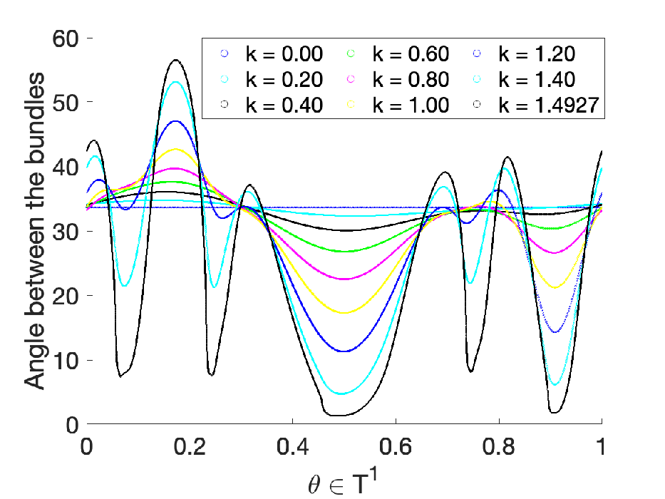
To quantify the separation between bundles, we measure the minimum angle between the invariant circle and the corresponding stable manifolds. Figure 10a indicates the angles for the $k$ values as in Figure 5. Figure 10b plots the minimum angle with respect to $k$ , and Figure 10c plots the corresponding $\theta\in\mathbb{T}$ such that the minimum angle is reached.

As indicated in Figure 10b, the slope of the blue curve (minimum angle) is approaching negative infinity (it is not obvious in the plot due to the different scales in the horizontal and vertical axis). As a matter of fact, the later portion of the minimum angle curve can be fitted by the following asymptotic expression using nonlinear regression:

(30)

\alpha(k-k_{crit})^{\beta},

where $\alpha$ is the scaling constant, $\beta$ is the scaling exponent, and $k_{crit}$ is the breakdown threshold. In fact, $\alpha=45.8879$ , $\beta=0.9085$ and $k_{crit}=1.5247$ gives us an estimation for the critical value such that the tangent and normal bundle collapse.

Remark 35.

The asymptotic expression (30) appears in [CC10] when it comes to estimating the blow-up of the Sobolev norm of the parameterization of the invariant circle. Empirically, Figure 10b shows that the minimum angle also approaches 0 following such power laws with universal exponents.

Since the rotation number in this example is not prescribed, it may change along the continuation. In our example, the change of the rotation number as $k$ increases is presented in Figure 10d.

Remark 36.

Note that the continuous family of orientation-preserving circle homeomorphism $a_{k}$ is not monotone, in the sense that the lift of $a_{k}$ can not be compared universally on $\mathbb{T}$ [KH95], thus the rotation number in Figure 10d is not expected to be monotone.

Remark 37.

We are still expecting “stairs” (intervals for $k$ in which case the rotation number is rational). In Figure 10d, the only obvious one is when the rotation number is $0.4$ , while the rest of the “stairs” (for example, corresponding to rotation number $0.3999$ ) is too small to be spotted.

As indicated in Figure 10d, the rotation number is rational when $k>1.3712$ . In this region, as discussed in Section 6.1.4, there are two periodic orbit, the attractive one with eigenvalues $\lambda^{s},\mu^{s}$ , and the hyperbolic one with eigenvalues $\lambda^{u},\mu^{u}$ . In Figure 10e, one can see how the eigenvalue changes as $k$ increases, as well as how the regularity $r^{*}$ (as discussed in Section 6.1.4) changes. The separation between $\lambda^{s}$ and $\mu^{s}$ indicates that the contraction rate in the tangential and normal direction will never meet in this example. Figure 10f present the eigenvectors on each periodic point.

Remark 38.

[HdlL07] has explored the bundle-merging phenomenon for quasi-periodic maps. Here, we have seen that a similar phenomenon happens for families in which the circles in the family alternate between phase-locked and rotational. Some quantitative aspects of the phenomenon can be different.

7. Numerical algorithm in 3-D maps

In this section, we further generalize our algorithm to three-dimensional maps which possesses one-dimensional invariant circles.

Following the same idea introduced previously, we first briefly discuss the derivation of the algorithm, and then implement such algorithm to the 3-dimensional Fattened Arnold Family (3D-FAF) maps.

7.1. Basic Derivation of the Algorithm

Given a map $f:\mathbb{T}^{1}\times\mathbb{R}^{2}\rightarrow\mathbb{T}^{1}\times\mathbb{R}^{2}$ that induces a one-dimensional invariant circle, the goal in this subsection is to derive an algorithm computing both the invariant circle and the corresponding isochrons.

Because of the increase of dimension on the isochrons, the analogue of invariance equation (2) is:

(31)

f\circ W(\theta,s_{1},s_{2})=W(a(\theta),\lambda_{1}(\theta)s,\lambda_{2}(\theta)s),

where $W:\mathbb{T}^{1}\times\mathbb{R}^{2}\rightarrow\mathbb{T}^{1}\times\mathbb{R}^{2}$ , $a:\mathbb{T}^{1}\rightarrow\mathbb{T}^{1}$ , $\lambda_{1}:\mathbb{T}^{1}\rightarrow\mathbb{T}^{1}$ and $\lambda_{2}:\mathbb{T}^{1}\rightarrow\mathbb{T}^{1}$ are the unknowns. Again, $a$ is the internal dynamics on the invariant circle, and for any given $\theta_{0}\in\mathbb{T}$ , $W(\theta_{0},s_{1},s_{2})$ parameterizes the isochron, $\lambda_{1}(\theta_{0})s_{1},\lambda_{2}(\theta_{0})s_{2}$ are the dynamics on the isochron along the eigen-directions.

Following the same procedure as in Section 2, we are looking for $\Delta_{a}(\theta)$ , $\Delta_{\lambda_{1}}(\theta)$ , $\Delta_{\lambda_{2}}(\theta)$ and $\Delta_{W}(\theta,s_{1},s_{2})=DW(\theta,s_{1},s_{2})\Gamma(\theta,s_{1},s_{2})$ satisfing the following three equations:

(32)

Da(\theta)\Gamma_{1}(\theta,s_{1},s_{2})-\Delta_{a}(\theta)-\Gamma_{1}(a(\theta),\lambda_{1}(\theta)s_{1},\lambda_{2}(\theta)s_{2})=M_{1}(\theta,s_{1},s_{2}),

(33)

\lambda_{1}(\theta)\Gamma_{2}(\theta,s_{1},s_{2})-\Delta_{\lambda_{1}}(\theta)s_{1}-\Gamma_{2}(a(\theta),\lambda_{1}(\theta)s_{1},\lambda_{2}(\theta)s_{2})=M_{2}(\theta,s_{1},s_{2}),

(34)

\lambda_{2}(\theta)\Gamma_{3}(\theta,s_{1},s_{2})-\Delta_{\lambda_{2}}(\theta)s_{2}-\Gamma_{3}(a(\theta),\lambda_{1}(\theta)s_{1},\lambda_{2}(\theta)s_{2})=M_{3}(\theta,s_{1},s_{2}),

where

M(\theta,s_{1},s_{2})=\widetilde{e}(\theta,s_{1},s_{2})-\begin{pmatrix}0\\ D\lambda_{1}(\theta)s_{1}\Gamma_{1}(\theta,s_{1},s_{2})\\ D\lambda_{2}(\theta)s_{1}\Gamma_{1}(\theta,s_{1},s_{2})\end{pmatrix},

and

\widetilde{e}(\theta,s_{1},s_{2})=-[DW(a(\theta),\lambda_{1}(\theta)s_{1},\lambda_{2}(\theta)s_{2})]^{-1}e(\theta,s_{1},s_{2}).

By discretizing function $g$ with three variables $(\theta,s_{1},s_{2})$ as

(35)

g(\theta,s_{1},s_{2})=\sum_{x=0}^{\infty}\sum_{y=0}^{\infty}g^{(x,y)}(\theta)s_{1}^{x}s_{2}^{y},

we again can further discritize Equation (32), (33) and (34) order by order as follows:

•

Equation (32):

–

Order $(0,0)$ :

(36)

Da(\theta)\Gamma_{1}^{(0,0)}(\theta)-\Delta a(\theta)-\Gamma_{1}^{(0,0)}(a(\theta))=M_{1}^{(0,0)}(\theta),

–

Order $(x,y)$ :

(37)

\Gamma_{1}^{(x,y)}(\theta)=\frac{\lambda_{1}^{x}(\theta)\lambda_{2}^{y}(\theta)}{Da(\theta)}\Gamma_{1}^{(x,y)}(a(\theta))+\frac{1}{Da(\theta)}M_{1}^{(x,y)}(\theta)

•

Equation (33):

–

Order $(0,0)$ :

(38) $\lambda_{1}(\theta)\Gamma_{2}^{(0,0)}(\theta)-\Gamma_{2}^{(0,0)}(a(\theta))=M_{2}^{(0,0)}(\theta),$

–

Order $(1,0)$ :

(39)

\lambda_{1}(\theta)\Gamma_{2}^{(1,0)}(\theta)-\Delta_{\lambda_{1}}(\theta)-\Gamma_{2}^{(1,0)}(a(\theta))\lambda_{1}(\theta)=M_{2}^{(1,0)}(\theta),

–

Order $(x,y)$ :

(40)

\Gamma_{2}^{(x,y)}(\theta)=\lambda_{1}^{x-1}(\theta)\lambda_{2}^{y}(\theta)\Gamma_{2}^{(x,y)}(a(\theta))+\frac{M_{2}^{(x,y)}(\theta)}{\lambda_{1}(\theta)},

•

Equation (34):

–

Order $(0,0)$ :

(41) $\lambda_{2}(\theta)\Gamma_{3}^{(0,0)}(\theta)-\Gamma_{3}^{(0,0)}(a(\theta))=M_{3}^{(0,0)}(\theta),$

–

Order $(0,1)$ :

(42)

\lambda_{2}(\theta)\Gamma_{3}^{(1,0)}(\theta)-\Delta_{\lambda_{2}}(\theta)-\Gamma_{3}^{(1,0)}(a(\theta))\lambda_{2}(\theta)=M_{3}^{(1,0)}(\theta),

–

Order $(x,y)$ :

(43)

\Gamma_{3}^{(x,y)}(\theta)=\lambda_{1}^{x}(\theta)\lambda_{2}^{y-1}(\theta)\Gamma_{3}^{(x,y)}(a(\theta))+\frac{M_{3}^{(x,y)}(\theta)}{\lambda_{2}(\theta)}.

Equations (36), (39) and (42) are underdetermined equations that can be solved by letting

\Gamma_{1}^{(0,0)}(\theta)=\Gamma_{2}^{(1,0)}(\theta)=\Gamma_{3}^{(0,1)}(\theta)=0,

and thus $\Delta_{a}(\theta)=-M^{(0,0)}(\theta)$ , $\Delta_{\lambda_{1}}(\theta)=-M^{(1,0)}(\theta)$ and $\Delta_{\lambda_{2}}(\theta)=-M^{(0,1)}(\theta)$ .

Equations (37), (38), (40), (41), (43) can be written in the format

\phi(\theta)=l(\theta)\phi(a(\theta))+\eta(\theta),

if the dynamical average $l^{*}<1$ (Remark 7), or be rewritten in the format

\phi(\theta)=\frac{1}{l(a^{-1})(\theta)}\phi(a^{-1}(\theta))-\frac{\eta(a^{-1}(\theta))}{l(a^{-1}(\theta))},

if $(\frac{1}{l(a^{-1})})^{*}<1$ , and such equations can then be solved through contraction as in (2.2.2) and Algorithm 2.

Remark 39.

In the 3-dim case, our quasi-Newton method does not work if $\lambda_{1}(\theta)$ and $\lambda_{2}(\theta)$ are resonant.

In fact, in this case, the fibered version of the Sternberg theorem fails. We are expecting a fibered version of Chen’s Theorem [Che63]. More specifically, for $|\lambda_{2}|^{q}<|\lambda_{1}|$ , we are expecting a polynomial $p(\theta,s)$ with degree $\leq q$ such that the invariance equation becomes

f(W(\theta,s))-W(a(\theta),p(\theta,s))=0.

The same discussions remain valid for higher-dimensional cases. We hope to come back to this problem and develop a complete theory.

7.2. Numerical Exploration: 3D-Fattened Arnold Family

Inspired by [HCF+16], in this subsection, we implement the algorithm discussed in Section 7.1 on a 3-dimensional Fattened Arnold Family (3D-FAF) $f_{\alpha,\epsilon}:\mathbb{T}^{1}\times\mathbb{R}^{2}\rightarrow\mathbb{T}^{1}\times\mathbb{R}^{2}$ :

(44)

f_{\alpha,\epsilon}(x,y,z)=\begin{pmatrix}x+\alpha+\frac{\epsilon}{2\pi}(\sin(2\pi x)+y+\frac{z}{2})\\ \beta(\sin(2\pi x)+y)\\ \gamma(\sin(2\pi x)+y+z)\end{pmatrix},

where $\epsilon$ is the perturbation parameter, $\alpha$ is the drift parameter and $\beta$ , $\gamma$ are the eigenvalues. We have implemented the algorithm for the stable (i.e. $\beta<1$ , $\gamma<1$ ) case, unstable ( $\beta>1$ , $\gamma>1$ ) case and the saddle (i.e. $\beta<1<\gamma$ ) case.

7.2.1. The Unperturbed Case

In order to apply the continuation method, we start with the unperturbed case where $\epsilon=0$ . As discussed in [HCF+16], in such case, the solution to the invariance equation (31) is:

	$\displaystyle W_{1}(\theta,s_{1},s_{2})$	$\displaystyle=\theta,$
	$\displaystyle W_{2}(\theta,s_{1},s_{2})$	$\displaystyle=-S(\alpha,\beta)\cos(2\pi\theta)+(C(\alpha,\beta)-1)\sin(2\pi\theta)+s_{1},$
	$\displaystyle W_{3}(\theta,s_{1},s_{2})$	$\displaystyle=\frac{\gamma}{\beta}\big(S(\alpha,\beta)(C(-\alpha,\gamma^{-1})-1)+(C(\alpha,\beta)-1)S(-\alpha,\gamma^{-1})\big)\cos(2\pi\theta)$
		$\displaystyle\ \ \ \frac{\gamma}{\beta}\big((C(\alpha,\beta)-1)(C(-\alpha,\gamma^{-1})-1)-S(\alpha,\beta)S(-\alpha,\gamma^{-1})\big)\sin(2\pi\theta)$
		$\displaystyle\ \ \ +\frac{\gamma}{\beta-\gamma}s_{1}+s_{2},$
	$\displaystyle a(\theta)=\theta+\alpha$	$\displaystyle,\text{ }\lambda_{1}(\theta)=\beta,\text{ }\lambda_{2}(\theta)=\gamma,$

where

S(x,y)=\frac{y\sin(2\pi x)}{1-2y\cos(2\pi x)+y^{2}},\ C(x,y)=\frac{1-y\cos(2\pi x)}{1-2y\cos(2\pi x)+y^{2}}.

7.2.2. The Perturbed Case

Following the same continuation method as in Section 4, the invariant circle and the corresponding isochrons are computed for all the stable, unstable, and saddle choice of the parameters. For the same color choice as in Figure 2a, we still start with the blue isochron, which is mapped to the green isochron, followed by magenta, cyan, and black, correspondingly (see Figure 11, 12 and 13).

Appendix A A Proposal for a Parallel Implementation of the Algorithm: a Digression

Although the parallelization is not implemented in this paper, we remark that Algorithm 1 can be parallelized using a 2-dimensional mesh of processors as the communication network. In this Appendix, we propose a draft framework when multiple processors are available.

This subsection is a digression from the main argument of the paper and we have not implemented the algorithms discussed here. It can be omitted without affecting the rest.

A two-dimensional communication network (with no wraparound link) is an embedding network in the way that the processors are arranged to a matrix, where each processor can communicate with their nearest neighbors in the same row or column. This type of embedding is commonly used in matrix manipulation.

A.1. Function Representation in 2-dim Network

In our algorithm, the functions we are dealing with are either of Type-1 (see Section 3.1): i.e. $a(\theta),\lambda(\theta)$ , which are stored as a 1-D array, or of Type-2: i.e. $W(\theta,s)$ , which is stored as a matrix of size $N\times(L+1)$ . We can block distribute Type-1 functions onto the first row of the grid, and block distribute Type-2 functions on the 2-D grid.

More precisely, suppose the 2-D network has size $P_{N}\times P_{L}$ , and $N,L$ are integer multiples of $P_{N},P_{L}$ , respectively, then each processor on the first row stores $\frac{N}{P_{N}}$ points for functions of Type-1, and each processor stores $\frac{N}{P_{N}}\times\frac{L}{P_{L}}$ points for functions of Type-2.

Storing functions blockwise in this way allows the basic functional operations (for example, summation, subtractions, Type-1 function multiplication) to be processed within each processor in a pointwise manner without communication. The delicate part is the operations when communications between processors are needed. In our algorithm, such operations include function evaluation (for composition) and Taylor polynomial multiplication.

A.2. Cubic Spline Interpolation in Parallel

Interpolations are required in our algorithm whenever composition between functions or derivatives of functions are needed. Because of the way functions are stored, cubic spline interpolations need to be performed on each row of the communication network.

The computation for the coefficients of cubic splines is essentially achieved by solving a linear system, where the matrix involved is only a tridiagonal matrix. Thus the goal is to solve this tridiagonal system on a 1-D network.

Following [MRKK16], such system can be reduced to a single variable equation recursively in $\log_{3}N$ steps, which, when implemented parallelly, has time complexity $\mathcal{O}((\tau+\mu)\log P_{N})$ (for communication) and $\mathcal{O}(\log\frac{N}{P_{N}})$ (for computation), where $\tau$ is the latency time, $\mu$ is the inverse of the bandwidth, and $m$ is the size of the message communicating between processors (in this case is just a constant). Pipelining techniques [MM11] can be used to speedup this computation.

To perform composition, we need to first use the hypercubic AllGather technique to have all the processors in the same row gather all the pieces of the spline (with communication time complexity $\mathcal{O}(\tau\log P_{N}+\mu N)$ ). For example, when computing $W(a(\theta),\lambda(\theta)s)$ , one need to first BroadCast every piece of $a(\theta)$ from the first row to the rest rows along the corresponding columns (with communication time complexity $\mathcal{O}((\tau+\mu)\log P_{N})$ ), compute $\lambda^{i}(\theta)$ for row $i$ using parallel prefix sum technique (with communication time $\mathcal{O}(\tau\log P_{L}+\mu\frac{N}{P_{N}}\log P_{L})$ and computation time $\mathcal{O}(\frac{L\times N}{P_{L}\times P_{N}}+\frac{N}{P_{N}}\log P_{L})$ ), perform the interpolation for each row for the corresponding $W^{(i)}(\theta)$ , $i=0,\dots,L$ , AllGather the spline on each processor, and then evaluate on $a(\theta)$ , and then multiply it by the corresponding $\lambda^{i}(\theta)$ pointwisely.

A.3. Type-2 Function Multiplication in Parallel

In our algorithm, products between Type-2 functions are also required. Given $g_{1}(\theta,s)=\sum_{i=0}^{L}g_{1}^{(i)}(\theta)s^{i}$ , $g_{2}(\theta,s)=\sum_{i=0}^{L}g_{2}^{(i)}(\theta)s^{i}$ , we need to compute $g_{1}\times g_{2}$ up to the $L$ -th order. To achieve this, one can AllGather $g_{2}$ for each column, compute the corresponding coefficients, and then AllReduce (with time complexity $\mathcal{O}(\tau\log P_{L})+\mu\frac{N}{P_{N}}\log P_{L}$ ) along each column to update the coefficients for the product.

References

[BS08] Kristian Bjerklöv and Maria Saprykina. Universal asymptotics in hyperbolicity breakdown. Nonlinearity, 21(3):557–586, 2008.
[BST98] Henk Broer, Carles Simó, and Joan Carles Tatjer. Towards global models near homoclinic tangencies of dissipative diffeomorphisms. Nonlinearity, 11(3):667–770, 1998.
[CC10] Renato Calleja and Alessandra Celletti. Breakdown of invariant attractors for the dissipative standard map. Chaos, 20(1):013121, 9, 2010.
[CCdlL13] Renato C. Calleja, Alessandra Celletti, and Rafael de la Llave. A KAM theory for conformally symplectic systems: efficient algorithms and their validation. J. Differential Equations, 255(5):978–1049, 2013.
[CF12] Renato Calleja and Jordi-Lluís Figueras. Collision of invariant bundles of quasi-periodic attractors in the dissipative standard map. Chaos, 22(3):033114, 10, 2012.
[CFdlL03] Xavier Cabré, Ernest Fontich, and Rafael de la Llave. The parameterization method for invariant manifolds. I. Manifolds associated to non-resonant subspaces. Indiana Univ. Math. J., 52(2):283–328, 2003.
[CFdlL05] Xavier Cabré, Ernest Fontich, and Rafael de la Llave. The parameterization method for invariant manifolds. III. Overview and applications. J. Differential Equations, 218(2):444–515, 2005.
[CH17a] Marta Canadell and Àlex Haro. Computation of quasi-periodic normally hyperbolic invariant tori: algorithms, numerical explorations and mechanisms of breakdown. J. Nonlinear Sci., 27(6):1829–1868, 2017.
[CH17b] Marta Canadell and Àlex Haro. Computation of quasiperiodic normally hyperbolic invariant tori: rigorous results. J. Nonlinear Sci., 27(6):1869–1904, 2017.
[Che63] Kuo-Tsai Chen. Equivalence and decomposition of vector fields about an elementary critical point. Amer. J. Math., 85:693–722, 1963.
[CI79a] A. Chenciner and G. Iooss. Bifurcations de tores invariants. Arch. Rational Mech. Anal., 69(2):109–198, 1979.
[CI79b] A. Chenciner and G. Iooss. Persistance et bifurcation de tores invariants. Arch. Rational Mech. Anal., 71(4):301–306, 1979.
[CJ15] Y.-M. Chung and M. S. Jolly. A unified approach to compute foliations, inertial manifolds, and tracking solutions. Math. Comp., 84(294):1729–1751, 2015.
[CK20] Maciej J. Capiński and Hieronim Kubica. Persistence of normally hyperbolic invariant manifolds in the absence of rate conditions. Nonlinearity, 33(9):4967–5005, 2020.
[dlL97] Rafael de la Llave. Invariant manifolds associated to nonresonant spectral subspaces. J. Statist. Phys., 87(1-2):211–249, 1997.
[dlL03] R. de la Llave. Invariant manifolds associated to invariant subspaces without invariant complements: a graph transform approach. Math. Phys. Electron. J., 9:Paper 3, 35, 2003.
[DSSY16] Suddhasattwa Das, Yoshitaka Saiki, Evelyn Sander, and James Yorke. Quasiperiodicity: Rotation Numbers, Proceeding of The Foundations of Chaos Revisited: From Poincare to Recent Advancements, Chapter 7. Springer Complexity, Switzerland, 2016.
[DSSY19] Suddhasattwa Das, Yoshitaka Saiki, Evelyn Sander, and James A. Yorke. Solving the Babylonian problem of quasiperiodic rotation rates. Discrete Contin. Dyn. Syst. Ser. S, 12(8):2279–2305, 2019.
[ER85] J.-P. Eckmann and D. Ruelle. Ergodic theory of chaos and strange attractors. Rev. Modern Phys., 57(3, part 1):617–656, 1985.
[Fen72] Neil Fenichel. Persistence and smoothness of invariant manifolds for flows. Indiana Univ. Math. J., 21:193–226, 1971/72.
[Fen74] Neil Fenichel. Asymptotic stability with rate conditions. Indiana Univ. Math. J., 23:1109–1137, 1973/74.
[FH13] Jordi-Lluís Figueras and Àlex Haro. Triple collisions of invariant bundles. Discrete Contin. Dyn. Syst. Ser. B, 18(8):2069–2082, 2013.
[FH15] Jordi-Lluís Figueras and Àlex Haro. Different scenarios for hyperbolicity breakdown in quasiperiodic area preserving twist maps. Chaos, 25(12):123119, 16, 2015.
[GYdlL21] Joan Gimeno, Jiaqi Yang, and Rafael de la Llave. Numerical computation of periodic orbits and isochrons for state-dependent delay perturbation of an ODE in the plane. SIADS, 20, 2021. To appear.
[HCF+16] Àlex Haro, Marta Canadell, Jordi-Lluís Figueras, Alejandro Luque, and Josep-Maria Mondelo. The parameterization method for invariant manifolds, volume 195 of Applied Mathematical Sciences. Springer, [Cham], 2016. From rigorous results to effective computations.
[HdlL07] A. Haro and R. de la Llave. A parameterization method for the computation of invariant tori and their whiskers in quasi-periodic maps: explorations and mechanisms for the breakdown of hyperbolicity. SIAM J. Appl. Dyn. Syst., 6(1):142–207, 2007.
[HdlL13] Gemma Huguet and Rafael de la Llave. Computation of limit cycles and their isochrons: fast algorithms and their convergence. SIAM J. Appl. Dyn. Syst., 12(4):1763–1802, 2013.
[HdlLS13] Gemma Huguet, Rafael de la Llave, and Yannick Sire. Fast iteration of cocycles over rotations and computation of hyperbolic bundles. Discrete Contin. Dyn. Syst., (Dynamical systems, differential equations and applications. 9th AIMS Conference. Suppl.):323–333, 2013.
[HM76] Charles A. Hall and W. Weston Meyer. Optimal error bounds for cubic spline interpolation. J. Approximation Theory, 16(2):105–122, 1976.
[HPS77] M. W. Hirsch, C. C. Pugh, and M. Shub. Invariant manifolds. Lecture Notes in Mathematics, Vol. 583. Springer-Verlag, Berlin-New York, 1977.
[JK69] Jiří Jarník and Jaroslav Kurzweil. On invariant sets and invariant manifolds of differential systems. J. Differential Equations, 6:247–263, 1969.
[KH95] Anatole Katok and Boris Hasselblatt. Introduction to the modern theory of dynamical systems, volume 54 of Encyclopedia of Mathematics and its Applications. Cambridge University Press, Cambridge, 1995. With a supplementary chapter by Katok and Leonardo Mendoza.
[Knu98] Donald E. Knuth. The art of computer programming. Vol. 2. Addison-Wesley, Reading, MA, 1998. Seminumerical algorithms, Third edition [of MR0286318].
[Kre78] Ulrich Krengel. On the speed of convergence in the ergodic theorem. Monatshefte für Mathematik, 86(1):3–6, 1978.
[Lev81] Mark Levi. Qualitative analysis of the periodically forced relaxation oscillations. Mem. Amer. Math. Soc., 32(244):vi+147, 1981.
[LKO14] Peter Langfield, Bernd Krauskopf, and Hinke M. Osinga. Solving Winfree’s puzzle: the isochrons in the FitzHugh-Nagumo model. Chaos, 24(1):013131, 13, 2014.
[Los88] Jérôme E. Los. Dédoublement de courbes invariantes sur le cylindre: petits diviseurs. Ann. Inst. H. Poincaré Anal. Non Linéaire, 5(1):37–95, 1988.
[MM11] Panagiotis D. Michailidis and Konstantinos G. Margaritis. Parallel direct methods for solving the system of linear equations with pipelining on a multicore using openmp. Journal of Computational and Applied Mathematics, 236(3):326–341, 2011. Aspects of Numerical Algorithms, Parallelization and Applications.
[Mn78] Ricardo Mañé. Persistent manifolds are normally hyperbolic. Transactions of the American Mathematical Society, 246:261–283, 1978.
[MRKK16] Prasant Kumar Mohanty, Motahar Reza, Piyush Kumar, and Praveen Kumar. Implementation of cubic spline interpolation on parallel skeleton using pipeline model on cpu-gpu cluster. In 2016 IEEE 6th International Conference on Advanced Computing (IACC), pages 747–751. IEEE, 2016.
[OT17] Thomas Ohlson Timoudas. Power law asymptotics in the creation of strange attractors in the quasi-periodically forced quadratic family. Nonlinearity, 30(12):4483–4522, 2017.
[Pal08] J. Palis. Open questions leading to a global perspective in dynamics. Nonlinearity, 21(4):T37–T43, 2008.
[Pes04] Yakov B. Pesin. Lectures on partial hyperbolicity and stable ergodicity. Zurich Lectures in Advanced Mathematics. European Mathematical Society (EMS), Zürich, 2004.
[Ran92a] D. A. Rand. Existence, nonexistence and universal breakdown of dissipative golden invariant tori. I. Golden critical circle maps. Nonlinearity, 5(3):639–662, 1992.
[Ran92b] D. A. Rand. Existence, nonexistence and universal breakdown of dissipative golden invariant tori. II. Convergence of renormalization for mappings of the annulus. Nonlinearity, 5(3):663–680, 1992.
[Ran92c] D. A. Rand. Existence, nonexistence and universal breakdown of dissipative golden invariant tori. III. Invariant circles for mappings of the annulus. Nonlinearity, 5(3):681–706, 1992.
[Sel79] George R. Sell. Bifurcation of higher-dimensional tori. Arch. Rational Mech. Anal., 69(3):199–230, 1979.
[Ste90] M. Steffen. A simple method for monotonic interpolation in one dimension. Astronomy and Astrophysics, 239:443–450, 1990.
[Win75] A. T. Winfree. Patterns of phase compromise in biological cycles. J. Math. Biol., 1(1):73–95, 1974/75.
[WY01] Qiudong Wang and Lai-Sang Young. Strange attractors with one direction of instability. Comm. Math. Phys., 218(1):1–97, 2001.
[WY03] Qiudong Wang and Lai-Sang Young. Strange attractors in periodically-kicked limit cycles and Hopf bifurcations. Comm. Math. Phys., 240(3):509–529, 2003.
[YdlL21] Yian Yao and Rafael de la Llave. Algorithms for computation of attractors and isochrones for 2-d maps: Effective algorithms and rigorous proofs of convergence. 2021. Preprint.
[ZdlL18] Lei Zhang and Rafael de la Llave. Transition state theory with quasi-periodic forcing. Commun. Nonlinear Sci. Numer. Simul., 62:229–243, 2018.

COMPUTING THE INVARIANT CIRCLE AND THE FOLIATION BY STABLE MANIFOLDS FOR A 2-D MAP BY THE PARAMETERIZATION METHOD: NUMERICAL IMPLEMENTATION AND RESULTSThanks: Supported in part by NSF DMS-1800241

Abstract.

Key words and phrases:

2021 Mathematics Subject Classification

1. Introduction

1.1. Other results in the literature

1.2. Organization of the Paper

2. The Numerical Algorithm

2.1. The Invariance Equation

Remark 1.

Remark 2.

Remark 3.

Remark 4.

2.2. The quasi-Newton Method

2.2.1. Derivation of the Iterative Step

Remark 5.

2.2.2. Corrections of W⁡(θ,s),a⁡(θ),λ⁡(θ)W(\theta,s),a(\theta),\lambda(\theta)

Definition 1.

Remark 6.

2.2.1.1. Solving for Δa​(θ)\Delta_{a}(\theta) and Δλ​(θ)\Delta_{\lambda}(\theta):

2.2.1.2. Solve for Γ1(j)​(θ),j≠0\Gamma_{1}^{(j)}(\theta),j\neq 0 and Γ2(k)​(θ),j≠1\Gamma_{2}^{(k)}(\theta),j\neq 1:

Remark 7.

2.3. The Algorithm for One Iteration of the quasi-Newtons Method

Remark 8.

Remark 9.

3. Some Implementation Details

3.1. Function Representation

3.1.1. Type-1 Functions

Remark 10.

Remark 11.

3.1.2. Type-2 Functions

3.2. Composition Between Functions

3.2.1. Coping with Function Composition in CrC^{r}

Remark 12.

Remark 13.

Remark 14.

3.2.2. Coping with Function Composition in 𝒳r,δ\mathcal{X}^{r,\delta}

3.2.3. The Computation of e~​(θ,s)\widetilde{e}(\theta,s)

3.3. Computation of the Approximate Inverse of the Internal Dynamics

Remark 15.

3.4. A Fast Algorithm for Solving Cohomological Equations

Remark 16.

Remark 17.

Remark 18.

Remark 19.

Remark 20.

Remark 21.

3.5. Truncation Versus Smoothing Operator

3.6. Validation of the Correctness of the Solution

4. Continuation Method

4.1. The Continuation Method

4.1.1. Basic Idea

Remark 22.

4.1.2. The Continuation Algorithm

Remark 23.

4.1.3. Adaptative Grid for Continuation

Remark 24.

5. Numerical Explorations

Remark 25.

Remark 26.

Remark 27.

5.1. Example Solution

5.1.1. Convergence of the quasi-Newton Iteration

Remark 28.

Remark 29.

5.1.2. Validation for Correctness of the Solution

Remark 30.

5.1.3. Methods for Computing the Inverse of a⁡(θ)a(\theta)

Remark 31.

5.1.4. Run Time Analysis

5.1.5. Plot of the Invariant Circle and Isochrons

Remark 32.

5.1.6. Globalization

Remark 33.

Remark 34.

5.2. Continuation w.r.t. kk

5.3. Continuation w.r.t. η\eta

5.3.1. Computation of the Rotation Number

5.3.2. Distinguishing Irrational Rotations from Rational Rotations

5.4. Continuation with Prescribed Rotation Number

COMPUTING THE INVARIANT CIRCLE AND THE FOLIATION BY STABLE MANIFOLDS FOR A 2-D MAP BY THE PARAMETERIZATION METHOD:
NUMERICAL IMPLEMENTATION AND RESULTSThanks: Supported in part by NSF DMS-1800241

2.2.2. Corrections of $W(\theta,s),a(\theta),\lambda(\theta)$

2.2.1.1. Solving for $\Delta_{a}(\theta)$ and $\Delta_{\lambda}(\theta)$ :

2.2.1.2. Solve for $\Gamma_{1}^{(j)}(\theta),j\neq 0$ and $\Gamma_{2}^{(k)}(\theta),j\neq 1$ :

3.2.1. Coping with Function Composition in $C^{r}$

3.2.2. Coping with Function Composition in $\mathcal{X}^{r,\delta}$

3.2.3. The Computation of $\widetilde{e}(\theta,s)$

5.1.3. Methods for Computing the Inverse of $a(\theta)$

5.2. Continuation w.r.t. $k$

5.3. Continuation w.r.t. $\eta$