Breakdown of light transport models in photonic scattering slabs with strong absorption and anisotropy
Abstract
The radiative transfer equation (RTE) models the transport of light inside photonic scattering samples such as paint, foam and tissue. Analytic approximations to solve the RTE fail for samples with strong absorption and dominant anisotropic scattering and predict unphysical negative energy densities and the diffuse flux in the wrong direction. Here we fully characterize the unphysical regions of three popular approximations to the RTE for a slab, namely the approximation (or diffusion approximation), the approximation, and a popular modification to that corrects the forward scattering in the approximation. We find that the delta function correction to eliminates the unphysical range in the forward scattering. In addition, we compare the predictions of these analytical methods to exact Monte Carlo simulations for the physical and unphysical regions. We present maps of relative errors for the albedo and the anisotropy of the scatterers for a realistic index contrast typical of a polymer slab in air and optical thickness. The relative error maps provide a guideline for the accuracy of the analytical methods to interpret experiments on light transport in photonic scattering slabs. Our results show that the approximation is significantly inaccurate to extract transport parameters unless the sample scatters purely isotropic and elastic. The approximation exceeds in terms of accuracy in its physical range for moderate absorption, and the with the delta function correction is the most accurate approximation considered here for the forward direction.
I Introduction
In photonic scattering media, such as paint, foam and tissue, the refractive index varies spatially causing incident waves to be scattered and absorbed Ishimaru 1978; van Rossum and Nieuwenhuizen 1999; Akkermans and Montambaux 2007; Wiersma 2013; Vos et al. 2015; Carminati and Schotland 2021. Understanding the transport of light in such scattering media is crucial for many application areas, such as atmospheric and climate sciences Fournier and Forand 1994; Fell and Fischer 2001; Stramski et al. 2004; Nousiainen and Kandler 2015, oceanography Funk 1973; McCormick 2006, biophysics Star 1989; Wilson and Jacques 1990; Cheong et al. 1990; Kienle and Hibst 2006, powder technology Sekulic et al. 1996; Burger et al. 1997, and solid-state lighting Schubert 2006; Krames et al. 2007; Bechtel et al. 2008; Meretska et al. 2019a. The transport theory describes the propagation of wave in scattering media, notably in a widely-used realistic situation like a slab in three dimensions (3D), as shown in Fig. 1(a). The theory describes the transfer of intensity and neglects interference effects including diffraction Ishimaru 1978. For all practical purposes the transport theory is rigorous and only in exceptional cases such as the situations of very strong elastic scattering and Anderson localization of light where interference predominates, the transport shows features beyond the predictions of transport theory van Rossum and Nieuwenhuizen 1999.
The basic differential equation used in transport theory is the radiative transfer equation (RTE), which is equivalent to Boltzmann’s equation used in the kinetic theory of gases and neutron transport Ishimaru 1978; Chandrasekhar 1960; Tait 1964. The most fundamental quantity is the specific intensity that describes the average power flux density at position in a given direction within a unit solid angle and a unit frequency band Ishimaru 1978. Due to its dependency on both the position and the direction , it is challenging to solve directly.
The most popular method to solve the RTE for light is the Monte Carlo simulation of light transport Prahl et al. 1989; Mujumdar et al. 2010; Jacques 2011; Atif et al. 2011; Uppu and Mujumdar 2013; Leino et al. 2019; Jönsson and Berrocal 2020; Cooper et al. 2021; Krieger and Wolf 2021, a statistical method that converges to the exact solution of the RTE. To obtain a high accuracy, however, this method comes with the cost of extremely long computation times Shonkwiler and Mendivil 2009, high computational power requirements with concomitant high energy consumption.
The complexity of transport theory and the tedious resource-consuming Monte Carlo simulations have stimulated the development of analytical approximations to the RTE Joseph et al. 1976; Star et al. 1988; Keijzer et al. 1988; Dickey et al. 1998; Liemert and Kienle 2011; Liemert et al. 2021. These analytical approximations are sustainable alternatives to Monte Carlo simulations, since computations consume much less resources. In addition, despite impressive advances made by graphics processing unit (GPU) based Monte Carlo simulations in terms of speed Leino et al. 2019; Jönsson and Berrocal 2020, analytical methods are significantly faster. Moreover, in certain configurations, such as the slab geometry, the results of these analytical approximations match the accuracy of simulations.
A widely used analytical approximation to the RTE is the approximation (See Appendix A for full solution for a slab geometry), where the dependence on both variables is separated Tait 1964 by expanding the specific intensity in products of complete sets on the domains of and
| (1) |
Here, are the spatial components, are the Laplace spherical harmonics Jackson 1998; Arfken and Weber 2005, and is the order of the approximation that determines the number of terms in Eq. (1). The analytical approximations are mostly used for simple sample geometries such as a slab and a sphere, and their accuracies depend notably on (i) the order of the approximation and (ii) on the optical properties of the medium. As approaches infinity, the approximation yields exact solutions. In realistic cases, such as a 3D slab, the order is rarely higher than as the mathematical complexity increases rapidly with increasing and becomes computationally demanding. 11 1 Odd positive integers are chosen for since odd order approximations are known to be more accurate than even orders, as in the latter the angular integrands are discontinuous Case and Zweifel 1967. In this work, we thoroughly validate the and approximations for a slab geometry Ext.

The first-order analytical approximation to transport theory is the diffusion theory Ishimaru 1978, which is widely used to extract transport parameters from opaque media with isotropic scatterers (see Fig. 1(b)) and with negligible absorption. For a slab shown in Fig. 1(a), this opaque configuration amounts to the thickness being much larger than the transport mean free path and much smaller than the absorption mean free path :
| (2) |
If the scattering is dominantly in the forward direction, increases (see Fig. 1(c)), and decreases if the scatterers have significant absorption (see Fig. 1(d)). Meretska et al. Meretska et al. 2019b defined a physically more informative validity range using the three-parameter space (,,) spanned by the albedo , the anisotropy , and the optical thickness . A practically relevant parameter space also requires consideration of the internal reflection at the slab boundaries Lagendijk et al. 1989; Zhu et al. 1991, so we add as a 4th parameter the refractive index contrast
| (3) |
Here, and are the refractive index of the medium inside the slab that surrounds the scatterers and the index of the medium outside the slab (typically free space), respectively. Once the (,,,) parameter set is known, the solution of approximation is fully determined.
In some parts of the (,,,) parameter space, the approximations predict unphysical behavior, such as a negative energy density. We call these regions unphysical ranges. An example of an unphysical result of the approximation is shown in Fig. 2(C,D). In Fig. 2(D) the diffusion theory predicts an unphysical negative energy density. The diffuse flux given in Fig. 2(C) is unphysical, since the theory predicts erroneously an incident diffuse flux , whereas a reflected flux opposite to the incident direction of light is required at the incident boundary (left boundary in Fig. 2).

In this paper, we map the unphysical ranges and the relative errors of three popular approximations to the RTE, namely, the , the , and the approximations. The approximation is a widely used higher-order approximation to RTE Bayazitoglu and Higenyi 1979; Meretska et al. 2019a; Meretska et al. 2017; Liemert and Kienle 2014, especially popular in biophysics Star 1989; Star et al. 1988; Dickey et al. 1998. The approximation uses a modified phase function within the approximation to increase the accuracy of the forward scattering region Star 1989; Star et al. 1988; Meador and Weaver 1979 (see Appendix B). The unphysical ranges of each approximation are found by scanning the (,,,) parameter space and looking for the regions where the conditions (4) are violated. In addition, the relative error maps are obtained by comparing the approximations to extensive Monte Carlo simulations. Our simulation code is based on the work of Prahl et al. Prahl et al. 1989, with the addition of multiple internal reflection similar to a Fabry-Pérot cavity Hecht 2016, where only the multiply reflected intensities are considered but no interference, see Ref. Bohren and Huffman 1998.
II Results & Discussions
II.1 The unphysical ranges
The physical validity conditions of the approximation are expressed mathematically as Meretska et al. 2019b:
| (4) |
Here is the average intensity that is directly proportional to the energy density Ishimaru 1978;
| (5) |
where is the speed of light. The unphysical ranges are found by checking whether the approximations violate one or more of the conditions given in equation (4), for each set of parameters(). The unphysical regions given in Figs. 3, 4 and 5 cover all possible albedos and anisotropies in photonic scattering slabs from backscattering to forward scattering. For all figures with anisotropy-albedo maps, the limits of anisotropy are and , and extreme absorption limit is . The perfect anisotropy ( and ) and perfect absorption () cases are not discussed here, as they are unphysical Olmos-Trigo et al. 2020; Kerker et al. 1983 and thus samples with such properties can not be realized. For similar reason van der Molen et al. 2006, we do not consider samples with gain.
Fig. 3 shows the unphysical ranges when the optical thickness and refractive index contrast are fixed (; , e.g., a polymer slab in air). The approximation, being the higher-order approximation, is generally believed to be an improvement on the approximation Star 1989. Hence we expected a shrinking of the unphysical range in going from to . In Fig. 3(b), however, the expected improvement is not observed. It is even more remarkable that parts of the physical regions of the approximation are unphysical for the . As expected, the approximation is entirely physical for the forward scattering region. In the dominant backscattering range around and below, however, the approximation is primarily unphysical even without absorption, which is also reasonable since the approximation is a modification to correct only the forward direction.

The effects of varying the thickness and the index contrast are presented in Fig. 4 and Fig. 5, respectively. Increasing the optical thickness from to (see Fig. 4) has more effect on the unphysical range of the approximation compared to the other methods. A clear increase is seen in the unphysical range of the approximation, from strong to weak absorption regions, and some minor expansion towards the isotropic regions with increased thickness . For the approximation, increasing also results in an expansion of the unphysical range, however, the change is smaller than in the approximation. In contrast, the unphysical range of the approximation remains almost the same for all thicknesses.


In Fig. 5 we show the unphysical ranges when the index contrast is varied up to at a fixed optical thickness (). As increases, the unphysical range of the approximation shrinks towards the non-absorbing region. Interestingly, for the approximation, the situation has a very small unphysical range in the extreme limits of the (,) plane. As the index contrast increases to , the unphysical range increases dramatically. However, a further increase to decreases the unphysical range. The unphysical ranges of the approximation are again invariant to changes in .
Our investigations of the unphysical ranges show that the approximation to the RTE should not be used for slabs with anisotropic scattering. The approximation seems to be especially good for samples with a refractive index matching with the medium outside, as it is physical almost everywhere. Nevertheless, detailed investigations (not shown here) of the approximation for show that there are significant relative errors in the dominant forward scattering range (). The approximation is found to be physical for the forward scattering region and invariant for the changes in and . It is, however, the worst approximation considered here for the backscattering region.
II.2 Evaluating relative errors
In practice, the transport mean free path and the absorption mean free path are extracted from total transmission and total reflection experiments using a approximation Meretska et al. 2017.
The unphysical ranges of a approximation are essential to recognize for which photonic scattering slabs that particular approximation should not be used for extracting these transport parameters.
However, the bare acknowledgement of the unphysical ranges do not give any information on the accuracy of these methods to interpret observations on samples residing in the physical regions.
Therefore, we extensively compare with Monte Carlo simulations to obtain relative error maps of transport parameters obtained by the analytical approximation methods.
The optical thickness and refractive index contrast are chosen to be ().

Comparisons are done on the basis of the observation of both the total transmission and total reflection that can come from a real experiment or from Monte Carlo simulations. The comparison takes four steps:
- 1.
We calculate and using Monte Carlo simulations, using a fine grid in parameter space : and . We compare these Monte Carlo results to the results obtained for all albedos and anisotropies, using the same fine grid in parameter space : and . We define the squared relative distance between the two results
(6) (7) We also define the overall relative distance between the two calculations
(8) - 2.
As a first impression of the errors, the results are compared by calculating relative errors Epperson 2013 for identical grid points and , defined by
(9) (10) An example of a comparison in this step corresponds to comparing the blue square I in the Monte Carlo grid with the red square II in the grid in Fig. 6. The relative error maps for all are shown in Fig. 7(a-f).
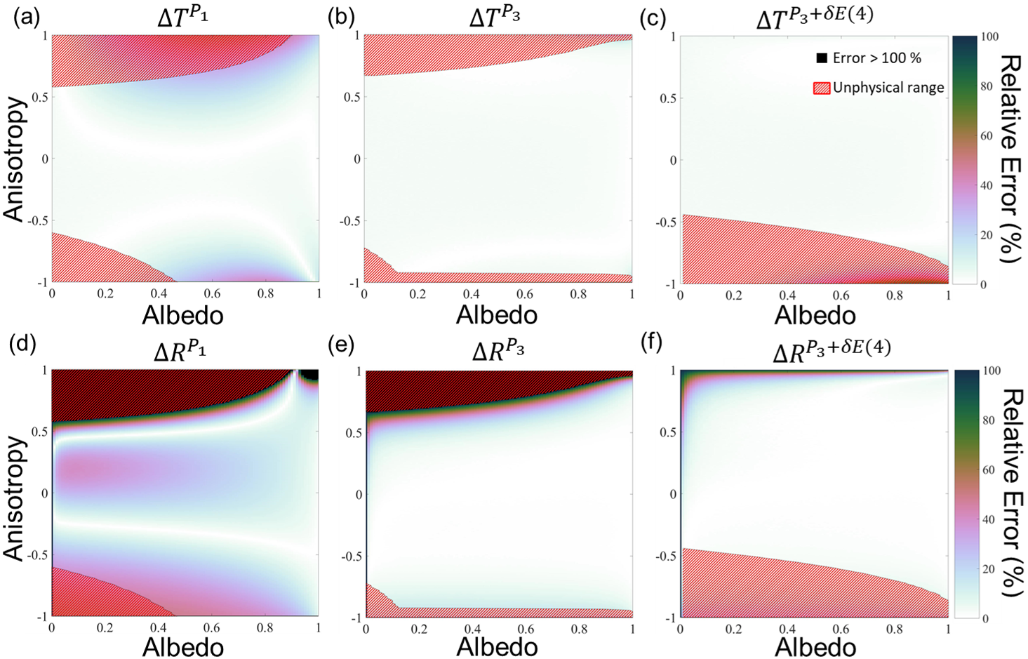
Figure 7: Relative error maps of the total transmission and the total reflection results for the approximations. (a) and (d) for , (b) and (e) for , (c) and (f) for . Relative errors reported here are calculated by comparing these approximations to our Monte Carlo simulations. Color map indicates the percentage of errors. Values that are larger than are indicated with black markers. The unphysical ranges of the approximations are added to the graphs as red hatched regions. Optical thickness and refractive index contrast are specifically chosen as and for these relative error maps. - 3.
In a real experiment, one measures the total transmission T and the total reflection R of a sample and uses a numerical or an analytical method to infer the parameters that corresponds to the observations. In this work we take T and R from Monte Carlo simulations as they are highly accurate (see Table 1). We call the set obtained from Monte Carlo simulations , from which we infer the true transport lengths, and . If we interpret the Monte Carlo T and R results with the approximation, we obtain the parameter set called , that minimizes the distance . From the matched pair we infer the mean free paths and of that sample using the appropriate approximation. This step is illustrated in Fig. 6 where the blue grid point III in the grid represents (,) pair fitted to the blue grid point I in the Monte Carlo grid.
- 4.
In the final step, the procedure of the previous step is repeated for all possible (,) and its matched pair (), and we calculate the relative errors of the interpretations of the analytic approximation:
(11) (12) These results are plotted in Fig. 8 for all .

II.3 Relative error maps inside and outside the physical ranges
Fig. 7 shows the relative error maps that present the deviations of the total transmission and the total reflection calculations of the analytical methods from the Monte Carlo simulations for realistic parameters and .
Fig. 7(a) shows that the total transmission results of the approximation have up to relative error in the unphysical forward scattering region, and up to relative error in the backscattering regions. For the approximation, the relative errors observed in total transmission occur for more directional scattering, however, significant relative errors are also observed for the total reflection results in the isotropic regions () reaching as high as for absorbing samples (see Fig. 7(d)). For an isotropic sample the errors in total reflection decrease as the absorption decreases and are less than when the sample has no absorption (). Fig. 7(d) shows that the total reflection results of the approximation have large relative errors for most of the physical region, that can exceed for forward scattering samples with . In the unphysical forward scattering region, the errors reach up to . These results show that the approximation is particularly bad at describing total reflection, even for photonic scattering slabs with weak absorption. This observation is in line with our observations that the unphysical behaviors are usually encountered near the incident (left) boundary of the slab, where the light enters the slab (see Figs. 2(C,D)).
Relative errors of total transmission of the approximation are given in Fig. 7(b), which shows that it generally has less than error in its physical regions. For the unphysical forward scattering and backscattering cases, the errors are at most. Similar to the approximation, in the extreme forward scattering unphysical regions (), the approximation has large relative errors that go up to in total reflection (see Fig. 7(e)). For the backscattering unphysical region, the approximation has errors up to at most. In the physical regions, the relative errors of total reflection calculations of the approximation go up to as the sample is in the vicinity of the unphysical forward scattering region. However, for the significant part of the physical region where there is weak anisotropy ( & ), the relative errors are less than .
Figs. 7(c,f) show that the approximation has up to relative error in the total transmission for extremely backscattering samples (). Even though the relative errors in total reflection results go up to for regions where and , the remaining forward scattering range where is much more accurate than with the and approximations.
Fig. 8 presents the deviations of the inferred mean free paths and , predicted by analytic approximations using ”measured” total transmission () and total reflection (), from the ”real” and transport parameters.
Fig. 8(a) shows that the has errors up to for the forward scattering unphysical range. In addition, it is clear that the approximation also has large errors in the physical part of the forward scattering range. In the unphysical backscattering range, the relative errors of can be , whereas, in the physical backscattering range, the errors reach . For the transport mean free path , Fig. 8(d) shows that the approximation has up to error for the backscattering range. In the forward scattering unphysical range, errors up to are observed. In the physical, non-absorbing, and dominant forward scattering range, relative errors reach . Another high error region, for which errors up to , is seen in Fig. 8(d), where there is strong absorption ().
Fig. 8(b) shows that the approximation has up to relative error in the absorption mean free path results for the strongly anisotropic samples and . Moreover, the errors in the physical regions have fewer errors compared to the approximation. The relative error map for given in Fig. 8(e) shows relative errors up to in the strong absorption regions (). In the unphysical forward scattering range, the errors of go up to . In the rest of the grid, the approximation has significantly less relative errors than the approximation for extracting .
The relative error map of given in Fig. 8(c) shows that the approximation has fewer regions with large errors compared to the and the approximations. In the extremely anisotropic cases, however, the errors of reach for , and for . For , Fig. 8(f) shows that fewer regions with large errors, especially in the forward scattering range, compared to the and the approximations. In addition, Fig. 8(f) shows that the approximation, similar to the approximation, has errors as large as in regions with strong absorption ().
Fig. 8 shows that the approximation has more regions in the grid with large relative errors, as expected. As the absorption increases, the and the approximations predict results with relative errors more than , however, both are more accurate for the rest of the grid, with the approximation performing better for a wider forward scattering range.
With prior knowledge of parameters (,,,), one can verify if a sample is in the unphysical ranges and use the relative error maps provided in this work to see if any of the reported approximations are appropriate for their sample. Needless to say, if (,,,) are already known, one could get the transport parameters and without the use of approximation, given that the density of scatterers in their sample fulfills the independent scattering approximation Lagendijk and van Tiggelen 1996. Nevertheless, it is necessary to use either analytical approximations or numerical methods to infer the position-dependent energy density and the diffuse flux inside the sample. Hence, for these investigations, the unphysical ranges and relative error maps of the analytical methods are crucial.
II.4 Practical cases
A practical example is a slab of human dermis in air. The optical constants of this slab are Jacques et al. 1987: , , and (assuming ). If the slab has an optical thickness , Figs. 7 and 8 serve to choose the analytical approximation to infer the position-dependent energy density and diffuse flux inside the tissue. In this case, the approximation would be the best choice, as it has less than error for extracting and . This decision is in line with Star Star 1989, who investigated a thicker () slab of human dermis and found the approximation to be more accurate than the approximation.
Other examples stem from the solid state lighting industry, where understanding the light transport in white LEDs is an important issue. A typical white LED contains a phosphor layer that absorbs incoming blue light and re-emits light in different wavelengths to achieve white output. In reference Meretska et al. 2017, polymer slabs containing phosphor (YAG:Ce3+) scatterers are studied, and their optical constants are found using Monte Carlo simulations and the approximation. The refractive index of the polymer matrix is , and the surrounding medium is air, which gives . The optical constants for such a slab are derived to be Meretska et al. 2017: , at a wavelength where the phosphors are absorbing, and , at where the phosphors are non-absorbing. If we consider a slab with optical thickness and look at the Figs. 7 and 8, we see that the approximation would be the best one to use for both cases since it has less than error for extracting and , whereas the approximation has for absorbing, and for non-absorbing wavelengths.
Earlier on, Jacques et al. have experimentally and numerically investigated light distribution in various phosphor plates Krasnoshchoka et al. 2020. The optical constants of a slab containing composite ceramic Ce:YAG are reported as: , at a wavelength where the phosphors are absorbing Krasnoshchoka et al. 2020. Assuming the index contrast , and the optical thickness , Figs. 7 and 8 shows less than error for and . The lengths extracted using the approximation have and , and with the approximation have and . A more absorbing slab containing Ce:LuAG and Eu:nitride has reported optical constants and at a wavelength Krasnoshchoka et al. 2020. With and , Figs. 7 and 8 shows that the approximation yields and with less than relative error, whereas with the approximation have and , and the approximation have and . For both slabs, the is the best analytical approximation out of all three, as it gives the least relative errors, in agreement with our discussions above.
III Conclusions
We have studied the unphysical ranges of the , , and approximations to the radiative transfer equation, for the complete (,,,) parameter space. The unphysical parameter ranges are characterized by unphysical negative energy densities and fluxes of the wrong sign. These ranges are crucial when the position-dependent energy density inside the photonic scattering slab is being investigated.
Typically researchers want to extract the transport parameters and from total transmission and reflection experiments. We have calculated the relative errors in the transport parameters for all possible albedo and anisotropy and for realistically chosen optical thickness and refractive index contrast, by comparing the analytical results with Monte Carlo simulations.
In the unphysical ranges the relative errors are as large as , but also in the physical ranges the errors can be substantial. We emphasize that the relative error maps provided here are for slabs with widely studied realistic optical thickness and refractive index contrast. Maps for any other kind of samples with their specific parameters require characterization using the methodology explained here.
We conclude that the approximation is not viable to extract either the transport parameters or the position dependent energy density, unless the scattering of the sample is purely isotropic and elastic. The and approximations are safer to use than the approximation, unless there is strong absorption () or extreme anisotropy ( and ). The approximations should not be used if the samples are in the unphysical parameter range, even though the relative errors are low in some parts of these unphysical ranges. Especially, the approximation is suited for enhancing the accuracy in the forward direction () and should not be used in the backscattering range (). Our results provide a guideline for the applicability of the , , and approximations to the radiative transfer equation, to interpret experiments on light transport in photonic scattering slabs.
IV Acknowledgements
We thank Marek Kozoň, Lars Corbijn van Willenswaard, Minh Duy Truong and Matthias Schlottbom for useful discussions. We thank Maryna Meretska and Ravitej Uppu for early contributions to this project. We thank Wilbert IJzerman and Gilles Vissenberg (Signify), Niels van der Veen, Helmut Bechtel, and Toni Lopez (Lumileds) for practical advice. This work was supported by the NWO-TTW program P15-36 ”Free-form scattering optics” (FFSO) and the MESA+ Institute section Applied Nanophotonics (ANP).
The data used for this publication are available via the open-access repository Zenodo database that is developed under the European OpenAIRE program and operated by CERN Zen.
Appendix A approximation
We consider a slab with well-dispersed spherical scatterers as the photonic scattering medium (see Fig. 1). The RTE is then
| (13) |
Eq. (13) describes the change in diffuse specific intensity () with position, in the direction (; being the angle between the direction of light and , a.k.a. the scattering angle). Here, is the density of scatterers, is the extinction cross-section, and is the albedo. The first term on the right-hand side describes the decrease in due to scattering and absorption events. The second term describes the increase in due to light coming from other directions and scattering into the direction we are looking at. The phase function describes the probability of light coming from to scatter into direction. The third is the external source term, for which we use plane waves.
In the approximation, is expressed as
| (14) |
where, is a Legendre polynomial and is
| (15) |
The expansion in Eq. (14) is obtained by expanding in terms of spherical harmonics, as in Eq. (1), and omitting the azimuthal term in the expansion. The azimuthal term vanishes after integration over due to the symmetries introduced by the well-dispersed spherical scatterers in the slab. Similarly, the source term is expanded as
| (16) |
where is the moment of the source function. For plane waves as the source,
| (17) |
where is the incident flux.
The phase function of the system only depends on the angle between the incoming and outgoing directions. Thus, we can expand the phase function as
| (18) |
Using the addition theorem for spherical harmonics Arfken and Weber 2005, we get
| (19) |
where and are azimuthal angles. Due to symmetries in the slab mentioned above, and the second term on the right-hand side vanishes after integration over . Thus, we rewrite (18) as
| (20) |
By using the well-known Henyey-Greenstein phase function Henyey and Greenstein 1941 we get
| (21) |
where is the anisotropy.
Substituting equations (14), (16) and (20) into equation (13), we arrive at the final expression;
| (22) |
which is an infinite set of coupled differential equations that describe light propagation in the scattering medium.
While we stated in Section I that the solution is fully determined if the four-dimensional parameter set is known, but inspection of equation (22) does not immediately make this claim obvious. The parameters and are explicitly present in equation (22). To solve a differential equation boundary conditions are necessary and that is where and show up. However, it seems that the differential equations also depend on the independent parameter . But the parameter , which is the inverse of the extinction length, can be scaled out of the equation, if is rescaled as.
To solve this system of differential equations, we limit the expansion to order . An odd positive integer N is chosen with
| (23) |
Depending on , we get a set of differential equations to solve, as only takes values . This set is solved with the same method used in Refs. Star 1989; Meretska et al. 2019a to find and , to obtain the average intensity
| (24) |
and the diffuse flux
| (25) |
Method a g b Total Transmission Reflection Absorption Lambert-Beera - - Monte Carlo Intensity Fabry-Pérot - Monte Carlo Diffusion ( approx.) Monte Carlo van de Hulst van de Hulst 1980 - Monte Carlo
Appendix B approximation
When the order of the approximation is chosen, the higher-order terms of the expansions are truncated. Therefore, the implementations of higher-order approximations are expected to be more accurate, especially when it comes to photonic scattering slab with anisotropic scattering. approximation adds a delta function to the Henyey-Greenstein phase function to compensate for the loss in extreme forward scattering due to truncated higher-order termsStar et al. 1988; Meador and Weaver 1979. As the RTE and its moments keep their mathematical form, only the optical constants need to be modified asStar 1989:
| (26) |
Replacing the original optical constants with the ones in equation (26) and taking the order in the method explained in Appendix A, we get the solution for approximation to RTE.
Appendix C Monte Carlo simulations
The Monte Carlo simulations used in this work follow the same principles as the work of Prahl et al. Prahl et al. 1989 and of Jacques Jacques 2011. In brief, one photon is repeatedly launched inside the photonic scattering slab, with a ”photon weight” of 1 and initial direction . The photon moves a step length based on the probability of photon travel before getting absorbed or scattered inside the slab. After that step, a fraction of photon weight (determined by the albedo) is deposited at the local bin in that location, and the remaining weight is propagating into new direction, determined by using the Henyey-Greenstein phase function for the specified anisotropy. The propagation is continued by generating new steps until the photon escapes a boundary or its weight is below a threshold.
The main difference of our simulation code with those of Prahl et al. Prahl et al. 1989 and Jacques Jacques 2011 is the incorporation of multiple internal reflection of photons from the boundaries of the slab (see Fig. 1). If an extremely long step length is generated, a fraction of the photon weight could end up internally reflecting multiple times. This situation is considered in our simulations by the addition of intensity Fabry-Perot calculations.
The Monte Carlo simulations are verified by comparing their results with exact calculations (and diffusion approximation for a slab with very long thickness ). The comparisons are reported in Table 1. The Lambert-Beer law used in Table 1 is
| (27) |
where is the transmitted ballistic flux. We compare this with the case where , so the total transmission only has the ballistic component as the diffuse part is completely absorbed. For the purely forward scattering and non-absorbing case (; ) we compared our Monte Carlo simulations to the Intensity Fabry-Pérot calculations, for which only the internal reflections from the boundaries of the slab determines the total transmission and reflection of the slab. In addition, an anisotropic case with weak absorption (; ) is compared with the calculations reported by H.C. van de Hulst in Table 35 of van de Hulst 1980. It is clear from Table 1 that our Monte Carlo simulations are in good agreement with all of the compared methods, which indicates the high accuracy of our simulations.
References
- Ishimaru (1978) A. Ishimaru, Wave propagation and scattering in random media, Vol. I & II (Academic, New York, 1978).
- van Rossum and Nieuwenhuizen (1999) M. C. W. van Rossum and T. M. Nieuwenhuizen, Rev. Mod. Phys. 71, 313 (1999).
- Akkermans and Montambaux (2007) E. Akkermans and G. Montambaux, Mesoscopic Physics of Electrons and Photons (Cambridge University Press, Cambridge, 2007).
- Wiersma (2013) D. Wiersma, Nat. Photonics 7, 188 (2013).
- Vos et al. (2015) W. L. Vos, A. Lagendijk, and A. P. Mosk, “Light propagation and emission in complex photonic media,” in Light Localisation and Lasing: Random and Quasi-random Photonic Structures, edited by M. Ghulinyan and L. Pavesi (Cambridge University Press, Cambridge, 2015) p. 1–12.
- Carminati and Schotland (2021) R. Carminati and J. C. Schotland, Principles of Scattering and Transport of Light (Cambridge University Press, Cambridge, 2021).
- Fournier and Forand (1994) G. R. Fournier and J. L. Forand, Ocean Optics XII 2258, 194 (1994).
- Fell and Fischer (2001) F. Fell and J. Fischer, J. Quant. Spectrosc. Radiat. Transfer 69, 351 (2001).
- Stramski et al. (2004) D. Stramski, E. Boss, D. Bogucki, and K. J. Voss, Prog. Oceanogr. 61, 27 (2004).
- Nousiainen and Kandler (2015) T. Nousiainen and K. Kandler, “Light scattering by atmospheric mineral dust particles,” in Light Scattering Reviews 9: Light Scattering and Radiative Transfer (Springer Berlin, Heidelberg, Berlin, Heidelberg, 2015) pp. 3–52.
- Funk (1973) C. J. Funk, Appl. Opt. 12, 301 (1973).
- McCormick (2006) N. J. McCormick, in Computational Methods in Transport, edited by F. Graziani (Springer Berlin, Heidelberg, Berlin, Heidelberg, 2006) pp. 151–163.
- Star (1989) W. M. Star, in Dosimetry of Laser Radiation in Medicine and Biology, Vol. 10305 (SPIE, 1989) pp. 147 – 155.
- Wilson and Jacques (1990) B. C. Wilson and S. L. Jacques, IEEE J. Quantum Electron. 26, 2186 (1990).
- Cheong et al. (1990) W. F. Cheong, S. A. Prahl, and A. J. Welch, IEEE J. Quantum Electron. 26, 2166 (1990).
- Kienle and Hibst (2006) A. Kienle and R. Hibst, Phys. Rev. Lett. 97, 018104 (2006).
- Sekulic et al. (1996) S. S. Sekulic, H. W. Ward, D. R. Brannegan, E. D. Stanley, C. L. Evans, S. T. Sciavolino, P. A. Hailey, and P. K. Aldridge, Anal. Chem. 68, 509 (1996).
- Burger et al. (1997) T. Burger, J. Kuhn, R. Caps, and J. Fricke, Appl. Spectrosc. 51, 309 (1997).
- Schubert (2006) E. F. Schubert, Light-Emitting Diodes, 2nd ed. (Cambridge University Press, Cambridge, 2006).
- Krames et al. (2007) M. R. Krames, O. B. Shchekin, R. Mueller-Mach, G. O. Mueller, L. Zhou, G. Harbers, and M. G. Craford, J. Display Technol. 3, 160 (2007).
- Bechtel et al. (2008) H. Bechtel, P. Schmidt, W. Busselt, and B. S. Schreinemacher, in Eighth International Conference on Solid State Lighting, Vol. 7058, edited by I. T. Ferguson, T. Taguchi, I. E. Ashdown, and S. Park, International Society for Optics and Photonics (SPIE, 2008) pp. 64 – 73.
- Meretska et al. (2019a) M. L. Meretska, G. Vissenberg, A. Lagendijk, W. L. IJzerman, and W. L. Vos, ACS Photon. 6, 3070 (2019a).
- Chandrasekhar (1960) S. Chandrasekhar, Radiative Transfer (Dover Publications, New York, 1960).
- Tait (1964) J. H. Tait, An Introduction to Neutron Transport Theory (Longmans, London, 1964).
- Prahl et al. (1989) S. A. Prahl, M. Keijzer, S. L. Jacques, and A. J. Welch, in Dosimetry of Laser Radiation in Medicine and Biology, Vol. 10305, edited by G. J. Mueller, D. H. Sliney, and R. F. Potter, International Society for Optics and Photonics (SPIE, 1989) pp. 105 – 114.
- Mujumdar et al. (2010) S. Mujumdar, R. Torre, H. Ramachandran, and D. S. Wiersma, J. Nanophotonics 4, 1 (2010).
- Jacques (2011) S. L. Jacques, “Monte Carlo modeling of light transport in tissue (steady state and time of flight),” in Optical-Thermal Response of Laser-Irradiated Tissue (Springer Netherlands, 2011) pp. 109–144.
- Atif et al. (2011) M. Atif, A. Khan, and M. Ikram, Opt. Spectrosc. 111, 107 (2011).
- Uppu and Mujumdar (2013) R. Uppu and S. Mujumdar, Phys. Rev. A 87, 013822 (2013).
- Leino et al. (2019) A. A. Leino, A. Pulkkinen, and T. Tarvainen, OSA Contin. 2, 957 (2019).
- Jönsson and Berrocal (2020) J. Jönsson and E. Berrocal, Opt. Express 28, 37612 (2020).
- Cooper et al. (2021) M. G. Cooper, L. C. Smith, A. K. Rennermalm, M. Tedesco, R. Muthyala, S. Z. Leidman, S. E. Moustafa, and J. V. Fayne, Cryosphere 15, 1931 (2021).
- Krieger and Wolf (2021) A. Krieger and S. Wolf, Astron. Astrophys. 645, A143 (2021).
- Shonkwiler and Mendivil (2009) R. W. Shonkwiler and F. Mendivil, Explorations in Monte Carlo Methods (Springer, New York, 2009).
- Joseph et al. (1976) J. H. Joseph, W. L. Wiscombe, and J. A. Weinman, J. Atmos. Sci. 33, 2452 (1976).
- Star et al. (1988) W. M. Star, J. P. A. Marijnissen, and M. J. C. van Gemert, Phys. Med. Biol. 33 (1988).
- Keijzer et al. (1988) M. Keijzer, W. M. Star, and P. R. M. Storchi, Appl. Opt. 27, 1820 (1988).
- Dickey et al. (1998) D. Dickey, O. Barajas, K. Brown, J. Tulip, and R. B. Moore, Phys. Med. Biol. 43, 3559 (1998).
- Liemert and Kienle (2011) A. Liemert and A. Kienle, Phys. Rev. A 83, 015804 (2011).
- Liemert et al. (2021) A. Liemert, S. Geiger, and A. Kienle, J. Opt. Soc. Am. A 38, 405 (2021).
- Jackson (1998) J. D. Jackson, Classical electrodynamics (Wiley, New York, 1998).
- Arfken and Weber (2005) G. B. Arfken and H. J. Weber, Mathematical Methods for Physicists (Elsevier, Boston, 2005).
- Case and Zweifel (1967) K. M. Case and P. F. Zweifel, Linear Transport Theory, Addison-Wesley Series in Nuclear Engineering (Addison-Wesley Pub. Co., Reading, Mass., 1967).
- (44) Ref. Meretska et al. 2019b is an early version of this work. Several differences are that they did not consider internal reflection (thus effectively taking ), nor the approximation. Last but not least there are some inconsistencies in the theoretical derivation and the scaling.
- Meretska et al. (2019b) M. L. Meretska, R. Uppu, A. Lagendijk, and W. L. Vos, (2019b), arXiv:1904.02784 .
- Lagendijk et al. (1989) A. Lagendijk, R. Vreeker, and P. de Vries, Phys. Lett. A 136, 81 (1989).
- Zhu et al. (1991) J. X. Zhu, D. J. Pine, and D. A. Weitz, Phys. Rev. A 44, 3948 (1991).
- Bayazitoglu and Higenyi (1979) Y. Bayazitoglu and J. Higenyi, AIAA J. 17, 424 (1979), https://doi.org/10.2514/3.61142 .
- Meretska et al. (2017) M. L. Meretska, R. Uppu, G. Vissenberg, A. Lagendijk, W. L. IJzerman, and W. L. Vos, Opt. Express 25, A906 (2017).
- Liemert and Kienle (2014) A. Liemert and A. Kienle, Med. Phys. 41, 111916 (2014).
- Meador and Weaver (1979) W. E. Meador and W. R. Weaver, Appl. Opt. 18, 1204 (1979).
- Hecht (2016) E. Hecht, Optics (Pearson Education Limited, Harlow, 2016).
- Bohren and Huffman (1998) C. Bohren and D. R. Huffman, Absorption and Scattering of Light by Small Particles (Wiley, Weinheim, 1998).
- Olmos-Trigo et al. (2020) J. Olmos-Trigo, C. Sanz-Fernández, D. R. Abujetas, J. Lasa-Alonso, N. de Sousa, A. García-Etxarri, J. A. Sánchez-Gil, G. Molina-Terriza, and J. J. Sáenz, Phys. Rev. Lett. 125, 073205 (2020).
- Kerker et al. (1983) M. Kerker, D.-S. Wang, and C. L. Giles, J. Opt. Soc. Am. 73, 765 (1983).
- van der Molen et al. (2006) K. L. van der Molen, P. Zijlstra, A. Lagendijk, and A. P. Mosk, Opt. Lett. 31, 1432 (2006).
- Epperson (2013) J. F. Epperson, An Introduction to Numerical Methods and Analysis, 2nd ed. (Wiley, New Jersey, 2013).
- Lagendijk and van Tiggelen (1996) A. Lagendijk and B. A. van Tiggelen, Phys. Rep. 270, 143 (1996).
- Jacques et al. (1987) S. L. Jacques, C. A. Alter, and S. A. Prahl, Lasers Life Sci. 1, 309 (1987).
- Krasnoshchoka et al. (2020) A. Krasnoshchoka, A. K. Hansen, A. Thorseth, D. Marti, P. M. Petersen, X. Jian, and O. B. Jensen, Opt. Express 28, 5758 (2020).
- (61) Doi: 10.5281/zenodo.5645256.
- Henyey and Greenstein (1941) L. G. Henyey and J. L. Greenstein, Astrophys. J. 93, 70 (1941).
- van de Hulst (1980) H. C. van de Hulst, Multiple Light Scattering, Vol. 2 (Academic Press, New York, 1980).