Spin conservation of cosmic filaments

In this section we start with a comparison between filament properties in Eulerian and Lagrangian spaces. The protofilaments are obtained by using particle IDs in the $N$-body simulation and tracing back to their Lagrangian positions. We use moment of inertia tensor $I_{ij}=\sum_{i}m_{i}{x}^{\prime}_{i}{x}^{\prime}_{j}$ to characterize the mass distribution of a system up to quadrupole. Here $m_{i}$ is the particle mass, and ${\boldsymbol{x}}^{\prime}$ is the particle position relative to the center of mass in Eulerian or Lagrangian space in consideration. The eigendecomposition of $I_{ij}$ gives the the primary, intermediate, and minor axes of the mass distribution of the filament and their alignments in space. The eigenvalues are sorted as $i_{1}>i_{2}>i_{3}$, so the the primary axis $i_{1}$, associated with the eigenvector ${\mathbb{V}}_{1}$ (hereafter we denote $\mathbb{V}_{j}$ as the eigenvector of $i_{j}$, $j=1,2,3$) is expected to align with the spine of the filament. The properties of the mass distribution can be characterized by three parameters, the trace $\tau=i_{1}+i_{2}+i_{3}$, the ellipticity $e=(i_{1}-i_{3})/2\tau$, and the prolateness $p=(i_{1}-2i_{2}+i_{3})/2\tau$ (2002MNRAS.332..339P). A perfect sphere has $e=p=0$, a thin disk has $e=1/4$ and $p=-1/4$, while a slim straight filament has $e=1/2$ and $p=1/2$.

In the top panels of Fig.2, we plot the joint probability distribution functions (PDFs) of ellipticity $e$ and prolateness $p$ for all 1680 filaments in Lagrangian and Eulerian spaces, respectively, and the one-dimensional PDF marginalized along each axis. As expected, in Eulerian space, nearly all filaments show prolate ($p>0$) mass distributions rather than oblate ($p<0$). In terms of the expectation value of the distribution, $\left\langle p_{\rm Eul}\right\rangle=0.25$. Meanwhile, the filaments show systematic ellipticity, $\left\langle e_{\rm Eul}\right\rangle=0.33$. In the bottom panels of Fig.2, we plot the dependence of $e$ and $p$ of filaments in Eulerian space with spine length and mass respectively, where spine length is represented by $\sqrt{i_{1}}$. Filaments with longer spine length tend to have $(e,p)\rightarrow(1/2,1/2)$, but this trend shows weak dependence on mass. Note that there are still few filaments with low or negative prolateness, and with low ellipticity. These filaments are generally shorter and less massive and the inclusion of particles involve numerical artifacts. However in later subsections they do not affect the conclusions. In contrast, the protofilaments in Lagrangian space tend to be more spherical relatively. In the top left panel of Fig.2, the joint PDF does not cluster to the $(e,p)=(1/2,1/2)$ corner. Numerically the statistics of these two parameters in Lagrangian space are $\left\langle p_{\rm Lag}\right\rangle=0.12$ and $\left\langle e_{\rm Lag}\right\rangle=0.26$.

These results illustrate the filament formation picture in the structure evolution. The protofilament region is more spherical rather than filamentary initially. While in contrast to protohalos, which collapse in all directions, protofilaments primarily collapse along two directions, $\mathbb{V}_{2}$ and $\mathbb{V}_{3}$, due to the external tidal field. Because the initial spin given by the tidal torque is preferentially aligned with $\mathbb{V}_{2}$ and the second principal axis of the tidal tensor $\mathbb{T}_{2}$ (2001ApJ…555..106L) (hereafter we denote $\mathbb{T}_{i}$ and $t_{i}$ as the eigenvectors and eigenvalues of $\mathbb{T}$), we thus expect that in the anisotropic collapse of filaments, the tidal torque is also preferentially aligned with $\mathbb{V}_{2}$. In the following section we indeed find that both Lagrangian and Eulerian filament spins are preferentially aligned with $\mathbb{V}_{2}$; i.e., the spin vectors are preferentially perpendicular to the spine of the filaments $\mathbb{V}_{1}$. Besides, a spherical Lagrangian region is potentially suitable to directly apply the spin reconstruction methods presented in (2020PhRvL.124j1302Y).

Here we study the angular momentum properties of filaments. We use $\boldsymbol{j}$ to denote the angular momentum vector. In Eulerian space, the angular momentum vector of a filament is defined as $\boldsymbol{j}_{E}=\sum_{i}m_{i}(\boldsymbol{x}_{i}-\overline{\boldsymbol{x}})\times\boldsymbol{v}_{i}=\sum_{i}m_{i}\boldsymbol{x}^{\prime}_{i}\times\boldsymbol{v}_{i}$, where $m_{i}$, $\boldsymbol{x}_{i}$, $\overline{\boldsymbol{x}}$ and $\boldsymbol{v}_{i}$ are the particle mass, Eulerian position, Eulerian center of mass, and Eulerian velocity, respectively. $\boldsymbol{x}^{\prime}_{i}\equiv\boldsymbol{x}_{i}-\overline{\boldsymbol{x}}$ is the position relative to the center of mass $\overline{\boldsymbol{x}}$. In Lagrangian space, the angular momentum vector is similarly defined as $\boldsymbol{j}_{L}=\sum_{i}{m_{i}\boldsymbol{q}^{\prime}_{i}\times\boldsymbol{u}_{i}}=\sum_{i}{m_{i}(\boldsymbol{q}_{i}-\overline{\boldsymbol{q}})\times\boldsymbol{u}_{i}}=\sum_{i}{m_{i}\boldsymbol{q}^{\prime}_{i}\times(-\nabla\phi|_{\boldsymbol{q}_{i}})}$, where $\boldsymbol{q}_{i}$, $\overline{\boldsymbol{q}}$, $\boldsymbol{u}_{i}$ are the Lagrangian position, Lagrangian center of mass, Lagrangian velocity, respectively. $\boldsymbol{q}^{\prime}_{i}\equiv\boldsymbol{q}_{i}-\overline{\boldsymbol{q}}$ is the Lagrangian position relative to Lagrangian center of mass $\overline{\boldsymbol{q}}$. The Lagrangian velocity $\boldsymbol{u}_{i}$ is simply expressed by the gradient of the primordial gravitational potential $\phi$, consistent with our setup in the initial conditions (1970A&A…..5…84Z).

We use the cosine of the angle between two vectors $\boldsymbol{j}_{L}$ and $\boldsymbol{j}_{E}$ to quantify the cross-correlation between their directions, i.e., $\mu(\boldsymbol{j}_{L},\boldsymbol{j}_{E})\equiv\boldsymbol{j}_{L}\cdot\boldsymbol{j}_{E}/|\,\boldsymbol{j}_{L}\,|\,|\,\boldsymbol{j}_{E}\,|\in[-1,1]$. The $\mu$ of two randomly distributed vectors in three-dimensional space is top-hat distributed between $-1$ and $1$, with expectation $0$. In Fig.3, we plot the PDF of $\mu(\boldsymbol{j}_{L},\boldsymbol{j}_{E})$ for all filaments. The expectation value $\langle\mu\rangle$ takes 0.70 and the PDF of $\mu(\boldsymbol{j}_{L},\boldsymbol{j}_{E})$ obviously depart from a top-hat distribution, suggesting that $\boldsymbol{j}_{L},\boldsymbol{j}_{E}$ directions are strongly correlated. This property is similar to the spin conservations of dark matter halos (2021PhRvD.103f3522W). Next we decompose the spin vector into parallel and perpendicular components with respect to the major axis ${\mathbb{V}}_{1}$ (spine) of the Eulerian filament. From now on, we denote them with superscripts $\parallel$ and $\perp$. In the first two insets of Fig.3, we plot the PDFs of $|\,\boldsymbol{j}_{L}^{\,\parallel}\,|/|\,\boldsymbol{j}_{L}\,|=|\,\mu(\boldsymbol{j}_{L},\mathbb{V}_{1})\,|$ and $|\,\boldsymbol{j}_{E}^{\,\parallel}\,|/|\,\boldsymbol{j}_{E}\,|=|\,\mu(\boldsymbol{j}_{E},\mathbb{V}_{1})\,|$, which show that in both Lagrangian and Eulerian spaces, the spin directions are preferably perpendicular to the spine of the Eulerian filaments. This is consistently explained by the tidal torque theory, which expresses the initial tidal torque spin as $j_{i}\propto\epsilon_{ijk}I_{jl}T_{lk}$, where $\epsilon_{ijk}$ is the Levi-Civita symbol and $T_{lk}\propto-\partial_{l}\partial_{k}\phi$ is the tidal tensor. In the coordinate system of principal axes of $\mathbb{T}$, $j_{2}\propto(t_{1}-t_{3})I_{31}$ is the dominated component due to the largeness of $t_{1}-t_{3}$ [for more details, see Eq.(2) and the following discussions of (2001ApJ…555..106L)]. In comparison, the filament spine $\mathbb{V}_{1}$ is aligned with the least collapsing direction $\mathbb{T}_{1}$, and $\mathbb{T}_{1}\perp\mathbb{T}_{2}$. The third inset of Fig.3 confirms it numerically by the PDF of $\mu(\mathbb{T}_{2},\mathbb{V}_{1})$ and thus explains the dominated spin component $j_{2}\perp\mathbb{V}_{1}$ statistically.

To understand the spin directions more intuitively, we select a typical filament with mass $1.05\times 10^{15}M_{\odot}$ in our simulation and visualize its shapes in Lagrangian and Eulerian spaces, as well as the spin vectors in both spaces in the right panel of Fig.1. The shape is visualized by the convex hull of all particles belonging to the filament, either in Eulerian (blue) or Lagrangian (gray) space. Consistent with the statistics of Fig.2, the Eulerian filament is elongated vertically, whereas its Lagrangian counterpart is more spherical. The yellow and green arrows show their spins, and the black and red arrows represent their components in the major axis ${\mathbb{V}}_{1}$. Their magnitudes are normalized arbitrarily for better visualization. The conservation of spin directions is seen by this typical filament.

In this subsection we focus on the conservation of spin magnitudes. The comparison of angular momentum magnitudes through the cosmic evolution is conveniently analyzed by the dimensionless spin parameter. The spin magnitude of a system in Eulerian space can be characterized by a dimensionless kinematic spin parameter $\lambda_{KE}$ (2021PhRvD.103f3522W), which is defined as

where $\hat{j}=(\boldsymbol{j}_{E}/j_{E})$ is the unit $\boldsymbol{j}_{E}$ vector $\left(j_{E}=|\,\boldsymbol{j}_{E}\,|\right)$, $x^{\prime}=|\boldsymbol{x}^{\prime}|$, $v^{\prime}=|\boldsymbol{v}^{\prime}|\equiv|{\boldsymbol{v}}-\overline{\boldsymbol{v}}|$ is the velocity relative to the average velocity of the filament $\overline{\boldsymbol{v}}$, $\sin\theta_{1}=\sqrt{1-\mu^{2}{(\boldsymbol{x}^{\prime},\boldsymbol{v}^{\prime})}}$ and $\cos\theta_{2}=\mu\left(\boldsymbol{x}^{\prime}\times\boldsymbol{v}^{\prime},\boldsymbol{j}_{E}\right)$, which can be similarly defined in Lagrangian space and denoted with $\lambda_{KL}$. They take the value $[0,1]$ and describe whether a system is more velocity dispersion supported or rotation supported. For dark matter halos and their protohalos in Lagrangian space, (2021PhRvD.103f3522W) demonstrated that both spin directions and spin magnitudes tend to be correlated across cosmic evolution.

For two variables $X,Y$, the correlation coefficient is defined as

and the covariance is normalized by the square root of the multiplication of their autovariances. The correlation $r\in[-1,1]$, statistically $r=\pm 1$, indicates the strongest correlation/anticorrelation, and $r\simeq 0$ indicates a noncorrelation.

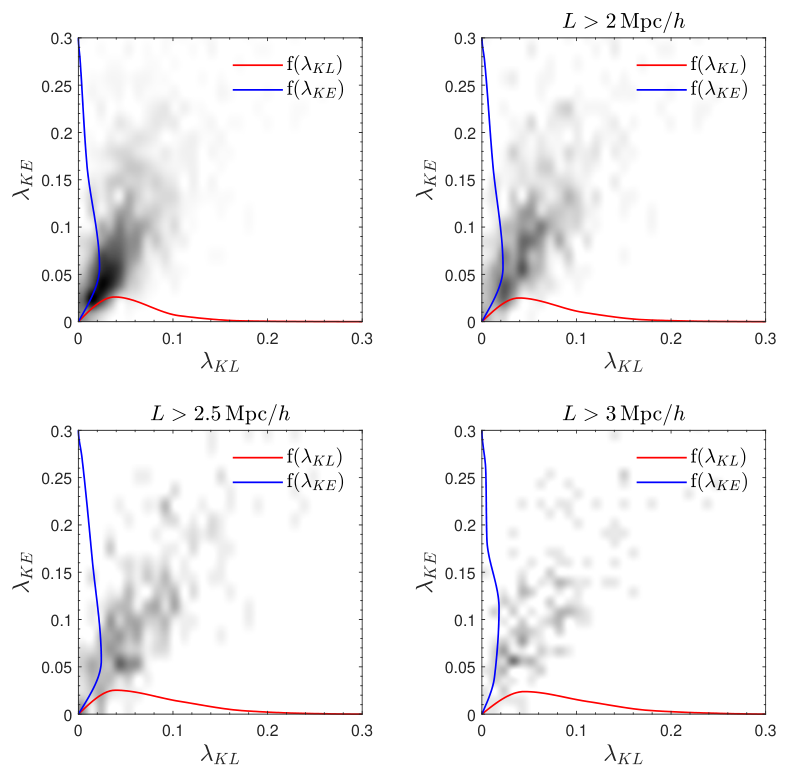
In Fig.4, we plot the correlation between $\lambda_{KL}$ and $\lambda_{KE}$ for filaments in different length ranges. Table 1 lists the number of filament samples and the correlation coefficient $r(\lambda_{KL},\lambda_{KL})$ as a function of filament spine length range. Figure 4 and Table 1 suggest that the spin magnitudes of $\boldsymbol{j}_{L}$ and $\boldsymbol{j}_{E}$ have a strong positive correlation. We find that this positive correlation is related to the length of the spine. Filaments with longer spines tend to have a stronger correlation between $\lambda_{KL}$ and $\lambda_{KE}$. This trend can be explained by the fact that longer filaments tend to be more filamentary in our samples as we have shown in the bottom left panel of Fig.2, which is partly a consequence of the limitation of the filament finder. By eliminating those filaments with low prolateness and ellipticity could make the correlation more robust.

By observing the PDFs of single parameters, we find that the values of $\lambda_{L}$ and $\lambda_{E}$ are much less than unity, suggesting that the filaments are not rotation supported in both Eulerian and Lagrangian spaces. This behavior is very similar to dark matter halos and protohalos by various of definitions (2021PhRvD.103f3522W).

To compare with the current observation works (2021NatAs.tmp..114W), which detected observational evidence for $\boldsymbol{j}^{\,\parallel}$, it is interesting to extract the spin magnitudes of $\boldsymbol{j}^{\,\parallel}$, which is parallel to the spine (${\mathbb{V}}_{1}$), and check whether it is correlated to their spin magnitudes in Lagrangian space. By projecting Eq.(4) onto a plane perpendicular to ${\mathbb{V}}_{1}$, the kinematic spin parameter becomes

where $x^{\prime\perp}=|\boldsymbol{x}^{\prime\perp}|$, $v^{\prime\perp}=|\boldsymbol{v}^{\prime\perp}|$, vectors with _⟂ are the components perpendicular to the spine. Here $\hat{\mathbb{V}}_{1}$ is an unit vector aligned with the spine. Because the spine is parity even, the sign of $\lambda_{E}^{\,\parallel}$ is defined according to the arbitrarily chosen $\hat{\mathbb{V}}_{1}$. Similarly, $\lambda_{L}^{\,\parallel}$ can be obtained from $\boldsymbol{j}_{L}^{\,\parallel}$ in the same manner,

With the above definition, $|\,\lambda_{L}^{\,\parallel}\,|,|\,\lambda_{E}^{\,\parallel}\,|\in[0,1]$, and larger $|\,\lambda_{L}^{\,\parallel}\,|$ or $|\,\lambda_{E}^{\,\parallel}\,|$ corresponds to more coherent rotations along the spine. Meanwhile, same/different signs of $\lambda_{L}^{\,\parallel}$ and $\lambda_{E}^{\,\parallel}$ indicates that $\boldsymbol{j}_{E}^{\,\parallel}$ is parallel/antiparallel to $\boldsymbol{j}_{L}^{\,\parallel}$.

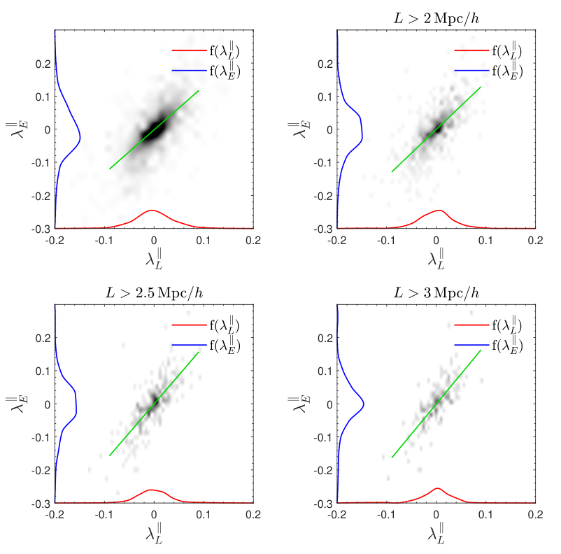
In Fig.5, we plot the correlation between $\lambda_{L}^{\,\parallel}$ and $\lambda_{E}^{\,\parallel}$ for filaments in different length ranges. The correlation coefficients $r(\lambda_{L}^{\,\parallel},\lambda_{E}^{\,\parallel})$ in different spine length range are also listed in Table 1. We find that the parallel component of the spin shows similar correlation as $\boldsymbol{j}$, the spin magnitudes of $\boldsymbol{j}_{L}^{\,\parallel}$ and $\boldsymbol{j}_{E}^{\,\parallel}$ have a strong positive correlation and filaments with longer spines tend to have a stronger correlation. Besides, the absolute values of $\lambda_{L}^{\,\parallel}$ and $\lambda_{E}^{\,\parallel}$ are also much less than unity, but fortunately the smallness of the rotation component of the filaments can still be measured (2021NatAs.tmp..114W).

In this subsection we reconstruct the predicted spins for filaments based on their Lagrangian space properties analogous to the the spin reconstruction of halos. As we have mentioned in Sec.III, the initial angular momentum vector of a protohalo that initially occupies Lagrangian volume $V_{L}$ is approximately by $\boldsymbol{j}\propto\epsilon_{ijk}I_{jl}T_{lk}$, where $\mathbf{I}=(I_{jl})$ is the moment of inertia tensor of $V_{L}$, $\mathbf{T}=(T_{lk})$ is the tidal tensor acting on $\mathbf{I}$, and $\epsilon_{ijk}$ is the Levi-Civita symbol collecting the antisymmetric components generated by the misalignment between $\mathbf{I}$ and $\mathbf{T}$. The spin reconstruction of dark matter halos is by defining (2020PhRvL.124j1302Y)

where $\boldsymbol{\mathcal{T}}$,$\boldsymbol{\mathcal{T}}^{+}$ are tidal fields constructed as Hessians of the initial gravitational potential smoothed at two different scales $r,R$. The initial gravitational potential can be estimated by the initial density field reconstructed method ELUCID, for which we refer the readers to (2014ApJ…794…94W; 2016ApJ…831..164W) for more details. This method can reproduce the density field of the nearby universe generated from the galaxy distributions in observation. To obtain $\boldsymbol{\mathcal{T}}$ and $\boldsymbol{\mathcal{T}}^{+}$, we smooth the initial gravitational potential $\phi_{\rm init}(\boldsymbol{q})$, by multiplying it in the Fourier space by the baryonic acoustic oscillation damping model ${\mathcal{D}}(k)^{1/4}=\exp{(-r^{2}k^{2}/2)^{1/4}}$ (2017PhRvD..95d3501Y). By choosing $R\to r_{+}$, we find $\boldsymbol{j}_{R}$ a good approximation for an angular momentum of a protohalo. Similarly, we apply this method to protofilaments, then we get the spin field $\boldsymbol{j}_{R}$ reconstructed from known initial conditions. We group all identified filaments into five mass bins, ranging from $\sim 10^{12}M_{\odot}$ to $\sim 10^{15.5}M_{\odot}$, then apply Eq.(8) with a set of different smoothing scales $r$, and compute the correlations between reconstructed and Eulerian spins of filaments. In Fig.6, we plot $\mu(\boldsymbol{j}_{E},\boldsymbol{j}_{R})$ as a function of smoothing scales $r$ and filament mass bins. The gray scale shows the degree of correlation and the darkest region in each mass bin represents the optimal smoothing scale $r_{\rm opt}$, also indicated by the yellow dashed curve.

We find that the spins of more massive filaments can generally be predicted at a wide range of smoothing scales. The correlation is larger than 0.3 for filaments more massive than $10^{13.5}M_{\odot}$. We also find that more massive filaments are better reconstructed by a larger smoothing radius, and this behavior is similar to the spin reconstruction of dark matter halos (2020PhRvL.124j1302Y). As a reference, we plot with the red dashed curve the equivalent protofilament radius in the Lagrangian space defined as $r_{q}\equiv(2MG/\Omega_{m}H^{2}_{0})^{1/3}$. We find that $r_{\rm opt}$ is not closely related to $r_{q}$, and find $\sim 5\,{\rm Mpc}/h$ a universal smoothing scale for all massive filaments.

References

- (1) P. J. E. Peebles, ApJ155, 393 (1969).
- (2) C. D. Rimes and A. J. S. Hamilton, MNRAS360, L82 (2005), astro-ph/0502081.
- (3) M. McQuinn, J. Cosmology Astropart. Phys2021, 024 (2021), 2008.12312.
- (4) H.-R. Yu, U.-L. Pen, and H.-M. Zhu, Phys. Rev. D95, 043501 (2017), 1610.07112.
- (5) Q. Pan, U.-L. Pen, D. Inman, and H.-R. Yu, MNRAS469, 1968 (2017), 1611.10013.
- (6) M. Iye, K.-i. Tadaki, and H. Fukumoto, ApJ886, 133 (2019), 1910.10926.
- (7) A. G. Doroshkevich, Astrofizika 6, 581 (1970).
- (8) S. D. M. White, ApJ286, 38 (1984).
- (9) C. Porciani, A. Dekel, and Y. Hoffman, MNRAS332, 325 (2002), astro-ph/0105123.
- (10) H.-R. Yu, U.-L. Pen, and X. Wang, Phys. Rev. D99, 123532 (2019), 1810.11784.
- (11) A. F. Teklu et al., ApJ812, 29 (2015), 1503.03501.
- (12) J. Lee and U.-L. Pen, ApJ532, L5 (2000), astro-ph/9911328.
- (13) J. Lee and U.-L. Pen, ApJ555, 106 (2001), astro-ph/0008135.
- (14) H.-R. Yu et al., Phys. Rev. Lett.124, 101302 (2020), 1904.01029.
- (15) H. Wang, H. J. Mo, X. Yang, Y. P. Jing, and W. P. Lin, ApJ794, 94 (2014), 1407.3451.
- (16) P. Motloch, H.-R. Yu, U.-L. Pen, and Y. Xie, Nature Astronomy 5, 283 (2021), 2003.04800.
- (17) I. B. Zeldovich, J. Einasto, and S. F. Shandarin, Nature300, 407 (1982).
- (18) J. R. Bond, L. Kofman, and D. Pogosyan, Nature380, 603 (1996), astro-ph/9512141.
- (19) M. C. Neyrinck, MNRAS460, 816 (2016), 1510.03431.
- (20) M. Neyrinck, M. A. Aragon-Calvo, B. Falck, A. S. Szalay, and J. Wang, The Open Journal of Astrophysics 3, 3 (2020), 1904.03201.
- (21) Q. Xia, M. C. Neyrinck, Y.-C. Cai, and M. A. Aragón-Calvo, MNRAS506, 1059 (2021), 2006.02418.
- (22) P. Wang, N. I. Libeskind, E. Tempel, X. Kang, and Q. Guo, Nature Astronomy (2021), 2106.05989.
- (23) H.-R. Yu, U.-L. Pen, and X. Wang, ApJS237, 24 (2018), 1712.06121.
- (24) Y. B. Zel’dovich, A&A5, 84 (1970).
- (25) T. Sousbie, MNRAS414, 350 (2011), 1009.4015.
- (26) T. Sousbie, C. Pichon, and H. Kawahara, MNRAS414, 384 (2011), 1009.4014.
- (27) D. Novikov, S. Colombi, and O. Doré, MNRAS366, 1201 (2006), astro-ph/0307003.
- (28) T. Bonnaire, N. Aghanim, A. Decelle, and M. Douspis, A&A637, A18 (2020), 1912.00732.
- (29) L. A. Pereyra, M. A. Sgró, M. E. Merchán, F. A. Stasyszyn, and D. J. Paz, MNRAS499, 4876 (2020), 1911.06768.
- (30) E. Tempel et al., MNRAS438, 3465 (2014), 1308.2533.
- (31) R. S. Stoica, V. J. Martínez, and E. Saar, Journal of the Royal Statistical Society: Series C (Applied Statistics) 56, 459 (2007).
- (32) R. S. Stoica, V. J. Martínez, and E. Saar, A&A510, A38 (2010), 0912.2021.
- (33) J. Hui, M. Aragon, X. Cui, and J. M. Flegal, MNRAS475, 4494 (2018), 1803.11156.
- (34) O. Hahn, C. Porciani, C. M. Carollo, and A. Dekel, MNRAS375, 489 (2007), astro-ph/0610280.
- (35) N. A. Bond, M. A. Strauss, and R. Cen, MNRAS409, 156 (2010), 1003.3237.
- (36) J. E. Forero-Romero, Y. Hoffman, S. Gottlöber, A. Klypin, and G. Yepes, MNRAS396, 1815 (2009), 0809.4135.
- (37) M. A. Aragón-Calvo, B. J. T. Jones, R. van de Weygaert, and J. M. van der Hulst, A&A474, 315 (2007), 0705.2072.
- (38) M. Cautun, R. van de Weygaert, and B. J. T. Jones, MNRAS429, 1286 (2013), 1209.2043.
- (39) M. Cautun, R. van de Weygaert, B. J. T. Jones, and C. S. Frenk, MNRAS441, 2923 (2014), 1401.7866.
- (40) C. Porciani, A. Dekel, and Y. Hoffman, MNRAS332, 339 (2002), astro-ph/0105165.
- (41) Q. Wu, H.-R. Yu, S. Liao, and M. Du, Phys. Rev. D103, 063522 (2021), 2011.03893.
- (42) H. Wang et al., ApJ831, 164 (2016), 1608.01763.
- (43) E. J. Baxter, B. D. Sherwin, and S. Raghunathan, J. Cosmology Astropart. Phys2019, 001 (2019), 1904.04199.