DOCKSTRING: easy molecular docking yields better benchmarks for ligand design
Abstract
The field of machine learning for drug discovery is witnessing an explosion of novel methods. These methods are often benchmarked on simple physicochemical properties such as solubility or general druglikeness, which can be readily computed. However, these properties are poor representatives of objective functions in drug design, mainly because they do not depend on the candidate’s interaction with the target. By contrast, molecular docking is a widely successful method in drug discovery to estimate binding affinities. However, docking simulations require a significant amount of domain knowledge to set up correctly which hampers adoption. To this end, we present dockstring, a bundle for meaningful and robust comparison of ML models consisting of three components: (1) an open-source Python package for straightforward computation of docking scores; (2) an extensive dataset of docking scores and poses of more than 260K ligands for 58 medically-relevant targets; and (3) a set of pharmaceutically-relevant benchmark tasks including regression, virtual screening, and de novo design. The Python package implements a robust ligand and target preparation protocol that allows non-experts to obtain meaningful docking scores. Our dataset is the first to include docking poses, as well as the first of its size that is a full matrix, thus facilitating experiments in multiobjective optimization and transfer learning. Overall, our results indicate that docking scores are a more appropriate evaluation objective than simple physicochemical properties, yielding more realistic benchmark tasks and molecular candidates.
1 Introduction
The field of industrial drug discovery is undergoing a crisis. Despite significant technological advances, R&D costs have grown by orders of magnitude while the probability of success of candidate molecules has decreased. This phenomenon is partly attributed to a lack of sufficiently predictive experimental and computational models Scannell and Bosley 2016. Machine learning (ML) is widely regarded as a promising technology to tackle this issue by providing faster and more accurate models Bender and Cortés-Ciriano 2021.
The rapid development of ML methods for drug discoveryVamathevan et al. 2019; Lavecchia 2015 has resulted in a growing need for high-quality benchmarks to allow for these methods to be evaluated and compared. Ideally, a good benchmark would test a model on accurate experimental data (e.g. experimental bioactivity data) in a realistic problem setting (e.g. prospective search), so that strong performance on the benchmark would imply strong performance on real-world tasks. Unfortunately, the high cost and difficulty of collecting experimental data makes such benchmarks impractical. Existing benchmarks tend to either (1) use a fixed experimental dataset for problem settings like in-distribution regressionWu et al. 2018, or (2) use simple computational properties for problem settings like de novo design. The latter type of benchmark is popular in the ML community with the tasks of maximizing the quantitative estimate of druglikeness (QED) Bickerton et al. 2012 and penalized log partition coefficient (logP) being highly prevalent.Xu et al. 2020; Ahn et al. 2020; Mollaysa et al. 2020; Samanta et al. 2020; Maziarka et al. 2020; Thiede et al. 2020; Wu et al. 2020; Tripp et al. 2020 However, the simplicity of these properties raises doubts about whether performance on such benchmarks is indicative of performance on real drug-design tasks.
Previous works have suggested that molecular docking could form the basis for high-quality benchmarks.Coley et al. 2020; Cieplinski et al. 2021; Huang et al. 2021 Molecular docking is a computational technique that predicts how a small molecule (the ligand) binds to a protein receptor (the target) by simulating the physical interaction between the two.Varela-Rial et al. 2021 The output of this simulation is a docking score, which represents the strength of binding between the molecule and protein, and a docking pose, the predicted 3D conformation of the ligand in the protein binding pocket. Below, we summarize some of the benefits of molecular docking over simple physicochemical properties (e.g., logP):
- 1.
Interpretability: docking scores have a clear biological interpretation in terms of binding affinity Kitchen et al. 2004, correlating with experimental values in some protein familiesSu et al. 2019.
- 2.
Relevance: docking scores are routinely employed by medicinal chemists in academia and industry to discover hits in virtual screening experiments. Docking poses are also used to identify and exploit important interactions during lead optimization.
- 3.
Computational cost: docking scores can typically be computed in under a minute, unlike other computational methods like free energy perturbation calculations or density-functional theory.
- 4.
Challenging benchmark: the relationship between molecular structure and docking score is complex, as the docking score depends on the 3D structure of the ligand-target complex. Therefore, tasks based on docking require ML models to learn complex 3D features.
Because of these advantages it is unsurprising that several recent works have applied ML to tasks based on docking scores.Jeon and Kim 2020; Graff et al. 2021; Thomas et al. 2021; Gentile et al. 2020; Lyu et al. 2019. Yet, there are still several hurdles which make a docking benchmark difficult to realize. First, such a benchmark mandates high-quality standardization. Running a docking simulation involves many intermediate steps, such as target and ligand preparation and the specification of a search box. Each step requires significant domain expertise, and for a benchmark to facilitate a meaningful comparison between algorithms, they must be carried out correctly and consistently. Second, the benchmark needs to be accessible to those without domain knowledge. Finally, the benchmark needs to contain breadth and diversity of targets.
A fully-automated docking software pipeline is a potential way to overcome these hurdles. Indeed, there are several existing works which try to facilitate the use of molecular docking for ML benchmarks. However, these works all lack at least one of the aforementioned desiderata. VirtualFlow Gorgulla et al. 2020 and DockStream Guo et al. 2021 (part of the REINVENT ecosystemBlaschke et al. 2020) are general-purpose wrappers for docking programs. However, they primarily cater docking experts requiring manually-prepared target files and specialized arguments. The Therapeutics Data Commons (TDC) Huang et al. 2021 and Cieplinski et al.Cieplinski et al. 2021 provide wrappers which offer computation of docking scores from just a SMILES string. However, both wrappers have shortcomings with respect to standardization. Neither TDC nor Cieplinski et al. control sources of randomness during the docking procedure (e.g., random seeds input into the docking program or the conformer generation routines) leading to the potential for considerable variance between runs on the same molecule. Further, at the time of writing, both wrappers have a relatively rudimentary ligand preparation pipeline: for example, neither of them perform ligand protonation, an important part of the preparation process Brink and Exner 2009; Bender et al. 2021. Moreover, both of these wrappers provide only a small number of targets: TDC provides only one target, while Cieplinski et al.Cieplinski et al. 2021 provide just four.
In addition to wrappers, several docking benchmarks have been developed. The Directory of Useful Decoys Enhanced (DUD-E) Mysinger et al. 2012 is a relatively small ligand set of actives and property-matched decoys for 102 targets. Originally designed to evaluate docking algorithms, its ligand set has since been widely applied to benchmark ML models for virtual screening Wallach et al. 2015; Yan et al. 2017; Ragoza et al. 2017. However, it has been argued that simple physicochemical properties (e.g., molecular weight or logP) are not sufficient to match actives and decoys against ML algorithms, so these can simply memorize the actives and inactives, overfitting and complicating generalization. Therefore, ML methods employing the ligand set in DUD-E are likely to overestimate virtual screening performance Chen et al. 2019; Sieg et al. 2019. The evaluation framework GuacaMol Brown et al. 2019 provides both a distribution matching and goal-directed benchmark suite, with the latter containing 20 distinct tasks based on molecular fingerprints, substructure matching, and physicochemical properties. Although most of these tasks are challenging, they are largely based on simple physicochemical properties and similarity functions such as the Tanimoto similarity. As a result, they fail to capture subtleties related to 3D molecular structure or interactions with biomolecules. The benchmark suite MOSES Polykovskiy et al. 2020 provides several molecular generation benchmarks that focus on generating a diverse set of molecules rather than optimizing for any particular chemical property.
In this work, we introduce dockstring, a bundle for standardized and accessible benchmarking of ML models based on molecular docking. It consists of three parts: a Python package for easy computation of docking scores; a large and diverse dataset of docking scores and poses for pre-training; and a set of meaningful benchmark tasks on which to evaluate models.
- 1.
Python package: a user-friendly Python wrapper of the popular docking package AutoDock Vina Trott and Olson 2010 (Sections 2.1 and 3.1). AutoDock Vina was selected due to its high-quality docking poses, reasonable accuracy of predicted binding free energies, and low computational cost Su et al. 2019; Pagadala et al. 2017. The emphasis of our package is on simplicity—a docking simulation can be setup in just four lines of code.
- 2.
Dataset: a dataset of over 260K diverse and druglike molecules docked against a curated list of 58 targets, resulting in more than 15M docking scores and poses (Sections 2.2 and 3.2). The high number of activity labels per ligand makes our dataset highly suitable for the design of meaningful benchmark tasks in ML settings such as multi-objective optimization or transfer learning. Furthermore, targets are selected to represent a number of protein families of high pharmaceutical value, such as kinases or nuclear receptors. Overall, more than 500K CPU hours were invested in the creation of the dataset.
- 3.

2 Methods
2.1 Python Package
2.1.1 Target Preparation
There are 58 prepared targets available in dockstring. PDB files of 57 protein targets were downloaded from the Directory of Useful Decoys Extended (DUD-E), a database of proteins and ligands for benchmarking docking algorithms Mysinger et al. 2012. Structures in DUD-E were determined experimentally to high precision, with the large majority of resolutions being less than 2.5 Å. Furthermore, DUD-E targets were prepared to improve correlation between theoretical and experimental binding affinities. For instance, in a few cases, the authors of DUD-E manually added cofactors or crystallographic waters, or changed the protonation states of side residues Mysinger et al. 2012. For dockstring, the PDB files were standardized with Open Babel O’Boyle et al. 2011 (e.g., the symbols of some metal atoms were not recognized by AutoDock Tools Morris et al. 2009), polar hydrogen atoms were added, and conversion to the PDBQT file format was carried out with AutoDock Tools.
The only target that does not originate from DUD-E is DRD2, the dopamine receptor D2.
It was included in dockstring due to its popularity in molecular regression and optimization Olivecrona et al. 2017; Arús-Pous
et al. 2020; Maragakis et al. 2020; Jin et al. 2018; Jin et al. 2019.
To ensure consistency, the preparation of DRD2 was analogous to that of its homolog DRD3 in DUD-E.
Starting from a crystal structure of DRD2 (PDB entry 6CM4) Wang et al. 2018,
the bound inhibitor (risperidone) as well as residual water and solute molecules were manually removed with PyMOL DeLano 2015, since DRD3 in DUD-E did not include any waters or ions.
Subsequently, the structure was optimized with the program obminimize from Open Babel using the general Amber force field (GAFF) Wang et al. 2004.
Protonation was carried out at pH 7.4 with PROPKA Olsson et al. 2011.
Finally, addition of polar hydrogen atoms and conversion to PDBQT was performed with AutoDock Tools.
The search box of each target in dockstring was also determined. Every DUD-E structure has a corresponding ligand file from which the box position and size were derived. We computed the maximum and minimum coordinates of each ligand across each dimension and padded with 12.5 Å on all sides. Finally, if a box length did not reach 30 Å after padding, we set it to this amount. The padding length and the minimum box length were tuned manually to minimize the number of positive scores, which indicate highly constrained poses. The search box of DRD2 was set manually upon visual examination of the binding pocket in the reference structure bound to risperidone Wang et al. 2018.
2.1.2 Ligand Preparation
Ligands are provided to the dockstring package as SMILES strings. First, dockstring performs a sanity check on the ligand. Ligands with radicals or ligands consisting of more than one molecular fragment are rejected. Next, the ligand is (de-)protonated at pH 7.4 with Open Babel O’Boyle et al. 2011. While automated protonation protocols are not perfect Brink and Exner 2009, their application is widely regarded as good practice Bender et al. 2021. Then, a single three-dimensional (3D) conformation is generated with the Euclidean distance geometry algorithm ETKG Riniker and Landrum 2015 as implemented in RDKit Landrum 2021. This conformation is subsequently refined with the classical force field MMFF94 Halgren 1996. During the embedding of the graph representation into a 3D structure, the stereochemistry of determined stereocenters is maintained, whereas any undetermined stereocenters are assigned randomly (but consistently across different runs to ensure the reproducibility of docking scores). Finally, dockstring computes the Gasteiger charges Gasteiger and Marsili 1980 for all atoms and creates a ligand PDBQT file with Open Babel.
2.1.3 Molecular Docking with AutoDock Vina
dockstring docks a ligand against a target using AutoDock Vina Trott and Olson 2010. The ligand PDBQT input file is obtained automatically as explained in Section 2.1.2, while the target PDBQT and search boxes are taken from the list of prepared input files as explained in Section 2.1.1. Docking is performed with the default values of exhaustiveness (8), maximum number of binding modes (9) and energy range (3). After docking is complete, we obtain up to nine poses, together with their binding free energies. Note that in subsequent analyses, we only use the lowest docking score (i.e. the best one).
Ligand preparation and molecular docking, and thus the docking score, depend on a random seed. We investigated this dependence and found no target-ligand combination for which the docking scores deviated by more than kcal/mol. Subsequently, we fixed the random seed to obtain a fully deterministic pipeline.
2.2 Dataset
2.2.1 Target and ligand selection
As explained in Section 2.1.1, most targets originate from from DUD-E Mysinger et al. 2012, a database of proteins and ligands for comparison and development of docking algorithms. These targets are medically relevant and cover a large variety of protein families, functions, and structures. We only selected targets with more than 1000 experimental actives in ExCAPE Sun et al. 2017, a database that curates bioactivity assays from PubChem Kim et al. 2021 and ChEMBL Mendez et al. 2019, to ensure a high number of positive examples. In addition to the targets from DUD-E, we also included the target DRD2, a popular benchmark in ML Olivecrona et al. 2017; Arús-Pous et al. 2020; Maragakis et al. 2020; Jin et al. 2018; Jin et al. 2019.
The ligands and their experimental activity labels originate from ExCAPE Sun et al. 2017. We selected all ligands with active labels against the proteins in our target set (at least 1000 actives for each target). We believe that the large number of positive examples will create a strong signal that will facilitate learning in tasks that require experimental labels. We also added 150K ligands which only had inactive labels against our targets. After discarding 1.8% of molecules due to failures in the ligand preparation process, the final dataset consisted of compounds.
2.2.2 Clustering and scaffold analysis
Density-Based Spatial Clustering of Applications with Noise (DBSCAN) was implemented with scikit-learn Pedregosa et al. 2011. Prior to executing DBSCAN, molecules were embedded in a space of RDKit fingerprints of path length six and set the neighborhood cutoff to a Jaccard distance of 0.25 Bender and Glen 2004. The choice of the fingerprints was motivated by previous analysis by Landrum Landrum 2021 suggesting that this type of fingerprint was the most appropriate for similarity search. Bemis-Murcko scaffold decomposition was implemented with RDKit.
2.3 Benchmarks
dockstring’s combination of a docking package and large dataset allows it to underpin a wide variety of benchmark tasks for supervised learning, active learning, transfer learning, meta-learning, molecule optimization and more. We formulate benchmark tasks for three problem settings: regression, virtual screening, and de novo design (Table 1). The regression benchmark (Sections 2.3.1 and 3.3.1) is relatively standard and widely applicable; it primarily illustrates the difficulty of predicting docking scores. Virtual screening (Sections 2.3.2 and 3.3.2) evaluates a model’s ability to select active molecules from a large predefined library. This is a common use case for predictive models in the pharmaceutical industry and requires strong out-of-distribution performance to be successful. It is applicable to any method that can rank a list of molecules, either by regression or by other means. De novo design (Sections 2.3.3 and 3.3.3) evaluates the ability to generate novel molecules that optimize an objective function. It is an active area of research because chemical space is vast (more than by some estimates Bohacek et al. 1996), so even the largest libraries cover just a tiny fraction of it. Models for de novo design include optimization algorithms, reinforcement learning agents, or generative models. The objective functions presented here are all based on docking scores but vary in difficulty.
| Setting | Description | Motivation | Proteins | Metric |
| Regression | Predict docking scores and minimize prediction error on held-out test set | Evaluation of molecular representations and predictive models | PARP1, F2, KIT, ESR2, PGR | Coefficient of determination () |
| Virtual screening | Rank molecules according to their docking score and compute enrichment in top--ranking molecules | Model evaluation for hit discovery in large molecular libraries | PARP1, KIT, PGR | Enrichment factor (EF) |
| De novo design | Given a training dataset and a fixed budget of objective function evaluations, propose molecules that optimize an objective | Model evaluation for hit discovery by de novo molecular design | F2 PPAR{A, D, G} JAK2, LCK |
2.3.1 Regression
Task description. For each target, the task is to train a regression model to predict the docking score of a given SMILES string. The models were trained and tested on the dockstring dataset, split into training and test sets according to the cluster labels (see Section 3.2.2). Cluster splitting is recommended because chemical datasets contain many analogous (yet unique) molecules, such that simple random split will likely lead to an overestimation of test performance.
Proposed benchmark. While all targets could be used in this benchmark, the large number of targets in our dataset would make this benchmark expensive and difficult to interpret. Therefore, we selected five targets from different protein families whose docking scores were deemed of high quality, based on enrichment analysis of experimental activity labels (Section 3.2.1). To ensure that we included a range of difficulties, we performed an initial experiment where we regressed the docking scores of all high-quality targets. We found that performance varied considerably depending on the target and the method employed, with coefficients of determination ranging between and (details in Table 3 of the Supporting Information (SI)). Based on these results, we proposed the five following benchmark targets (with protein function and level of difficulty in brakets): PARP1 (enzyme, easy), F2 (protease, easy to medium), KIT (kinase, medium), ESR2 (nuclear receptor, hard), and PGR (nuclear receptor, hard).
2.3.2 Virtual Screening
Task description. The goal of screening is to identify actives from a large library that is too big for detailed experimental analysis. Screening methods attempt to solve this issue by first scoring the library and selecting a smaller subset enriched with high scores (in virtual screening, the scoring is done computationally). Then, the subset can be studied in more detail. A metric that is typical of screening experiments is the enrichment factor (EF), defined as the rate of actives in the selected subset over the rate of actives in the initial library. Here, we propose to rank all (around 1 billion) compounds in the ZINC20 database of commercially available druglike molecules Irwin et al. 2012; Irwin et al. 2020 and compute the enrichment factor (EF) of the top-ranking subset. Since ground-truth labels are not available for all molecules in ZINC20, we mark a molecule as active if its docking score is lower (i.e., better) than a certain threshold. We chose this threshold to be the lowest percentile in the ZINC20 database, which we estimated from a random sample of 100K molecules. Therefore, the maximum possible enrichment in our experiments is 1000.
Proposed benchmark. We trained models on the docking scores of PARP1, KIT, and PGR using all molecules in our dataset. As in the regression benchmark, these targets were chosen to represent a range of regression difficulties. Trained models were used to rank all the molecules in ZINC20 and select the top 5000 compounds with the lowest predicted scores. Once the most promising molecules had been selected, we computed their actual docking scores with dockstring. Molecules were labelled as active if their actual scores were below the 0.1 percentile threshold which was -10.7 for KIT, -12.1 for PARP1, and -10.1 for PGR. Finally, the enrichment factor (EF) was computed as the ratio of active molecules in the selected subset over the ratio of active molecules in ZINC20. Note that the latter is 0.1% by design.
Note that the virtual screening benchmark is distinct from the regression benchmark in that it only requires ranking compounds instead of explicitly predicting docking scores. Further, it uses a different evaluation metric, the EF, which is uncommon in the ML literature but popular in cheminformatics. This metric evaluates only the top molecules, whereas regression metrics depend on the predictions of all molecules.
2.3.3 De novo Molecular Design
Task description. The goal of de novo design is to propose novel molecules that optimize an objective function given a certain budget. To be representative of real problems in drug discovery, this budget should be high enough to allow for significant exploration but small enough to resemble the experimental budget of a committed wet lab.
Docking scores are biased towards high molecular weight and lipophilicity. Therefore, optimizing docking scores alone can lead to large and hydrophobic molecules, as we observed in our initial experiments (Figure 9). These compounds are undesirable because they will suffer from poor ADMET properties and off-target effectsCarta et al. 2007; Hopkins et al. 2014. We found that adding a druglikeness penalty based on QED helped remedy this issue.
Proposed benchmark. The goal of each de novo design task is to minimize a docking-based objective function, having access to the whole dataset and 5000 function evaluations. In the case of predictive generative models such as GP-BO, the whole dataset could be used to learn the docking score function, whereas in genetic algorithms it could be used to set the initial population. We propose three objective functions, all of which contain a weighted QED term to promote druglikeness. Let be a target, be a ligand, and be the docking score of against . Let be the QED value of .
- 1.
F2: a comparatively easy task that requires docking well to a single protein.
(1) - 2.
Promiscuous PPAR: requires strong binding to the three PPAR nuclear receptors. PPAR scores are positively correlated, so this is a task of medium difficulty. “Promiscuous” pan-PPAR agonists are being researched as treatments against metabolic syndrome Staels and Fruchart 2005. If , then the objective function is
(2) - 3.
Selective JAK2: requires strong binding to JAK2 and weak binding to LCK. The challenge is that, since they are both kinases, their scores are positively correlated (). Due to their role in cell signaling and cancer, kinases are highly relevant targets but achieving selectivity is notoriously difficult, and off-target effects and toxicity are common Ferguson and Gray 2018. Our proposed objective anchors the LCK score to its median ():
(3)
2.4 Baselines
We tested a variety of classical and more modern algorithms to assess the difficulty of the dockstring benchmarks tasks. Training and testing datasets and procedures followed each tasks’ specifications as described in Section 2.3. Additional details are given in the SI.
2.4.1 Regression and virtual screening
scikit-learn algorithms.
Ridge and lasso regression were implemented with scikit-learn. XGBoost was implemented with the XGBoost library Chen and Guestrin 2016 using the scikit-learn API. For all these methods, hyperparameter selection was done with random search over 20 configurations, evaluating each configuration using a 5-fold cross-validation score (implemented via scikit-learn’s RandomizedSearchCV function).
Gaussian processes.
All Gaussian process (GP) algorithms used the Tanimoto kernel Tanimoto 1958 with fingerprint features. Due to the cubic scaling of GP regression, the exact GP was trained on 10K randomly chosen data points. In comparison, the sparse GP used 10K randomly chosen training points as the inducing variables, but was trained on the whole dataset. Hyperparameters were chosen by maximizing the log-marginal likelihood on the training set. All GPs were implemented with PyTorch Paszke et al. 2019 and GPyTorch Gardner et al. 2018.
Graph neural networks.
The DeepChem library’s implementation of the Attentive FP and MPNN was used Ramsundar et al. 2019. Both models were trained with default parameters from the DeepChem library for 10 epochs. Preliminary experiments with a third method from DeepChem, the Graph Attention Network Veličković et al. 2018, were performed but the model frequently overfitted to the training data; we decided to omit it rather than tune the hyperparameters for this model.
2.4.2 De novo design
Graph genetic algorithm.
The implementation from the GuacaMol baselines Brown et al. 2019 was usedgua. The population size was set to 250, the offspring size to 25, and the mutation rate to 0.01. The population size was chosen based on some preliminary experiments with the GuacaMol dataset, and the offspring size was arbitrarily chosen to be 25 to allow for 200 generations to occur. The value of the mutation rate was the default used in the GuacaMol implementation.
SELFIES genetic algorithm.
The implementation of the SELFIES genetic algorithm was taken from the GitHub repository of Nigam et al Nigam et al. 2021. It is a simple genetic algorithm which randomly inserts, deletes, or modifies a single token of a SELFIES string Krenn et al. 2020. The algorithm was not tuned and represents the minimum level of performance that can be expected from any reasonable genetic algorithm. The offspring and population size hyperparameters were the same as for the graph genetic algorithm.
Bayesian optimization.
The GP implementation is identical to the exact GP implementation from Section 3.3.1 using the Tanimoto kernel Tanimoto 1958; Ralaivola et al. 2005. As it is computationally infeasible to train a GP on the entire dataset, the 2000 training points with the smallest objective score and 3000 random points were selected from the dataset for training. Kernel hyperparameters were chosen by maximizing the log marginal likelihood on this training set. At each iteration, a batch of five new molecules was selected by maximizing either the upper confidence bound acquisition function Srinivas et al. 2010 with (i.e., ) or the expected improvement acquisition function Jones et al. 1998. was chosen based on the GP hyperparameters from Section 3.3.1 and a small amount of preliminary experiments on the GuacaMol benchmarks to encourage a combination of exploration and exploitation, but was not tuned once experiments on the docking objectives were started. Optimization was done using the graph genetic algorithm as described above, with an offspring size of 1000 and 25 generations. The batch was then scored and the GP retrained using the new scores, with the hyperparameters remaining unchanged. This was repeated until the objective function evaluation budget was reached.
3 Results
This section introduces the three components of the dockstring bundle: a user-friendly molecular docking package, an extensive dataset, and a set of challenging benchmark tasks. The package is available at https://github.com/dockstring/dockstring, while the dataset and code for benchmark baselines are available at https://figshare.com/s/95f2fed733dec170b998. All components are released under the Apache 2.0 license.
3.1 Molecular Docking Package
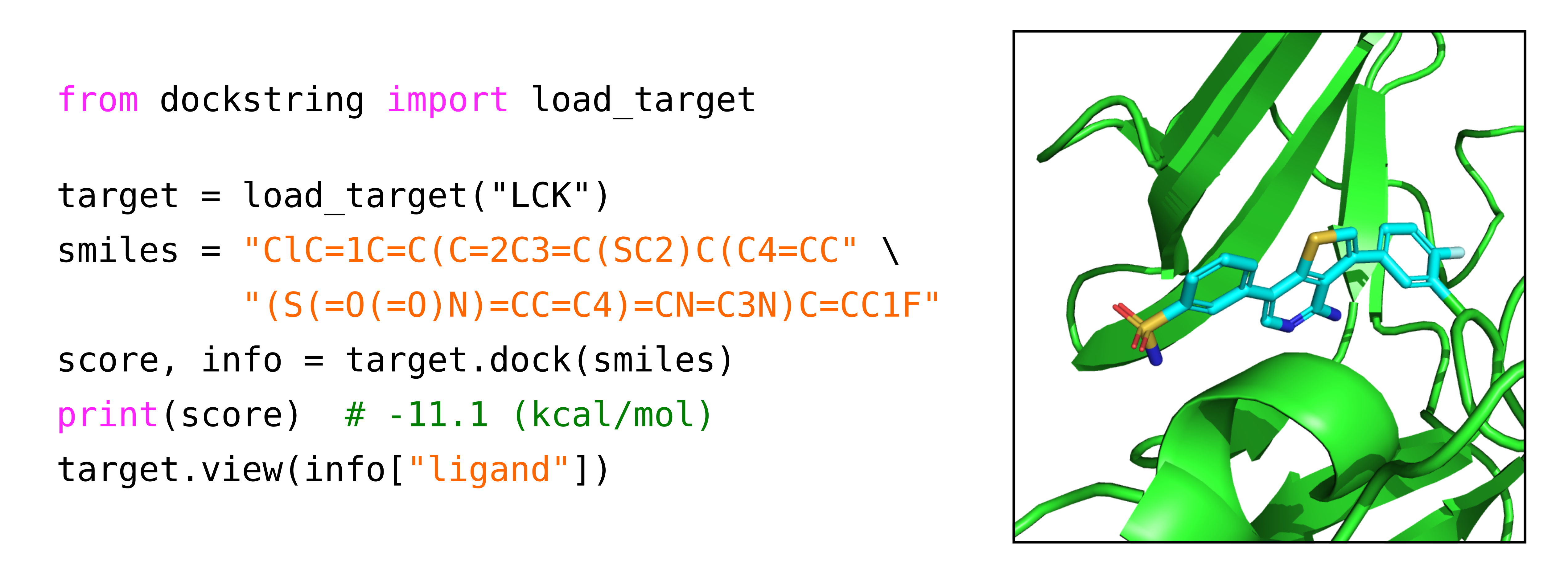
We developed a Python package that interfaces with AutoDock Vina to allow the computation of docking scores in just a few lines of code. The user only needs to provide the name of a target protein and the SMILES string of a ligand molecule (Figure 2, left). The target name can be chosen from a list of 58 targets (Table 2) that have been prepared as explained in Section 2.1.1. Ligands are prepared automatically by the dockstring package as explained in Section 2.1.2. dockstring returns up to nine docking poses with their corresponding docking scores, which can be used in downstream tasks such as bioactivity prediction and visualization (Figure 2, right). Note that in subsequent experiments in this work, we always use the lowest (i.e. best) docking score. For most targets, computing a score with eight CPUs takes around 15s (Table 5 of the SI). We also note that, by default, our docking wrapper carefully controls all sources of randomness in the docking procedure so that the output is deterministic (see Section 2.1.3). Finally, the target, the search box, and all poses can be visualized with the PyMOL software package.
3.2 Dataset
Molecular docking is applicable in areas such as regression, molecular optimization, virtual screening, transfer learning, multi-task learning, and representation learning. Since most of these settings require an initial training dataset, we provide a set of more than 15 million scores for a diverse and highly-curated set of more than ligands docked against 58 targets. This dataset required more than 500K CPU hours to compute (see Section D of the SI for computational details). The target and ligand selection process are detailed below.
3.2.1 Target Selection
Our dataset comprises 58 targets covering a variety of protein functions: kinases (22), enzymes (12), nuclear receptors (9), proteases (7), G-protein coupled receptors (5), cytochromes (2), and chaperone (1). For details, see Table 2. We have identified a subset of 24 targets whose docking scores are of relatively high quality based on their ability to achieve enrichment of experimental active labels (details are given in Section 3.2.3). These high-quality targets are involved in a range of diseases and are thus considered of great interest in drug discovery (examples can be seen in Table 2 of the SI).
| Group | Quality | Gene |
| Kinase | *** | IGF1R, JAK2, KIT, LCK, MAPK14, MAPKAPK2, MET, PTK2, PTPN1, SRC |
| ** | ABL1, AKT1, AKT2, CDK2, CSF1R, EGFR, KDR, MAPK1, FGFR1, ROCK1 | |
| * | MAP2K1, PLK1 | |
| Enzyme | *** | HSD11B1, PARP1, PDE5A, PTGS2 |
| ** | ACHE, MAOB | |
| * | CA2, GBA, HMGCR, NOS1, REN, DHFR | |
| Nuclear Receptor | *** | ESR1, ESR2, NR3C1, PGR, PPARA, PPARD, PPARG |
| ** | AR | |
| * | THRB | |
| Protease | *** | ADAM17, F10, F2 |
| ** | BACE1, CASP3, MMP13 | |
| * | DPP4 | |
| GPCR | ** | ADRB1, ADRB2, DRD2, DRD3 |
| * | ADORA2A | |
| Cytochrome | ** | CYP2C9, CYP3A4 |
| Chaperone | * | HSP90AA1 |
3.2.2 Ligand Selection and Clustering
ExCAPE is a large database that aggregates results from a variety of assays in PubChem and ChEMBL, many of them from real screening experiments for hit discovery. Furthermore, it sets explicit filters for physicochemical properties such as molecular weight and number of heavy atoms to further promote druglikeness. For these reasons, ExCAPE is generally regarded as diverse and druglike. Indeed, we found that most ligands fulfill Lipinski’s rules Lipinski et al. 2001 and feature favorable QED profiles (Figure 3).
We performed cluster analyses with two different techniques: DBSCAN (Density-Based Spatial Clustering of Applications with Noise), a data-type agnostic clustering algorithm, and Bemis-Murcko scaffold decomposition, which is especially designed for molecules. Given a cluster and a query point, DBSCAN assigns a point to the cluster if it is within the -neighborhood of one of its core points (where a core point is one that has a minimum number of neighbors from the same cluster)Ester et al. 1996. DBSCAN found 52K clusters, where the biggest one covered over 15% of the dataset and 31K clusters contained only a single molecule (Figure 4, left). The Jaccard distance within the same cluster was significantly smaller than the distance between different clusters, with little overlap of the two (Figure 4, middle).
Bemis-Murcko decomposition is rooted in the concept of molecular scaffolds Bemis and Murcko 1996. A scaffold is defined as the union of the ring systems in a molecule plus the linker atoms between them. Thus, there are many possible molecules with the same scaffold that differ only in their side chains and atom types. Molecules with the same scaffold are structurally similar and are expected to have similar properties. We found that our ligand set contains 102K Bemis-Murcko scaffolds. They showed a similar distribution to DBSCAN clusters, with the most popular scaffold standing out from the rest and 64K single-molecule scaffold clusters (Figure 4, right). Overall, these results confirm that our ligand set is diverse.
3.2.3 Docking Scores
We computed docking scores for every target-ligand pair in our dataset, resulting in more than 15M data points (see Section D of the SI for computational details). To our knowledge, this is the first dataset that computes the full score matrix of a large ligand set against a high number of protein targets, making it ideal for the design of meaningful benchmark tasks in settings such as multiobjective optimization and transfer learning.
We found that the docking scores were similarly distributed for most proteins, ranging between and , as can be seen in Figure 5 (note that in the original AutoDock Vina publicationTrott and Olson 2010 scores are reported in kcal/mol, but for our purposes scores can be treated as a unitless quantity). Docking scores can be interpreted as the binding free energy, so more negative scores suggest stronger binding. We also found that high-quality targets that were functionally related or were homologs (i.e., proteins with high sequence similarity such as ESR1 and ESR2) exhibited high correlation, whereas unrelated targets tended to show medium or poor correlation (Figure 6). This supports the claim that dockstring scores are biologically meaningful.

We assessed the quality of each target’s docking scores based on their enrichment factor (EF), using experimental activity labels from ExCAPE as reference (Figure 7). Such assessment was necessary because docking is known to perform differently on different proteins, and the optimal docking workflow may vary from one protein to another Su et al. 2019. We found that docking scores achieved the highest enrichment overall, although they were surpassed by a small difference by logP in a few targets. This result can be explained because greasy molecules bind non-specifically to many targets with hydrophobic pockets. However, since this kind of binding is not selective, it may reduce efficacy and increase the risk of toxicity. Therefore, molecules with high logP are usually discarded in drug discovery projects Johnson et al. 2018. Finally, QED achieved very low to no enrichment. Overall, our results indicate that our preparation and docking protocols are effective and yield meaningful docking scores.
3.2.4 Docking Poses
A typical docking simulation results in two outputs: docking poses, which are conformations of the ligand in the binding pocket, and their corresponding docking scores, which quantify the strength of the ligand-target interaction. Scores are convenient for ranking compounds in virtual screening workflows. However, they are an approximate heuristic and provide little insight into protein-ligand interactions. By contrast, poses are more interpretable and can help discriminate false positives. Finally, poses can be used as input to ML algorithms that exploit 3D structure information. An example of such models are ML-based scoring functions which produce docking scores from docking poses, which have attracted considerable interest in recent years Li et al. 2021. For these reasons, each docking score in our dataset is released together with its corresponding docking pose, adding up to more than 15M conformations. To our knowledge, the dockstring dataset is the first to include this type of information.
3.3 Benchmarks
3.3.1 Regression
A variety of classical regression algorithms were trained on 1024-dimensional binary Morgan fingerprints Rogers and Hahn 2010 with a radius of two: ridge and lasso regression Hastie et al. 2009, gradient-boosted decision trees (XGBoost) Friedman 2001, exact GPs Williams and Rasmussen 2006, and sparse GPs Titsias 2009. In addition, two newer algorithms leveraging graph neural networks were also employed, namely, MPNN Gilmer et al. 2017 and Attentive FP Xiong et al. 2019.
The regression performance of the baselines on the five benchmark targets is shown in Table 3. Performance on predicting logP and QED are also shown to help gauge the relative difficulty of the proposed tasks. First, note that classical methods are handily outperformed by deep learning methods. The worst ranking methods are ridge and lasso regression, which are linear models and yield coefficients of determination ranging between and . In contrast, the best ranking model is Attentive FP, a graph deep neural network, with coefficients ranging between and and beating every other method by a significant margin. Second, note that some targets seem to be more difficult than others. The easiest target is PARP1, whereas the most challenging target is PGR. This is in contrast with logP and QED, where the graph ML methods achieve perfect or near-perfect performance. This strongly supports the use of docking scores instead of logP and QED to benchmark high-performing models.
| Target | Ridge | Lasso | XGBoost | GP (exact) | GP (sparse) | MPNN | Attentive FP |
| logP | 0.640 | 0.640 | 0.734 | 0.707 | 0.716 | 0.953 | 1.000 |
| QED | 0.519 | 0.483 | 0.660 | 0.640 | 0.598 | 0.901 | 0.981 |
| ESR2 | 0.421 | 0.416 | 0.497 | 0.441 | 0.508 | 0.506 | 0.627 |
| F2 | 0.672 | 0.663 | 0.688 | 0.705 | 0.744 | 0.798 | 0.880 |
| KIT | 0.604 | 0.594 | 0.674 | 0.637 | 0.684 | 0.755 | 0.806 |
| PARP1 | 0.706 | 0.700 | 0.723 | 0.743 | 0.772 | 0.815 | 0.910 |
| PGR | 0.242 | 0.245 | 0.345 | 0.291 | 0.387 | 0.324 | 0.678 |
| Average Rank | 6.04 | 6.96 | 4.17 | 4.71 | 2.88 | 2.25 | 1.00 |
3.3.2 Virtual Screening
The Attentive FP and ridge regression methods from Section 3.3.1 were selected for virtual screening. The former was chosen for its high regression scores, while the latter was selected based on its simplicity and low computational cost. Implementation details were the same as for the methods detailed in Section 3.3.1.
Attentive FP always had a higher EF than ridge regression (Table 4), mirroring its superior performance in the regression baseline. KIT seems an easier screening target than PARP1, even though PARP1 was the easiest regression target. This suggests that in-distribution prediction difficulty is different than out-of-distribution prediction difficulty for the same target, highlighting the usefulness of docking engines such as the dockstring Python package for out-of-distribution and prospective validation.
| Target | Threshold Score | Ridge | Attentive FP |
| KIT | -10.7 | 451.6 | 766.5 |
| PARP1 | -12.1 | 325.9 | 472.2 |
| PGR | -10.1 | 120.5 | 461.3 |
3.3.3 De novo Molecular Design
With our novel de novo design tasks, we compared two genetic algorithms (GAs), a simple GA based on SELFIES Krenn et al. 2020 and the graph GA by Jensen Jensen 2019, with Gaussian process Bayesian optimization (GP-BO) approaches using the upper confidence bound (UCB) and expected improvement (EI) acquisition functions (for details, see the Section 2.4). We also included a random baseline which randomly selected molecules from the ZINC20 dataset.
dockstring introduces three de novo benchmark tasks: optimization of F2 docking scores (F2), joint optimization of PPAR nuclear receptors (Promiscuous PPAR), and adversarial optimization of JAK2 against LCK (Selective JAK2). Initially, we defined naive versions of these tasks that did not include a penalty to enforce druglikeness. These tasks was easily solved with most methods quickly finding molecules that were far better than the best in the training set in just tens of iterations (Figure 8).
Optimization of the naive objectives yielded molecules that were large, lipophilic and highly undruglike as per Lipinski rules and QED (Figure 9, first row). This could be explained by the inherent biases of docking algorithms. On the one hand, docking tends to give high scores to large molecules, since they can potentially establish a larger amount of interactions with the target and most scoring functions are additive. Therefore, large molecules with high docking scores are often false positives and must be avoided Carta et al. 2007. On the other hand, hydrophobic molecules bind non-specifically to many proteins with hydrophobic regions in their binding pockets, which can lead to off-target effects, toxicity and decreased efficiency. Therefore, highly hydrophobic molecules are also undesirableHopkins et al. 2014.

To make the tasks more challenging and enforce druglikeness explicitly, we added a QED penalty to each of the naive tasks. The functional form chosen was . Since QED ranges between and , this penalty will be 0 at minimum and 10 at maximum, which covers approximately the same numeric value of docking scores. The full objective functions can be found in Section 2.3.3.
The optimization trajectories of the penalized tasks (Figure 10, top) were generally flatter than that of the naive unpenalized one, suggesting that they are more difficult. In F2, three of the methods beat the best molecules in the dataset by a large margin, compared with two methods for Promiscuous PPAR and just one method for Selective JAK2, suggesting that the task difficulty increases in that order. In general the GP-BO algorithms tend to significantly outperform the GAs, although GP-BO with UCB acquisition is comparable to the GAs for the selective JAK2 task. Random sampling of ZINC molecules yielded the worst performance, which is expected since this strategy does not learn from past molecules unlike other optimization methods. The objective value of the 25th best molecule so far (Figure 10, bottom) showed a similar relative performance of optimization algorithms as in the single best molecule, except that differences between algorithms were more pronounced. In addition, only a single method, GP-BO with EI acquisition, was able to find 25th best molecules better than the training set in all tasks. This suggests that finding multiple high-performing molecules is more challenging than finding a single high-performing molecule, as expected.
Molecules generated in F2 and Promiscious PPAR featured conjugated ring structures which are relatively unusual in successful drugs (Figure 9, second and third row). Selective JAK2 yielded smaller molecules, with interesting structures, druglike appearance, and higher QED values, although all the top molecules shared a similar backbone (Figure 9, fourth row). We hypothesize that adversarial objectives based on correlated docking scores may be an effective way to avoid docking biases compared to simple penalties based on QED, since exploiting the bias of docking scores for high molecular size and lipophilicity may benefit one component of the objective while hurting another. Future work is needed to further study and verify this effect.
In general, the best molecules in the three tasks are unique and distinct from the training set (Figure 11). For F2 and Promiscuous PPAR, none of the top molecules has a generic Murcko scaffold in the training set; for Selective JAK2, all of the top 12 molecules share a generic Murcko scaffold with a training set molecule but the most similar molecule is still reasonably different.

To compare the difficulty of our de novo design tasks with other popular benchmark functions, we assessed the performance of two baseline models when optimizing logP and QED. Our results suggest that neither logP nor QED are appropriate objectives for model evaluation. LogP was remarkably easy to optimize for all methods, in line with previous regression results indicating that this property is not challenging enough (cf. Table 3). Furthermore, it promoted molecules that were highly unrealistic and not druglike (Figure 1 of the SI). On the other hand, QED seemed to be maximized by molecules already in the dataset and it could not be improved further than . Since QED is itself a scalarized multi-objective function of several physicochemical properties, this suggests that many existing molecules in chemical depositories are already in the QED Pareto frontier. Therefore, QED may be more useful as a soft constraint for druglikeness (as employed in this work) than as a benchmark objective.
4 Conclusions and Outlook
With the release of dockstring we hope to make docking-based benchmarking as accessible as possible, and thus, enable the scientific community to benchmark algorithms against challenging and relevant tasks in drug discovery. The simple and robust Python package enables automatic computation of docking scores and poses, facilitating the acquisition of new labels and the design of sophisticated workflows of virtual screening or molecular optimization—even by researchers with little domain expertise. The dataset of unprecedented size and diversity allows users to train models without having to spend significant computational resources. Furthermore, it provides curated and standardized training and test sets for each benchmark so that models are compared fairly. This consideration is particularly important to ML for chemistry, given that different dataset splits can lead to largely disparate results due to the biased and undersampled nature of chemical space. Our training and test sets were constructed with cluster splitting, to minimize the chances of overfitting and data leakage. Finally, the set of benchmark tasks is carefully designed so that they are relevant to both the ML and the drug discovery communities, covering a variety of ML settings and biological problems.
The possibilities for tasks based on docking are by no means exhausted in this paper, and we plan to continue improving the package, dataset, and benchmarks (see Section E of the SI for our maintenance plan). The following areas are of particular interest. First, there is room to adapt and improve the de novo design tasks, in particular the objective functions, to encourage the generation of molecules with better pharmacokinetic properties and more feasible synthetic pathways. Secondly, the range of protein targets included in dockstring makes it well suited to multi-objective tasks such as transfer learning, self-supervised learning, and few-shot learning. These are left for future work. Thirdly, docking scores are considered a relatively limited predictor of bioactivity, because, among other reasons, they use a static binding site and force fields which are poorly calibrated for certain metal ions, for instance. Therefore, drug discovery projects tend to employ more expensive computational techniques and experimental assays in later stages of the drug discovery pipeline. Developing transfer learning and multi-fidelity optimization tasks for different predictors of activity on the same dockstring target would be a relevant avenue of future research.
Data and Software Availability
The dockstring molecular docking package is available at https://github.com/dockstring/dockstring. The dockstring dataset, as well as code for the baselines, are available at https://figshare.com/s/95f2fed733dec170b998. All components are released under the Apache 2.0 license.
References
- Scannell and Bosley (2016) Scannell, J. W.; Bosley, J. When Quality Beats Quantity: Decision Theory, Drug Discovery, and the Reproducibility Crisis. PLoS One 2016, 11, e0147215
- Bender and Cortés-Ciriano (2021) Bender, A.; Cortés-Ciriano, I. Artificial intelligence in drug discovery: what is realistic, what are illusions? Part 1: Ways to make an impact, and why we are not there yet. Drug Discovery Today 2021, 26, 511–524
- Vamathevan et al. (2019) Vamathevan, J.; Clark, D.; Czodrowski, P.; Dunham, I.; Ferran, E.; Lee, G.; Li, B.; Madabhushi, A.; Shah, P.; Spitzer, M., et al. Applications of machine learning in drug discovery and development. Nat. Rev. Drug Discovery 2019, 18, 463–477
- Lavecchia (2015) Lavecchia, A. Machine-learning approaches in drug discovery: methods and applications. Drug discovery today 2015, 20, 318–331
- Wu et al. (2018) Wu, Z.; Ramsundar, B.; Feinberg, E. N.; Gomes, J.; Geniesse, C.; Pappu, A. S.; Leswing, K.; Pande, V. MoleculeNet: a benchmark for molecular machine learning. Chem. Sci. 2018, 9, 513–530
- Bickerton et al. (2012) Bickerton, G. R.; Paolini, G. V.; Besnard, J.; Muresan, S.; Hopkins, A. L. Quantifying the chemical beauty of drugs. Nat. Chem. 2012, 4, 90–98
- Xu et al. (2020) Xu, C.; Liu, Q.; Huang, M.; Jiang, T. Reinforced Molecular Optimization with Neighborhood-Controlled Grammars. Advances in Neural Information Processing Systems. 2020; pp 8366–8377
- Ahn et al. (2020) Ahn, S.; Kim, J.; Lee, H.; Shin, J. Guiding Deep Molecular Optimization with Genetic Exploration. Advances in Neural Information Processing Systems. 2020; pp 12008–12021
- Mollaysa et al. (2020) Mollaysa, A.; Paige, B.; Kalousis, A. Goal-directed Generation of Discrete Structures with Conditional Generative Models. Advances in Neural Information Processing Systems. 2020; pp 21923–21933
- Samanta et al. (2020) Samanta, B.; De, A.; Jana, G.; Gómez, V.; Chattaraj, P. K.; Ganguly, N.; Gomez-Rodriguez, M. Nevae: A deep generative model for molecular graphs. Journal of machine learning research. 2020 Apr; 21 (114): 1-33 2020,
- Maziarka et al. (2020) Maziarka, Ł.; Pocha, A.; Kaczmarczyk, J.; Rataj, K.; Danel, T.; Warchoł, M. Mol-CycleGAN: a generative model for molecular optimization. J. Cheminf. 2020, 12, 1–18
- Thiede et al. (2020) Thiede, L. A.; Krenn, M.; Nigam, A.; Aspuru-Guzik, A. Curiosity in exploring chemical space: Intrinsic rewards for deep molecular reinforcement learning. arXiv preprint arXiv:2012.11293 2020,
- Wu et al. (2020) Wu, T. C.; Flam-Shepherd, D.; Aspuru-Guzik, A. Bayesian Variational Optimization for Combinatorial Spaces. arXiv preprint arXiv:2011.02004 2020,
- Tripp et al. (2020) Tripp, A.; Daxberger, E.; Hernández-Lobato, J. M. Sample-efficient optimization in the latent space of deep generative models via weighted retraining. Advances in Neural Information Processing Systems 2020, 33
- Coley et al. (2020) Coley, C. W.; Eyke, N. S.; Jensen, K. F. Autonomous discovery in the chemical sciences part II: Outlook. Angew. Chem. Int. Ed. 2020, 59, 23414–23436
- Cieplinski et al. (2021) Cieplinski, T.; Danel, T.; Podlewska, S.; Jastrzebski, S. We Should at Least Be Able to Design Molecules That Dock Well. arXiv preprint arXiv:2006.16955 2021,
- Huang et al. (2021) Huang, K.; Fu, T.; Gao, W.; Zhao, Y.; Roohani, Y.; Leskovec, J.; Coley, C. W.; Xiao, C.; Sun, J.; Zitnik, M. Therapeutics data Commons: machine learning datasets and tasks for therapeutics. arXiv preprint arXiv:2102.09548 2021,
- Varela-Rial et al. (2021) Varela-Rial, A.; Majewski, M.; Fabritiis, G. D. Structure Based Virtual Screening: Fast and Slow. WIREs Comput. Mol. Sci. 2021, e1544
- Kitchen et al. (2004) Kitchen, D. B.; Decornez, H.; Furr, J. R.; Bajorath, J. Docking and scoring in virtual screening for drug discovery: methods and applications. Nat. Rev. Drug Discovery 2004, 3, 935–949
- Su et al. (2019) Su, M.; Yang, Q.; Du, Y.; Feng, G.; Liu, Z.; Li, Y.; Wang, R. Comparative Assessment of Scoring Functions: The CASF-2016 Update. J. Chem. Inf. Model. 2019, 59, 895–913
- Jeon and Kim (2020) Jeon, W.; Kim, D. Autonomous molecule generation using reinforcement learning and docking to develop potential novel inhibitors. Sci. Rep. 2020, 10, 1–11
- Graff et al. (2021) Graff, D. E.; Shakhnovich, E. I.; Coley, C. W. Accelerating high-throughput virtual screening through molecular pool-based active learning. Chem. Sci. 2021,
- Thomas et al. (2021) Thomas, M.; Smith, R. T.; O’Boyle, N. M.; de Graaf, C.; Bender, A. Comparison of Structure- and Ligand-Based Scoring Functions for Deep Generative Models: A GPCR Case Study. J. Cheminf. 2021, 13, 39
- Gentile et al. (2020) Gentile, F.; Agrawal, V.; Hsing, M.; Ton, A.-T.; Ban, F.; Norinder, U.; Gleave, M. E.; Cherkasov, A. Deep Docking: A Deep Learning Platform for Augmentation of Structure Based Drug Discovery. ACS Cent. Sci. 2020, 6, 939–949
- Lyu et al. (2019) Lyu, J.; Wang, S.; Balius, T. E.; Singh, I.; Levit, A.; Moroz, Y. S.; O’Meara, M. J.; Che, T.; Algaa, E.; Tolmachova, K., et al. Ultra-large library docking for discovering new chemotypes. Nature 2019, 566, 224–229
- Gorgulla et al. (2020) Gorgulla, C.; Boeszoermenyi, A.; Wang, Z.-F.; Fischer, P. D.; Coote, P. W.; Das, K. M. P.; Malets, Y. S.; Radchenko, D. S.; Moroz, Y. S.; Scott, D. A., et al. An open-source drug discovery platform enables ultra-large virtual screens. Nature 2020, 580, 663–668
- Guo et al. (2021) Guo, J.; Janet, J. P.; Bauer, M. R.; Nittinger, E.; Giblin, K. A.; Papadopoulos, K.; Voronov, A.; Patronov, A.; Engkvist, O.; Margreitter, C. DockStream: A Docking Wrapper to Enhance De Novo Molecular Design. ChemRxiv 2021,
- Blaschke et al. (2020) Blaschke, T.; Arús-Pous, J.; Chen, H.; Margreitter, C.; Tyrchan, C.; Engkvist, O.; Papadopoulos, K.; Patronov, A. REINVENT 2.0: An AI Tool for De Novo Drug Design. J. Chem. Inf. Model. 2020, 60, 5918–5922
- Brink and Exner (2009) Brink, T. t.; Exner, T. E. Influence of Protonation, Tautomeric, and Stereoisomeric States on Protein-Ligand Docking Results. ACS Publications 2009,
- Bender et al. (2021) Bender, B. J.; Gahbauer, S.; Luttens, A.; Lyu, J.; Webb, C. M.; Stein, R. M.; Fink, E. A.; Balius, T. E.; Carlsson, J.; Irwin, J. J.; Shoichet, B. K. A practical guide to large-scale docking - Nature Protocols. Nat. Protoc. 2021, 16, 4799–4832
- Mysinger et al. (2012) Mysinger, M. M.; Carchia, M.; Irwin, John. J.; Shoichet, B. K. Directory of Useful Decoys, Enhanced (DUD-E): Better Ligands and Decoys for Better Benchmarking. J. Med. Chem. 2012, 55, 6582–6594
- Wallach et al. (2015) Wallach, I.; Dzamba, M.; Heifets, A. AtomNet: A Deep Convolutional Neural Network for Bioactivity Prediction in Structure-based Drug Discovery. arXiv 2015,
- Yan et al. (2017) Yan, Y.; Wang, W.; Sun, Z.; Zhang, J. Z. H.; Ji, C. Protein–Ligand Empirical Interaction Components for Virtual Screening. J. Chem. Inf. Model. 2017, 57, 1793–1806
- Ragoza et al. (2017) Ragoza, M.; Hochuli, J.; Idrobo, E.; Sunseri, J.; Koes, D. R. Protein–Ligand Scoring with Convolutional Neural Networks. ACS Publications 2017,
- Chen et al. (2019) Chen, L.; Cruz, A.; Ramsey, S.; Dickson, C. J.; Duca, J. S.; Hornak, V.; Koes, D. R.; Kurtzman, T. Hidden bias in the DUD-E dataset leads to misleading performance of deep learning in structure-based virtual screening. PLoS One 2019, 14, e0220113
- Sieg et al. (2019) Sieg, J.; Flachsenberg, F.; Rarey, M. In Need of Bias Control: Evaluating Chemical Data for Machine Learning in Structure-Based Virtual Screening. J. Chem. Inf. Model. 2019,
- Brown et al. (2019) Brown, N.; Fiscato, M.; Segler, M. H.; Vaucher, A. C. GuacaMol: benchmarking models for de novo molecular design. J. Chem. Inf. Model. 2019, 59, 1096–1108
- Polykovskiy et al. (2020) Polykovskiy, D.; Zhebrak, A.; Sanchez-Lengeling, B.; Golovanov, S.; Tatanov, O.; Belyaev, S.; Kurbanov, R.; Artamonov, A.; Aladinskiy, V.; Veselov, M., et al. Molecular sets (MOSES): a benchmarking platform for molecular generation models. Front. Pharmacol. 2020, 11, 1931
- Trott and Olson (2010) Trott, O.; Olson, A. J. AutoDock Vina: Improving the Speed and Accuracy of Docking with a New Scoring Function, Efficient Optimization, and Multithreading. J. Comput. Chem. 2010, 31, 455–461
- Pagadala et al. (2017) Pagadala, N. S.; Syed, K.; Tuszynski, J. Software for Molecular Docking: A Review. Biophys. Rev. 2017, 9, 91–102
- O’Boyle et al. (2011) O’Boyle, N. M.; Banck, M.; James, C. A.; Morley, C.; Vandermeersch, T.; Hutchison, G. R. Open Babel: An Open Chemical Toolbox. J. Cheminf. 2011, 3, 33
- Morris et al. (2009) Morris, G. M.; Huey, R.; Lindstrom, W.; Sanner, M. F.; Belew, R. K.; Goodsell, D. S.; Olson, A. J. AutoDock4 and AutoDockTools4: Automated Docking with Selective Receptor Flexibility. J. Comput. Chem. 2009, 30, 2785
- Olivecrona et al. (2017) Olivecrona, M.; Blaschke, T.; Engkvist, O.; Chen, H. Molecular de-novo design through deep reinforcement learning. J. Cheminf. 2017, 9, 1–14
- Arús-Pous et al. (2020) Arús-Pous, J.; Patronov, A.; Bjerrum, E. J.; Tyrchan, C.; Reymond, J.-L.; Chen, H.; Engkvist, O. SMILES-based deep generative scaffold decorator for de-novo drug design. J. Cheminf. 2020, 12, 1–18
- Maragakis et al. (2020) Maragakis, P.; Nisonoff, H.; Cole, B.; Shaw, D. E. A Deep-Learning View of Chemical Space Designed to Facilitate Drug Discovery. J. Chem. Inf. Model. 2020, 60, 4487–4496
- Jin et al. (2018) Jin, W.; Yang, K.; Barzilay, R.; Jaakkola, T. Learning Multimodal Graph-to-Graph Translation for Molecular Optimization. arxiv preprint arXiv:1812.01070 2018,
- Jin et al. (2019) Jin, W.; Barzilay, R.; Jaakkola, T. Hierarchical Graph-to-Graph Translation for Molecules. arxiv preprint arXiv:1907.11223 2019,
- Wang et al. (2018) Wang, S.; Che, T.; Levit, A.; Shoichet, B. K.; Wacker, D.; Roth, B. L. Structure of the D2 dopamine receptor bound to the atypical antipsychotic drug risperidone. Nature 2018, 555, 269–273
- DeLano (2015) DeLano, W. L. Accessed 23 August 2021
- Wang et al. (2004) Wang, J.; Wolf, R. M.; Caldwell, J. W.; Kollman, P. A.; Case, D. A. Development and testing of a general amber force field. J. Comput. Chem. 2004, 25, 1157–1174
- Olsson et al. (2011) Olsson, M. H. M.; Søndergaard, C. R.; Rostkowski, M.; Jensen, J. H. PROPKA3: Consistent Treatment of Internal and Surface Residues in Empirical pKa Predictions. J. Chem. Theory Comput. 2011, 7, 525–537
- Riniker and Landrum (2015) Riniker, S.; Landrum, G. A. Better Informed Distance Geometry: Using What We Know To Improve Conformation Generation. J. Chem. Inf. Model. 2015, 55, 2562–2574
- Landrum (2021) Landrum, G. RDKit 2021.03.3. http://www.rdkit.org/, 2021; (Accessed: 18. August 2021)
- Halgren (1996) Halgren, T. A. Merck Molecular Force Field. I. Basis, Form, Scope, Parameterization, and Performance of MMFF94. J. Comput. Chem. 1996, 17, 490–519
- Gasteiger and Marsili (1980) Gasteiger, J.; Marsili, M. Iterative Partial Equalization of Orbital Electronegativity—a Rapid Access to Atomic Charges. Tetrahedron 1980, 36, 3219–3228
- Sun et al. (2017) Sun, J.; Jeliazkova, N.; Chupakhin, V.; Golib-Dzib, J.-F.; Engkvist, O.; Carlsson, L.; Wegner, J.; Ceulemans, H.; Georgiev, I.; Jeliazkov, V.; Kochev, N.; Ashby, T. J.; Chen, H. ExCAPE-DB: an integrated large scale dataset facilitating Big Data analysis in chemogenomics. J. Cheminf. 2017, 9, 1–9
- Kim et al. (2021) Kim, S.; Chen, J.; Cheng, T.; Gindulyte, A.; He, J.; He, S.; Li, Q.; Shoemaker, B. A.; Thiessen, P. A.; Yu, B.; Zaslavsky, L.; Zhang, J.; Bolton, E. E. PubChem in 2021: new data content and improved web interfaces. Nucleic Acids Res. 2021, 49, D1388–D1395
- Mendez et al. (2019) Mendez, D. et al. ChEMBL: towards direct deposition of bioassay data. Nucleic Acids Res. 2019, 47, D930–D940
- Pedregosa et al. (2011) Pedregosa, F. et al. Scikit-learn: Machine Learning in Python. Journal of Machine Learning Research 2011, 12, 2825–2830
- Bender and Glen (2004) Bender, A.; Glen, R. C. Molecular Similarity: A Key Technique in Molecular Informatics. Org. Biomol. Chem. 2004, 2, 3204–3218
- Landrum (2021) Landrum, G. Some observations about similarity search thresholds. 2021; https://greglandrum.github.io/rdkit-blog/similarity/reference/2021/05/26/similarity-threshold-observations1.html, Accessed 23 August 2021
- Bohacek et al. (1996) Bohacek, R. S.; McMartin, C.; Guida, W. C. The art and practice of structure-based drug design: A molecular modeling perspective. Med. Res. Rev. 1996, 16, 3–50
- Irwin et al. (2012) Irwin, J. J.; Sterling, T.; Mysinger, M. M.; Bolstad, E. S.; Coleman, R. G. ZINC: a free tool to discover chemistry for biology. J. Chem. Inf. Model. 2012, 52, 1757–1768
- Irwin et al. (2020) Irwin, J. J.; Tang, K. G.; Young, J.; Dandarchuluun, C.; Wong, B. R.; Khurelbaatar, M.; Moroz, Y. S.; Mayfield, J.; Sayle, R. A. ZINC20—a free ultralarge-scale chemical database for ligand discovery. J. Chem. Inf. Model. 2020, 60, 6065–6073
- Carta et al. (2007) Carta, G.; Knox, A. J. S.; Lloyd, D. G. Unbiasing Scoring Functions: A New Normalization and Rescoring Strategy. J. Chem. Inf. Model. 2007, 47, 1564–1571
- Hopkins et al. (2014) Hopkins, A. L.; Keserü, G. M.; Leeson, P. D.; Rees, D. C.; Reynolds, C. H. The role of ligand efficiency metrics in drug discovery - Nature Reviews Drug Discovery. Nat. Rev. Drug Discovery 2014, 13, 105–121
- Staels and Fruchart (2005) Staels, B.; Fruchart, J.-C. Therapeutic Roles of Peroxisome Proliferator–Activated Receptor Agonists. Diabetes 2005, 54, 2460–2470
- Ferguson and Gray (2018) Ferguson, F. M.; Gray, N. S. Kinase inhibitors: the road ahead. Nat. Rev. Drug Discovery 2018, 17, 353–377
- Chen and Guestrin (2016) Chen, T.; Guestrin, C. XGBoost: A Scalable Tree Boosting System. Proceedings of the 22nd ACM SIGKDD International Conference on Knowledge Discovery and Data Mining. New York, NY, USA, 2016; pp 785–794
- Tanimoto (1958) Tanimoto, T. T. Elementary mathematical theory of classification and prediction. IBM Internal Report 1958,
- Paszke et al. (2019) Paszke, A. et al. Advances in Neural Information Processing Systems 32; Curran Associates, Inc., 2019; pp 8024–8035
- Gardner et al. (2018) Gardner, J. R.; Pleiss, G.; Bindel, D.; Weinberger, K. Q.; Wilson, A. G. GPyTorch: Blackbox Matrix-Matrix Gaussian Process Inference with GPU Acceleration. Advances in Neural Information Processing Systems. 2018
- Ramsundar et al. (2019) Ramsundar, B.; Eastman, P.; Walters, P.; Pande, V.; Leswing, K.; Wu, Z. Deep Learning for the Life Sciences; O’Reilly Media, 2019
- Veličković et al. (2018) Veličković, P.; Cucurull, G.; Casanova, A.; Romero, A.; Liò, P.; Bengio, Y. Graph Attention Networks. International Conference on Learning Representations. 2018
- (75) Guacamol baselines. https://github.com/BenevolentAI/guacamol_baselines, Accessed: 2021-09-30
- Nigam et al. (2021) Nigam, A.; Pollice, R.; Krenn, M.; dos Passos Gomes, G.; Aspuru-Guzik, A. Beyond generative models: superfast traversal, optimization, novelty, exploration and discovery (STONED) algorithm for molecules using SELFIES. Chem. Sci. 2021,
- Krenn et al. (2020) Krenn, M.; Häse, F.; Nigam, A.; Friederich, P.; Aspuru-Guzik, A. Self-Referencing Embedded Strings (SELFIES): A 100% robust molecular string representation. Mach. Learn.: Sci. Technol. 2020, 1, 045024
- Ralaivola et al. (2005) Ralaivola, L.; Swamidass, S. J.; Saigo, H.; Baldi, P. Graph kernels for chemical informatics. Neural networks 2005, 18, 1093–1110
- Srinivas et al. (2010) Srinivas, N.; Krause, A.; Kakade, S.; Seeger, M. Gaussian process optimization in the bandit setting: no regret and experimental design. Proceedings of the 27th International Conference on International Conference on Machine Learning. 2010; pp 1015–1022
- Jones et al. (1998) Jones, D. R.; Schonlau, M.; Welch, W. J. Efficient global optimization of expensive black-box functions. J. Global Optim. 1998, 13, 455–492
- Lipinski et al. (2001) Lipinski, C. A.; Lombardo, F.; Dominy, B. W.; Feeney, P. J. Experimental and Computational Approaches to Estimate Solubility and Permeability in Drug Discovery and Development. Adv. Drug Delivery Rev. 2001, 46, 3–26
- Ester et al. (1996) Ester, M.; Kriegel, H.-P.; Sander, J.; Xu, X. KDD’96: Proceedings of the Second International Conference on Knowledge Discovery and Data Mining; AAAI Press, 1996; pp 226–231
- Bemis and Murcko (1996) Bemis, G. W.; Murcko, M. A. The Properties of Known Drugs. 1. Molecular Frameworks. J. Med. Chem. 1996, 39, 2887–2893
- Johnson et al. (2018) Johnson, T. W.; Gallego, R. A.; Edwards, M. P. Lipophilic Efficiency as an Important Metric in Drug Design. J. Med. Chem. 2018,
- Li et al. (2021) Li, H.; Sze, K.-H.; Lu, G.; Ballester, P. J. Machine-learning scoring functions for structure-based virtual screening. WIREs Comput. Mol. Sci. 2021, 11, e1478
- Rogers and Hahn (2010) Rogers, D.; Hahn, M. Extended-connectivity fingerprints. J. Chem. Inf. Model 2010, 50, 742–754
- Hastie et al. (2009) Hastie, T.; Tibshirani, R.; Friedman, J. The Elements of Statistical Learning: Data Mining, Inference, and Prediction, Second Edition, 2nd ed.; Springer: New York, NY, 2009
- Friedman (2001) Friedman, J. H. Greedy function approximation: a gradient boosting machine. Ann. Stat. 2001, 1189–1232
- Williams and Rasmussen (2006) Williams, C. K.; Rasmussen, C. E. Gaussian processes for machine learning; MIT press Cambridge, MA, 2006; Vol. 2
- Titsias (2009) Titsias, M. Variational learning of inducing variables in sparse Gaussian processes. Artificial intelligence and statistics. 2009; pp 567–574
- Gilmer et al. (2017) Gilmer, J.; Schoenholz, S. S.; Riley, P. F.; Vinyals, O.; Dahl, G. E. Neural message passing for quantum chemistry. International conference on machine learning. 2017; pp 1263–1272
- Xiong et al. (2019) Xiong, Z.; Wang, D.; Liu, X.; Zhong, F.; Wan, X.; Li, X.; Li, Z.; Luo, X.; Chen, K.; Jiang, H., et al. Pushing the boundaries of molecular representation for drug discovery with the graph attention mechanism. J. Med. Chem. 2019, 63, 8749–8760
- Jensen (2019) Jensen, J. H. A graph-based genetic algorithm and generative model/Monte Carlo tree search for the exploration of chemical space. Chem. Sci. 2019, 10, 3567–3572
- Yusof and Segall (2013) Yusof, I.; Segall, M. D. Considering the impact drug-like properties have on the chance of success. Drug Discovery Today 2013, 18, 659–666
- Wishart et al. (2006) Wishart, D. S.; Knox, C.; Guo, A. C.; Shrivastava, S.; Hassanali, M.; Stothard, P.; Chang, Z.; Woolsey, J. DrugBank: a comprehensive resource for in silico drug discovery and exploration. Nucleic Acids Res. 2006, 34, D668–D672
- Bender et al. (2008) Bender, A.; Bojanic, D.; Davies, J. W.; Crisman, T. J.; Mikhailov, D.; Scheiber, J.; Jenkins, J. L.; Deng, Z.; Hill, W. A. G.; Popov, M.; Jacoby, E.; Glick, M. Which aspects of HTS are empirically correlated with downstream success? Curr. Opin. Drug Discovery Dev. 2008, 11, 327–337
- Shahriari et al. (2015) Shahriari, B.; Swersky, K.; Wang, Z.; Adams, R. P.; De Freitas, N. Taking the human out of the loop: A review of Bayesian optimization. Proceedings of the IEEE 2015, 104, 148–175
- You et al. (2018) You, J.; Liu, B.; Ying, R.; Pande, V.; Leskovec, J. Graph convolutional policy network for goal-directed molecular graph generation. Proceedings of the 32nd International Conference on Neural Information Processing Systems. 2018; pp 6412–6422
Supporting Information
Appendix A Popular Molecular Benchmarks and Their Relevance to Drug Discovery
| Description | Relevance for drug discovery | |
| logP | Ratio of the concentrations of a compound in a mixture of an organic solvent and water. | Some heuristic rules consider the logP (e.g., less than five in Lipinski’s rule of five Lipinski et al. 2001) since molecules with a high logP often suffer from unspecific binding and safety liabilities. |
| QED | The Quantitative Estimate of Druglikeness measures similarity to marketed drugs based on simple physicochemical properties. | QED has limited predictive power to discriminate approved drugs from decoys Yusof and Segall 2013. Further, it is not selective against a particular disease or target protein. |
| SAS | Based on the similarity to synthesizable compounds, the Synthetic Accessibility Score estimates how difficult it is to synthesize a molecule. | Synthesizability is a pre-requisite for any molecule to be assayed in vitro or in vivo, but it does not inform about efficacy or safety. |
| Molecular mass | Often referred to as the molecular weight. | While some heuristic rules for druglikeness consider molecular weight (e.g., less than 500 Da in Lipinski’s rule of five), it offers little information about efficacy and safety. |
| Docking scores | Prediction of binding free energy between a molecule (ligand) and a protein (target). | Popular method in virtual screening with the goal to enrich a subset with bioactive compounds from an extensive molecular library. |
Appendix B dockstring Target Proteins
| Target | Group | Biological significance | Drug |
| Janus kinase 2 (JAK2) | Kinase | Cell signaling via the JAK-STAT pathway. Misregulated or mutated in a range of cancers. | Ruxolitinib. Selective JAK inhibitor used to treat myelofibrosis, a rare type of bone marrow blood cancer. |
| Tyrosine-protein kinase (KIT) | Kinase | Cell-surface receptor and signal transducer for cytokines. Misregulated or mutated in a range of cancers. | Axitinib. Used to treat renal cell carcinoma. |
| Hepatocyte growth factor receptor (MET) | Kinase | Cell-surface receptor and signal transducer for the hepatocyte growth factor. Initiator of the MET signaling pathway. Misregulated or mutated in a range of cancers. | Crizotinib. Used for the treatment of non-small cell lung cancer (NSCLC). |
| Thrombin (F2) | Protease | Catalizes the cleavage of soluble fibrinogen into insoluble fibrin to promote blood coagulation during blood clotting. | Bivalirudin. Anticoagulant used to prevent thrombosis in patients under heparin treatment. |
| Peroxisome proliferator-activated receptor alpha (PPARA) | Nuclear receptor | Regulator of liver metabolism. Activates uptake and utilization of fatty acids. | Clofibrate. Used to control high cholesterol and triglyceride levels in the blood. |
| Cyclic guanosine monophosphate specific phosphodiesterase type 5 (PDE5A) | Enzyme | Degrades the messenger cGMP, promoting vasodilation and increased blood flow. | Sildenafil (viagra). Used to treat erectile dysfunction. |
Appendix C Benchmark Details
Code for all baselines is provided at https://figshare.com/s/95f2fed733dec170b998.
C.1 Regression
C.1.1 Additional Details
Clipping positive scores.
Docking scores are clipped to a maximum value of before fitting the regression model because there were a small number of huge positive scores (e.g.,), which we worried would have a large negative impact on the training of some models. Positive docking scores represent poor binding and therefore predicting the exact value of a positive docking score is uninteresting. For most targets, there were no positive scores and therefore this clipping had no effect.
Train/test split.
Specifically, the train/test sets were produced by sorting the clusters by size, then adding all the molecules in the largest cluster to the training set. This process was repeated using the remaining clusters until the 85% of the dataset had been added to the training set. The remaining data points were used as the test set, and consist mostly of small, isolated clusters.
C.1.2 Results
score.
There are several similar definitions of score. The one used here is the implementation from scikit-learn in https://scikit-learn.org/stable/modules/generated/sklearn.metrics.r2_score.html. With this definition, perfect prediction gets a score of 1.0, while predicting the dataset mean will have a score of 0.0.
| Target | Ridge | Lasso | XGBoost | GP (exact) | GP (sparse) | MPNN | Attentive FP |
| logP | 0.640 | 0.640 | 0.734 | 0.707 | 0.716 | 0.953 | 1.000 |
| QED | 0.519 | 0.483 | 0.660 | 0.640 | 0.598 | 0.901 | 0.981 |
| ADAM17 | 0.597 | 0.591 | 0.661 | 0.638 | 0.685 | 0.748 | 0.822 |
| ESR1 | 0.499 | 0.478 | 0.567 | 0.527 | 0.584 | 0.609 | 0.729 |
| ESR2 | 0.421 | 0.416 | 0.497 | 0.441 | 0.508 | 0.506 | 0.627 |
| F10 | 0.655 | 0.652 | 0.685 | 0.687 | 0.727 | 0.743 | 0.856 |
| F2 | 0.672 | 0.663 | 0.688 | 0.705 | 0.744 | 0.798 | 0.880 |
| HSD11B1 | 0.425 | 0.424 | 0.577 | 0.542 | 0.612 | 0.620 | 0.793 |
| IGF1R | 0.583 | 0.574 | 0.632 | 0.615 | 0.666 | 0.685 | 0.799 |
| JAK2 | 0.617 | 0.617 | 0.686 | 0.667 | 0.712 | 0.759 | 0.853 |
| KIT | 0.604 | 0.594 | 0.674 | 0.637 | 0.684 | 0.755 | 0.806 |
| LCK | 0.670 | 0.666 | 0.706 | 0.708 | 0.746 | 0.789 | 0.890 |
| MAPK14 | 0.592 | 0.587 | 0.655 | 0.640 | 0.689 | 0.731 | 0.814 |
| MAPKAPK2 | 0.662 | 0.660 | 0.704 | 0.699 | 0.736 | 0.788 | 0.855 |
| MET | 0.587 | 0.584 | 0.663 | 0.633 | 0.683 | 0.766 | 0.804 |
| NR3C1 | 0.258 | 0.257 | 0.495 | 0.439 | 0.520 | 0.425 | 0.753 |
| PARP1 | 0.706 | 0.700 | 0.723 | 0.743 | 0.772 | 0.815 | 0.910 |
| PDE5A | 0.601 | 0.600 | 0.661 | 0.663 | 0.702 | 0.769 | 0.851 |
| PGR | 0.242 | 0.245 | 0.345 | 0.291 | 0.387 | 0.324 | 0.678 |
| PPARA | 0.577 | 0.575 | 0.645 | 0.626 | 0.675 | 0.736 | 0.823 |
| PPARD | 0.630 | 0.627 | 0.686 | 0.667 | 0.714 | 0.782 | 0.851 |
| PPARG | 0.641 | 0.634 | 0.677 | 0.662 | 0.707 | 0.770 | 0.818 |
| PTGS2 | 0.322 | 0.310 | 0.398 | 0.349 | 0.419 | 0.427 | 0.588 |
| PTK2 | 0.611 | 0.603 | 0.675 | 0.657 | 0.700 | 0.751 | 0.839 |
| PTPN1 | 0.600 | 0.596 | 0.660 | 0.630 | 0.677 | 0.706 | 0.790 |
| SRC | 0.663 | 0.660 | 0.689 | 0.692 | 0.735 | 0.802 | 0.875 |
| Average Rank | 6.042 | 6.958 | 4.167 | 4.708 | 2.875 | 2.250 | 1.000 |
| Ridge | Lasso | XGBoost | GP (exact) | GP (sparse) | MPNN | Attentive FP | ||||||||
| Target | mean | std | mean | std | mean | std | mean | std | mean | std | mean | std | mean | std |
| logP | 0.640 | 0.000 | 0.640 | 0.000 | 0.734 | 0.000 | 0.707 | 0.003 | 0.716 | 0.007 | 0.953 | 0.007 | 1.000 | 0.000 |
| QED | 0.519 | 0.000 | 0.483 | 0.008 | 0.660 | 0.000 | 0.640 | 0.003 | 0.598 | 0.053 | 0.901 | 0.006 | 0.981 | 0.001 |
| ADAM17 | 0.597 | 0.000 | 0.591 | 0.009 | 0.661 | 0.000 | 0.638 | 0.003 | 0.685 | 0.001 | 0.748 | 0.031 | 0.822 | 0.006 |
| ESR1 | 0.499 | 0.000 | 0.478 | 0.016 | 0.567 | 0.000 | 0.527 | 0.002 | 0.584 | 0.001 | 0.609 | 0.016 | 0.729 | 0.002 |
| ESR2 | 0.421 | 0.001 | 0.416 | 0.008 | 0.497 | 0.000 | 0.441 | 0.002 | 0.508 | 0.000 | 0.506 | 0.001 | 0.627 | 0.010 |
| F10 | 0.655 | 0.000 | 0.652 | 0.002 | 0.685 | 0.000 | 0.687 | 0.001 | 0.727 | 0.000 | 0.743 | 0.028 | 0.856 | 0.001 |
| F2 | 0.672 | 0.000 | 0.663 | 0.009 | 0.688 | 0.000 | 0.705 | 0.002 | 0.744 | 0.000 | 0.798 | 0.005 | 0.880 | 0.001 |
| HSD11B1 | 0.425 | 0.000 | 0.424 | 0.001 | 0.577 | 0.000 | 0.542 | 0.003 | 0.612 | 0.002 | 0.620 | 0.023 | 0.793 | 0.006 |
| IGF1R | 0.583 | 0.000 | 0.574 | 0.010 | 0.632 | 0.000 | 0.615 | 0.002 | 0.666 | 0.001 | 0.685 | 0.037 | 0.799 | 0.003 |
| JAK2 | 0.617 | 0.000 | 0.617 | 0.000 | 0.686 | 0.000 | 0.667 | 0.001 | 0.712 | 0.002 | 0.759 | 0.006 | 0.853 | 0.003 |
| KIT | 0.604 | 0.000 | 0.594 | 0.011 | 0.674 | 0.000 | 0.637 | 0.002 | 0.684 | 0.001 | 0.755 | 0.005 | 0.806 | 0.008 |
| LCK | 0.670 | 0.000 | 0.666 | 0.002 | 0.706 | 0.000 | 0.708 | 0.001 | 0.746 | 0.000 | 0.789 | 0.026 | 0.890 | 0.000 |
| MAPK14 | 0.592 | 0.000 | 0.587 | 0.006 | 0.655 | 0.000 | 0.640 | 0.001 | 0.689 | 0.001 | 0.731 | 0.010 | 0.814 | 0.004 |
| MAPKAPK2 | 0.662 | 0.000 | 0.660 | 0.001 | 0.704 | 0.000 | 0.699 | 0.002 | 0.736 | 0.001 | 0.788 | 0.031 | 0.855 | 0.010 |
| MET | 0.587 | 0.000 | 0.584 | 0.004 | 0.663 | 0.000 | 0.633 | 0.004 | 0.683 | 0.001 | 0.766 | 0.011 | 0.804 | 0.009 |
| NR3C1 | 0.258 | 0.002 | 0.257 | 0.001 | 0.495 | 0.000 | 0.439 | 0.003 | 0.520 | 0.002 | 0.425 | 0.030 | 0.753 | 0.005 |
| PARP1 | 0.706 | 0.000 | 0.700 | 0.004 | 0.723 | 0.000 | 0.743 | 0.002 | 0.772 | 0.002 | 0.815 | 0.010 | 0.910 | 0.002 |
| PDE5A | 0.601 | 0.000 | 0.600 | 0.000 | 0.661 | 0.000 | 0.663 | 0.002 | 0.702 | 0.004 | 0.769 | 0.013 | 0.851 | 0.003 |
| PGR | 0.242 | 0.002 | 0.245 | 0.001 | 0.345 | 0.000 | 0.291 | 0.007 | 0.387 | 0.000 | 0.324 | 0.096 | 0.678 | 0.008 |
| PPARA | 0.577 | 0.000 | 0.575 | 0.002 | 0.645 | 0.000 | 0.626 | 0.002 | 0.675 | 0.001 | 0.736 | 0.017 | 0.823 | 0.008 |
| PPARD | 0.630 | 0.000 | 0.627 | 0.001 | 0.686 | 0.000 | 0.667 | 0.003 | 0.714 | 0.001 | 0.782 | 0.010 | 0.851 | 0.003 |
| PPARG | 0.641 | 0.000 | 0.634 | 0.007 | 0.677 | 0.000 | 0.662 | 0.002 | 0.707 | 0.001 | 0.770 | 0.010 | 0.818 | 0.003 |
| PTGS2 | 0.322 | 0.001 | 0.310 | 0.017 | 0.398 | 0.000 | 0.349 | 0.004 | 0.419 | 0.003 | 0.427 | 0.004 | 0.588 | 0.020 |
| PTK2 | 0.611 | 0.000 | 0.603 | 0.003 | 0.675 | 0.000 | 0.657 | 0.003 | 0.700 | 0.002 | 0.751 | 0.013 | 0.839 | 0.002 |
| PTPN1 | 0.600 | 0.000 | 0.596 | 0.005 | 0.660 | 0.000 | 0.630 | 0.001 | 0.677 | 0.001 | 0.706 | 0.014 | 0.790 | 0.002 |
| SRC | 0.663 | 0.000 | 0.660 | 0.001 | 0.689 | 0.000 | 0.692 | 0.002 | 0.735 | 0.001 | 0.802 | 0.013 | 0.875 | 0.002 |
C.2 Virtual Screening
C.2.1 Additional task details.
Training.
All training details are identical to those presented in Section C.1.
ZINC dataset.
Because the ZINC dataset grows over time, a copy of the dataset was downloaded from https://zinc20.docking.org/ in July 2021 to be used as the standard dataset for this task. It contained 997597004 SMILES strings. There were 56606 items in common between ZINC and the training set, representing 22% of the training set.
Enrichment factor calculation.
Because the true docking scores of all compounds in the ZINC dataset are too expensive to calculate, the exact cutoff for the top 0.1% of the dataset is unknown. To estimate it, we selected a random subset of ZINC20 of size 100K for each target and calculated the scores with dockstring. The top 0.1% of this subset was used as an estimate of the true 0.1% cutoff.
Threshold for enrichment factor.
The threshold of 0.1% was chosen for two reasons. First, it has been given as the approximate hit rate of high-throughput screening Bender et al. 2008. Second, if the threshold were higher (say top 1%), the task would not be as challenging, and the differences in methods might not be as apparent. Third, the 0.1% threshold is estimated from a sample size of 100,000, making it the docking score of the 100th best molecule in the sample. If the percentile were much lower, the estimate of the cutoff value might be unreliable.
C.2.2 Results.
How good are the docking scores?
For KIT, ridge finds one, and Attentive FP finds 35 molecules with docking scores lower than the lowest in the training set. For PARP1, ridge finds one, and Attentive FP finds ten molecules with docking scores lower than the lowest in the training set. For PGR, ridge and Attentive FP find zero molecules with docking scores lower than the lowest in the training set.
How do the results depend on the threshold for active molecules?
If the threshold is increased (e.g., top 1%), the results are qualitatively the same, although the quantitative differences are less pronounced. Lowering the threshold has the opposite effect.
C.3 De Novo Molecular Design
C.3.1 Baseline methods.
Rationale for choice of baselines.
We selected the methods to represent two broad classes of algorithms used in previous work. Genetic algorithms are commonly used for molecular design: the graph genetic algorithm Jensen 2019 was chosen due to its strong performance in the GuacaMol baselines Brown et al. 2019, while the SELFIES genetic algorithm was chosen due to its simplicity. We believe these algorithms are representative of a broader class of model-free, exploratory algorithms. Bayesian optimization with a GP was chosen because Bayesian optimization is widely regarded as a high-performing optimization technique when the number of function evaluations is limited Shahriari et al. 2015. GPs are the most common model used in Bayesian optimization. The acquisition functions chosen are the most commonly employed acquisition functions as far as we are aware. We believe that GP-BO represents a broader class of model-based algorithms that can be used for both exploration and exploitation. Finally, random ZINC is an important trivial baseline which acts as a lower bound for acceptable performance for an algorithm.
Maximization or minimization?
Although most of the objectives in Section 3.3.3 are minimization objectives, our code was designed for maximization. Therefore all minimization objectives are multiplied by and maximized. Technical descriptions in the remainder of this section therefore correspond to maximization.
Reinforcement learning.
We omitted any baseline methods based on reinforcement learning. This is because, to our knowledge, previously reported policy reinforcement learning methods required many more than 5000 objective function evaluations to achieve reasonable performance (e.g., Ref. 98). Reinforcement learning will be explored in future version of this manuscript.
C.3.2 Results
| Objective | logP | Molecular Weight | HBA | HBD | QED | |
| Rank | ||||||
| 1 | 43.268 | 43.268 | 3069.380 | 36 | 0 | 0.014 |
| 2 | 42.629 | 42.629 | 3190.526 | 33 | 0 | 0.014 |
| 3 | 42.486 | 42.486 | 3157.732 | 33 | 0 | 0.014 |
| 4 | 42.439 | 42.439 | 3068.325 | 36 | 0 | 0.014 |
| 5 | 41.997 | 41.997 | 3188.366 | 37 | 0 | 0.014 |
| 6 | 41.960 | 41.960 | 3193.075 | 33 | 0 | 0.014 |

Appendix D Computational Details
D.1 Docking Run Time
Average dockstring docking run times are shown in Table 5.
| Target | 1 CPU | 2 CPUs | 4 CPUs | 8 CPUs | 16 CPUs | 32 CPUs |
| ABL1 | 123.5 (75.9) | 59.2 (33.9) | 30.7 (17.2) | 21.2 (11.5) | 15.6 (8.5) | 14.3 (7.6) |
| ACHE | 93.6 (58.4) | 53.7 (30.9) | 28.3 (14.5) | 17.4 (7.6) | 14.1 (6.4) | 14.2 (6.5) |
| ADAM17 | 101.9 (61.0) | 43.8 (25.6) | 26.3 (17.0) | 14.8 (6.9) | 11.8 (5.5) | 11.7 (5.4) |
| ADORA2A | 92.3 (58.2) | 48.7 (31.3) | 26.1 (15.1) | 15.5 (8.1) | 12.4 (6.7) | 12.3 (6.6) |
| ADRB1 | 97.2 (62.2) | 50.0 (31.8) | 30.6 (19.7) | 18.7 (10.3) | 14.7 (8.8) | 14.6 (8.7) |
| ADRB2 | 104.1 (65.9) | 53.7 (33.0) | 30.4 (18.3) | 19.3 (10.6) | 15.7 (9.2) | 15.7 (9.0) |
| AKT1 | 74.8 (51.3) | 57.1 (37.1) | 29.1 (18.4) | 18.1 (10.0) | 15.4 (8.9) | 15.1 (8.5) |
| AKT2 | 95.9 (60.9) | 48.5 (29.5) | 23.0 (12.4) | 16.7 (7.9) | 13.0 (6.2) | 13.0 (6.2) |
| AR | 86.6 (55.8) | 57.7 (36.4) | 31.1 (17.9) | 18.9 (9.8) | 16.2 (9.0) | 15.7 (8.6) |
| BACE1 | 88.4 (52.8) | 48.5 (32.4) | 25.0 (15.2) | 13.7 (6.3) | 11.7 (5.2) | 11.5 (5.1) |
| CA2 | 100.2 (64.2) | 56.7 (38.6) | 28.6 (16.9) | 17.0 (9.2) | 14.5 (8.2) | 16.4 (9.2) |
| CASP3 | 88.0 (54.6) | 45.9 (28.4) | 27.5 (16.1) | 14.6 (7.4) | 11.6 (5.8) | 11.7 (5.9) |
| CDK2 | 68.9 (41.9) | 44.6 (26.7) | 24.4 (13.7) | 14.2 (7.0) | 11.6 (5.7) | 11.5 (5.6) |
| CSF1R | 91.2 (55.6) | 44.2 (26.4) | 24.3 (13.5) | 14.8 (7.5) | 11.7 (5.9) | 11.8 (5.8) |
| CYP2C9 | 95.2 (59.4) | 53.7 (31.6) | 29.7 (17.5) | 16.6 (8.2) | 14.5 (7.6) | 15.7 (8.0) |
| CYP3A4 | 85.9 (51.4) | 48.6 (32.5) | 25.6 (15.6) | 15.3 (8.0) | 12.8 (6.9) | 12.6 (6.9) |
| DHFR | 83.6 (50.5) | 44.4 (26.8) | 23.6 (13.2) | 14.9 (7.7) | 12.0 (6.2) | 12.0 (6.1) |
| DPP4 | 103.3 (61.4) | 60.0 (37.7) | 28.0 (14.6) | 16.6 (7.4) | 13.6 (6.3) | 14.0 (6.4) |
| DRD2 | 102.7 (68.4) | 56.4 (39.2) | 29.8 (18.2) | 18.3 (10.1) | 16.1 (9.4) | 16.1 (9.2) |
| DRD3 | 88.6 (59.8) | 50.5 (36.3) | 26.4 (16.2) | 16.5 (8.8) | 13.4 (7.2) | 13.5 (7.2) |
| EGFR | 83.8 (52.3) | 50.0 (30.6) | 26.7 (14.8) | 16.6 (8.0) | 13.4 (6.6) | 13.5 (6.6) |
| ESR1 | 95.8 (58.0) | 46.4 (27.4) | 25.6 (14.4) | 15.5 (7.7) | 12.3 (6.3) | 12.3 (6.1) |
| ESR2 | 89.7 (54.0) | 47.1 (28.1) | 25.2 (13.4) | 15.3 (7.6) | 12.2 (6.0) | 12.2 (6.0) |
| F10 | 93.2 (56.8) | 50.7 (37.8) | 25.2 (14.3) | 15.5 (7.8) | 12.3 (6.0) | 12.2 (6.1) |
| F2 | 89.5 (53.6) | 46.4 (29.8) | 23.6 (13.3) | 13.2 (6.2) | 11.3 (5.4) | 11.4 (5.3) |
| FGFR1 | 285.8 (198.4) | 50.6 (33.8) | 27.7 (17.4) | 16.5 (9.1) | 13.4 (7.7) | 13.4 (7.6) |
| GBA | 102.5 (65.9) | 60.5 (43.4) | 30.7 (16.8) | 18.6 (9.1) | 15.4 (8.1) | 15.4 (7.9) |
| HMGCR | 266.0 (165.0) | 47.8 (28.4) | 27.2 (14.7) | 16.0 (7.5) | 12.7 (6.1) | 12.8 (6.1) |
| HSD11B1 | 101.4 (64.8) | 51.7 (37.0) | 27.7 (16.4) | 16.4 (8.6) | 14.0 (7.4) | 13.9 (7.3) |
| HSP90AA1 | 258.2 (159.9) | 47.0 (28.1) | 23.2 (13.2) | 16.4 (8.1) | 13.1 (6.4) | 13.1 (6.4) |
| IGF1R | 91.5 (55.1) | 45.8 (26.7) | 25.0 (13.6) | 15.7 (9.2) | 12.2 (6.1) | 12.0 (6.0) |
| Target | 1 CPU | 2 CPUs | 4 CPUs | 8 CPUs | 16 CPUs | 32 CPUs |
| JAK2 | 91.4 (56.7) | 45.5 (27.5) | 24.9 (13.6) | 15.1 (7.4) | 11.8 (5.9) | 11.8 (5.7) |
| KDR | 104.1 (64.5) | 55.9 (37.3) | 26.9 (16.0) | 16.2 (8.4) | 13.9 (7.3) | 14.0 (7.3) |
| KIT | 254.2 (157.7) | 46.0 (27.7) | 25.2 (14.2) | 15.4 (7.4) | 12.4 (6.0) | 12.4 (5.9) |
| LCK | 85.2 (51.5) | 42.4 (24.9) | 22.8 (12.4) | 14.0 (6.7) | 11.1 (5.2) | 11.1 (5.1) |
| MAOB | 97.6 (59.1) | 52.5 (30.8) | 36.1 (20.5) | 20.8 (10.5) | 17.2 (8.6) | 17.2 (8.5) |
| MAP2K1 | 91.4 (58.8) | 52.0 (31.8) | 28.3 (16.7) | 17.0 (8.8) | 13.7 (7.2) | 13.5 (7.0) |
| MAPK1 | 93.5 (58.3) | 53.6 (38.3) | 25.2 (14.6) | 15.4 (8.1) | 12.3 (6.2) | 12.5 (6.3) |
| MAPK14 | 92.2 (58.8) | 49.8 (39.4) | 25.7 (15.5) | 15.7 (8.7) | 12.6 (7.1) | 12.6 (7.0) |
| MAPKAPK2 | 88.3 (52.7) | 53.7 (32.8) | 25.0 (14.0) | 15.2 (7.5) | 11.9 (6.0) | 11.9 (5.8) |
| MET | 100.5 (62.3) | 50.5 (30.0) | 27.5 (15.0) | 16.4 (7.7) | 13.5 (6.5) | 13.3 (6.5) |
| MMP13 | 86.2 (54.6) | 49.2 (30.5) | 23.9 (13.8) | 14.2 (7.1) | 11.3 (5.8) | 11.5 (5.8) |
| NOS1 | 94.1 (62.0) | 60.1 (39.7) | 28.9 (17.1) | 17.3 (8.5) | 14.2 (7.1) | 14.4 (7.2) |
| NR3C1 | 105.4 (65.2) | 52.6 (32.5) | 30.5 (17.6) | 18.7 (9.5) | 15.9 (8.8) | 15.7 (8.5) |
| PARP1 | 82.3 (48.0) | 48.4 (31.1) | 24.7 (13.3) | 14.7 (6.9) | 11.7 (5.6) | 11.8 (5.5) |
| PDE5A | 85.2 (48.9) | 51.0 (29.2) | 25.5 (13.6) | 15.2 (7.3) | 12.1 (5.8) | 11.9 (5.7) |
| PGR | 89.0 (60.4) | 61.7 (38.3) | 31.9 (19.5) | 19.1 (10.3) | 16.7 (9.5) | 16.1 (9.1) |
| PLK1 | 93.7 (58.8) | 49.7 (38.1) | 25.8 (14.7) | 15.5 (8.1) | 12.4 (6.6) | 12.4 (6.4) |
| PPARA | 99.9 (63.1) | 56.1 (34.7) | 27.4 (15.8) | 16.7 (8.6) | 13.6 (7.4) | 13.7 (7.5) |
| PPARD | 89.0 (55.4) | 52.9 (32.1) | 25.9 (15.1) | 16.1 (8.3) | 13.7 (7.1) | 13.2 (6.8) |
| PPARG | 87.5 (54.1) | 49.0 (29.8) | 23.8 (13.4) | 14.7 (7.0) | 11.6 (5.6) | 11.6 (5.5) |
| PTGS2 | 99.2 (61.1) | 58.2 (35.5) | 29.7 (16.3) | 17.8 (8.4) | 14.8 (7.4) | 14.6 (7.3) |
| PTK2 | 256.9 (163.8) | 46.3 (29.0) | 25.5 (15.9) | 15.4 (8.3) | 12.2 (6.6) | 12.3 (6.6) |
| PTPN1 | 76.9 (46.9) | 55.6 (36.1) | 25.6 (15.0) | 15.0 (7.0) | 12.5 (6.1) | 12.1 (5.7) |
| REN | 85.9 (52.1) | 43.8 (26.9) | 24.1 (12.8) | 14.6 (6.8) | 11.7 (5.3) | 11.5 (5.3) |
| ROCK1 | 69.3 (42.9) | 52.8 (37.8) | 24.9 (14.2) | 14.6 (6.7) | 16.3 (7.6) | 11.7 (5.4) |
| SRC | 90.8 (58.1) | 47.3 (29.8) | 25.3 (15.2) | 14.5 (7.5) | 12.5 (6.7) | 12.5 (6.5) |
| THRB | 101.5 (63.6) | 55.2 (38.9) | 27.1 (15.6) | 16.0 (8.2) | 14.4 (7.7) | 14.3 (7.6) |
D.2 Dataset
Docking scores were computed in a cluster environment using the resources of the Cambridge Service for Data Driven Discovery (CSD3). Each score was calculated using a single core of a Intel Xeon Skylake, 2.6GHz 16-core, on a node with 3.42MB of RAM. In addition to the more than 15 million docking scores in the dockstring dataset, we also computed scores for assessing the quality of each target, and for determining the optimal search box sizes. In total, the preparation and computation of the dataset required more than 500K CPU hours.
D.3 Baselines
The regression baselines were relatively inexpensive. Each run of lasso, ridge regression, XGBoost, and GPs took under 1h on a single machine with 6 CPUs. MPNN and Attentive FP methods each took around 2h on a single machine with a NVIDIA 2080 Ti GPU. Training of the virtual screening models was identical to the regression. Prediction on ZINC took around 10 CPU hours for ridge regression and 1500 CPU hours for Attentive FP. The molecular optimization tasks took between 24-72 hours to run for all methods (on a machine with 8 CPUs) depending on the optimization trajectory and the number of calls to dockstring required to evaluate each objective. In total, we estimate that all benchmark tasks collectively required about 20k CPU hours.
Appendix E Maintenance Plan
The dockstring Python package will be hosted on GitHub and actively developed. Since it is vital to ensure that the package is compatible with our dataset (i.e. that it can be used to generate the same numbers), we will perform frequent testing to ensure that future changes do not change the numerical output of the package. In particular, we will work to ensure that the package still functions even when new versions of the major dependencies (i.e. rdkit, openbabel) are released. If breaking changes are required to implement new features, we will to split the project into a different package (e.g. dockstring2) to preserve the original version.
The dockstring dataset is fixed and will continue to be hosted on Figshare so that its standardized form can be accessed by researchers. We are interested in expanding the dataset in the future to include more targets / ligands, and plan to follow the model of ZINC Irwin et al. 2012; Irwin et al. 2020 by releasing updated versions of the dataset as separate re-numbered datasets (e.g. dockstring2022).
The code for dockstring benchmarks will be hosted on GitHub upon publication. We also plan to host a public leader board and list of publications that use dockstring’s benchmarks. The benchmarks presented in this work are only 3 of many possible benchmarks that dockstring enables. In future work, we plan to develop and promote other benchmarks, starting with tasks for transfer learning, meta-learning and few-shot learning. These will likely be released with future publications and linked to on the dockstring website.
